Gamma-ray burst cosmology: Hubble diagram and star formation history

Abstract

We briefly introduce the disadvantages for Type Ia supernovae (SNe Ia) as standard candles to measure the Universe, and suggest Gamma-ray bursts (GRBs) can serve as a powerful tool for probing the properties of high redshift Universe. We use GRBs as distance indicators in constructing the Hubble diagram at redshifts beyond the current reach of SNe Ia observations. Since the progenitors of long GRBs are confirmed to be massive stars, they are deemed as an effective approach to study the cosmic star formation rate (SFR). A detailed representation of how to measure high-$z$ SFR using GRBs is presented. Moreover, first stars can form only in structures that are suitably dense, which can be parameterized by defining the minimum dark matter halo mass $M_{\rm min}$. $M_{\rm min}$ must play a crucial role in star formation. The association of long GRBs with the collapses of massive stars also indicates that the GRB data can be applied to constrain the minimum halo mass $M_{\rm min}$ and to investigate star formation in dark matter halos.

1 Introduction

Gamma-ray bursts (GRBs) are the most powerful explosions in the cosmos, which can be divided into long GRBs with duration times $T_{90}>2$ s and short GRBs with $T_{90}<2$ s.[1] In theory, it is generally accepted that long GRBs are formed by the core collapses of massive stars,[2, 3] while short GRBs are arised from the mergers of binary compact stars.[4, 5] Because of their high luminosities, GRBs can be discovered out to very high redshifts. To date, the farthest burst detected is at $z=8.2$ (GRB 090423[6]) . GRBs are therefore considered as a powerful tool for probing the properties of the early Universe.

Type Ia supernovae (SNe Ia) have been treated as an ideal standard candle to measure dark energy and cosmic expansion.[8, 9, 10] However, the highest redshift of SNe Ia so far is $z=1.914$.[11] It is hard to observe SNe Ia at redshifts $>2$, even with the excellent space-based platforms such as SNAP.[12] Since lots of the interesting evolution of the Universe occurred before this epoch, the usage of SNe Ia in cosmology is limiting. In contrast to SNe Ia, GRBs can be detected at higher redshifts. Moreover, gamma-ray photons from GRBs, unlike that the optical photons of supernovae, are immune to dust extinction. The observed gamma-ray flux is an actual measurement of the prompt emission flux. Thus, GRBs are potentially a more promising cosmological probe than SNe Ia at higher redshifts. The possible use of GRBs as “relative standard candles” started to become reality after some luminosity relations between energetics and spectral properties were found.[13, 14, 15, 16] These GRB luminosity relations have been deemed as distance indicators for cosmology. For example, Ref. Schaefer2003 constructed the first GRB Hubble diagram using two GRB luminosity indicators. With the correlation between the collimation-corrected gamma-ray energy $E_{\rm\gamma}$ and the spectral peak energy $E_{\rm p}$, Ref. Dai et al.2004 obtained tight constraints on cosmological parameters and dark energy. Ref. Ghirlanda et al.2004b placed much tighter limits on cosmological parameters with the same $E_{\rm p}-E_{\rm\gamma}$ relation and SNe Ia. Ref. Liang et al.2005 constrained cosmological parameters and the transition redshift using a model-independent multivariable GRB luminosity relation. Ref. Schaefer2007 constructed a GRB Hubble diagram with 69 bursts with the help of five luminosity indicators. Ref. Kodama et al.2008 found that the time variation of the dark energy is very small or zero up to $z\sim 6$ using the relation between the isotropic peak luminosity $L$ and $E_{\rm p}$. Ref.Tsutsui et al.2009 extended the Hubble diagram up to $z=5.6$ based on 63 bursts using the $E_{\rm p}-L$ relation and shown that these GRBs were in agreement with the concordance model within $2\sigma$ level. In the meantime, a lot of works[23, 24, 25, 26, 27, 28, 29, 30, 31, 32, 33, 34, 35, 36, 37, 38, 39, 40] have been done in this so-called GRB cosmology field. Please see Refs. Ghirlanda et al.2006,Amati et al.2013,Wang et al.2015 for recent reviews.

With the improving observational techniques and a wider coverage in redshift, we now have a better understanding of the star formation history in the Universe. However, direct star formation rate (SFR) measurements are still quite difficult at high redshifts ($z\geq 6$), particularly at the faint end of the galaxy luminosity function. Fortunately, the collapsar model suggests that long GRBs provide a complementary tool for measuring the high-$z$ SFR from a different perspective, i.e., by the means of investigating the death rate of massive stars rather than observing them directly during their lives. Due to the fact that long GRBs are a product of the collapses of massive stars, the cosmic GRB rate should in principle trace the cosmic SFR. However, the Swift observations reveal that the GRB rate does not strictly follow the SFR, but instead implying some kind of additional evolution. [44, 45, 46, 47, 48, 49, 50, 51, 52, 53, 54, 55, 56, 57, 58, 59, 60] An enhanced evolution parametrized as $(1+z)^{\alpha}$ is usually adopted to describe the difference between the GRB rate and the SFR.[48] In order to explain the observed discrepancy, several possible mechanisms have been proposed, including cosmic metallicity evolution,[61, 62] stellar initial mass function evolution,[63, 64] and luminosity function evolution.[55, 58, 65, 66] Of course, if we knew the mechanism responsible for the discrepancy between the GRB rate and the SFR, we could set a severe limit on the high-z SFR using the GRB data alone.

In the framework of hierarchical structure formation, a self-consistent SFR model can be calculated. Especially, the baryon accretion rate accounts for the structure formation process, which governs the size of the reservoir of baryons available for star formation in dark matter halos, can be obtained from the hierarchical scenario. First stars can form only in structures that are suitably dense, which can be parametrized by defining the minimum mass $M_{\rm min}$ of a dark matter halo of the collapsed structures where star formation occurs. In briefly, structures with masses smaller than $M_{\rm min}$ are served as part of the intergalactic medium and do not participate in the process of star formation. The minimum halo mass $M_{\rm min}$ must, therefore, play a crucial role in star formation. There are a few direct constraints on $M_{\rm min}$ as follows. In order to simultaneously reproduce the current baryon fraction and the early chemical enrichment of the intergalactic medium, Ref. Daigne et al.2006b suggested that a minimum halo mass of $10^{7}-10^{8}M_{\odot}$ and a moderate outflow efficiency were required. With a minimum halo mass of $M_{\rm min}\simeq 10^{11}M_{\odot}$, Ref. Bouche et al.2010 could explain both the observed slopes of the star formation rate–mass and Tully–Fisher relations. Ref. Munoz et al.2011 found that the minimum halo mass can be constrained by matching the observed galaxy luminosity distribution, in which $M_{\rm min}$ was limited to be $10^{8.5}\rm M_{\odot}<M_{\rm min}<10^{9.7}\rm M_{\odot}$ at the $95\%$ confidence level. The association of long GRBs with the death of massive stars provides a new interesting tool to investigate star formation in dark matter halos.

In this work, we review the applications of GRBs in cosmology. The rest of this paper is arranged as follows. In Section 2, we construct the GRB Hubble diagram and describe its cosmological implications. The constraints on the high-$z$ SFR from GRBs are presented in Section 3, and the capability of GRBs to probe star formation in dark matter halos is presented in Section 4. Finally, the conclusions and discussion are drawn in Section 5. For the more details of full samples and analysis results we discussed here, please refer to Refs. Wei et al.2013,Wei et al.2014,Wei et al.2016.

2 The GRB Hubble Diagram and Its Cosmological Implications

2.1 The latest luminosity relation

The isotropic equivalent gamma-ray energy $E_{\gamma,{\rm iso}}$ of GRBs can be calculated with

$$E_{\gamma,{\rm iso}}=\frac{4\pi D^{2}_{L}(z)S_{\gamma}}{(1+z)}K,$$ (1)

where $D_{L}(z)$ represents the luminosity distance at redshift z, $S_{\gamma}$ is the observed gamma-ray fluence, and $K$ is a factor used to correct the observed fluence within an observed bandpass to a broad band (i.e., $1-10^{4}$ keV in this paper) in the rest frame. In the standard $\Lambda$CDM model, the luminosity distance is given as

$$D_{L}(z)={c\over H_{0}}{(1+z)\over\sqrt{\mid\Omega_{k}\mid}}\;{\rm sinn}\left\{\mid\Omega_{k}\mid^{1/2}\times\int_{0}^{z}{dz\over\sqrt{\Omega_{m}(1+z)^{3}+\Omega_{k}(1+z)^{2}+\Omega_{\Lambda}}}\right\}\;.$$ (2)

Here, sinn is $\sinh$ when the spatial curvature $\Omega_{k}>0$ and $\sin$ when $\Omega_{k}<0$. For a flat Universe with $\Omega_{k}=0$, Equation (2) reduces to the form $(1+z)c/H_{0}$ times the integral.

Many efforts have been made to seek other distance indicators from the GRB spectra and light-curves that provide more precise constraints on the luminosity. Inspired by the work of Ref. Liang et al.2005, we search for the empirical luminosity relation between $E_{\gamma,{\rm iso}}$, $E^{\prime}_{\rm p}$, and $t^{\prime}_{\rm b}$, which is known as the Liang-Zhang relation. We collect a sample of 33 high-quality GRBs, each burst has a measurement of z, the spectral peak energy $E_{\rm p}$, and the jet break time $t_{\rm b}$ observed in the optical band. The form of this luminosity correlation can be expressed as:

$$\log E_{\gamma,{\rm iso}}=\kappa_{0}+\kappa_{1}\log E^{\prime}_{\rm p}+\kappa_{2}\log t^{\prime}_{\rm b}\;,$$ (3)

where $E^{\prime}_{\rm p}=E_{\rm p}(1+z)$ in keV and $t^{\prime}_{\rm b}=t_{\rm b}/(1+z)$ in days. To find the best-fit coefficients $\kappa_{0}$, $\kappa_{1}$ and $\kappa_{2}$, we adopt the method described in Ref. D’Agostini2005. First, we simplify the notation by writing $x_{1}=\log E^{\prime}_{\rm p}$, $x_{2}=\log t^{\prime}_{\rm b}$, and $y=\log E_{\gamma,{\rm iso}}$. The joint likelihood function for the coefficients $\kappa_{0}$, $\kappa_{1}$, $\kappa_{2}$ and the intrinsic scatter $\sigma_{\rm int}$ thus can be written as

$$\begin{split}L(\kappa_{0},\kappa_{1},\kappa_{2},\sigma_{\rm int})\propto\prod_{i}\frac{1}{\sqrt{\sigma^{2}_{\rm int}+\sigma^{2}_{y_{i}}+\kappa^{2}_{1}\sigma^{2}_{x_{1,i}}+\kappa^{2}_{2}\sigma^{2}_{x_{2,i}}}}\times\qquad\qquad\\ \hbox{}\qquad\exp\left[-\frac{(y_{i}-\kappa_{0}-\kappa_{1}x_{1,i}-\kappa_{2}x_{2,i})^{2}}{2(\sigma^{2}_{\rm int}+\sigma^{2}_{y_{i}}+\kappa^{2}_{1}\sigma^{2}_{x_{1,i}}+\kappa^{2}_{2}\sigma^{2}_{x_{2,i}})}\right]\;,\end{split}$$ (4)

where $i$ denotes the corresponding serial number of each burst in our sample.

Fig. 1 shows the best-fit luminosity correlation. In this calculation, a flat $\Lambda$CDM cosmology with $\Omega_{m}=0.29$ and $H_{0}=69.32$ km s^-1 Mpc^-1 from the 9-yr WMAP data is adopted.[72] Using the above methodology, we find that the best-fit correlation between $E_{\gamma,{\rm iso}}$ and $E^{\prime}_{\rm p}-t^{\prime}_{\rm b}$ is

$$\log E_{\gamma,{\rm iso}}=(48.44\pm 0.38)+(1.83\pm 0.15)\log E^{\prime}_{\rm p}-(0.81\pm 0.22)\log t^{\prime}_{\rm b}\;,$$ (5)

with an intrinsic scatter $\sigma_{\rm int}=0.25\pm 0.06$. The best-fitting line is also plotted in Fig. 1.

Figure 1: The latest $E_{\gamma,{\rm iso}}$ versus $E^{\prime}_{\rm p}-t^{\prime}_{\rm b}$ correlation. The solid line shows the best-fitting results.

2.2 Constraints on cosmological parameters

The dispersion of the Liang-Zhang correlation is so small that it has been deemed as a good luminosity indicator for cosmology.[16, 28] However, this correlation is cosmology-dependent, i.e., $E_{\gamma,{\rm iso}}$ is a function of cosmological parameters, we cannot therefore use it to constrain the cosmological parameters directly. In order to avoid circularity issues, we use the following two methods to overcome this problem:

Method I. We repeat the above analysis while varying the cosmological parameters $\Omega_{m}$ and $\Omega_{\Lambda}$.[26, 73] In other words, the coefficients of this luminosity correlation are optimized simultaneously with the cosmological parameters now. The contours in Fig. 2(a) show that $\Omega_{m}$ and $\Omega_{\Lambda}$ are weakly limited; only an upper limit of $\sim 0.68$ and $\sim 0.95$ can be obtained at $1\sigma$ for $\Omega_{m}$ and $\Omega_{\Lambda}$. But, if we just consider a flat universe (dashed line), the constraints on the cosmological parameters can be tightened at the $1\sigma$ level, for which $0.10<\Omega_{m}<0.45$ and $0.55<\Omega_{\Lambda}<0.90$. The most likely values of $\Omega_{m}$ and $\Omega_{\Lambda}$ are $(0.22_{-0.12}^{+0.23},0.78_{-0.23}^{+0.12})$.

Method II. We also use the approach of Ref. Liang et al.2005 to circumvent the circularity problem, which is based on the calculation of the probability function for a given set of cosmological parameters. We refer the reader to Ref. Liang et al.2005 for more details. With this method, the $1\sigma$ – $3\sigma$ constraint contours of the probability in the ($\Omega_{m}$, $\Omega_{\Lambda}$) plane are shown in Fig. 2(b). These contours show that at the $1\sigma$ level, $0.04<\Omega_{m}<0.32$, while $\Omega_{\Lambda}$ is poorly limited; only an upper limit of $\sim 0.84$ can be obtained at this confidence level. However, if we just consider a flat Universe (dashed line), the allowed region at the $1\sigma$ level is restricted to be $0.19<\Omega_{m}<0.30$ and $0.7<\Omega_{\Lambda}<0.81$. The best-fit values correspond to $(\Omega_{m},\Omega_{\Lambda})=(0.25_{-0.06}^{+0.05},0.75_{-0.05}^{+0.06})$.

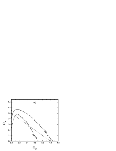
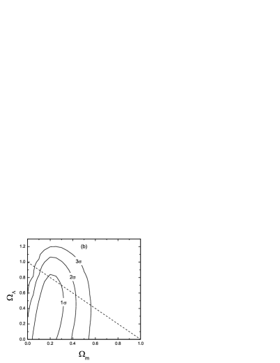
Figure 2: (a) Contour confidence levels of $\Omega_{m}$ and $\Omega_{\Lambda}$ from the GRB data, using method I. (b) Same as panel (a), except now using method II.

With the best-fit flat $\Lambda$CDM model ($\Omega_{m}=0.25$ and $\Omega_{\Lambda}=0.75$), the theoretical distance modulus $\mu_{\rm th}$ is estimated as

$$\mu_{\rm th}(z)\equiv 5\log\left(D_{L}(z)/10\;\rm pc\right)\;.$$ (6)

While, the observed distance modulus $\mu_{\rm obs}$ of each GRB can be calculated using the best-fit Liang-Zhang relation, i.e.,

$$\mu_{\rm obs}=2.5[\kappa_{0}+\kappa_{1}\log E^{\prime}_{\rm p}+\kappa_{2}\log t^{\prime}_{\rm b}-\log(4\pi S_{\gamma}K)+\log(1+z)]-97.45\;.$$ (7)

The Hubble diagram of GRBs then is constructed in Fig. 3, together with the best-fit theoretical line.

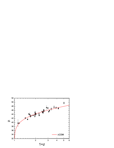
Figure 3: Hubble diagram for 33 GRBs. The solid line shows the theoretical $\mu$.

3 Measuring the High-z Star Formation Rate

The connection of long gamma-ray bursts (LGRBs) with the core collapse of massive stars has been strongly confirmed by many associations between LGRBs and Type Ic supernovae,[74, 75] which may provides a good opportunity for constraining the high-z SFR.[76, 77, 78] Owing to the short lives of massive stars, the SFR can be regarded as their death rate approximatively.

Fig. 4 shows the luminosity-redshift distribution of 244 Swift GRBs, in which the gray shaded region approximates the detection threshold of Swift. For more details on this GRB sample, please see Ref. Wei et al.2014. The luminosity threshold can be estimated using a bolometric flux limit $F_{\rm lim}=1.2\times 10^{-8}$ erg $\rm cm^{-2}$ $\rm s^{-1}$,[48] i.e., $L_{\rm lim}=4\pi D_{L}^{2}F_{\rm lim}$. The Swift/Burst Alert Telescope (BAT) trigger is so complex that it is hard to parametrize exactly the sensitivity of BAT.[79] Furthermore, although the SFR density is well measured at relatively low redshifts ($z\leq 4$), it is poorly constrained at $z\geq 4$. To avoid the complications that would be caused by the use of a detailed treatment of the Swift threshold and the SFR at high-z, we employ a model-independent approach by selecting only bursts with $L_{\rm iso}>L_{\rm lim}$ and $z<4$, as Ref. Kistler et al.2008 did in their treatment. The cut in luminosity is chosen to be equal to the threshold at the maximum redshift of the sample, i.e., $L_{\rm lim}(z=4)\approx 1.8\times 10^{51}$ erg $\rm s^{-1}$. The cut in luminosity and redshift can reduce the selection effects by removing lots of low-$z$, low-$L_{\rm iso}$ bursts that could not be detected at higher redshift. With these conditions, our final tally of GRBs is 118. These data are delimited by the red box in Fig. 4.

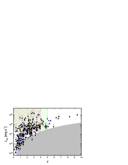
Figure 4: The luminosity-redshift distribution of 244 Swift LGRBs. The blue squares are 13 dark bursts with firm redshift measurements. The gray shaded region represents below the Swift detection threshold. The boxes represent 118 GRBs with $z<4$ and $L_{\rm iso}>1.8\times 10^{51}$ erg $\rm s^{-1}$ (red), and 104 GRBs with $z<5$ and $L_{\rm iso}>3.1\times 10^{51}$ erg $\rm s^{-1}$ (green), respectively.

Since the use of luminosity cuts, the integral of the luminosity function can be treated as a constant coefficient, no matter what the specific form of the luminosity function happens to be. Assuming that the relationship between the comoving GRB rate and the SFR density $\dot{\rho}_{\star}$ can be described as $\dot{n}_{\rm GRB}(z)=\varepsilon(z)\dot{\rho}_{\star}(z)$, where $\varepsilon(z)$ represents the formation efficiency of LGRBs. Now, the expect number of GRBs within a redshift range $(0,\;z)$ can be written as

$$\begin{split}N(<z)\propto\int_{0}^{z}\dot{\rho}_{\star}(z)\frac{\varepsilon(z)}{1+z}\frac{{\rm d}V_{\rm com}}{{\rm d}z}\;{\rm d}z\;,\end{split}$$ (8)

where $\rm d\emph{V}_{com}/d\emph{z}$ is the comoving volume element, and the factor $(1+z)^{-1}$ accounts for the cosmological time dilation. For relatively low redshifts ($z\leq 4$), the SFR density $\dot{\rho}_{\star}$ has been well fitted with a piecewise power law,[62, 80] for which

$$\log\dot{\rho}_{\star}(z)=a+b\log(1+z)\;,$$ (9)

where

$$(a,b)=\left\{\begin{array}[]{ll}(-1.70,3.30),~{}~{}~{}~{}~{}~{}~{}~{}~{}~{}~{}z<0.993\\ (-0.727,0.0549),~{}~{}~{}~{}~{}0.993<z<3.8,\\ \end{array}\right.$$ (10)

and $\dot{\rho}_{\star}$ is in units of $\rm M_{\bigodot}$ $\rm yr^{-1}$ $\rm Mpc^{-3}$.

Fig. 5 shows the cumulative redshift distribution of 118 GRBs (steps), normalized over the redshift range $0<z<4$. In Fig. 5, we compare the observed redshift distribution with three kinds of redshift evolution, characterized through the function $\varepsilon(z)$. If the non-evolution case (i.e., the function $\varepsilon(z)$ is constant) is considered, we find that the expectation from the SFR alone (dotted red line) does not provide a good representation of the observations. If we consider the density evolution model (i.e., $\varepsilon(z)\propto(1+z)^{\alpha}$), we find that the $\chi^{2}$ statistic is minimized for $\alpha=0.8$ and the weak redshift evolution ($\alpha=0.8$) can reproduce the observed redshift distribution quite well (dashed green line). At the $2\sigma$ confidence level, the value of $\alpha$ is in the range $0.07<\alpha<1.53$. It has been proposed that the observationally required evolution may be due to an evolving metallicity.[61, 62] To test this interpretation of the anomalous evolution, we assume that the GRB rate traces the SFR and a cosmic evolution in metallicity, i.e., $\varepsilon(z)\propto\Theta(Z_{\rm th},z)$. Here, $\Theta(Z_{\rm th},z)$ accounts for the fraction of galaxies at redshift $z$ with metallicity below $Z_{\rm th}$,[61] which can be expressed as $\Theta(Z_{\rm th},z)=\hat{\Gamma}\left[\kappa+2,(Z_{\rm th}/Z_{\odot})^{\beta}10^{0.15\beta z}\right]/\Gamma(\kappa+2)$, where $Z_{\odot}$ is the solar metal abundance, $\hat{\Gamma}(a,x)$ and $\Gamma(x)$ are the incomplete and complete Gamma functions, $\kappa=-1.16$ and $\beta=2$.[81, 82] We find that the observations can be well fitted if $Z_{\rm th}=0.52Z_{\odot}$ is adopted (blue line). At the $2\sigma$ confidence level, the value of $Z_{\rm th}$ lies in the range $0.19Z_{\odot}<Z_{\rm th}<0.85Z_{\odot}$. A comparison between this theoretical curve and that obtained with $\varepsilon(z)\propto(1+z)^{0.8}$ shows that the differences between these two fits is very slight. Therefore, we confirm that the anomalous evolution may be due to the cosmic metallicity evolution.

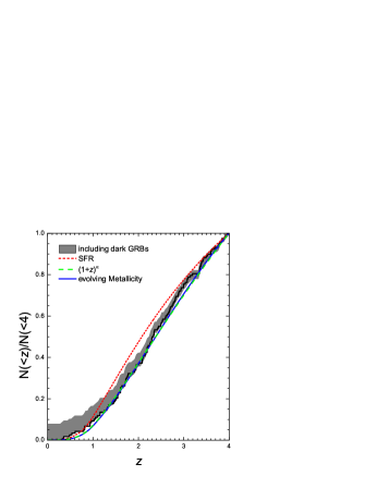
Figure 5: Cumulative redshift distribution of 118 Swift LGRBs with $z<4$ and $L_{\rm iso}>1.8\times 10^{51}$ erg $\rm s^{-1}$ (steps). The red dotted line represents the GRB rate inferred from the SFR. The green dashed line shows the GRB rate inferred from the SFR including $(1+z)^{0.8}$ evolution. The blue solid line corresponds to the GRB rate inferred from the SFR including an evolving metallicity.

In the following, we will consider the implications of these findings for the high-$z$ SFR, assuming that GRBs follow the star formation history and an additional evolution characterized by $(1+z)^{\alpha}$. We will use the best fitting value $\alpha=0.8$ for a reasonable description of this evolutionary effect.

The SFR is now well measured from $z=0$ to 4, but it is not well limited at high-z ($z\geq 4$). In our analysis, a free parameter $\delta$ will be introduced to parametrize the high-z history as a power law at redshifts $z\geq 3.8$:

$$\dot{\rho}_{\star}(z)=0.20\left(\frac{1+z}{4.8}\right)^{\delta},$$ (11)

and this index $\delta$ will be constrained by the GRB observations. The normalization constant in Equation (11) is set by the requirement that $\dot{\rho}_{\star}$ be continuous across $z=3.8$. We optimize the index $\delta$ of high-z SFR by minimizing the $\chi^{2}$ statistic jointly fitting the observed redshift distribution and luminosity distribution of GRBs in our sample. In the density evolution model, the best-fit is produced with a high-z SFR with index $\delta=-3.06_{-2.01}^{+2.01}(1\sigma)$. The range of high-z star formation history with $\delta\in(-5.07,-1.05)$ is marked with an orange shaded band in Fig. 6, in comparison with other observationally determined SFR data.[62, 76, 77, 80, 83, 84, 85]

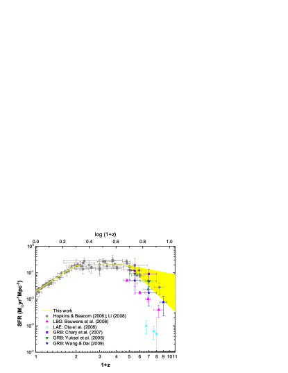
Figure 6: The cosmic star formation history. The high-z SFR (orange shaded region) is constrained by the Swift GRB data, and is characterized by a power-law index $-5.07<\delta<-1.05$. Some available SFR data are also shown for comparison.

Meanwhile, GRBs have indeed already been used to measure the high-$z$ SFR in several works. For example, with deep observations of three $z\sim 5$ GRBs from the Spitzer Space Telescope, a lower limit to the SFR at $z=4.5$ and $6$ was presented in Ref. Chary et al.2007. Ref. Yuksel et al.2008 subsequently made a new determination of the SFR at $z=4-7$ using the $Swift$ GRB data and found that no steep drop exists in the SFR up to $z\sim 6.5$. The use of four years of Swift GRB observations as cosmological probes for the early Universe was discussed by Ref. Kistler et al.2009, who confirmed that the implied SFR to $z\geq 8$ was consistent with Lyman Break Galaxy-based measurements. Ref. Wang et al.2009 used a sample of 119 GRBs to constrain the high-z SFR up to $z\sim 8.3$, showing that the SFR at $z>4$ has a steep decay with a slope of $\sim-5.0$. Based on the principal component analysis method, Ref. Ishida et al.2011 probed cosmic star formation history up to $z\approx 9.4$ from the GRB data and suggested that the level of star formation activity at $z\approx 9.4$ could have been already as high as the present-day one ($\approx 0.01$ $M_{\bigodot}$ $\rm yr^{-1}$ $\rm Mpc^{-3}$).

4 Probing Star Formation in Dark Matter Halos

There is a general agreement about the fact that the rate of LGRBs does not strictly trace the SFR but is actually enhanced by some unknown mechanisms at high-z. Many possible interpretations of the high-z GRB rate excess have been introduced, such as the GRB rate density evolution,[48, 49] the cosmic metallicity evolution,[61, 62] an evolving stellar initial mass function,[63, 64] and an evolution in the break of luminosity function[55, 58, 65, 66]

Nevertheless, it should be underlined that the exception on the LGRB rate relates strongly to the SFR models we adopted. With different star formation history models, the results on the difference between the LGRB rate and the SFR could change on some level.[55, 87] Several forms of SFR are available in the literature. Most of previous works[48, 49, 62, 50, 58, 57] were focused on the the widely accepted SFR model of Ref. Hopkins et al.2006, which provides a good piecewise-linear fit to the numerous multiband observations. However, it is obviously that this empirical fit will vary depending on the observational data and the functional form used. Ref. Hao et al.2013 confirmed that the LGRB rate was still biased tracer of this empirical SFR model. On the contrast, using the self-consistent SFR model calculated from the hierarchical structure formation scenario, they found that a significant fraction of LGRBs occur in dark matter halos with mass down to $10^{8.5}M_{\odot}$ could give an alternative explanation for the discrepancy between the LGRB rate and the SFR.

The fact that stars can form only in structures that are suitably dense, which can be defined by the minimum mass $M_{\rm min}$ of a dark matter halo of the star-forming structures. Thus, no stars will be generated in dark matter halos smaller than $M_{\rm min}$. The minimum halo mass $M_{\rm min}$ must play a crucial role in star formation. The collapsar model suggests that LGRBs are a new promising tool for probing star formation in dark matter halos. In principle, the expected redshift distributions of LGRBs can be calculated from the self-consistent CSFR model as a function of $M_{\rm min}$. Therefore, the minimum halo mass $M_{\rm min}$ can be well constrained by comparing the observed and expected redshift distributions.

Here, we adopt the self-consistent SFR model of Ref. Pereira et al.2010. In the framework of hierarchical structure formation, Ref. Pereira et al.2010 obtained the CSFR by solving the evolution equation of the total gas density that includes the baryon accretion rate, the gas ejection by stars, and the formation of stars through the transfer of baryons in the dark matter halos. In Fig. 7, we show the SFR derived from the self-consistent models with different values of the minimum halo mass $M_{\rm min}$. The observational SFR data taken from Refs. Li2008,Hopkins2004,Hopkins2007. are also shown for comparison. As can be seen, the SFR $\dot{\rho}_{\star}(z)$ is very sensitive to the numerical value of $M_{\rm min}$, especially at high-z. One can also see from this plot that all of these models are in good agreement with observational data at $z\leq 6$.

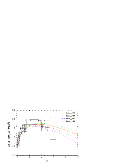
Figure 7: The cosmic SFR as a function of redshift. The curves correspond to the self-consistent models with a minimum halo mass $M_{\rm min}=10^{7.5}$ $\rm M_{\odot}$, $10^{8.0}$ $\rm M_{\odot}$, $10^{8.5}$ $\rm M_{\odot}$, and $10^{9.0}$ $\rm M_{\odot}$, respectively. The observational data are taken from Refs. 89,90 (dots) and Ref. 62 (circles).

In order to compare the observed redshift distribution of LGRBs, we calculate the expected redshift distribution as

$$\frac{\rm d\emph{N}}{\rm d\emph{z}}=F(z)\frac{\varepsilon(z)\dot{\rho}_{\star}(z)}{\langle f_{\rm beam}\rangle}\frac{\rm d\emph{V}_{com}/d\emph{z}}{1+z}\;,$$ (12)

where $\langle f_{\rm beam}\rangle$ denotes the beaming factor and $F(z)$ accounts for the ability both to trigger the burst and to obtain the redshift. Ref. Kistler et al.2008 pointed out that $F(z)$ can be treated as a constant coefficient ($F_{0}$) when we just consider the bright GRBs with luminosities enough to be detected within an entire redshift range. As discussed above, the physical nature of the observed enhancement in the LGRB rate remains under debate. For simplicity, we parametrize the redshift evolution in the LGRB rate as $\varepsilon(z)=\varepsilon_{0}(1+z)^{\alpha}$, where $\varepsilon_{0}$ represents a constant that takes into account the fraction of stars that produce LGRBs. Since the evolutionary index $\alpha$ is conservatively kept as a free parameter, we have two free parameters $M_{\rm min}$ and $\alpha$ in our calculation.

The theoretically expected number of LGRBs within a redshift bin $z_{1}\leq z\leq z_{2}$, for each combination $\textbf{P}\equiv\{M_{\rm min},\alpha\}$, can be expressed as

$$\begin{split}N(z_{1},z_{2};\textbf{P})=\Delta t\frac{\Delta\Omega}{4\pi}\int^{z_{2}}_{z_{1}}F(z)\varepsilon(z)\frac{\dot{\rho}_{\star}(z;M_{\rm min})}{\langle f_{\rm beam}\rangle}\frac{\rm d\emph{V}_{com}/d\emph{z}}{1+z}\;\rm d\emph{z}\\ =\mathcal{A}\int^{\emph{z}_{2}}_{\emph{z}_{1}}(1+\emph{z})^{\alpha}\dot{\rho}_{\star}(\emph{z};M_{\rm min})\frac{\rm d\emph{V}_{com}/d\emph{z}}{1+\emph{z}}\;\rm d\emph{z}\;,\end{split}$$ (13)

where $\mathcal{A}=\Delta t\Delta\Omega F_{0}\varepsilon_{0}/4\pi\langle f_{\rm beam}\rangle$ is a constant that depends on the observed time, $\Delta t$, and the sky coverage, $\Delta\Omega$. The constant $\mathcal{A}$ can be removed by normalizing the cumulative redshift distribution of GRBs to $N(0,z_{\rm max})$, as

$$N(<z|z_{\rm max})=\frac{N(0,z)}{N(0,z_{\rm max})}\;.$$ (14)

With the latest $Swift$ GRBs in hand (see Fig. 4), we attempt to constrain the minimum halo mass $M_{\rm min}$. Owing to the influence of the $Swift$ threshold, those low luminosity bursts can not be detected at higher $z$. To reduce the instrumental selection effect, we also only select luminous bursts with $L_{\rm iso}>1.8\times 10^{51}$ erg $\rm s^{-1}$ and $z<4$, as Ref. Kistler et al.2008 did in their analysis. This cut in luminosity and redshift leaves us 118 GRBs, which are delimited by the red box in Fig. 4. Using the $\chi^{2}$ statistic, we can obtain confidence limits in the two-dimensional ($M_{\rm min}$, $\alpha$) plane by fitting the cumulative redshift distribution of these 118 GRBs. The $1\sigma-3\sigma$ constraint contours of the probability in the ($M_{\rm min}$, $\alpha$) plane are presented in Fig. 8(a). These contours show that at the $1\sigma$ level, $-0.54<\alpha<0.99$, while $M_{\rm min}$ is poorly constrained; only an upper limit of $10^{10.5}$ $\rm M_{\odot}$ can be set at this confidence level. The cross indicates the best-fit pair $(\log M_{\rm min},\;\alpha)=(7.2,\;-0.15)$.

As shown in Fig. 7, the SFR $\dot{\rho}_{\star}(z)$ is very sensitive to the value of $M_{\rm min}$, especially at high-z. For the purpose of exploring the dependence of our results on a possible bias in the high-z bursts, we also consider the sub-sample with $z<5$ and $L_{\rm iso}>L_{\rm lim}(z=5)\approx 3.1\times 10^{51}$ erg $\rm s^{-1}$ (consisting of 104 GRBs). These data are delimited by the green box in Fig. 4. Compared to the previous sub-sample, this sub-sample has 12 more high-$z$ ($4<z<5$) GRBs. We find that adding 12 high-z GRBs could result in much tighter constraints on $M_{\rm min}$. The contours in Fig. 8(b) show that models with $\log M_{\rm min}<7.7$ and $>11.6$ are ruled out at the $1\sigma$ confidence level, which are in agreement with the results of Ref. Munoz et al.2011. The evolutionary index is limited to be $0.10<\alpha<2.55$ ($1\sigma$). The cross indicates the best-fit pair $(\log M_{\rm min},\;\alpha)=(10.5,\;1.25)$.

In a word, we conclude that only moderate evolution of $(1+z)^{\alpha}$ is consistent with the observed GRB redshift distribution over $0<z<4$ or $0<z<5$ ($\sim 1\sigma$ confidence). Although the results of us and previous works[49] are consistent at the $1\sigma$ level, we infer a weaker redshift dependence (i.e., weaker enhancement of the GRB rate compared to the SFR) with lower values of $M_{\rm min}$. Furthermore, the comparison between Fig. 8(a) and Fig. 8(b) can also be found that the best-fit pairs are very different for the two sub-samples. Because of the increased number of high-z bursts at $4<z<5$, the sub-sample with $L_{\rm iso}>3.1\times 10^{51}$ erg $\rm s^{-1}$ and $z<5$ requires a relatively stronger redshift dependence and a higher value of $M_{\rm min}$. Of course, there is still a lot of uncertainty owing to the small high-z GRB sample effect.

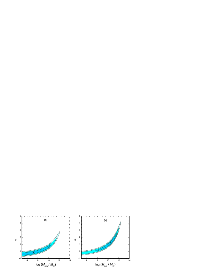
Figure 8: (a): Contour confidence levels of $M_{\rm min}$ and $\alpha$, inferred from the redshift distribution of 118 Swift GRBs with $z<4$ and $L_{\rm iso}>1.8\times 10^{51}$ erg $\rm s^{-1}$. The cross represents the best-fit results. (b): Same as panel (a), except now for 104 Swift GRBs with $z<5$ and $L_{\rm iso}>3.1\times 10^{51}$ erg $\rm s^{-1}$.

5 Conclusions and Discussion

In this paper, we have briefly reviewed the status for the exploration of the early Universe with GRBs. A few solid conclusions and discussion can be summarized:

(i) GRBs can be used as standard candles in constructing the Hubble diagram at high-$z$ beyond the current reach of SNe Ia observations.

However, the dispersion of luminosity relations are still large, which restricted the precision of distance determination with GRBs. Since the classifications of GRBs are not fully understood, some contamination of the GRB sample in a correlation is unavoidable, which would make the correlation be dispersed. Note that among all SNe, only a small class SNe (SNe Ia) can be used as standard candles. On the other hand, the large dispersion may also due to that we have not yet identified the accurate spectral and lightcurve features to use for the luminosity correlations. In order to improve the precision of distance measurement, we should take efforts to investigate the classification problem of GRBs, and search for more precise luminosity relations, especially the relations with certain physical origins.

(ii) GRBs provide an independent and powerful tool to measure the high-$z$ SFR.

The central difficulty of constraining the high-$z$ SFR with GRBs is that one must know the mechanism responsible for the difference between the GRB rate and the SFR. The current Swift GRB observations can in fact be used to explore the unknown mechanism. However, the results from Swift data have uncertainties because of the small GRB sample effect. Fortunately, the upcoming GRB missions such as the Sino-French spacebased multiband astronomical variable objects monitor (SVOM) and the proposed Einstein Probe (EP), with wide field of view and high sensitivity, will be able to discover a sufficiently large number of high-$z$ GRBs. With more abundant observational information in the future, we will have a better understanding of the mechanism for the SFR-GRB rate discrepancy, and we will measure the high-$z$ SFR very accurately using the GRB data alone.

(iii) GRBs also constitute a new promising tool for probing star formation in dark matter halos.

In order to constrain the minimum dark matter halo mass $M_{\rm min}$, we also have to know the relation between the GRB rate and the SFR. In addition to the obvious method of increasing the sample size of GRBs with the help of future dedicated missions, we suggest that a much more severe constraints on $M_{\rm min}$ will be achieved by combining several independent observations, such as the observational data of star formation history, the luminosity distribution of galaxies, and the redshift distribution of GRBs.

References

- [1] Kouveliotou, C., et al., The Astrophysical Journal 413, L101 (1993).
- [2] Woosley, S. E., Bulletin of the American Astronomical Society 25, 894 (1993).
- [3] Woosley, S. E. & J. S. Bloom, Annual Review of Astronomy and Astrophysics 44, 507 (2006).
- [4] Eichler, D., M. Livio, T. Piran, & D. N. Schramm, Nature 340, 126 (1989).
- [5] Narayan, R., B. Paczynski, & T. Piran, The Astrophysical Journal 395, L83 (1992).
- [6] Tanvir, N. R., et al., Nature 461, 1254 (2009).
- [7] Cucchiara, A., et al., The Astrophysical Journal 736, 7 (2011).
- [8] Perlmutter, S., et al., Nature 391, 51 (1998).
- [9] Schmidt, B. P., et al., The Astrophysical Journal 507, 46 (1998).
- [10] Riess, A. G., et al., The Astronomical Journal 116, 1009 (1998).
- [11] Jones, D. O., et al., The Astrophysical Journal 768, 166 (2013).
- [12] Sholl, M. J., et al., Optical, Infrared, and Millimeter Space Telescopes 5487, 1473 (2004).
- [13] Amati, L., et al., Astronomy and Astrophysics 390, 81 (2002).
- [14] Ghirlanda, G., G. Ghisellini, & D. Lazzati, The Astrophysical Journal 616, 331 (2004).
- [15] Yonetoku, D., T. Murakami, T. Nakamura, R. Yamazaki, A. K. Inoue, & K. Ioka, The Astrophysical Journal 609, 935 (2004).
- [16] Liang, E. & B. Zhang, The Astrophysical Journal 633, 611 (2005).
- [17] Schaefer, B. E., The Astrophysical Journal 583, L67 (2003).
- [18] Dai, Z. G., E. W. Liang, & D. Xu, The Astrophysical Journal 612, L101 (2004).
- [19] Ghirlanda, G., G. Ghisellini, D. Lazzati, & C. Firmani, The Astrophysical Journal 613, L13 (2004).
- [20] Schaefer, B. E., The Astrophysical Journal 660, 16 (2007).
- [21] Kodama, Y., D. Yonetoku, T. Murakami, S. Tanabe, R. Tsutsui, & T. Nakamura, Monthly Notices of the Royal Astronomical Society 391, L1 (2008).
- [22] Tsutsui, R., et al., Monthly Notices of the Royal Astronomical Society 394, L31 (2009).
- [23] Firmani, C., G. Ghisellini, G. Ghirlanda, & V. Avila-Reese, Monthly Notices of the Royal Astronomical Society 360, L1 (2005).
- [24] Xu, D., Z. G. Dai, & E. W. Liang, The Astrophysical Journal 633, 603 (2005).
- [25] Amati, L., Monthly Notices of the Royal Astronomical Society 372, 233 (2006).
- [26] Amati, L., et al., Monthly Notices of the Royal Astronomical Society 391, 577 (2008).
- [27] Liang, E. & B. Zhang, Monthly Notices of the Royal Astronomical Society 369, L37 (2006).
- [28] Wang, F. Y. & Z. G. Dai, Monthly Notices of the Royal Astronomical Society 368, 371 (2006).
- [29] Liang, N., W. K. Xiao, Y. Liu, & S. N. Zhang, The Astrophysical Journal 685, 354 (2008).
- [30] Qi, S., F.-Y. Wang, & T. Lu, Astronomy and Astrophysics 487, 853 (2008).
- [31] Qi, S., F.-Y. Wang, & T. Lu, Astronomy and Astrophysics 483, 49 (2008).
- [32] Wei, H. & S.-N. Zhang, European Physical Journal C 63, 139 (2009).
- [33] Yu, B., S. Qi, & T. Lu, The Astrophysical Journal 705, L15 (2009).
- [34] Wei, H., Journal of Cosmology and Astro-Particle Physics 8, 020 (2010).
- [35] Wang, F.-Y., S. Qi, & Z.-G. Dai, Monthly Notices of the Royal Astronomical Society 415, 3423 (2011).
- [36] Wei, J.-J., X.-F. Wu, & F. Melia, The Astrophysical Journal 772, 43 (2013).
- [37] Ding, X., Z. Li, & Z.-H. Zhu, International Journal of Modern Physics D 24, 1550057 (2015).
- [38] Lin, H.-N., X. Li, S. Wang, & Z. Chang, Monthly Notices of the Royal Astronomical Society 453, 128 (2015).
- [39] Izzo, L., M. Muccino, E. Zaninoni, L. Amati, & M. Della Valle, Astronomy and Astrophysics 582, A115 (2015).
- [40] Wei, J.-J., Q.-B. Ma, & X.-F. Wu, Advances in Astronomy 2015, 576093 (2015).
- [41] Ghirlanda, G., G. Ghisellini, C. Firmani, L. Nava, F. Tavecchio, & D. Lazzati, Astronomy and Astrophysics 452, 839 (2006).
- [42] Amati, L. & M. Della Valle, International Journal of Modern Physics D 22, 1330028 (2013).
- [43] Wang, F. Y., Z. G. Dai, & E. W. Liang, New Astronomy Reviews 67, 1 (2015).
- [44] Daigne, F., E. M. Rossi, & R. Mochkovitch, Monthly Notices of the Royal Astronomical Society 372, 1034 (2006).
- [45] Guetta, D. & T. Piran, Journal of Cosmology and Astro-Particle Physics 7, 003 (2007).
- [46] Le, T. & C. D. Dermer, The Astrophysical Journal 661, 394 (2007).
- [47] Salvaterra, R. & G. Chincarini, The Astrophysical Journal 656, L49 (2007).
- [48] Kistler, M. D., H. Yüksel, J. F. Beacom, & K. Z. Stanek, The Astrophysical Journal 673, L119 (2008).
- [49] Kistler, M. D., H. Yüksel, J. F. Beacom, A. M. Hopkins, & J. S. B. Wyithe, The Astrophysical Journal 705, L104 (2009).
- [50] Salvaterra, R., C. Guidorzi, S. Campana, G. Chincarini, & G. Tagliaferri, Monthly Notices of the Royal Astronomical Society 396, 299 (2009).
- [51] Campisi, M. A., L.-X. Li, & P. Jakobsson, Monthly Notices of the Royal Astronomical Society 407, 1972 (2010).
- [52] Qin, S.-F., E.-W. Liang, R.-J. Lu, J.-Y. Wei, & S.-N. Zhang, Monthly Notices of the Royal Astronomical Society 406, 558 (2010).
- [53] Wanderman, D. & T. Piran, Monthly Notices of the Royal Astronomical Society 406, 1944 (2010).
- [54] Cao, X.-F., Y.-W. Yu, K. S. Cheng, & X.-P. Zheng, Monthly Notices of the Royal Astronomical Society 416, 2174 (2011).
- [55] Virgili, F. J., B. Zhang, K. Nagamine, & J.-H. Choi, Monthly Notices of the Royal Astronomical Society 417, 3025 (2011).
- [56] Lu, R.-J., J.-J. Wei, S.-F. Qin, & E.-W. Liang, The Astrophysical Journal 745, 168 (2012).
- [57] Robertson, B. E. & R. S. Ellis, The Astrophysical Journal 744, 95 (2012).
- [58] Salvaterra, R., et al., The Astrophysical Journal 749, 68 (2012).
- [59] Wang, F. Y., Astronomy and Astrophysics 556, A90 (2013).
- [60] Wei, J.-J., X.-F. Wu, F. Melia, D.-M. Wei, & L.-L. Feng, Monthly Notices of the Royal Astronomical Society 439, 3329 (2014).
- [61] Langer, N. & C. A. Norman, The Astrophysical Journal 638, L63 (2006).
- [62] Li, L.-X., Monthly Notices of the Royal Astronomical Society 388, 1487 (2008).
- [63] Xu, C.-y. & D.-m. Wei, Chinese Astronomy and Astrophysics 33, 151 (2009).
- [64] Wang, F. Y. & Z. G. Dai, The Astrophysical Journal 727, L34 (2011).
- [65] Tan, W.-W., X.-F. Cao, & Y.-W. Yu, The Astrophysical Journal 772, L8 (2013).
- [66] Tan, W.-W. & F. Y. Wang, Monthly Notices of the Royal Astronomical Society 454, 1785 (2015).
- [67] Daigne, F., K. A. Olive, J. Silk, F. Stoehr, & E. Vangioni, The Astrophysical Journal 647, 773 (2006).
- [68] Bouché, N., et al., The Astrophysical Journal 718, 1001 (2010).
- [69] Muñoz, J. A. & A. Loeb, The Astrophysical Journal 729, 99 (2011).
- [70] Wei, J.-J., J.-M. Hao, X.-F. Wu, & Y.-F. Yuan, JHEAp 9, 1 (2016).
- [71] D’Agostini, G., ArXiv Physics e-prints arXiv:physics/0511182 (2005).
- [72] Bennett, C. L., et al., The Astrophysical Journal Supplement Series 208, 20 (2013).
- [73] Ghirlanda, G., American Institute of Physics Conference Series 1111, 579 (2009).
- [74] Hjorth, J., et al., The Astrophysical Journal 597, 699 (2003).
- [75] Stanek, K. Z., et al., The Astrophysical Journal 591, L17 (2003).
- [76] Chary, R., E. Berger, & L. Cowie, The Astrophysical Journal 671, 272 (2007).
- [77] Yüksel, H., M. D. Kistler, J. F. Beacom, & A. M. Hopkins, The Astrophysical Journal 683, L5 (2008).
- [78] Trenti, M., R. Perna, E. M. Levesque, J. M. Shull, & J. T. Stocke, The Astrophysical Journal 749, L38 (2012).
- [79] Band, D. L., The Astrophysical Journal 644, 378 (2006).
- [80] Hopkins, A. M. & J. F. Beacom, The Astrophysical Journal 651, 142 (2006).
- [81] Panter, B., A. F. Heavens, & R. Jimenez, Monthly Notices of the Royal Astronomical Society 355, 764 (2004).
- [82] Savaglio, S., New Journal of Physics 8, 195 (2006).
- [83] Bouwens, R. J., G. D. Illingworth, M. Franx, & H. Ford, The Astrophysical Journal 686, 230 (2008).
- [84] Ota, K., et al., The Astrophysical Journal 677, 12 (2008).
- [85] Wang, F. Y. & Z. G. Dai, Monthly Notices of the Royal Astronomical Society 400, L10 (2009).
- [86] Ishida, E. E. O., R. S. de Souza, & A. Ferrara, Monthly Notices of the Royal Astronomical Society 418, 500 (2011).
- [87] Hao, J.-M. & Y.-F. Yuan, The Astrophysical Journal 772, 42 (2013).
- [88] Pereira, E. S. & O. D. Miranda, Monthly Notices of the Royal Astronomical Society 401, 1924 (2010).
- [89] Hopkins, A. M., The Astrophysical Journal 615, 209 (2004).
- [90] Hopkins, A. M., The Astrophysical Journal 654, 1175 (2007).