The Cassie-Wenzel transition of fluids on nanostructured substrates: Macroscopic force balance versus microscopic density-functional theory

Abstract

Classical density functional theory is applied to investigate the validity of a phenomenological force-balance description of the stability of the Cassie state of liquids on substrates with nanoscale corrugation. A bulk free-energy functional of third order in local density is combined with a square-gradient term, describing the liquid-vapor interface. The bulk free energy is parameterized to reproduce the liquid density and the compressibility of water. The square-gradient term is adjusted to model the width of the water-vapor interface. The substrate is modeled by an external potential, based upon Lennard-Jones interactions. The three-dimensional calculation focuses on substrates patterned with nanostripes and square-shaped nanopillars. Using both the force-balance relation and density-functional theory, we locate the Cassie-to-Wenzel transition as a function of the corrugation parameters. We demonstrate that the force-balance relation gives a qualitatively reasonable description of the transition even on the nanoscale. The force balance utilizes an effective contact angle between the fluid and the vertical wall of the corrugation to parameterize the impalement pressure. This effective angle is found to have values smaller than the Young contact angle. This observation corresponds to an impalement pressure that is smaller than the value predicted by macroscopic theory. Therefore, this effective angle embodies effects specific to nanoscopically corrugated surfaces, including the finite range of the liquid-solid potential (which has both repulsive and attractive parts), line tension, and the finite interface thickness. Consistently with this picture, both patterns (stripes and pillars) yield the same effective contact angles for large periods of corrugation.

I Introduction

Super liquid-repellent surfaces are important for fundamental studies of wetting phenomena, as well as technological applications, including anti-fouling coatings Yao, Song, and Jiang (2011), fog harvesting Park et al. (2013), drag reduction Watanabe and Udagawa (2001); Gogte et al. (2005); Drappier et al. (2006); Ou, Perot, and Rothstein (2004), and gas exchange membranes McHale, Newton, and Shirtcliffe (2010); Paven et al. (2013). Micro- and nanoscale topographic structuring offers significant opportunities for manufacturing such surfaces, by introducing a special wetting mode – the Cassie or the “fakir” state Cassie and Baxter (1944). In this regime, the liquid resides on top of the topographic corrugations, while the enclosed space below the liquid is filled with gas (Fig. 1a). This reduces the adhesion, and a droplet can roll off easily. Thermodynamically, however, the Cassie state is frequently only metastable Bormashenko (2015); Callies and Quéré (2005); Dorrer and Rühe (2009); Nosonovsky and Bhushan (2007), meaning that it corresponds to only a local minimum of the free energy, compared to the free energy of a slightly deformed droplet. In such a metastable situation, the absolute free-energy minimum rather corresponds to the complete-wetting or Wenzel state Wenzel (1936). In the Wenzel state, the liquid permeates the topographic structure, such that no gas “pockets” remain, the adhesion is increased, and the contact angle exhibits a large hysteresis (Fig. 1b). The Wenzel state is therefore usually not super-repellent Callies and Quéré (2005), and hence most technological applications aim at avoiding it as much as possible.

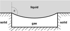
(a)

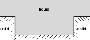
(b)

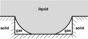
(c)

Figure 1: Various wetting regimes in the simplified two-dimensional geometry: (a) Cassie state, where the liquid-gas interface resides on top of the solid corrugations; (b) Wenzel state, where the liquid permeates the cavity between the topographic structure, and (c) Sagging mechanism in the Cassie state, where the liquid-gas interface still resides on top of the corrugations but due to its curvature (or corrugation dimensions) gets into contact with the bottom of the cavity.

To understand the basic physics of the system, let us consider the coexistence of the liquid and the gas phase, in the presence of the surface. Let us also assume, as a first step, that the surface is flat. Since it is repelling, it is clear that an open system at a pressure slightly above the bulk coexistence pressure will be “dry”. In other words, the condensed liquid phase exists away from the surface, while direct contact with it is avoided. However, the “dry” layer is very thin; its thickness is roughly comparable to the range of interaction of the repulsion. From a macroscopic point of view, this means contact, but with a large interfacial tension $\gamma_{\rm sl}$ between solid and liquid. Now we add a groove to the surface, and we first assume that it is infinitely deep. In this situation, the system can either be in the Cassie state, where the liquid-gas interface remains suspended above the groove, or in the Wenzel state, where the whole groove is filled with liquid. This is so because pushing the interface into the groove by a length $h$ results in a gain of bulk free energy that scales linearly with $h$, but also in a loss of liquid-solid surface free energy that scales linearly with $h$ as well. Since the system prefers a liquid-gas interface over a liquid-solid interface, the Cassie state is preferred, unless the bulk pressure is so large that the bulk free energy prevails and the system chooses the Wenzel state. For a groove that is an infinitely long stripe, this consideration results in a critical excess pressure (additional pressure above the gas value) of

$$P^{\rm max}=-\frac{2\gamma}{D}\cos\Theta_{\textrm{flat}},$$ (1)

where $D$ is the width of the groove, $\gamma$ the liquid-gas interface tension, and $\Theta_{\textrm{flat}}$ the Young contact angle of a macroscopic liquid droplet on a flat surface (larger than $90^{\circ}$, due to the repelling surface). For a derivaton of this relation Bormashenko (2015); Dorrer and Rühe (2009); Extrand (2002); Zheng, Yu, and Zhao (2005); Bartolo et al. (2006); Cottin-Bizonne et al. (2004); Moulinet and Bartolo (2007); Butt, Vollmer, and Papadopoulos (2014), see Appendix A. Within this picture, the Cassie-Wenzel transition may therefore be viewed as a first-order phase transition. From the experimental point of view, it is useful to re-write the relation as

$$P^{\rm max}=-\frac{L_{\rm c}}{A}\frac{\gamma\cos\Theta_{\rm max}}{1-f},$$ (2)

where we assume that the total surface has an area $A$, of which a fraction $f$ is wetted in the Cassie state, while the fraction $1-f$ is covered with gas. More precisely, we mean by $A$ the area that is obtained after projecting the nanostructure onto the surface, and similarly for the fractions $Af$ and $A(1-f)$. Furthermore, $L_{\rm c}$ denotes the contour length of the contact line, while $\Theta_{\rm max}$ replaces $\Theta_{\textrm{flat}}$ as the maximum contact angle; this is an effective angle that takes into account that the grooves in general have a different shape than one-dimensional stripes Moulinet and Bartolo (2007). It should also be noted that the physical origin of the pressure is of course arbitrary Bartolo et al. (2006); e. g. it can be the Laplace pressure due to the curvature of the deposited droplet, a dynamic pressure during droplet impact on the surface, or hydrostatic pressure (underwater superhydrophobicity Hemeda and Tafreshi (2014)).

This simple phenomenological picture has been experimentally confirmed, e. g., in the observation of evaporating droplets Moulinet and Bartolo (2007). Here the Laplace pressure de Gennes, Brochard-Wyart, and Quéré (2004) keeps on increasing during the evaporation process, until it reaches $P^{\rm max}$ (and the contact angle $\Theta_{\rm max}$), and the Cassie state collapses.

However, in general we may have to take into account that the groove has a finite depth. In this situation, the Cassie and Wenzel states look like depicted in Figs. 1a and 1b, respectively. Apart from these two cases, it is then in principle possible that yet a third stable state occurs. It is depicted in Fig. 1c and we refer to it as the “sagged Cassie” (SC) state. Here the contact line at the “upper” end of the groove still remains pinned, but the liquid-gas interface is already in contact with the “bottom” of the cavity, while gas pockets remain in the corners of the groove. Such a state typically requires strong hydrophobicity, in order to make sure that the contact angle at the onset of sagging is still below the Young angle. Another possibility to reach the SC state consists of very shallow grooves, with a small depth-to-width ratio. However, for these latter systems the involved pressures are quite small, which means that they are very difficult to control and handle. For these reasons, the SC state has so far rarely been of experimental importance. Conversely, within the framework of theoretical calculations as described below, it is, for large hydrophobicity, quite easily possible to observe the SC state. As a matter of fact, we did observe it for a system with a Young contact angle of roughly $150^{\circ}$. However, the purpose of the present paper is mainly a test of the theory of the Cassie-Wenzel transition (i. e. essentially Eq. (2)), which obviously does not apply to the SC state. For this reason, we have deferred a study of these phenomena to future work, and confined the present investigation to systems where a direct Cassie-Wenzel transition occurs.

Equation (2) shows clearly the challenges of manufacturing good super-repellent surfaces. Firstly, one should realize that the ratio $L_{\rm c}/A$ is $\sim l^{-1}$, where $l$ is the characteristic length scale of the corrugation geometry, assuming that its basic structure type (stripes, pillars, etc.) remains fixed. Now, one would like to make $f$ as small as possible in order to facilitate easy roll-off Callies and Quéré (2005). However, to stabilize the Cassie state (or to increase $P^{\rm max}$) one would like to make $f$ as large as possible. In principle, this problem is avoided if $l$ is decreased at constant $f$, meaning that both the period of the corrugation and the lateral dimensions of the asperities are decreased at the same rate: In this case, $P^{\rm max}$ increases without sacrificing the frictional properties. However, this “miniaturization route” Extrand (2006); Zheng, Yu, and Zhao (2005); Moulinet and Bartolo (2007); Bormashenko (2015); Butt, Vollmer, and Papadopoulos (2014) is of course experimentally difficult.

It is thus obvious that it is highly interesting to understand the Cassie-Wenzel transition for nanoscopically structured surfaces. Here, however, one should take into account that Eq. (2) is based upon a macroscopic consideration. At the nanoscale, there are many aspects beyond macroscopic physics, which potentially can alter the picture – or at least modify it when it comes to quantitative considerations. Such aspects are (i) the finite thickness of the liquid-gas interface, (ii) line tension effects, (iii) the finite range of the substrate potential, (iv) the atomic structure of the substrate, (v) the atomic structure of the liquid, and (vi) thermal fluctuations. It is thus not quite clear to what extent Eq. (2) remains valid at the nanoscale Butt, Vollmer, and Papadopoulos (2014). Recent in situ x-ray diffraction studies Checco et al. (2014) of the Cassie-Wenzel transition indicate that this might be indeed the case. However, to the best of our knowledge, extensive theoretical studies of this question are still lacking, and the present paper is intended as a step in this direction. We therefore investigate a simple microscopic model and compare its predictions for the stability of the Cassie state with Eq. (2). In the present study only the microscopic aspects (i)–(iii) are taken into account, such that the calculations are not too compute-intensive, and a large range of parameters can be explored. It is possible to refine the model and include the aspects (iv)–(vi); this is however left for future work.

Similar theoretical studies exist, which investigate microscopic models at structured surfaces. However, these focus mainly on the dynamics, which is of course also highly interesting and important. Apart from analytical theories Marmur (2004); Patankar (2004) there is currently significant interest in exploring the barriers and the transition pathways between the two states. This can be done by lattice Boltzmann simulations Dupuis and Yeomans (2005); Gross et al. (2010), string-method calculations cast in the framework of continuum descriptions Ren (2014) and particle-based Molecular Dynamics (MD) Giacomello et al. (2015), as well as Boxed MD Savoy and Escobedo (2012).

In the current study, we employ an approach based on the classical density functional theory (DFT) for liquids. Due to the flexibility of the formalism, wetting phenomena can be addressed within DFT at different levels of detail, as has been extensively discussed in several reviews Evans (1979); Dietrich (1988); Tarazona, Marconi, and Evans (1987); Wu (2006); Weeks, Vollmayr, and Katsov (1997). A simple strategy, which we employ here, is to consider functionals which neglect the molecular structure of the liquid and therefore do not account for, e. g., layering at walls. At this level, the interactions between liquid molecules (i. e. the fact that below the liquid-gas transition the molecules tend to aggregate) is just taken into account by the square-gradient approximation Cahn and Hilliard (1958), while the bulk thermodynamics is described by a strictly local functional.

More sophisticated functionals, like, e. g., the weighted density approximation Tarazona (1985), or even more elaborate schemes Lum, Chandler, and Weeks (1999); Hughes, Krebs, and Roundy (2013); Yang et al. (1992); Yang, Sullivan, and Gray (1994); Clark et al. (2006); Lischner and Arias (2010); Sundararaman, Letchworth-Weaver, and Arias (2012), can be constructed, such that details of short-range correlations in the liquid are faithfully modeled. However, these elaborate functionals are computationally much more expensive, and hence have not been used in the present exploratory study. Representative studies of liquids on chemically or topographically patterned substrates (but only in two dimensions!), based upon such functionals, can be found in Refs. Koch, Dietrich, and Napiórkowski (1995); Malijevský (2014); Berim and Ruckenstein (2015), while our simple functional allows us to study three-dimensional systems without major problems. This DFT model is parameterized on the basis of a few thermodynamic properties of water, known from experiments. The liquid-substrate interactions are taken into account by a Lennard-Jones potential. Several cases of strength of water/solid interactions are considered, realizing different degrees of hydrophobicity of the surface. A highly related previous DFT study by Zhang and Ren Zhang and Ren (2014) was done in three dimensions as well, and resulted in Cassie-Wenzel phase diagrams for various surface patterns. In contrast to the present study, whose aim is the comparison with macroscopic theory, Ref. Zhang and Ren, 2014 rather focused on transition states investigated with the “string method” and did not attempt to adjust the functional to an experimental system. Our study should therefore be viewed as complementary to Ref. Zhang and Ren, 2014.

The paper is organized as follows: Sec. II presents the modeling strategy. In particular, the classical DFT approach is introduced in Sec. II.1, while Sec. II.2 explains the parameterization. The method of incorporating corrugated substrates into the model is discussed in Sec. II.3 and the numerical scheme is elaborated in Sec. II.4. We proceed with contact angle calculations in the canonical ensemble in Sec. III.1. The predictions of the phenomenological force balance and the classical DFT calculations on nanostructured substrates are compared in the remainder of Sec. III. We conclude in Sec. IV with a short summary and an outlook.

II Modeling approach

II.1 Density functional theory description

We study the equilibrium thermodynamics of a system with volume $V$ and temperature $T$ in the grand-canonical ensemble. The starting point is a grand-canonical potential $\Omega$, which is a functional of the average local number density $\rho({\bf r})$:

$$\Omega = \int d{{\bf r}}\;\omega(\rho(\mathbf{r}),\nabla\rho(\mathbf{r})),$$ (3)

$$\frac{\omega}{k_{B}T} = \rho({\bf r})\left[\ln(\Lambda^{3}\rho({\bf r}))-1\right]+f_{\rm b}(\rho({\bf r}))+$$ (4)

$$\frac{\kappa}{2}\left(\nabla\rho({\bf r})\right)^{2}+U_{\textrm{s}}({\bf r})\rho({\bf r})-\mu\rho({\bf r}).$$

Here $k_{B}T$ is the thermal energy, such that $\Omega/k_{B}T$ is dimensionless. The first term in Eq. (4) describes the translational entropy of the liquid molecules. $\Lambda$ is usually taken as the thermal de Broglie wavelength, which gives rise to a normalization volume $\Lambda^{3}$ that is needed for dimensional reasons. Actually, the value of $\Lambda$ is immaterial, since it only serves to define the zero of the dimensionless chemical potential $\mu$ in the last term. This is seen from the trivial identity

$$\rho\ln(\Lambda^{3}\rho)-\mu\rho=\rho\ln\left(\frac{\rho}{\Lambda^{-3}\exp(\mu)}\right),$$ (5)

which means that the only relevant parameter is the combination $\Lambda^{-3}\exp(\mu)$. The bulk excess Helmholtz free energy per unit volume and per $k_{B}T$ is denoted by $f_{\rm b}(\rho({\bf r}))$. The square-gradient term penalizes the presence of liquid-gas interfaces Cahn and Hilliard (1958). $\kappa$ controls the interfacial width and, in general, can be density-dependent Yang, Fleming, and Gibbs (1976); Anderson, McFadden, and Wheeler (1998). In the present study, $\kappa$ is assumed to be a constant. The influence of the substrate is described by an external potential (per $k_{B}T$) denoted by $U_{\rm s}({\bf r})$. The form of this potential, specific to the current study, is discussed in sec. II.3. It should be noted that $U_{\rm s}$ is dimensionless, while $f_{\rm b}$ has the dimension of an inverse volume. For $f_{\rm b}(\rho({\bf r}))$ we choose

$$f_{\rm b}(\rho({\bf r}))=\frac{v}{2}\rho({\bf r})^{2}+\frac{w}{3}\rho({\bf r})^{3}$$ (6)

with constant coefficients $v$ and $w$. This is a very simple model capable of describing liquid-gas coexistence, due to the competition between attraction ($v<0$) and repulsion ($w>0$). These coefficients, and also the interface parameter $\kappa$, are chosen to reproduce some reference properties of liquid water (see Sec. II.2 for details).

The equilibrium density distribution minimizes $\Omega$ and therefore fulfills the corresponding Euler-Lagrange equation:

$$\ln(\Lambda^{3}\rho({\bf r}))+\frac{\partial f_{\rm b}(\rho({\bf r}))}{\partial\rho({\bf r})}-\kappa\mathbf{\nabla}^{2}\rho({\bf r})+U_{\textrm{s}}({\bf r})-\mu=0.$$ (7)

To re-cast this DFT description in terms of Self Consistent Field (SCF) theory Thompson (2006); Müller, MacDowell, and Yethiraj (2003); Bryk and MacDowell (2008), it is instructive to rewrite Eq. (7) as a system of equations:

$$W({\bf r}) = \frac{\partial f_{\rm b}(\rho({\bf r}))}{\partial\rho({\bf r})}-\kappa\mathbf{\nabla}^{2}\rho({\bf r})+U_{\textrm{s}}({\bf r}),$$ (8)

$$\rho({\bf r}) = \Lambda^{-3}\exp(\mu)\exp(-W({\bf r})).$$ (9)

The quantity $W({\bf r})$ plays the role of a mean field representing the interactions of a liquid molecule with its surrounding molecules and the substrate. Apart from illustrating the link to the SCF theory framework, Eqs. (8) and (9) also provide the basis for our numerical scheme.

For a bulk liquid with density $\rho_{\rm b}$, the density profile is constant, and the surface potential vanishes. In this situation, Eqs. (8) and (9) are simplified to

$$\Lambda^{-3}\exp(\mu)=\rho_{\rm b}\exp\left(\frac{\partial f_{\rm b}}{\partial\rho}\Big{|}_{\rho=\rho_{\rm b}}\right).$$ (10)

Inserting Eq. (10) into Eq. (9), one sees that instead of the chemical potential we can rather use $\rho_{\rm b}$ in the liquid phase as a control parameter.

For our nanoscopic system with an interface, the concept of pressure needs to be generalized to the concept of a stress tensor $\tensor{\Pi}(\mathbf{r})$. From the general principles of Lagrangian field theory Landau and Lifshitz (1975) it is clear that the stress tensor is calculated as

$$\tensor{\Pi}=\frac{\partial\omega}{\partial\nabla\rho}\otimes\nabla\rho-\omega\;\tensor{1};$$ (11)

for our functional this results in Yang, Fleming, and Gibbs (1976)

$$\frac{\tensor{\Pi}}{k_{B}T} = \kappa\left[\nabla\rho\otimes\nabla\rho-\frac{1}{2}\left(\nabla\rho\right)^{2}\tensor{1}\right]$$

$$-\left[\rho(\ln(\Lambda^{3}\rho)-1)+f_{\rm b}+U_{s}\rho-\mu\rho\right]\tensor{1}.$$

For an infinite homogeneous bulk system, the expression becomes much simpler: $\tensor{\Pi}=P\tensor{1}$ with

$$\frac{P}{k_{B}T}=-\rho_{\rm b}(\ln(\Lambda^{3}\rho_{\rm b})-1)-f_{\rm b}(\rho_{\rm b})+\mu\rho_{\rm b}.$$ (13)

Again we can use Eq. (10) to eliminate the chemical potential; this results in the equation of state

$$\frac{P}{k_{B}T}=\rho_{\rm b}+\rho_{\rm b}\left.\frac{\partial f_{\rm b}}{\partial\rho}\right|_{\rho=\rho_{\rm b}}-f_{\rm b}(\rho_{\rm b}).$$ (14)

The stress tensor can therefore also be re-written as

$$\frac{\tensor{\Pi}}{k_{B}T} = \kappa\left[\nabla\rho\otimes\nabla\rho-\frac{1}{2}\left(\nabla\rho\right)^{2}\tensor{1}\right]$$ (15)

$$+P_{\rm bulk}\tensor{1}-U_{\rm s}\rho\tensor{1},$$

with the understanding that the abbreviation $P_{\rm bulk}$ means the evaluation of the bulk equation of state for the local density $\rho(\mathbf{r})$.

When adjusting $U_{\textrm{s}}({\bf r})$ to reproduce a desired contact angle on a non-corrugated substrate, the canonical ensemble is more convenient. The Euler-Lagrange equation is then derived by minimizing the Helmholtz free energy, obtained from Eq. (4). This must be done under the constraint that the total number of molecules $N$ in the system remains fixed. In this case, the relationship between the mean field felt by the molecule and the local density is still described by Eq. (8). However the counterpart of Eq. (9) in the canonical ensemble is

$$\rho({\bf r})=\frac{N\exp(-W({\bf r}))}{\int d{{\bf r^{\prime}}}\exp(-W({\bf r^{\prime}}))}.$$ (16)

II.2 Parameterization

At ambient conditions ($T=298.15\,\mathrm{K}$, $P=P_{\rm a}=0.1013\,\mathrm{MPa}$, $P/k_{B}T=0.0246\,(\mathrm{nm})^{-3}$) liquid water has Lide (2004) a density (number of molecules per volume) of $\rho_{\rm a}=33.33\,(\mathrm{nm})^{-3}$, and a bulk modulus $K=\rho\partial P/\partial\rho=2.21\,\mathrm{GPa}$, or $K/k_{B}T=537\,(\mathrm{nm})^{-3}$. From the equation of state, Eq. (14), combined with the simple model free energy, Eq. (6), we find for pressure and modulus

$$\frac{P}{k_{B}T} = \rho+\frac{v}{2}\rho^{2}+\frac{2}{3}w\rho^{3},$$ (17)

$$\frac{K}{k_{B}T} = \rho+v\rho^{2}+2w\rho^{3}.$$ (18)

Insertion of the the values for $\rho$, $P/(k_{B}T)$, and $K/(k_{B}T)$, as given above for ambient conditions, gives rise to a set of two linear equations for $v$ and $w$. Its solutions is $v\approx-1.09\,(\mathrm{nm})^{3}$, and $w\approx 0.023\,(\mathrm{nm})^{6}$. Throughout the study, we consider the temperature $T=298.15\,\mathrm{K}$.

Bulk phase coexistence between liquid and vapor occurs at a significantly lower pressure $P_{\rm c}<P_{\rm a}$. Denoting the densities in the liquid and vapor phases with $\rho_{\rm l}$ and $\rho_{\rm v}$, respectively, the conditions for phase coexistence are (i) equality of the pressure, i. e.

$$\rho_{\rm l}+\frac{v}{2}\rho_{\rm l}^{2}+\frac{2}{3}w\rho_{\rm l}^{3}=\rho_{\rm v}+\frac{v}{2}\rho_{\rm v}^{2}+\frac{2}{3}w\rho_{\rm v}^{3},$$ (19)

and (ii) equality of the chemical potential, i. e.

$$\rho_{\rm l}\exp\left(v\rho_{\rm l}+w\rho_{\rm l}^{2}\right)=\rho_{\rm v}\exp\left(v\rho_{\rm v}+w\rho_{\rm v}^{2}\right)$$ (20)

(cf. Eq. (10)). To determine $\rho_{\rm l}$ and $\rho_{\rm v}$ one needs to solve this set of equations numerically. For the parameters given above, this results in a liquid density that is slightly decreased relative to the ambient value, but essentially the same, due to the large value of $K$ (and identical within the given accuracy). The vapor density is found to be $\rho_{\rm v}\approx 8.7\times 10^{-4}\,(\mathrm{nm})^{-3}$, while the coexistence pressure (in units of $k_{B}T$) is found to be $P_{\rm c}/k_{B}T\approx 8.7\times 10^{-4}\,(\mathrm{nm})^{-3}$, which is equivalent to $P_{\rm c}\approx 3.6\,\mathrm{kPa}$.

Since $K$ is very large, one can alternatively solve the problem with fairly good accuracy in a simpler way, and this is the way how we actually determined our parameters: We assume from the outset that at coexistence the liquid density $\rho_{\rm l}$ takes the value $\rho_{\rm a}$, i. e. we neglect the tiny decrease in density that results from decreasing the pressure from one atmosphere to the coexistence value. We then consider Eqs. (18), (19), and (20) as three equations for the three unknowns $v$, $w$, and $\rho_{\rm v}$, which are solved simultaneously, while the coexistence pressure is determined after this from Eq. (17). This results in $v$, $w$, $\rho_{\rm v}$, and $P_{\rm c}$ values that are slightly shifted but, within the given accuracy, identical to the values already given. The precise values of the parameters at which the study was performed are $v=-1.086641506142464\,(\mathrm{nm})^{3}$ and $w=0.023102120829070\,(\mathrm{nm})^{6}$. The vapor density and the coexistence pressure are reasonably close to their experimental counterparts Lide (2004), $\rho_{\rm v}\approx 7.7\times 10^{-4}\,(\mathrm{nm})^{-3}$ and $P_{\rm c}\approx 3.2\,\mathrm{kPa}$. It should be emphasized that, taking into account the simplicity of the free-energy functional, it can be hardly expected to reproduce real experimental data more faithfully. Nevertheless, the most important properties of bulk water have been taken into account.

To estimate the parameter $\kappa$ we consider a flat liquid-vapor interface in the absence of a substrate potential. The one-dimensional density profile $\rho(z)$ then varies between $\rho_{\rm v}$ for $z\to-\infty$ and $\rho_{\rm l}$ for $z\to+\infty$. The surface tension $\gamma$ is then given by Jones and Richards (1999); Yang, Fleming, and Gibbs (1976)

$$\frac{\gamma}{k_{B}T}=\kappa\int_{-\infty}^{+\infty}dz\left(\frac{d\rho(z)}{dz}\right)^{2}.$$ (21)

To proceed, we note that the problem of finding the one-dimensional density profile $\rho(z)$ is mathematically identical to solving the one-dimensional equation of motion of a particle in an external potential, by identifying $\Omega$ with the action integral. The standard method to solve such a problem Landau and Lifshitz (1976) is to write down the equation for energy conservation and to separate variables. This allows us, after eliminating $\mu$, and some straightforward algebra, to transform the integral to the form

$$\frac{\gamma}{k_{B}T}=\sqrt{\kappa}\int_{\rho_{\rm v}}^{\rho_{\rm l}}d\rho\;\sqrt{2\phi(\rho)}$$ (22)

with

$$\phi(\rho) = \rho\ln\left(\frac{\rho}{\rho_{\rm l}}\right)+\left(\rho_{\rm l}-\rho\right)+\frac{v}{2}\left(\rho_{\rm l}^{2}+\rho^{2}\right)$$ (23)

$$+\frac{w}{3}\left(2\rho_{\rm l}^{3}+\rho^{3}\right)-\rho\left(v\rho_{\rm l}+w\rho_{\rm l}^{2}\right).$$

Numerical evaluation yields

$$\frac{\gamma}{k_{B}T}=\sqrt{\kappa}\cdot 199.26\,\textrm{nm}^{-9/2}.$$ (24)

Experimentally Kayser (1976) $\gamma=0.07275\,\mathrm{N/m}$ or $\gamma/k_{B}T=17.673\,\textrm{nm}^{-2}$ and we thus obtain $\kappa=0.007866\,(\mathrm{nm})^{5}$.

The interfacial width $h$ can be estimated approximately by assuming a profile that is linear on a scale $h$ and flat otherwise. This yields (see Eq. 21)

$$\frac{\gamma}{k_{B}T}\approx\frac{\kappa}{h}(\rho_{\textrm{l}}-\rho_{\textrm{v}})^{2}$$ (25)

or $h\approx 0.5\,\textrm{nm}$. This would however impose the need of a very fine discretization grid. We therefore increase $\kappa$ to the value $\kappa=0.031478342\,(\mathrm{nm})^{5}$ (actual value used in the calculations). This implies $\gamma=0.1455\,\textrm{N/m}$ and $h\approx 1\,\textrm{nm}$ (since $\gamma\propto\sqrt{\kappa}$ it follows from Eq. 25 that $h\propto\sqrt{\kappa}$). This allows us to perform the calculations employing a lattice spacing of $0.1\,\textrm{nm}$, which reduces the computational effort significantly, compared to the otherwise needed value of $0.05\,\textrm{nm}$. Furthermore, according to the simulation results of Ref. Sedlmeier, Horinek, and Netz (2009), an interfacial width of $1\,\textrm{nm}$ is also expected to be physically more realistic.

II.3 Corrugated substrates

We model the corrugation geometry by a function $\rho_{0}(\mathbf{r})$, the number density of the substrate atoms. We assume that this function is constant (i. e. $\rho_{0}(\mathbf{r})=\rho_{0}$) within the space occupied by the substrate and zero elsewhere. Describing the substrate in terms of continuum theory (just as the water), and assuming pairwise additive interactions, we can hence write

$$U_{\rm s}(\mathbf{r})=\int d{\bf r^{\prime}}\;U_{\rm sw}\left(\left|\mathbf{r}-\mathbf{r^{\prime}}\right|\right)\rho_{0}\left(\mathbf{r^{\prime}}\right),$$ (26)

where $U_{\rm sw}$ is the interaction potential between a substrate atom and a water molecule (in units of $k_{B}T$). For the latter, we use a 12-6 Lennard-Jones (LJ) potential:

$$U_{\rm sw}(r)=\left\{\begin{array}[]{l l}\frac{4\epsilon}{k_{B}T}\left[\left(\frac{\sigma}{r}\right)^{12}-\left(\frac{\sigma}{r}\right)^{6}\right]&r\leq r_{\rm c},\\ 0&r>r_{\rm c},\end{array}\right.$$ (27)

where $\epsilon$ and $\sigma$ are the characteristic energy and length scale, respectively. In our calculations we use $\sigma=0.3\,\mathrm{nm}$ and $r_{\textrm{c}}=5\,\mathrm{nm}$, while the potential depth $\epsilon$ is adjusted to reproduce the desired contact angle on a flat substrate. More precisely, it is only the combined parameter $\tilde{\epsilon}=\epsilon\rho_{0}/k_{B}T$ that matters, and this is what we vary.

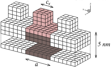
Figure 2: (color online) Set-up for defining the substrate potential. The substrate explicitly present in the calculation box is shown in pink. To construct the substrate potential a ”bulk” of the substrate is taken into account (brown). The obtained substrate unit is subsequently replicated (for clarity only two images in $x$-direction are shown in white) based on the cut-off $r_{\textrm{c}}$ of the LJ potential.

As the substrate structure is strictly periodic in the $x$ and $y$ directions (parallel to the surface), it is sufficient to restrict attention to one unit cell of the corrugation. This results in a simulation cell with periodic boundary conditions in $x$ and $y$ directions. The space $z\leq 0$ corresponds to the “bulk” substrate, i. e. $\rho_{0}(\mathbf{r})=\rho_{0}$ whenever $z<0$. In contrast, the space $z>0$ corresponds to the corrugated part, i. e. here we have $\rho_{0}(\mathbf{r})=0$ for the space left for the water, while $\rho_{0}(\mathbf{r})=\rho_{0}$ in the regions where there is substrate material. In $z$ direction we hence choose a box size that is large enough to faithfully model (i) the interactions with all the substrate atoms, and (ii) the thermal equilibrium with a bulk reservoir of water. This requires an extension of at least $r_{\rm c}$ in the negative $z$ direction, and an extension in positive $z$ direction that is significantly larger than the size of the corrugation, plus the interfacial width. A typical unit cell is illustrated in Fig. 2 in pink (one repeat unit of corrugation) and brown (“bulk” of the substrate).

The continuum theory is discretized in terms of a simple cubic grid with lattice spacing $\Delta L=0.1\,\mathrm{nm}$, and for simplicity we choose the same lattice structure and constant in both the space occupied by water and substrate. The integral in Eq. (26) is then discretized by a sum, which has to be evaluated once and for all at the beginning of the calculation (i. e. with negligible computational cost). This formula is however used only for those sites $\mathbf{r}$ that are not occupied by the substrate.

In order to avoid complicated boundary conditions at the substrate surface, we allow (in principle) the water to penetrate into the substrate. In other words, the equations are solved everywhere in the computational domain, including the space occupied by the substrate. In this latter part, however, the water density is very small, since on the substrate sites we introduce a very large potential that strongly penalizes water penetration:

$$U_{\textrm{s}}(\mathbf{r})|_{\rho_{0}(\mathbf{r})>0}=U_{\textrm{cap}},$$ (28)

where $U_{\textrm{cap}}$ is set to the maximum of all the $U_{\textrm{s}}$ values on the sites not occupied by the substrate. This potential replaces Eq. (26) on all sites $\mathbf{r}$ within the substrate; note that in this case Eq. (26) would yield an infinite potential value and thus an ill-defined model.

The space occupied by the ”bulk” of the substrate and the replicas of the unit cell (brown and white in Fig. 2, respectively) is excluded from the iteration scheme. The solution is only performed within the calculation box encapsulating the corrugation unit (pink in Fig. 2) and the space above it. The boundary conditions will be discussed in Sec. II.4.

The above description of the substrate is acceptable for a generic study, since the interactions with water are in any case parameterized in a top-down fashion. It should be noted that the integral in Eq. (26) can be done analytically only for fairly simple geometries Berim and Ruckenstein (2008); Biben and Joly (2008), and hence we do it numerically as outlined above. This approach allows us to implement essentially any desired substrate geometry. When considering real substrates $U_{\textrm{s}}({\bf r})$ must be defined through more elaborate summation schemes Steele (1973); Mansfield and Theodorou (1991) to avoid, e. g., reduction of the adhesion strength due to the cut-off. In this context, it should be noted that one may alternatively view our procedure to calculate $U_{\rm s}$ as a way to sum up the potential contributions from individual atoms located on a simple-cubic lattice of spacing $0.1\textrm{nm}$. Therefore, the fact that the discretization of the integral Eq. 26 introduces a slight corrugation of scale $0.1\textrm{nm}$ should not necessarily be viewed as an undesirable artifact. Rather, this can be interpreted as a means to take effects of atomic-scale corrugation, like, e. g., interface pinning, into account — of course only in a very simple and certainly not quantitatively reliable way.

The dimensions of the calculation cell ($L_{x}$, $L_{y}$ and $L_{z}$) depend on the type of corrugation. For striped substrates with stripes oriented in the $y$ direction, we can exploit translational invariance and set $L_{y}$ to a very small value ($L_{y}=1.6\,\mathrm{nm}$). In this case $L_{x}$ is given by the periodicity of the stripes $a$, i. e. $L_{x}=a$. The width of the stripe is controlled by the parameter $c_{x}$ (cf. Fig. 2). In the case of pillared substrates, the $x$ and $y$ dimensions of the box are equal, and identical to the period of the pillars $a$, i. e. $L_{x}=L_{y}=a$. The pillars have a quadratic cross section of size $c_{x}\times c_{y}$ with $c_{x}=c_{y}$. For both substrates, $c_{x}$ and $a$ are the control parameters to vary the substrate geometry. The height of the corrugations and the dimension of the box in $z-$direction are set to $2\,\mathrm{nm}$ and $L_{z}=16.4\,\mathrm{nm}$, respectively.

II.4 Numerical scheme

To solve the set of Eqs. (8) and (9) (or Eqs. (8) and (16)) a real-space method is employed, akin to numerical schemes developed for the treatment of the SCF formalism in polymers Drolet and Fredrickson (2001); Müller and Schmid (2005); Fredrickson, Ganesan, and Drolet (2002). The system is discretized through a regular cubic grid, with lattice spacing $\Delta L=0.1\,\mathrm{nm}$, and the set of equations is solved to obtain the values of $\rho({\bf r})$ and $W({\bf r})$ on the nodes of this lattice. The non-local term $\kappa\mathbf{\nabla}^{2}\rho({\bf r})$ is approximated by a finite-difference method. The employed central-difference stencil has $3$ points in each of the three dimensions Jr. Anderson (1995).

To calculate finite differences at the boundaries of the calculation cell, we utilize Dirichlet conditions in the $z$ direction, and periodic boundary conditions in the $x$ and $y$ directions. For the former, we introduce two layers located at $z=0$ and at $z=L_{z}$ (the “bottom” and the “top” layer), at which we prescribe the values of $\rho$. The nodes inside the cell are then located at $z=\Delta L/2,3\Delta L/2,\ldots,L_{z}-\Delta L/2$, and the equations are only solved at these inner nodes. At the bottom we set the water density to zero, $\rho_{\textrm{bot}}=0$, which corresponds to an infinitely repulsive surface potential acting on that layer. In the case of grand-canonical calculations, the density at the top layer is set to $\rho_{\textrm{top}}=33.40\,(\mathrm{nm})^{-3}$. We deliberately choose this value (which is larger than the coexistence density) to impose on the top of the system a moderate pressure, $P^{\rm max}\simeq 50\,\mathrm{atm}$ (see Sec. III.2 for more details). For calculations in the canonical ensemble, where the droplet fits completely into the cell, we rather set $\rho_{\textrm{top}}=\rho_{\textrm{v}}$, i. e. the vapor density.

To calculate three-dimensional integrals (e. g. free energy, partition function, etc.) we use Simpson’s integration method with semi-open ($x$ and $y$ directions) or open ($z$ direction) boundaries William H. Press and Flannery (2007).

The numerical solution of the set of Eqs. (8) and (9) (or (16)) proceeds via simple iteration. Starting from a field $W(\mathbf{r})$, a new density profile is calculated by inserting $W$ into the right-hand side of Eq. (9) (or (16)). From this new profile, a new field $W_{\rm new}(\mathbf{r})$ is obtained via insertion into the right-hand side of Eq. (8).The field $W$ is then updated not by simply replacing it with $W_{\rm new}$, but rather with the linear combination $\lambda W_{\rm new}+(1-\lambda)W$. Here $\lambda$ ($0<\lambda\leq 1$) is a relaxation parameter introduced to avoid numerical instabilities in the iteration. For our system, we found that a fairly small value ($\lambda=10^{-3}\ldots 2\times 10^{-3}$) is needed. After a few hundred thousand steps the iteration has converged, meaning that the relative change in the field, summed over all sites, is smaller than $10^{-25}$. The program that we developed for this purpose is parallelized via the Message Passing Interface (MPI) standard, and publicly available Tretyakov (2015).

III Wetting at flat and corrugated substrates

III.1 Flat substrate

As a first step, we need to establish a connection between the interaction parameter $\tilde{\epsilon}$ and the contact angle $\Theta_{\textrm{flat}}$ of droplets on a flat substrate (i. e. Young’s angle). For this purpose we perform a series of calculations in the canonical ensemble, and study droplets of different size (or different number of water molecules $N$) at constant $\tilde{\epsilon}$. For any finite size of the droplet, the contact angle is affected by line tension contributions Binder et al. (2011), and hence the true asymptotic contact angle is obtained only after extrapolation to droplets of infinite size. Since the line tension effects are different for spherical and cylindrical droplets, it is advisable to study both types, such that the extrapolation can be done in a more reliable way. The spherical droplets are studied in a cell with quadratic cross section, $L_{x}=L_{y}$. The cylindrical droplets are aligned in $y$ direction and infinitely long, such that we can make use of translational invariance to set $L_{y}$ to the small value $1.6\,\mathrm{nm}$. We study the two values $\tilde{\epsilon}=150\,(\mathrm{nm})^{-3}$ and $100\,(\mathrm{nm})^{-3}$. In order to check that the solutions are well-converged, we start the iteration from two very different starting configurations (droplets with contact angles $90^{\circ}$ and $180^{\circ}$) and confirm that the final results are identical.

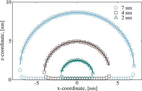
Figure 3: Shapes of droplets with radii of ca. $2$, $4$ and $7\mathrm{nm}$ (symbols) and the corresponding fits of their upper parts with a spherical cap (solid lines). The contact angle $\Theta_{\textrm{flat}}$ then results from the fit parameters.

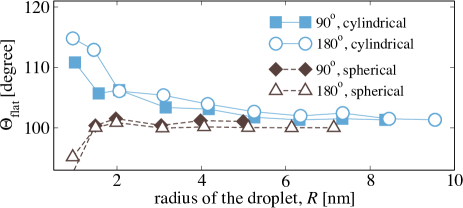
Figure 4: Comparison of the contact angle of cylindrical (two-dimensional) and spherical (3D) droplets on a flat substrate of $\tilde{\epsilon}=150\,(\mathrm{nm})^{-3}$ as a function of the droplet’s radius, $R$. Initial configurations with contact angle of $180^{\circ}$ (full cylinder and sphere) and $90^{\circ}$ (half-cylinder and semi-sphere) are utilized.

After relaxation to the equilibrium shape, we measure the contact angle. To this end, we first obtain a two-dimensional $xz$-density map in a plane through the droplet’s center of mass. Then, the liquid-vapor interface is localized according to the criterion $\rho=(\rho_{\textrm{l}}+\rho_{\textrm{v}})/2$. As an example, Fig. 3 presents the resulting shapes of drops of various sizes. To avoid uncertainties near the substrate, we apply a spherical-cap approximation to the upper part of the shapes (solid lines in Fig. 3). We thus obtain fitted radii and fitted positions of the circles’ centers, from which the contact angles can be directly inferred.

As an example of the extrapolation to infinite droplet size, we present in Fig. 4 the $\Theta_{\textrm{flat}}$ data for $\tilde{\epsilon}=150\,(\mathrm{nm})^{-3}$, for both cylindrical and spherical drops, and the two initial configurations that we studied. For the other amplitudes $\tilde{\epsilon}$ the behavior is similar. As the contact angle converges from above for cylinders, and from below for spheres, the extrapolated value can be obtained fairly accurately. Data for radii $\leq 3\,\mathrm{nm}$ should be discarded, since in this regime the fitting procedure becomes rather unreliable. This is hardly surprising, in view of the interfacial thickness of $1\,\mathrm{nm}$. Conversely, for radii $\geq 6\,\mathrm{nm}$ the asymptotic behavior is essentially reached. Averaging over these large droplets, we obtain $\Theta_{\textrm{flat}}=101.26^{\circ}$ and $120.03^{\circ}$ for $\tilde{\epsilon}=150\,(\mathrm{nm})^{-3}$ and $100\,(\mathrm{nm})^{-3}$, respectively. In the following, we refer to these values as $100^{\circ}$ and $120^{\circ}$ for simplicity. Our study therefore spans a region from weakly to moderately strongly hydrophobic substrate materials.

III.2 Corrugated substrates

Figure 5: (color online) The parameters of the substrate of striped (left) and pillared (right) corrugation type. The converged snapshots represent Cassie (left) and Wenzel (right) states. Parts of the corrugations re-enter the calculation box through periodic boundary conditions.

For striped surfaces, the fraction $f$ of surface that is covered with liquid in the Cassie state is obviously given by $c_{x}/a$. Furthermore, the contour length of the three-phase line is given by $L_{\rm c}=2L_{y}$, while the total area $A$ is $A=aL_{y}$ (see Fig. 5, left). The force-balance equation, Eq. (2), can hence be re-written as

$$\frac{c_{x}}{a}=\frac{b}{a}\cos\Theta_{\textrm{max}}+1;\;\;\;\;b=\frac{2\gamma}{P^{\rm max}}.$$ (29)

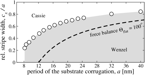
(a)

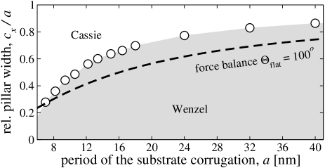
(b)

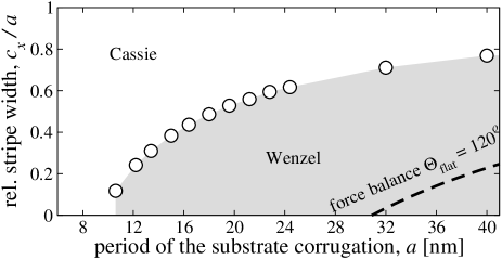
(c)

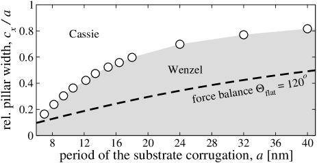
(d)

Figure 6: State diagrams presenting the boundary between Cassie and Wenzel states, for striped (panels (a) and (c)) and pillared (panels (b) and (d)) substrates. The interaction strengths are $\tilde{\epsilon}=150\,(\mathrm{nm})^{-3}$ (panels (a) and (b)), and $\tilde{\epsilon}=100\,(\mathrm{nm})^{-3}$ (panels (c) and (d)). Open circles mark the limit of metastability of the Cassie state as calculated from DFT. The shaded regions in the lower right corners of the diagrams correspond to absolute stability of the Wenzel state. In the remaining white regions the Cassie state is either stable or metastable. Black dashed lines mark the corresponding limit of metastability as calculated from the macroscopic force-balance relation, employing the respective Young contact angle on a flat substrate of $\Theta_{\textrm{flat}}=100^{\circ}$ (panels (a) and (b)), and $\Theta_{\textrm{flat}}=120^{\circ}$ (panels (c) and (d)). In all cases the hydrostatic pressure is $P^{\rm max}\simeq 50\,\mathrm{atm}$.

Similarly, for pillars (Fig. 5 right) we have $f=c_{x}^{2}/a^{2}$, $L_{\rm c}=4c_{x}$, $A=a^{2}$ and hence in this case Eq. (2) is re-written as

$$\frac{c_{x}}{a}=\frac{b}{a}\cos\Theta_{\textrm{max}}+\sqrt{\left(\frac{b}{a}\cos\Theta_{\textrm{max}}\right)^{2}+1}$$ (30)

(meaning of $b$ as above).

In order to test these relations, we pursue the following strategy: We impose the boundary condition $\rho_{\textrm{top}}=33.40\,(\mathrm{nm})^{-3}$ at the top of the calculation box (cf. Sec. II.4). We then evaluate the stress tensor, Eq. (15), at the top layer. Since the profile is rather flat at the top layer, the contribution $\propto\kappa$ can safely be neglected. Hence

$$\left.\frac{\tensor{\Pi}}{k_{B}T}\right|_{\rm top}=P_{\rm bulk}(\rho_{\rm top})\tensor{1},$$ (31)

and therefore we effectively impose a boundary condition of constant pressure at the top surface, at a value of $P\simeq 50\,\mathrm{atm}$. This is much larger than the gas pressure at the bottom, which is of order $10^{-2}\mathrm{atm}$. For this reason, we can safely identify the pressure at the top surface with the excess pressure that enters Eq. (2). We then systematically vary $c_{x}$ at constant $a$, starting with a fairly large value of $c_{x}$. In this regime, the Cassie state is stable. Upon decreasing $c_{x}$, a critical value is reached at which the Cassie state collapses and rather the Wenzel state is observed. Obviously, our calculations permit us to directly monitor this process. Our iteration scheme starts with an interface located $\sim 1\,\mathrm{nm}$ above the top of the asperities; therefore the procedure is expected to always converge to the (possibly metastable) Cassie state, unless it is absolutely unstable. It should be recalled that the purpose of the investigation is to find this limit of metastability. Finally, this procedure is repeated for various values of $a$, resulting in a state diagram in the plane $a$ vs. $c_{x}/a$. If the phenomenological force balance holds, then the transition line must be given by Eq. (29) for stripes, and by Eq. (30) for pillars.

At this point, it should be noted that the parameters that enter the force-balance relation are (i) the geometry data (input data of the calculations), (ii) the pressure and the interfacial tension (known accurately, see also end of Sec. II.2), and (iii) the contact angle $\Theta_{\textrm{max}}$, which is not known. Due to the diffuse nature of the interface and the nanoscopic corrugation dimensions it is practically impossible to obtain a contact angle directly from the simulation data. We therefore pursue the following two strategies to do the comparison: (i) On the one hand, we simply assume that the relevant contact angle is just the Young value $\Theta_{\textrm{flat}}$ as follows from macroscopic considerations (cf. Appendix A), and check how well the predicted transition line matches the DFT result. This strategy relies on the macroscopic assumption that contact angle hysteresis is of no importance for ideal substrates, which has been demonstrated to be valid at least for some systems Khare et al. (2007); Herminghaus, Brinkmann, and Seemann (2008). (ii) On the other hand, we solve the force-balance relation, Eq. 2, for $\Theta_{\textrm{max}}$. We can hence determine the contact angle as an effective parameter, to be evaluated along the DFT phase transition line.

The results of this analysis are summarized in Figs. 6 and 7. The state diagrams in Fig. 6 clearly show that the force-balance relation gives a qualitatively reasonable description of the Cassie-Wenzel transition even on the nanoscale. However, the attempt to describe the phenomenon quantitatively by just employing the Young contact angle (black dashed lines) fails. The deviations increase systematically with increasing hydrophobicity, as clearly shown in Fig. 7, plotting our resulting effective contact angles $\Theta_{\rm max}$ as a function of the substrate period $a$ for various $\tilde{\epsilon}$. The effective angles are smaller than the corresponding Young angles and the discrepancy grows significantly with increasing hydrophobicity.

We therefore believe that it is reasonable to assume that our effective contact angles embody the effects of (i) the finite range of the substrate potential, (ii) finite width of the liquid-vapor interface, and (iii) line tension.

Interestingly, the details of the geometry seem to play only a minor role: At fixed hydrophobicity the effective $\Theta_{\textrm{max}}$ is practically constant in the case of stripes. Even more importantly, the pillared geometry yields the same effective contact angle for large periods of substrate corrugation ($a\gtrsim 20\,\textrm{nm}$), if only the hydrophobicity is the same, validating assumption (iii). We believe that the deviations for smaller values of $a$ are due to the effect of the pillar corners, whose relative importance decreases with increasing corrugation dimensions.

Another remarkable observation is the finding that in the semi-macroscopic limit ($a\gtrsim 20\,\textrm{nm}$) the effective $\Theta_{\textrm{max}}$ values are fairly similar even for different hydrophobicities, and deviate much less from each other than the corresponding Young angles. Even though at these scales the contact angles are usually considered as macroscopic ones, we emphasize that the height of the corrugation, $2\,\textrm{nm}$, is nanoscopic, and this may possibly trigger this effect. In our model hydrophobicity (in other words, surface “chemistry”) is varied by modifying $\tilde{\epsilon}$, i. e. the energy scale of the attraction, while $\sigma$, the characteristic length scale affecting the atomic-scale corrugation, remains unchanged. Apparently, on this level of description, the phenomenon of super-hydrophobicity is governed more by geometrical effects and the range of the substrate potential rather than by the strength of attraction.

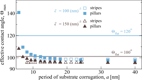
Figure 7: (color online) The effective contact angle $\Theta_{\textrm{max}}$ for the force-balance relation as a function of the period of the substrate corrugation $a$, which we use to parameterize the path along the Cassie-Wenzel transition line.

III.3 Considerations on the absence of thermal fluctuations

An important question refers to the extent to which the generality of our conclusions is affected by the absence of fluctuations in classical DFT. Above the length scales where microscopic roughness of the interface sets in, a qualitative estimate regarding the role of fluctuations can be obtained from capillary-wave theory von Smoluchowski (1908); Buff, Lovett, and Stillinger (1965) and its application to fluctuating interfaces Werner et al. (1999); Vink, Horbach, and Binder (2005); Ismail, Grest, and Stevens (2006); Sedlmeier, Horinek, and Netz (2009). According to this theory, the mean square deviation of the local interface position from its average location is given by $s^{2}=\frac{k_{B}T}{2\gamma}\ln\left(\frac{L}{B_{\rm o}}\right)$, where $L$ is the lateral size of the free interface between corrugations. $B_{\rm o}$ stands for a coarse-graining scale Werner et al. (1999) below which the capillary-wave Hamiltonian is not applicable, being of the order of one nanometer (e. g. Ref. Sedlmeier, Horinek, and Netz, 2009 reported a crossover at $B_{\rm o}=0.8\,\mathrm{nm}$). We thus find that for the parameters studied in this paper ($L$ of the order of a few tens of nanometers, and assuming $B_{\rm o}=1\,\mathrm{nm}$) the fluctuation $s$ remains on the sub-nanometer scale. This estimate suggests that at least long-wave fluctuations should not cause significant deviations from the observations reported here.

IV Summary and outlook

The applicability of a phenomenological force-balance relation for the Cassie-Wenzel transition of a water-vapor interface has been studied by a simple model based upon classical DFT. The method allows to study arbitrary surface geometries on the nanoscale, where the phenomenological picture is least obviously valid. In the present paper we picked corrugations of striped and pillared type.

The macroscopic force-balance relation describes the absolute stability of the Cassie state in terms of the impalement pressure that depends on geometrical parameters of the corrugation, the liquid-vapor interface tension, and the effective contact angle, $\Theta_{\textrm{max}}$. An attempt to interpret this angle as the Young contact angle fails on the nanoscale. Instead, the effective angle quantitatively satisfying the force-balance is smaller than the corresponding Young’s value and takes into account effects of the finite range of the liquid-solid interactions, line tension and the diffuse nature of the interface. This suggestion is corroborated by the fact that in the case of striped geometry the effective contact angle is independent of the substrate period. Furthermore, for large periods ($a\gtrsim 20\,\textrm{nm}$) the effective contact angles found for striped and pillared geometry are the same at fixed hydrophobicity, as the influence of the corners of the pillars is not too large. We do not find any indication that the Cassie-Wenzel transition can be of second order at least for some nanoscopic geometries and hydrophobicity strengths, as was suggested in Ref. Tretyakov and Müller, 2013. However in that latter study thermal fluctuations were present and probably played a crucial role in the transition.

In the present investigation we employed a simple classical DFT model which captures the long-wavelength properties of a liquid, while neglecting local-scale packing. The latter can be taken into account through more elaborate DFT descriptions. We expect that such local packing will result in a certain shift of the predicted effective angle in two- and three-dimensional geometries, even if the macroscopic thermodynamics remains unchanged. However, we also expect that (at fixed hydrophobicity) these very different geometries will be still characterized by a unique value of the effective angle, provided that the corrugation features are not too strongly miniaturized. A test of this hypothesis is left for future work; within the framework of the present model this is (at least conceptually) easy to do by implementing more advanced density functionals. Further possible extensions include the incorporation of a gas component (air instead of water vapor) as well as numerical improvements, such as adaptive-mesh schemes, to reach scales relevant to the range of optical observations in experiments.

Appendix A Macroscopic theory of the Cassie-Wenzel transition

We here derive the critical excess pressure for the Cassie-Wenzel transition. Figure 8 outlines a simple geometry that is easy to analyze.

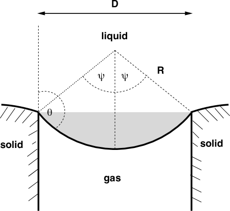
Figure 8: Simple macroscopic geometry for a liquid on a structured surface in the Cassie state.

We assume that the situation is translationally invariant in the $y$ direction, i. e. the direction perpendicular to the drawing plane. We assume that the system has an extension $L_{y}$ in that direction. We furthermore assume, for simplicity, that the gas–liquid interface has the shape of a cylinder surface. Finally, we assume that the gas–solid interfaces are perpendicular to the (overall) surface, and that the asperities are so deep that effects of their finite depth (“sagging”) can be ignored. The figure then shows the liquid suspended in the Cassie state. We denote the lateral extension of the cavity with $D$. It is related to the cylinder radius $R$ and the opening angle $2\psi$ via

$$\frac{D}{2}=R\sin\psi,$$ (32)

while the effective contact angle $\Theta$ (as defined in the figure) is given by

$$\Theta=\psi+\frac{\pi}{2}$$ (33)

(we use radians as units for angles). The area of the gas–liquid interface is then given by

$$A=L_{y}\,R\,2\psi=L_{y}D\frac{\psi}{\sin\psi},$$ (34)

while the liquid volume corresponding to the shaded area of the figure is given by

$$V_{\rm l} = L_{y}\left(R^{2}\psi-R\sin\psi\,R\cos\psi\right)$$ (35)

$$= \frac{L_{y}D^{2}}{4\sin^{2}\psi}\left(\psi-\sin\psi\cos\psi\right).$$

If we denote the total volume of the cavity with $V_{\rm tot}$, then the volume occupied by the gas, $V_{\rm g}$, is obviously given by

$$V_{\rm g}=V_{\rm tot}-V_{\rm l}.$$ (36)

We now consider the grand potential of the system within the total volume of the cavity. The bulk contributions are given by

$$\Omega^{\rm bulk}=-P_{\rm l}V_{\rm l}-P_{\rm g}V_{\rm g},$$ (37)

where $P_{\rm l}$ and $P_{\rm g}$ are the pressures in the liquid and gas phases, respectively. As a result of the curved interface, these pressures are not the same (Laplace pressure). We then can define an excess grand potential (using the gas phase fully occupying the cavity as a reference state) via

$$\Omega^{\rm bulk}_{\rm ex}=\Omega^{\rm bulk}+P_{\rm g}V_{\rm tot}=-P_{\rm ex}V_{\rm l},$$ (38)

where the excess pressure is given by

$$P_{\rm ex}=P_{\rm l}-P_{\rm g}.$$ (39)

The full excess grand potential has also an interface contribution, such that

$$\Omega_{\rm ex}=\gamma_{\rm lg}A-P_{\rm ex}V_{\rm l},$$ (40)

where $\gamma_{\rm lg}$ is the liquid-gas interface tension.

Normalizing the potential by the factor $D^{2}L_{y}$, we thus obtain for the normalized potential of the Cassie state

$$\omega_{\rm C}=\Gamma_{\rm lg}\frac{\psi}{\sin\psi}-P_{\rm ex}\frac{1}{4\sin^{2}\psi}\left(\psi-\sin\psi\cos\psi\right),$$ (41)

where $\Gamma_{\rm lg}=\gamma_{\rm lg}/D$.

The equilibrium shape of the interface in the Cassie state is then obtained by minimizing $\omega_{\rm C}$ with respect to $\psi$. After some straightforward (computer) algebra, this results in

$$\sin\psi=\frac{P_{\rm ex}}{2\Gamma_{\rm lg}},$$ (42)

or, returning to the angle $\Theta$,

$$-\cos\Theta=\frac{P_{\rm ex}}{2\Gamma_{\rm lg}}.$$ (43)

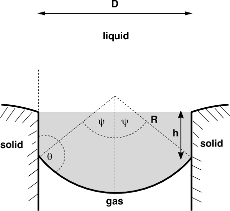
Figure 9: Macroscopic geometry for a liquid penetrating the cavity. The depth of the penetration is $h$.

In order to study the stability of the Cassie state, we compare its grand potential with the grand potential of a Wenzel-like state, where the interface is pushed into the cavity by some amount $h$ (Fig. 9). For this latter potential we obtain

$$\Omega_{\rm W} = \Omega_{\rm C}-P_{\rm ex}DL_{y}h+2\left(\gamma_{\rm sl}-\gamma_{\rm sg}\right)L_{y}h,$$ (44)

$$\omega_{\rm W} = \omega_{\rm C}-\left(P_{\rm ex}-2\Delta\Gamma\right)\frac{h}{D}.$$ (45)

The second term corresponds to the additional bulk contribution from the additional liquid that has been pushed into the cavity. Similarly, the third term is the interface contribution, where $\gamma_{\rm sl}$ and $\gamma_{\rm sg}$ are the interface tensions of the solid-liquid and solid-gas interfaces, respectively. The difference of these values occurs since a solid-gas interface is replaced with a solid-liquid interface. In the second equation, we abbreviate $\Delta\Gamma=\left(\gamma_{\rm sl}-\gamma_{\rm sg}\right)/D$.

The equilibrium configuration is then obtained by optimizing $\omega_{\rm W}$ with respect to both $\psi$ and $h$. Therefore, $\psi$ remains unchanged, compared to the Cassie state, while the solution for $h$ depends on the applied pressure. For $P_{\rm ex}<2\Delta\Gamma$ we obtain $h=0$, i. e. for small pressures the Cassie state remains stable. Conversely, for $P_{\rm ex}>2\Delta\Gamma$ the solution is $h=\infty$, which corresponds to the Wenzel state.

The critical pressure (or the maximum excess pressure up to which the Cassie state is stable) is therefore given by

$$P^{\rm max}=2\Delta\Gamma.$$ (46)

Inserting this into Eq. (43), we find for the contact angle at the transition

$$-\cos\Theta=\frac{\Delta\Gamma}{\Gamma_{\rm lg}}$$ (47)

or

$$\gamma_{\rm sg}=\gamma_{\rm sl}+\gamma_{\rm lg}\cos\Theta,$$ (48)

which is Young’s equation. In other words, the Cassie-Wenzel transition occurs precisely when the contact angle has reached the Young value, $\Theta=\Theta_{\textrm{flat}}$. Therefore, the critical pressure can also be written as

$$P^{\rm max}=-2\Gamma_{\rm lg}\cos\Theta_{\textrm{flat}}=-\frac{2\gamma_{\rm lg}}{D}\cos\Theta_{\textrm{flat}},$$ (49)

which is the formula given in the main text.

References

- Yao, Song, and Jiang (2011) X. Yao, Y. L. Song, and L. Jiang, Adv. Mater. 23, 719 (2011).
- Park et al. (2013) K. C. Park, S. S. Chhatre, S. Srinivasan, R. E. Cohen, and G. H. McKinley, Langmuir 29, 13269 (2013).
- Watanabe and Udagawa (2001) K. Watanabe and H. Udagawa, AIChE J. 47, 256 (2001).
- Gogte et al. (2005) S. Gogte, P. Vorobieff, R. Truesdell, A. Mammoli, F. van Swol, P. Shah, and C. J. Brinker, Phys. Fluids 17, 051701 (2005).
- Drappier et al. (2006) J. Drappier, T. Divoux, Y. Amarouchene, F. Bertrand, S. Rodts, O. Cadot, J. Meunier, and D. Bonn, Europhys. Lett 74, 362 (2006).
- Ou, Perot, and Rothstein (2004) J. Ou, B. Perot, and J. P. Rothstein, Phys. Fluids 16, 4635 (2004).
- McHale, Newton, and Shirtcliffe (2010) G. McHale, M. I. Newton, and N. J. Shirtcliffe, Soft Matter 6, 714 (2010).
- Paven et al. (2013) M. Paven, P. Papadopoulos, S. Schottler, X. Deng, V. Mailander, D. Vollmer, and H.-J. Butt, Nat. Commun. 4, 2512 (2013).
- Cassie and Baxter (1944) A. B. D. Cassie and S. Baxter, Trans. Faraday Soc. 40, 546 (1944).
- Bormashenko (2015) E. Bormashenko, Adv. Colloid Interface Sci. 222, 92 (2015).
- Callies and Quéré (2005) M. Callies and D. Quéré, Soft Matter 1, 55 (2005).
- Dorrer and Rühe (2009) C. Dorrer and J. Rühe, Soft Matter 5, 51 (2009).
- Nosonovsky and Bhushan (2007) M. Nosonovsky and B. Bhushan, Nano Lett. 7, 2633 (2007).
- Wenzel (1936) R. N. Wenzel, Industrial & Engineering Chemistry 28, 988 (1936).
- Extrand (2002) C. W. Extrand, Langmuir 18, 7991 (2002).
- Zheng, Yu, and Zhao (2005) Q. S. Zheng, Y. Yu, and Z. H. Zhao, Langmuir 21, 12207 (2005).
- Bartolo et al. (2006) D. Bartolo, F. Bouamrirene, E. Verneuil, A. Buguin, P. Silberzan, and S. Moulinet, Europhys. Lett. 74, 299 (2006).
- Cottin-Bizonne et al. (2004) C. Cottin-Bizonne, C. Barentin, E. Charlaix, L. Bocquet, and J.-L. Barrat, Eur. Phys. J. E 15, 427 (2004).
- Moulinet and Bartolo (2007) S. Moulinet and D. Bartolo, Eur. Phys. J. E 24, 251 (2007).
- Butt, Vollmer, and Papadopoulos (2014) H.-J. Butt, D. Vollmer, and P. Papadopoulos, Adv. Colloid Interface Sci. (2014), http://dx.doi.org/10.1016/j.cis.2014.06.002.
- Hemeda and Tafreshi (2014) A. A. Hemeda and H. V. Tafreshi, Langmuir 30, 10317 (2014).
- de Gennes, Brochard-Wyart, and Quéré (2004) P. de Gennes, F. Brochard-Wyart, and D. Quéré, Capillarity and Wetting Phenomena (Springer, 2004).
- Extrand (2006) C. W. Extrand, Langmuir 22, 1711 (2006).
- Checco et al. (2014) A. Checco, B. M. Ocko, A. Rahman, C. T. Black, M. Tasinkevych, A. Giacomello, and S. Dietrich, Phys. Rev. Lett. 112, 216101 (2014).
- Marmur (2004) A. Marmur, Langmuir 20, 3517 (2004).
- Patankar (2004) N. A. Patankar, Langmuir 20, 7097 (2004).
- Dupuis and Yeomans (2005) A. Dupuis and J. M. Yeomans, Langmuir 21, 2624 (2005).
- Gross et al. (2010) M. Gross, F. Varnik, D. Raabe, and I. Steinbach, Phys. Rev. E 81, 051606 (2010).
- Ren (2014) W. Ren, Langmuir 30, 2879 (2014).
- Giacomello et al. (2015) A. Giacomello, S. Meloni, M. Müller, and C. M. Casciola, J. Chem. Phys. 142, 104701 (2015).
- Savoy and Escobedo (2012) E. S. Savoy and F. A. Escobedo, Langmuir 28, 16080 (2012).
- Evans (1979) R. Evans, Adv. Phys. 28, 143 (1979).
- Dietrich (1988) S. Dietrich, in Phase Transitions and Critical Phenomena, edited by C. Domb and J. L. Lebowitz, Vol. 12 (Academic Press, 1988).
- Tarazona, Marconi, and Evans (1987) P. Tarazona, U. M. B. Marconi, and R. Evans, Mol. Phys. 60, 573 (1987).
- Wu (2006) J. Wu, AIChE J. 52, 1169 (2006).
- Weeks, Vollmayr, and Katsov (1997) J. D. Weeks, K. Vollmayr, and K. Katsov, Physica A 244, 461 (1997).
- Cahn and Hilliard (1958) J. W. Cahn and J. E. Hilliard, J. Chem. Phys. 28, 258 (1958).
- Tarazona (1985) P. Tarazona, Phys. Rev. A 31, 2672 (1985).
- Lum, Chandler, and Weeks (1999) K. Lum, D. Chandler, and J. D. Weeks, J. Phys. Chem. B 103, 4570 (1999).
- Hughes, Krebs, and Roundy (2013) J. Hughes, E. J. Krebs, and D. Roundy, J. Chem. Phys. 138, 024509 (2013).
- Yang et al. (1992) B. Yang, D. E. Sullivan, B. Tjipto-Margo, and C. G. Gray, Mol. Phys. 76, 709 (1992).
- Yang, Sullivan, and Gray (1994) B. Yang, D. E. Sullivan, and C. G. Gray, J. Phys.: Condens. Matter 6, 4823 (1994).
- Clark et al. (2006) G. N. I. Clark, A. J. Haslam, A. Galindo, and G. Jackson, Mol. Phys. 104, 3561 (2006).
- Lischner and Arias (2010) J. Lischner and T. A. Arias, J. Phys. Chem. B 114, 1946 (2010).
- Sundararaman, Letchworth-Weaver, and Arias (2012) R. Sundararaman, K. Letchworth-Weaver, and T. A. Arias, J. Chem. Phys. 137, 044107 (2012).
- Koch, Dietrich, and Napiórkowski (1995) W. Koch, S. Dietrich, and M. Napiórkowski, Phys. Rev. E 51, 3300 (1995).
- Malijevský (2014) A. Malijevský, J. Chem. Phys. 141, 184703 (2014).
- Berim and Ruckenstein (2015) G. O. Berim and E. Ruckenstein, Nanoscale 7, 7873 (2015).
- Zhang and Ren (2014) Y. Zhang and W. Ren, J. Chem. Phys. 141, 244705 (2014).
- Yang, Fleming, and Gibbs (1976) A. J. M. Yang, P. D. Fleming, and J. H. Gibbs, J. Chem. Phys. 64, 3732 (1976).
- Anderson, McFadden, and Wheeler (1998) D. M. Anderson, G. B. McFadden, and A. A. Wheeler, Annu. Rev. Fluid. Mech. 30, 139 (1998).
- Thompson (2006) R. B. Thompson, Phys. Rev. E 73, 020502 (2006).
- Müller, MacDowell, and Yethiraj (2003) M. Müller, L. G. MacDowell, and A. Yethiraj, J. Chem. Phys. 118, 2929 (2003).
- Bryk and MacDowell (2008) P. Bryk and L. G. MacDowell, J. Chem. Phys. 129, 104901 (2008).
- Landau and Lifshitz (1975) L. D. Landau and E. M. Lifshitz, The Classical Theory of Fields, 4th ed., Course of Theoretical Physics, Vol. 2 (Pergamon Press, 1975).
- Lide (2004) D. R. Lide, CRC Handbook of Chemistry and Physics, 85th ed. (Taylor & Francis, 2004).
- Jones and Richards (1999) R. A. L. Jones and R. W. Richards, Polymers at Surfaces and Interfaces (Cambridge University Press, 1999).
- Landau and Lifshitz (1976) L. D. Landau and E. M. Lifshitz, Mechanics, 3rd ed., Course of Theoretical Physics, Vol. 1 (Butterworth-Heinemann, 1976).
- Kayser (1976) W. V. Kayser, J. Colloid Interface Sci. 56, 622 (1976).
- Sedlmeier, Horinek, and Netz (2009) F. Sedlmeier, D. Horinek, and R. R. Netz, Phys. Rev. Lett. 103, 136102 (2009).
- Berim and Ruckenstein (2008) G. O. Berim and E. Ruckenstein, J. Chem. Phys. 129, 014708 (2008).
- Biben and Joly (2008) T. Biben and L. Joly, Phys. Rev. Lett. 100, 186103 (2008).
- Steele (1973) W. A. Steele, Surf. Sci 36, 317 (1973).
- Mansfield and Theodorou (1991) K. F. Mansfield and D. N. Theodorou, Macromolecules 24, 4295 (1991).
- Drolet and Fredrickson (2001) F. Drolet and G. H. Fredrickson, Macromolecules 34, 5317 (2001).
- Müller and Schmid (2005) M. Müller and F. Schmid, Adv. Polym. Sci. 185, 1 (2005).
- Fredrickson, Ganesan, and Drolet (2002) G. H. Fredrickson, V. Ganesan, and F. Drolet, Macromolecules 35, 16 (2002).
- Jr. Anderson (1995) J. D. Jr. Anderson, Computational Fluid Dynamics (McGraw-Hill, Inc, 1995).
- William H. Press and Flannery (2007) W. T. V. William H. Press, Saul A. Teukolsky and B. P. Flannery, Numerical Recipes. The Art of Scientific Computing, 3rd ed. (Cambridge University Press, 2007).
- Tretyakov (2015) N. Tretyakov, “mf_dft_water code,” GitHub repository: https://github.com/niktre/mf_dft_water.git (2015).
- Binder et al. (2011) K. Binder, B. Block, S. K. Das, P. Virnau, and D. Winter, J. Stat. Phys. 144, 690 (2011).
- Khare et al. (2007) K. Khare, M. Brinkmann, B. M. Law, E. L. Gurevich, S. Herminghaus, and R. Seemann, Langmuir 23, 12138 (2007).
- Herminghaus, Brinkmann, and Seemann (2008) S. Herminghaus, M. Brinkmann, and R. Seemann, Ann. Rev. Mat. Res. 38, 101 (2008).
- von Smoluchowski (1908) M. von Smoluchowski, Ann. d. Phys. 330, 205 (1908).
- Buff, Lovett, and Stillinger (1965) F. Buff, R. Lovett, and F. Stillinger, Phys. Rev. Lett. 15, 621 (1965).
- Werner et al. (1999) A. Werner, F. Schmid, M. Müller, and K. Binder, Phys. Rev. E 59, 728 (1999).
- Vink, Horbach, and Binder (2005) R. L. C. Vink, J. Horbach, and K. Binder, J. Chem. Phys. 122, 134905 (2005).
- Ismail, Grest, and Stevens (2006) A. E. Ismail, G. S. Grest, and M. J. Stevens, J. Chem. Phys. 125, 014702 (2006).
- Tretyakov and Müller (2013) N. Tretyakov and M. Müller, Soft Matter 9, 3613 (2013).