Derivative pricing as a transport problem: MPDATA solutions to Black-Scholes-type equations

Abstract

We discuss in this note applications of the Multidimensional Positive Definite Advection Transport Algorithm (MPDATA) to numerical solutions of partial differential equations arising from stochastic models in quantitative finance. In particular, we develop a framework for solving Black-Scholes-type equations by first transforming them into advection-diffusion problems, and numerically integrating using an iterative explicit finite-difference approach, in which the Fickian term is represented as an additional advective term. We discuss the correspondence between transport phenomena and financial models, uncovering the possibility of expressing the no-arbitrage principle as a conservation law. We depict second-order accuracy in time and space of the embraced numerical scheme. This is done in a convergence analysis comparing MPDATA numerical solutions with classic Black-Scholes analytical formulæ for the valuation of European options. We demonstrate in addition a way of applying MPDATA to solve the free boundary problem (leading to a linear complementarity problem) for the valuation of American options. We finally comment on the potential the MPDATA framework has with respect to being applied in tandem with more complex models typically used in quantitive finance.

Introduction

MPDATA stands for Multidimensional Positive Definite Advection Transport Algorithm. The algorithm was introduced in [1, 2] as a robust numerical scheme for atmospheric modelling applications. Thanks to continued research, extensions, and generalisations of MPDATA (see MPDATA review papers [3, 4]), it has been applied in a wide range of computational research for numerical integration of partial differential equations describing transport phenomena. Applications include modelling of brain injuries, transport in porous media, sand dune formation, convective cloud systems, operational weather prediction, and studies of climate dynamics and solar magnetohydrodynamics (refer to [5, sec. 1.2] for a recent review of applications).

The Black-Scholes model [6] is a mathematical description of the behaviour of financial markets in which trading occurs in financial assets, as well as derivative financial instruments - contracts whose values are dependent on prices of other assets. The model gives rise to formulæ routinely used in the financial industry to price derivatives. The 1997 Nobel Prize in economic sciences was awarded to contributors to this pricing methodology, Robert Merton and Myron Scholes.

The goal of this paper is twofold. First, we wish to attract the mostly-geoscientific MPDATA community to applications in quantitative finance, a domain replete with applications of finite-difference methods (see, e.g., [7]). Second, we intend to turn the attention of the quantitative finance community to a family of accurate finite-difference solvers possessing characteristics that are advantageous in tackling derivative pricing problems: conservativeness, high-order accuracy, low numerical diffusion, and monotonicity-preserving oscillation-free solutions. This is in line with the proposal put forward in [8] to investigate robust and effective numerical schemes documented in the computational fluid dynamics literature as alternatives to commonly used numerical schemes in financial engineering, with the aim of “improving the finite difference methods gene pool as it were.” To these ends, leveraging the mathematical equivalence between Black-Scholes-type models and transport models, we detail applications of MPDATA to numerically reproduce the analytical solution of a celebrated benchmark problem — the Black-Scholes formula for pricing of European options — and to numerically solve the associated free boundary problem arising in the valuation of American options.

With the aim of catering to both communities, we begin this note with a brief introduction to both the Black-Scholes model and the MPDATA solver. We purposefully include explanations of terms that can be considered elementary in their respective domains. Also included is a discussion of the variable transformation that converts the Black-Scholes equation into a homogeneous advection-diffusion equation. The background section is followed by a description of a sample application of MPDATA for pricing a financial instrument composed of European options. First, we detail the numerical solution procedure, and discuss the results for a single simulation. Second, we corroborate results of multiple simulations with analytical solutions in an analysis quantifying the rate of convergence of the numerical solutions for both upwind and MPDATA schemes. We conclude this note by highlighting the potential MPDATA has for further applications in finance. In the appendix, we present an extension of the developed framework for pricing American options.

Background

The Black-Scholes model in a nutshell

A common ansatz in financial market modelling is that the price $S$ of an asset follows a continuous-time lognormal diffusion process known as geometric Brownian motion. This process is modelled by the stochastic differential equation (SDE):

$$dS=S(\mu dt+\sigma dw)$$ (1)

where $\mu$ and $\sigma$ are constants denoting the expected instantaneous return on investment in the asset and the asset price volatility, respectively, $t$ denotes time and $w$ is a Wiener process (also called a Brownian motion). This simple model embodies the fact that what matters to investors is the rate of return on their investment in an asset, and not the change in the asset price (in which case, the $S$ term would be dropped from the right-hand side of eq. 1 as in the Bachelier model [10], a seminal fin-de-siècle starting point for mathematical finance and, it is noteworthy, a seminal work in the theory of Brownian motion itself; for discussion see [11]). Furthermore, this model entails two propositions: (i) in the limit where the volatility is negligible, the investment in the asset mimics a deposit with interest rate $\mu$; (ii) in the opposite limit where $\mu$ is negligible, the return on the investment is random with a normal distribution.

The Black-Scholes model assumes that the modelled asset price follows a geometric Brownian motion. Key among the other model assumptions are that the rate of return on a riskless investment is fixed and given by the so-called “risk-free interest rate” (a high-rated government bond can be thought of as a surrogate for the idealised riskless investment), and that there are no arbitrage opportunities (precluding the possibility of riskless returns in excess of the the risk-free interest rate).

Suppose, in the Black-Scholes model, that a derivative instrument is also traded in the market. For instance, a “European call option” on an asset (e.g., a stock) is a type of a derivative that gives its holder the right, but not an obligation, to purchase the underlying asset on a specified future date at a specified price. An American option differs from a European option only in that it can be exercised at any time prior to its date of expiration (cf. Appendix). Given an asset in the Black-Scholes model whose price process is given by $S$, the aim is to discover the price of a derivative contingent on $S$.

Let $f(S,t)$ be the value of an option dependent on the asset price $S$ at time $t$. Since $S$ follows a Wiener process, the change in $f$ can be expressed using Itô’s lemma as:

$$df=\left(\frac{\partial f}{\partial t}+\mu S\frac{\partial f}{\partial S}+\frac{1}{2}\sigma^{2}S^{2}\frac{\partial^{2}f}{\partial S^{2}}\right)dt+\sigma S\frac{\partial f}{\partial S}dw$$ (2)

The crucial observation is that the asset price $S$ and the option value $f$ have the same source of randomness, associated with the Wiener process $w$. Thus, one can construct a suitably weighted portfolio by selling one unit of the option and holding as much, $\Delta_{t}$, of the underlying asset so as to eliminate the randomness and make the portfolio riskless. In finance, risk reduction is referred to as hedging. The portfolio value $\Pi(S,t)$ is given by

$$\Pi=-f+\Delta_{t}S$$ (3)

Substituting from eq. (1) and eq. (2), we have

$$-df+\Delta_{t}dS=\left[-\frac{\partial f}{\partial t}-\frac{1}{2}\sigma^{2}S^{2}\frac{\partial^{2}f}{\partial S^{2}}+\left(\Delta_{t}-\frac{\partial f}{\partial S}\right)\mu S\right]dt+\left(\Delta_{t}-\frac{\partial f}{\partial S}\right)\sigma Sdw$$

showing that the only stochastic contribution to the portfolio value at time $t$ is given by $\int_{0}^{t}\left(\Delta_{u}-\frac{\partial f}{\partial S_{u}}\right)\sigma S_{u}dw_{u}$. Thus, by adopting the so-called delta-hedging strategy, with the proportion $\Delta_{t}$ of the asset held at time $t$ assumed to be locally constant and equal to $\left.\frac{\partial f}{\partial S}\right|_{t}$, the portfolio is instantaneously riskless. A riskless portfolio must evolve according to the risk-free interest rate $r$:

$$d\Pi=\left(-\frac{\partial f}{\partial t}-\frac{1}{2}\sigma^{2}S^{2}\frac{\partial^{2}f}{\partial S^{2}}\right)dt=\Pi rdt$$ (4)

Substituting from eq. (3) into eq. (4) yields the celebrated Black-Scholes equation [6]:

$$\frac{\partial f}{\partial t}+rS\frac{\partial f}{\partial S}+\frac{\sigma^{2}}{2}S^{2}\frac{\partial^{2}f}{\partial S^{2}}-rf=0$$ (5)

The derivation of eq. (5) hinged on the elimination of the stochastic term, reducing the SDE to a partial differential equation (PDE). It is worth noting that there exists an alternative approach of casting the option valuation problem in PDE form via the Martingale pricing theorem, using the Kolmogorov forward equation (or Fokker-Planck equation) [12].

Derivative pricing as a transport problem

The Black-Scholes equation can be transformed into a homogeneous advection-diffusion (convection-diffusion, scalar transport) equation using the following variable substitution:

$$\left\{\begin{array}[]{llr}\psi&=e^{-rt}f(S,t)\\ x&=\ln S\\ u&=r-\frac{\sigma^{2}}{2}\\ \nu&=-\frac{\sigma^{2}}{2}\end{array}\right.$$ (6)

leading to:

$$\frac{\partial\psi}{\partial t}+u\frac{\partial\psi}{\partial x}-\nu\frac{\partial^{2}\psi}{\partial x^{2}}=0$$ (7)

The Black-Scholes methodology relies on solving a terminal value problem (hence the negative sign of $\nu$); the substitution (6) can be extended to lead to an initial value problem by introducing $\tau=T-t$ as in [13, eq. 5.68-5.71]. The connection between the Black-Scholes equation and convection-diffusion equations has been mentioned in the literature; see e.g. [14, sec. 1.1] in which the notion of “financial drift” is used.

Adapting a general technique expounded in [15, Sec. 3.2] and [16, 17] (as well as in [18] for the case of diffusion-only problem), eq. (7) can be rearranged to mimic an advection-only problem, assuming $u$ and $\nu$ constant in $x$:

$$\frac{\partial\psi}{\partial t}+\frac{\partial}{\partial x}\left[\left(u-\frac{\nu}{\psi}\frac{\partial\psi}{\partial x}\right)\psi\right]=0$$ (8)

which we will leverage in numerical solutions of eq. (7). Equations (4) and (4) followed from the no-arbitrage condition, which embodies the assumption that a riskless portfolio cannot have returns in excess of the risk-free interest rate. In eq. (8), this no-arbitrage condition is cast in the form of a conservation law.

Noteworthy, the prevalent approach to solving the Black-Scholes equation is to transform it to a heat equation, e.g. by amending the variable substitution (6) by setting $x=\ln S+(r-\sigma^{2}/2)\tau$ [13, eq. 5.72]. Such approach, which can be viewed as a transformation of the transport problem from an Eulerian into a Lagrangian frame of reference, leads to the elimination of the advective term and enables the derivation of an analytical solution of the Black-Scholes equation. In contrast, the approach embodied in eq. (8), which leads to the elimination of the Fickian term, facilitates numerical integration by not introducing time-dependent coordinate transformations and by allowing for consistent discretisation of both the advective and Fickian fluxes.

Commenting on the variable substitution (6), we note that $x=\ln(S)$ transforms the Black-Scholes equation into a constant-coefficient advection-diffusion equation with a source term. Introducing $\psi(x,t)$, in financial terms the present (discounted) value of the option, reduces the equation to a homogeneous one. This is akin to the incorporation of adiabatic cooling/heating in atmospheric heat budget equations, not through the use of a source term, but rather through the introduction of potential temperature. One may note a curious analogy in the descriptive definitions of the two quantities. Potential temperature, linked with the entropy of an ideal gas (see [19] for a historical perspective on its introduction), is commonly described as the temperature a parcel of air would have if brought adiabatically to a base level “zero”. The discounted option price $\psi$ represents the value that the option would have if brought from its state at a future time $t$ to the present time $t=0$.

Equation (7) (and its generalisations) is a staple in geoscientific research, where it is used for modelling transport phenomena. For instance, it can depict the transport in the atmosphere of a pollutant concentration field $\psi$ by wind of velocity $u$ subject to diffusion with coefficient $\nu$. In finance, the key application of eq. (7) is to solve, backwards-in-time, for the current price of the option $f(S_{0},0)=\psi(\ln(S_{0}),0)$, where $S_{0}$ is the current price of the underlying asset. The terminal condition (starting point for the solver) is given by the so-called payoff function $f(S,T)=\psi(\ln(S),T)$, defining the type of derivative contract under consideration (option to buy the asset, option to sell the asset, combination of such options, etc.).

Making a heuristic physical analogy, we note that eq. (7) in our current financial context governs the transport of the option price $f$ discounted to its present value $\psi$. The second term of eq. (7), which governs the advection of the quantity of interest, $\psi$, incorporates a velocity $u$ at which $\psi$ is moving. Noting that since the underlying process $S$ is governed by a geometric Brownian motion, and that the spatial variable in eq. (7) is $x=\ln(S)$, the solution of the geometric Brownian motion SDE (1) with $\mu=r$ implies that the drift on $x$ is precisely $(r-\frac{\sigma^{2}}{2})$ (here the replacement of $\mu$ by $r$ is justified on the grounds of risk-neutral pricing for which we omit the details). This explains the form of the advective term in eq. (7). Moreover, Itô’s lemma implies that any twice-differentiable scalar function of $S$ and $t$ will have a diffusivity coefficient precisely $\frac{\sigma^{2}}{2}$, which explains the Fickian term in eq. (7). Thus, eq. (7) could be viewed as describing the transport of the discounted option price $\psi$ over the space $x=\ln(S)$, with the dynamics of $S$ conferring an advective velocity given by $u$ and a diffusivity coefficient given by $\nu$. Analysis of this type serves to elucidate derivative pricing dynamics when more sophisticated SDEs govern the behavior of the underlying assets.

MPDATA in a nutshell

MPDATA is a family of numerical schemes for solving transport problems. Its basic formulation numerically integrates equations of the form:

$$\frac{\partial\psi}{\partial t}+\frac{\partial}{\partial x}\left(v\psi\right)=0$$ (9)

after discretisation in time $t\in\Delta t\cdot\{0,\ldots,n,n+1,\ldots\}$ and space $x\in\Delta x\cdot\{0,\ldots,i,i+1,\ldots\}$, where $\Delta t$ is the timestep and $\Delta x$ is the gridstep. It is an iterative, explicit-in-time finite-difference algorithm in which every iteration takes the form:

$$\psi_{i}^{n+1}=\psi_{i}^{n}-\left[F(\psi_{i}^{n},\psi_{i+1}^{n},\mathcal{C}_{i+\nicefrac{{1}}{{2}}})-F(\psi^{n}_{i-1},\psi_{i}^{n},\mathcal{C}_{i-\nicefrac{{1}}{{2}}})\right]$$ (10)

where the two instances of the function $F$ depict the fluxes of the transported quantity from grid cell $i$ to $i+1$ and from grid cell $i-1$ to $i$, respectively; $\mathcal{C}$ is the Courant number defined as $v\frac{\Delta t}{\Delta x}$; fractional indices (i.e., $i\pm\nicefrac{{1}}{{2}}$) indicate that $\mathcal{C}$ is evaluated at grid cell boundaries, whereas integer indices indicate evaluation at cell centers (see Fig. 3 in [20]). $F$ is defined as:

$$F(\psi_{L},\psi_{R},\mathcal{C})=\max(\mathcal{C},0)\cdot\psi_{L}+\min(\mathcal{C},0)\cdot\psi_{R}$$ (11)

Introducing $v$ and $\mathcal{C}$ to denote the advective velocity and Courant number, respectively, serves to distinguish their general meaning (including the possibility of time and space dependence) from the particular context introduced in the preceding section (where $u$ and $C=u\frac{\Delta t}{\Delta x}$ are constant).

The first iteration of MPDATA is equivalent to the so-called upwind (donor-cell, upstream) integration method, which suffers from extensive “numerical diffusion”, i.e., smoothing of the signal (for some poingnant remarks on the issue and a vivid recount of the relevant controvercies, see [21]). The term “numerical diffusion” stems from the fact that when the numerical approximation of eq. (9), expressed by eq. (10-11), is analysed through the modified equation approach, the leading terms of the truncation error estimate can be expressed in the form of $K\partial_{x}^{2}\psi$. The nub of MPDATA lies in expressing this truncation error estimate as an additional advective term (vide eq. 8). This additional numerical-diffusion-reversing term is integrated in a subsequent iteration, using the very same conservative and positive-definite upwind scheme. As a result, the truncation error estimate is subtracted from the solution. Solving $\partial_{x}(u^{\prime}\psi)=K\partial^{2}_{x}\psi$ for $u^{\prime}$ and discretising, for the most basic formulation of MPDATA, gives the following so-called antidiffusive Courant number to be used in the corrective iteration of MPDATA:

$$\mathcal{C}^{\prime}_{i+\nicefrac{{1}}{{2}}}=(|\mathcal{C}_{i+\nicefrac{{1}}{{2}}}|-\mathcal{C}_{i+\nicefrac{{1}}{{2}}}^{2})A_{i+\nicefrac{{1}}{{2}}}$$ (12)

where

$$A_{i+\nicefrac{{1}}{{2}}}=\frac{\psi_{i+1}-\psi_{i}}{\psi_{i+1}+\psi_{i}}$$ (13)

with the values of $\psi$ corresponding to results from the first iteration. Even in the basic formulation of MPDATA, the corrective iteration makes the scheme second-order accurate in time and space. Subsequent iterations reduce the magnitude of the error while maintaining second-order accuracy. Extension of the analysis, by taking into account higher-order terms in the Taylor expansion, leads to construction of higher-order MPDATA schemes (see [22] for a fully third-order variant).

MPDATA is by design sign-preserving (i.e., a non-negative initial state leads to a non-negative solution), which is a non-trivial property among higher-order advection schemes. This is an essential prerequisite in such applications as option pricing in finance or pollutant advection in geoscience; the quantities in question need to remain non-negative for the solution to make sense: negative pollutant concentrations are unphysical, and the fact that option holders are not obliged to exercise implies that option values are non-negative. There are several extensions of MPDATA of particular applicability in quantitative finance, including the non-oscillatory option that ensures the elimination of spurious oscillations in the solution using a technique derived from the flux-corrected-transport methodology discussed in the context of solutions to derivative pricing problems in [23]. While in the above outline of the derivation of MPDATA a one-dimensional problem was taken into consideration, let us point out for clarity that in the vast majority of its applications, MPDATA had been employed for solving multi-dimensional problems. The multi-dimensional formulations of advective velocities feature cross-dimensional terms, which distinguishes MPDATA from dimensionally-split schemes.

A significant subset of the MPDATA family of algorithms has recently been implemented in C++ and released as an open-source reusable library called libmpdata++ [20]. The example simulations presented in the following section were implemented using libmpdata++.

European option valuation using MPDATA

Benchmark problem

The need for finite-difference methods clearly arises when no analytical solutions are available. Nevertheless, in order to demonstrate the MPDATA numerical framework, we price a so-called corridor under the Black-Scholes model. This allows us to corroborate the numerical results against the Black-Scholes analytical pricing formulæ. The priced corridor is a compound instrument composed of two European options: a bought (long) option to sell an underlying asset at price $K_{2}$ and a sold (short) option to sell the asset at price $K_{1}$, where $K_{1}$ and $K_{2}$, referred to as the strike values, satisfy $K_{1}<K_{2}$. The payoff function for such corridor is:

$$f(S,T)=\max(K_{2}-S,0)-\max(K_{1}-S,0)$$ (14)

The payoff function has a vanishing first derivative when $S<K_{1}$ or $S>K_{2}$, which makes it easier to apply standard open boundary conditions at the edges of the computational domain. This is why the corridor example is an apt elementary case from the perspective of the finite-difference solver.

Numerical solution procedure

Pricing the corridor using MPDATA is done as follows:

• The terminal condition defined by $\psi(\ln(S),T)$ is evaluated by discretising the payoff function discounted by the factor $e^{-rT}$.

• The numerical integration of the transport equation is carried out by solving from $t=T$ to $t=0$ (i.e., with negative timesteps of magnitude $\Delta t$).

• The value of $\psi(\ln(S_{0}),0)$ is the sought after price of the corridor, where $S_{0}$ is the present price of the underlying asset. Note that for $t=0$, the exponential factor in $\psi$ is equal to 1.

Unmodified code of libmpdata++ is used for handling the integration of the advective term in the transport equation. Custom code is used to discretise the Fickian term as an addition to the advective velocity.

The computational grid is chosen by dividing $T$ into $n_{t}$ equally-sized timesteps $\Delta t$, and by laying out $n_{x}$ grid points using equally-sized gridsteps $\Delta x$. The values of $\Delta t$ and $\Delta x$ control the accuracy of the solution, and the ranges of their values are bound by the stability constraint of MPDATA:

$$\mathcal{C}=\left|r-\frac{\sigma^{2}}{2}+\frac{\sigma^{2}}{\Delta x}A\right|\frac{\Delta t}{\Delta x}<\frac{1}{2}$$ (15)

where the A term defined by (13) stems from the discretisation of the Fickian term, and the limit of $1/2$ applies in the case of divergent velocity field (non-constant $v$ in the one-dimensional case); see discussion in [2, 15]. Noting the boundedness of A for positive-definite $\psi$, the stability condition can be approximated with:

$$\lambda^{2}=\frac{1}{\sigma^{2}}\frac{\Delta x^{2}}{\Delta t}\gtrsim 2$$ (16)

where $\lambda^{2}$ was introduced in accordance with notation from [24] ($\lambda^{2}$ is inversely proportional to the mesh ratio $R$ discussed in [25, Sec. II.B], to the parameter $w$ discussed in [26, Sec. III.B], to the diffusion number $r$ defined in [27], and to the mesh Fourier number $\mu$ defined in [16]). As discussed in [15, sec. 3.2], the constraint (16) is twice more stringent than for the standard first-order-in-time FTCS scheme.

Notably, employing consistent discretisation for both the advective and Fickian terms in eq. (7) ensures that, for linear payoffs (as in the case of forward contracts), the terms featuring $\sigma$ cancel out in the numerical solution. This is not the case if, for instance, an upwind scheme is used for representing the advective term while a central-difference is employed in the discretisation of the Fickian term.

Analytical solution

In their seminal paper [6], Black and Scholes gave solutions to eq. (5) for payoff functions associated with European options. Following their results, the value (at $t=0$) of the corridor is given by:

$$f(S_{0},0)=p(S_{0},K_{2})-p(S_{0},K_{1})$$ (17)

where $p(S_{0},K)$ is the Black-Scholes formula for the price of a “put” option:

$$p(S_{0},K)=-S_{0}N(-d_{1})+Ke^{-rT}N(-d_{2}(K))$$ (18)

where $d_{1}(K)=\left[\ln(S_{0}/K)+(r+\sigma^{2}/2)T\right]/(\sigma\sqrt{T})$, $d_{2}(K)=d_{1}(K)-\sigma\sqrt{T}$ and $N(x)$ denotes the standard normal cumulative distribution function.

Interestingly, taking $K\!=\!1$, $\sigma^{2}\!=\!2$ and $r\!=\!0$, we have an equivalence with the “standard model for the transport of an unreactive solute in a soil column” used in a finite-difference scheme analysis in [27].

Results

In Fig. 1, an example numerical solution (in blue) is presented alongside the discretised terminal condition (in purple), the analytical solution (in green) and the difference between the two (in yellow). Parameters of the corridor are given in the figure caption. The abscissa corresponds to the value of the underlying asset $S$; since in the case of the corridor it is an interest rate, it is expressed in percents. The left ordinate denotes the value of the derivative $f$, expressed as a percentage of the notional $N$. The right ordinate denotes the absolute error, expressed in percentage points. The solver states at $t=T$ (terminal condition) and at $t=0$ are plotted with histogram-like curves to depict the computational grid layout. The solution was obtained with $\lambda^{2}=2$ and $C=u\frac{\Delta t}{\Delta x}\approx 0.04$, resulting in ca. 10 timesteps and ca. 30 grid elements.

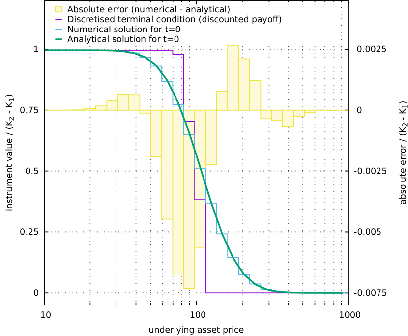
Figure 1: Corridor valuation. Comparison of a numerical solution obtained with MPDATA with the corresponding analytical solution (i.e., the Black-Scholes formula). Instrument parameters: a sold option with strike $K_{1}=75$ and a bought option with strike $K_{2}=125$, 6-month tenure (time to expiry), risk-free rate $r=0.8\%$, volatility $\sigma=0.6$.

The numerical solution was obtained with the following settings of libmpdata++ (consult [20] for details): one corrective iteration, non-oscillatory, infinite-gauge, and divergent-flow options enabled, a choice for which the highest convergence rate in time was observed. Figure 1 qualitatively depicts the match between the numerical and analytical solutions. It shows that the error is smallest near the domain boundaries, confirming that the domain extent is sufficient for the given parameters. The solution does not feature values below zero (the minimum of the initial condition), which illustrates the positive definiteness of MPDATA. The solution does not feature values above the maximum of the initial condition which in turn demonstrates the conservativeness and monotonicity (non-oscillatory character) of the scheme.

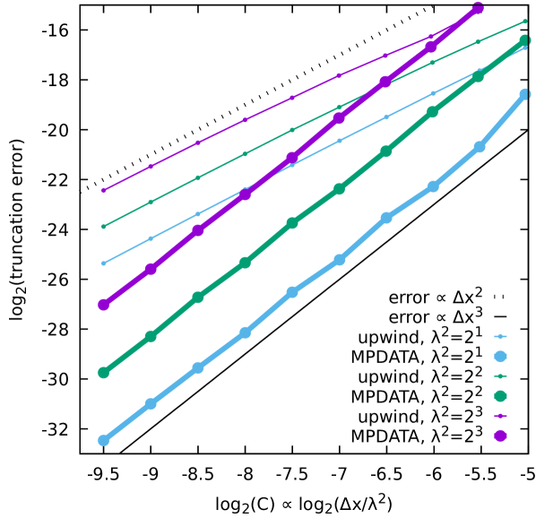
Figure 2: Solution accuracy in terms of the spatial discretisation. Truncation error as a function of the Courant number $C=u\frac{\Delta t}{\Delta x}$ which, for fixed $\lambda^{2}$, is proportional to the gridstep. Thin lines correspond to the basic upwind scheme (first iteration of MPDATA only), thick lines correspond to results obtained with one corrective iteration of MPDATA. Three datasets plotted for three different values of $\lambda^{2}$. The dotted and solid black lines depict the slopes corresponding to first-order and second-order convergence.

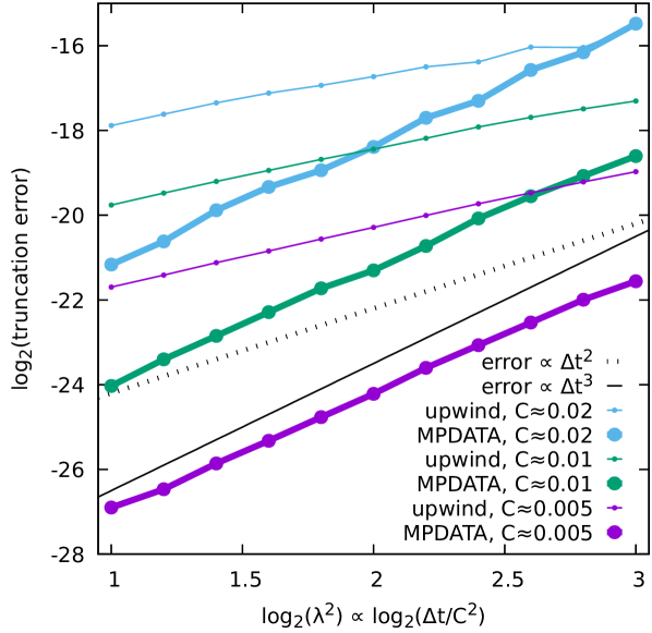
Figure 3: Solution accuracy in terms of the temporal discretisation. Truncation error as a function of the $\lambda^{2}$ parameter which, for fixed $C$, is proportional to the timestep. Three datasets plotted for three different values of $C$ (values given approximately as the solution procedure adjusts the requested value so that the number of timesteps is an integer). Other plot elements are as in Fig. 2.

A quantitative analysis of the errors arising from the numerical integration is summarised in Figs 2-3. The accuracy of the solution is quantified using an $L_{2}$ measure of the average error per timestep and per gridstep, defined following [2] as:

$$E=\sqrt{\left.\sum\limits_{i=1}^{n_{x}}\left[\psi_{n}(x_{i})-\psi_{a}(x_{i})\right]^{2}/(n_{x}\cdot n_{t})\right|_{t=0}}$$ (19)

where $\psi_{n}$ is the numerical solution, and $\psi_{a}$ is the analytical one given by eq. (17). In Fig. 2, the base-2 logarithm of $E$ is plotted against the base-2 logarithm of $C=u\frac{\Delta t}{\Delta x}$ for several settings of $\lambda^{2}$. Thick lines represent solutions obtained with two iterations (labelled as MPDATA), thin lines represent solutions obtained with a single-pass scheme, i.e., the basic upwind algorithm. All other solution parameters were set as in the example depicted in Fig. 1.

Since, for a given value of $\lambda^{2}$, $C$ is proportional to the gridstep $\Delta x$, the slopes of the plotted curves depict how the results converge when refining the spatial discretisation. To facilitate interpretation, two additional curves were plotted, depicting the theoretical slopes for first-order and second-order accuracy. Figure 2 confirms that for the problem at hand, and for the three presented settings of $\lambda^{2}$, MPDATA is of second-order accuracy in space, improving over the close to first-order accurate solutions obtained with the upwind scheme.

The rate of convergence of the numerical solution to the analytical one as a function of the timestep is depicted in Fig. 3, constructed similarly to Fig. 2, with base-2 logarithm of $\lambda^{2}$ on the abcissa. Since for a given value of $C$, $\lambda^{2}$ is proportional to the timestep $\Delta t$, the plotted curves depict the order of accuracy in time. In all presented cases, the MPDATA solutions are of second-order accuracy in time, while the convergence rate of the upwind solutions in time is below first order.

Summary and prospects

This work was intended to serve as a springboard for applications of MPDATA in quantitative finance. In this domain, the MPDATA family of numerical schemes appears to be particularly promising and adaptable for solving PDEs arising in derivative pricing problems. It possesses particularly appealing properties in terms of:

• positive definiteness (non-negativity of option price solutions by design),

• monotonicity (no spurious oscillations in the solutions),

• conservativeness and high-order accuracy (second-order in time and space for the basic MPDATA),

• multidimensionality (superior to dimensionally-split schemes; applicable to problems giving rise to multi-dimensional PDEs),

• robustness (explicit and hence trouble-free to implement, and apt to parallelisation via domain decomposition).

The prospects for the use of the MPDATA framework in quantitative finance lie in its applications in more sophisticated contexts. We describe in the Appendix, for instance, an extension of the developed framework to handle valuation of American options, for which finite difference methods are applied in the industry. Other potential applications include problems modelled with multi-dimensional PDEs such as in stochastic volatility models and in pricing derivatives incorporating dependence on the history of underlying processes (i.e., path-dependent derivatives, e.g., so-called Asian options), and in pricing of other multi-factor (e.g., multi-asset) derivatives.

Appendix A American option valuation using MPDATA

Problem formulation

American options differ from the European ones only by allowing the holder to exercise at any time prior to expiry. Pricing of American options leads to a free boundary problem since there is a boundary, not known in advance, that for any time $t$ separates the regions where it is either optimal to continue holding the option or optimal to exercise it immediately [see e.g. 13, Sec. 12.3]. Under the herein embraced assumptions, notably without considering the so-called costs of carry [13, sec. 5.10], the boundary is unique (for a discussion of the more general setting, in which the boundary can bifurcate, see [28]). In deriving eq. (4), it was mentioned that the riskless portfolio $\Pi$ must evolve according to the risk-free interest rate $r$. This is because, over the lifetime of the option, if the portfolio had a rate of return less than $r$, an investor holding the portfolio would sell it for $\Pi$, invest $\Pi$ at the rate $r$, and buy the portfolio back at a later stage, making riskless profit. If the rate of return is greater than $r$, an investor would borrow $\Pi$ to buy the portfolio, and then sell it at a later time, paying back the debt and making riskless profit. The difference in the case of American options is that the latter case does not hold: in the intervening time between buying the portfolio and selling it, the investor runs the risk that the sold option would be exercised against them at any moment, changing the rate of return of the portfolio. This implies that the price process $f$ for American options only satisfies

$$-\Big{(}\frac{\partial f}{\partial t}+rS\frac{\partial f}{\partial S}+\frac{\sigma^{2}}{2}S^{2}\frac{\partial^{2}f}{\partial S^{2}}-rf\Big{)}\geq 0$$ (20)

On the other hand, at any time $t$, $f(S,t)\geq P(S,t)$, where $P(S,t)$ is the payoff function of the option if it is exercised at time $t$. This is because of the no-arbitrage condition: if $f(S,t)<P(S,t)$, the holder of the option would exercise immediately, collect the payoff, and then use it to buy the option back at $f(S,t)$. Thus, for a standard put option with strike $K$,

$$f(S,t)-(K-S)\geq 0$$ (21)

When $f(S,t)=P(S,t)$, the option holder must exercise immediately - continuing to hold the option puts the holder at risk of loss. Replacement in eq. (20) shows that strict inequality holds in such case. On the other hand, when $f(S,t)>P(S,t)$, the holder of the option should continue to hold it, and in this case, equality holds in eq. (20). This, together with the terminal condition

$$f(S,T)=\max(K-S,0)$$ (22)

describes a so-called linear complementarity problem, where strict inequality holds in at most one of eq.s (20) and (21).

Numerical solution procedure

A simple (non-second-order) yet robust way to represent the linear complementarity problem in the numerical framework embraced herein is to supplement the solved transport equation with a source term representing the linear complementarity problem, and to integrate according to the following recipe:

$$\psi^{*}=\text{MPDATA}(\psi^{n})$$ (23)

$$R^{n}=\frac{\max\left(\psi^{*},f(S,T)\exp(-rt^{n+1})\right)-\psi^{*}}{\Delta t}$$ (24)

$$\psi^{n+1}=\psi^{*}+\Delta tR^{n}$$ (25)

The source term $R$ effectively represents a limiter on the time derivative of $\psi$ (and hence, the time derivative of $f$). For a recent discussion of the formulation of the free boundary problem in terms of a linear complementarity constraint on the time derivative of $f$, as opposed to $f$ itself, see [29].

To note, an upwind-based numerical solution for the American option valuation problem was previously studied in [30]. That study, however, did not involve the transformation of the Black-Scholes equation into a constant-coefficient advection-diffusion equation.

Results

We corroborate the numerical integration results for American put option prices against the estimates obtained from the approximate analytical formula derived in [31]. The payoff function for the put option is given by eq. (22). A log-linear extrapolation for both $\psi$ and its derivative is used for the boundary condition in this case. The grid is chosen to include the point corresponding to the spot price $x=\ln(S_{0})$.

Results of a series of integrations carried out for different option tenures $T$ and spot prices $S_{0}$, and with three settings for the Courant number $C=u\frac{\Delta x}{\Delta t}$, are given in Table 1. All simulations were carried out with $\lambda^{2}=2$, $\sigma=0.2$, $r=0.08$ and $K=100$, on a grid covering the range of $S\in(0.05,500)$. The obtained option valuations converge with decreasing $C\sim\Delta x/\lambda^{2}$ to the prices obtained with the Bjerksund and Stensland formula (column labelled BS93). The error measures computed following eq. (19), and given in the columns labelled $\log_{2}(E)$, depict a convergence rate in $\Delta x$ not less than first order. Results obtained with the upwind scheme (not shown) are characterised by larger errors than with MPDATA, but comparable convergence rate, illustrating that the convergence rate is constrained by the treatment of the linear-complementarity condition. For reference, prices of European put options with the same parameters, obtained with the analytical Black-Scholes formula (18), are given in the last column.

Table 1: Prices of American options obtained numerically compared with the Bjerksund and Stensland analytical formula (BS93), and with the prices of corresponding European options. Notation: $T$ – option tenure, $S_{0}$ – spot price, $C$ – Courant number, $E$ – error measure, $f(S_{0},0)$ – option price.

		C$\approx$0.02	C$\approx$0.01	C$\approx$0.005
$T$	$S_{0}$	$\log_{2}(E)$	$\log_{2}(E)$	$\log_{2}(E)$	$f(S_{0},0)$	BS93	European
0.25	80	-8.3	-10.1	-11.3	19.997	20.000	18.089
	90	-8.1	-10.0	-11.3	10.036	10.011	9.045
	100	-8.0	-10.0	-11.3	3.229	3.162	3.037
	110	-8.3	-10.0	-11.3	0.668	0.649	0.640
	120	-8.2	-10.2	-11.3	0.090	0.087	0.086
0.50	80	-8.7	-10.2	-11.4	20.000	20.000	16.648
	90	-8.5	-10.2	-11.4	10.290	10.240	8.834
	100	-8.5	-10.2	-11.3	4.193	4.109	3.785
	110	-8.7	-10.2	-11.4	1.413	1.372	1.312
	120	-8.6	-10.3	-11.4	0.399	0.385	0.376
3.00	80	-9.4	-11.4	-13.1	19.998	20.000	10.253
	90	-9.3	-11.4	-13.0	11.697	11.668	6.783
	100	-9.3	-11.4	-13.0	6.932	6.896	4.406
	110	-9.5	-11.4	-13.1	4.155	4.118	2.826
	120	-9.3	-11.4	-13.1	2.510	2.478	1.797

References

References

- [1] P. Smolarkiewicz, A simple positive definite advection scheme with small implicit diffusion, Mon. Weather Rev. 111 (1983) 479–486. doi:10.1175/1520-0493(1983)111<0479:ASPDAS>2.0.CO;2.
- [2] P. Smolarkiewicz, A fully multidimensional positive definite advection transport algorithm with small implicit diffusion, J. Comp. Phys. 54 (1984) 325–362. doi:10.1016/0021-9991(84)90121-9.
- [3] P. Smolarkiewicz, L. Margolin, MPDATA: A finite-difference solver for geophysical flows, J. Comp. Phys. 140 (1998) 459–480. doi:10.1006/jcph.1998.5901.
- [4] P. Smolarkiewicz, Multidimensional positive definite advection transport algorithm: an overview, Int. J. Num. Meth. Fluids 50 (2006) 1123–1144. doi:10.1002/fld.1071.
- [5] P. Smolarkiewicz, J. Szmelter, F. Xiao, Simulation of all-scale atmospheric dynamics on unstructured meshes, J. Comp. Phys. 322 (2016) 267–287. doi:10.1016/j.jcp.2016.06.048.
- [6] F. Black, M. Scholes, The pricing of options and corporate liabilities, J. Polit. Economy 81 (3) (1973) 637–654. doi:10.1086/260062.
- [7] D. Duffy, Finite Difference Methods in Financial Engineering- A Partial Differential Equation Approach, Wiley, 2006.
- [8] D. Duffy, A critique of the Crank-Nicolson scheme, strengths and weaknesses for financial instrument pricing, WILMOTT magazine 4 (2004) 68–76. doi:10.1002/wilm.42820040417.
- [9] M. Osborne, Brownian motion in the stock market, Operations Research 7 (1959) 145–173. doi:10.1287/opre.7.2.145.
- [10] L. Bachelier, Théorie de la spéculation, Ann. Sci. École Norm. Sup. 3 (1900) 21–86.
- [11] W. Schachermayer, J. Teichmann, How close are the option pricing formulas of bachelier and Black-Merton-Scholes?, Math. Finance. 18 (2007) 155–170. doi:10.1111/j.1467-9965.2007.00326.x.
- [12] W. Paul, J. Baschnagel, Stochastic Processes: From Physics to Finance, 2nd Edition, Springer, 2013. doi:10.1007/978-3-319-00327-6.
- [13] M. Joshi, The Concepts and Practice of Mathematical Finance, 2nd Edition, Cambridge, 2008.
- [14] K. Morton, Numerical Solution of Convection-Diffusion Problems, Chapman and Hall, London, 1996.
- [15] P. Smolarkiewicz, T. Clark, The multidimensional positive definite advection transport algorithm: Further development and applications, J. Comp. Phys. 67 (1986) 396–438. doi:10.1016/0021-9991(86)90270-6.
- [16] E. Sousa, Insights on a sign-preserving numerical method for the advection–diffusion equation, Int. J. Num. Meth. Fluids 61 (2009) 864–887. doi:10.1002/fld.1984.
- [17] P. Smolarkiewicz, J. Szmelter, MPDATA: An edge-based unstructured-grid formulation, J. Comp. Phys. 206 (2005) 624–649. doi:10.1016/j.jcp.2004.12.021.
- [18] E. Cristiani, Blending Brownian motion and heat equation, J. Coupled Syst. Multiscale Dyn. 3 (2015) 351–356. doi:10.1166/jcsmd.2015.1089.
- [19] L. Bauer, The relation between “potential temperature” and “entropy”, Phys. Rev. (Series I) 26 (1908) 177–183. doi:10.1103/PhysRevSeriesI.26.177.
- [20] A. Jaruga, S. Arabas, D. Jarecka, H. Pawlowska, P. K. Smolarkiewicz, M. Waruszewski, libmpdata++ 1.0: A library of parallel MPDATA solvers for systems of generalised transport equations, Geosci. Model Dev. 8 (4) (2015) 1005–1032. doi:10.5194/gmd-8-1005-2015.
- [21] B. Leonard, A survey of finite differences of opinion on numerical muddling of the incomprehensible defective confusion equation, in: T. Hughes (Ed.), Finite Element Methods for Convection Dominated Flows, ASME, 1979, pp. 1–17.
- [22] M. Waruszewski, C. Kühnlein, H. Pawlowska, P. Smolarkiewicz, MPDATA: Third-order accuracy for variable flows, J. Comp. Phys. 359 (2018) 361–379. doi:10.1016/j.jcp.2018.01.005.
- [23] R. Zvan, P. Forsyth, K. Vetzal, Robust numerical methods for pde models of asian options, J. Comp. Finance, 1 (1998) 39–78. doi:10.1.1.34.1853.
- [24] Y.-K. Kwok, K.-W. Lau, Accuracy and reliability considerations of option pricing algorithms, J. Futures Markets 21 (10) (2001) 875–903. doi:10.1002/fut.2001.
- [25] R. Geske, K. Shastri, Valuation by approximation: A comparison of alternative option valuation techniques, J. Fin. Quant. Analysis 20 (1) (1985) 45–71. doi:10.2307/2330677.
- [26] J. Hull, A. White, Valuing derivative securities using the explicit finite difference method, J. Fin. Quant. Analysis 25 (1) (1990) 87–99. doi:10.2307/2330889.
- [27] W. Hogarth, B. Noye, J. Stagnitti, J. Parlange, G. Bolt, A comparative study of finite difference methods for solving the one-dimensional transport equation with an initial-boundary value discontinuity, Comp. Math. Applic. 20 (1990) 67–82. doi:10.1016/0898-1221(90)90220-E.
- [28] A. Battauz, M. De Donno, A. Sbuelz, Real options and American derivatives: The double continuation region, Manag. Sci. 61 (2015) 1094–1107. doi:10.1287/mnsc.2013.1891.
- [29] O. Bokanowski, K. Debrabant, High order finite difference schemes for some nonlinear diffusion equations with an obstacle term (2018). arXiv:1802.05681.
- [30] C. Vázquez, An upwind numerical approach for an American and European option pricing model, Appl. Math. Comp. 97 (1998) 273–286. doi:10.1016/S0096-3003(97)10122-9.
- [31] P. Bjerksund, G. Stensland, Closed-form approximation of American options, Scand. J. Manag. 9 (1993) 87–99. doi:10.1016/0956-5221(93)90009-H.