Optimal counter-current exchange networks

Abstract

We present a general analysis of exchange devices linking their efficiency to the geometry of the exchange surface and supply network. For certain parameter ranges, we show that the optimal exchanger consists of densely packed pipes which can span a thin sheet of large area (an ‘active layer’), which may be crumpled into a fractal surface and supplied with a fractal network of pipes. We derive the efficiencies of such exchangers, showing the potential for significant gains compared to regular exchangers (where the active layer is flat), using parameters relevant for biological systems.

I Introduction

The design of efficient exchange devices is an important problem in engineering and biology. A wide variety of heat exchangers, such as plate, coil and counter-current, are employed in industrial settings Perry , while in nature, leaf venation, blood circulation networks, gills and lungs have evolved to meet multiple physiological imperatives. A distinctive feature of the biological examples is their complex, hierarchical (fractal) nature West , with branching and usually anastomosing geometries Katifori ; Makanya . It is clear that one reason for this is the possibility to include a large surface for exchange within a compact volume, as in the human lungs, which comprise an alveolar area greater than $50{\rm m}^{2}$ Wiebe . However, maximal surface area is unlikely to be the only criterion for optimization. As an example, West et al have analyzed biological circulatory systems on the basis that power is minimized with the constraint that a minimum flux of respiratory fluid is brought to every cell in the volume of an organism, and were able to explain well known allometric scaling laws in biology West .

Although scaling behaviors are known in some cases, the detailed geometry of optimal exchangers remains elusive. With the advance of new fabrication technologies such as 3D printing Hague , it is becoming possible to build structures of comparable complexity to biological systems, so there is a need not only to understand the principles and compromises upon which natural systems are based, but also for that understanding to be constructive, mapping system parameters to actual designs.

The analytic literature in this area has focused on heat transfer from a fluid to a solid body, with a particular emphasis on cooling of integrated circuits Tuckerman . Branching fractal networks are much studied due to their ability to give good heat transfer with a low pressure drop Bejan ; Chen (although sometimes simpler geometries can be more efficient Escher ), and multiscale structures are also found to have a high heat transfer density Fautrelle .

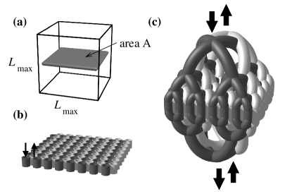
Figure 1: (a) Schematic of the geometry of a counter-current heat exchanger ‘active layer’ fitting inside a prescribed cubic volume of side length $L_{\max}$. (b) Detail of the active layer, showing a regular array of pipes carrying alternately counter-flowing streams. (c) The active layer connected to a branching and (on the other side) anastomosing fractal supply network.

In this contribution, we consider exchange as a general process, which includes gas, solute and heat exchange, and we look for the optimal designs which can ensure complete exchange (to be defined below) while requiring a minimum amount of mechanical power to generate the necessary fluid flows.

We use the language of thermal processes, since the relevant material properties have widely used notation. However, with a suitable translation of quantities, the analysis also applies to mass transfer. For example, in a thermal system with linear materials, the quantities: temperature, heat, heat capacity per unit volume and thermal conductivity would correspond in a system of gas exchange to: partial pressure of gas, mass of gas, Henry’s law coefficient and the product of the Henry’s law coefficient and gas diffusivity. For mass exchange with solutes, the analogue of temperature would be osmotic pressure of the solute.

II Non-dimensionalization

The first step is to gather problem parameters into dimensionless groups, which span the space of possible exchange problems.

Suppose there are two counter-flowing (perhaps dissimilar) fluids with given properties: thermal conductivities $\kappa_{j}$ ($j\in\{1,2\}$), heat capacities per unit volume $C_{j}$ and viscosities $\eta_{j}$. Let there be an imposed difference $\Delta T$ in the inlet temperatures, and an imposed volumetric flow rate $Q_{1}$ of fluid 1 (while we are free to choose $Q_{2}$). For example, if we are considering thermoelectric generation from the exhaust gases of a vehicle, $Q_{1}$ would be the volumetric flow of exhaust gases. Analogously, in gas exchange for vertebrate respiration, we take the required blood flow to the lungs or gills as the fixed quantity $Q_{1}$.

The fluid streams between which exchange occurs are assumed separated by walls of thickness $w$ (taken to be the minimum consistent with biological or engineering constraints) and thermal conductivity $\kappa_{\rm wall}$; the latter again an imposed constraint. We assume that the exchanger needs to be compact, in that it fits inside a roughly cubical volume of side length $L_{\rm max}$, and the pipes, being straight, are each of length $L\leq L_{\max}$. Last, we wish the exchange process to go to completion, in that the total exchanged power is of order $E_{\rm end}=C_{1}Q_{1}\Delta T$, which results in the outlet temperature of flow 1 being equal to the inlet temperature of flow 2, and conversely. Our aim is to find an exchange network which satisfies all these constraints (which we believe are a typical set for both engineering and biological systems), while requiring the minimum amount of power to drive the flow through the network.

To proceed, we non-dimensionalize on $L_{\max}$ and $\kappa_{\rm wall}$, defining the new quantities:

$$\hat{w}\equiv w/L_{\max},\ \ \ \hat{r}_{j}\equiv r_{j}/L_{\rm max},\ \ \ \hat{L}\equiv L/L_{\max},$$

$$\hat{A}\equiv A/L_{\max}^{2}\ \ \ {\rm and}\ \ \ \hat{\kappa}_{j}\equiv\kappa_{j}/\kappa_{\rm wall}.$$

The specification of the problem can be conveniently reduced to three non-dimensional parameters, the first two of which capture the asymmetry of the two fluids:

$$\beta\equiv(C_{1}/C_{2})^{2}(\eta_{2}/\eta_{1})\ \ \ {\rm and}\ \ \ \gamma\equiv\kappa_{1}/\kappa_{2}.$$ (1)

We then note that if all the available volume were filled with pipes of the smallest possible radius, and the two fluids were set to uniform temperatures differing by $\Delta T$, then there would be a maximum possible exchanged power of order $E_{\rm max}=\Delta T\kappa_{\rm wall}L_{\rm max}^{3}/w^{2}$. Thus our last parameter is the ratio of the required exchange rate to this maximum:

$$\epsilon\equiv E_{\rm end}/E_{\rm max}=Q_{1}C_{1}w^{2}/(L_{\max}^{3}\kappa_{\rm wall}),$$ (2)

and we typically expect $\epsilon\ll 1$.

III Optimal regular exchangers

We consider a regular array of counter-flowing streams in $N_{j}$ straight pipes of radii $r_{j}$ ($j=1,2$) and length $L$ (the same for both types), where we initially ignore any feed network to supply the individual pipes. This regular array is shown in figure 1(b), and we describe this array of pipes as the ‘active layer’, since it is where exchange actually occurs.

To proceed, we make three geometric approximations: First, assuming roughly circular pipes, we approximate the total cross section (perpendicular to flow) of the array as

$$A\approx\pi N_{1}(r_{1}+w/2)^{2}+\pi N_{2}(r_{2}+w/2)^{2}.$$ (3)

Second, let $\alpha$ be the area across which exchange occurs, then if no clustering of one type occurs $\alpha$ will be approximately the minimum of the two pipe perimeters, multiplied by $L$. We thus propose a simple approximation to the total area across which exchange occurs:

$$\alpha\approx\left[(N_{1}2\pi r_{1}L)^{-1}+(N_{2}2\pi r_{2}L)^{-1}\right]^{-1}.$$ (4)

Third, we approximate the thermal conductance per unit area across which exchange occurs to be

$$s\approx\left[(w/\kappa_{\rm wall})+(r_{1}/\kappa_{1})+(r_{2}/\kappa_{2})\right]^{-1}.$$ (5)

When is exchange complete? We assume the pipes are slender, so that heat diffusion along the length of a pipe is negligible compared to across its width (and also to advective transport along its length); and that the temperature over a cross section perpendicular to its length is roughly uniform. Let $z$ be the distance along a pipe, with $z=0$ being the upstream end of fluid 1 and the downstream end of fluid 2, so the average temperatures over cross sections of each of the two types of pipe are $T_{j}(z)$. We define the difference of inlet temperatures to be $\Delta T\equiv T_{1}(0)-T_{2}(L)$. By considering the total heat flux per unit length $J(z)$ between the two sets of pipes, we can write down the material derivative of temperature as each fluid moves along its respective pipe:

$$\pi N_{j}r_{j}^{2}C_{j}\frac{DT_{j}}{Dt}=(-)^{j}J(z),$$ (6)

where, since the average flow speed in the pipes of type $j\in\{1,2\}$ is $Q_{j}/(N_{j}\pi r_{j}^{2})$, the material derivative is

$$\frac{D}{Dt}\equiv\frac{\partial}{\partial t}+(-)^{j+1}\frac{Q_{j}}{N_{j}\pi r_{j}^{2}}\frac{\partial}{\partial z}.$$ (7)

If $s$ is the thermal conductance per unit area between pipes we note:

$$J(z)\approx\alpha s[T_{1}(z)-T_{2}(z)]/L.$$ (8)

In the steady state regime, $\partial/\partial t\equiv 0$ so Eqs. (6) lead to an exchanged power $E$ given by

$$\frac{E}{s\alpha\Delta T} = \frac{\xi_{1}\xi_{2}(e^{1/\xi_{1}}-e^{1/\xi_{2}})}{\xi_{2}e^{1/\xi_{1}}-\xi_{1}e^{1/\xi_{2}}}\approx\min(1,\xi_{1},\xi_{2})$$ (9)

$$\xi_{j} \equiv Q_{j}C_{j}/(\alpha s).$$ (10)

Complete exchange means $E\approx C_{1}Q_{1}\Delta T$, which from Eq. (9) is equivalent to $\xi_{1}\leq\xi_{2}$ and $\xi_{1}\leq 1$. We note from the analysis accompanying Eq. (9) that there is a special case of a ‘balanced’ exchanger, in which $Q_{1}C_{1}=Q_{2}C_{2}$ (so $\xi_{1}=\xi_{2}$) and the change of temperature with $z$ for both streams is linear, rather than being exponential. The optimal exchanger should have this property, since otherwise some of the pipe length will contribute to dissipated power but not exchange. Thus $Q_{2}$ is determined by the imposed value of $Q_{1}$.

System:	T.E.G.	Pigeon	Salmon
Exchanged:	Heat	Oxygen	Oxygen
$L_{\max}/{\rm m}$	$2.0\ 10^{-1}$	$5.0\ 10^{-2}$	$2.0\ 10^{-2}$
$w$/m	$5.0\ 10^{-4}$	$5.0\ 10^{-7}$	$5.0\ 10^{-7}$
$Q_{1}/$m3s-1	$5.0\ 10^{-2}$	$2.0\ 10^{-5}$	$1.0\ 10^{-6}$
$C_{1}$/S.I.	$1.0\ 10^{3}$	$2.0\ 10^{-6}$	$2.0\ 10^{-6}$
$C_{2}$/S.I.	$1.0\ 10^{3}$	$1.3\ 10^{-5}$	$1.0\ 10^{-7}$
$\kappa_{1}$/S.I.	$4.0\ 10^{-2}$	$1.8\ 10^{-16}$	$1.6\ 10^{-16}$
$\kappa_{2}$/S.I.	$4.0\ 10^{-2}$	$2.3\ 10^{-10}$	$1.6\ 10^{-16}$
$\kappa_{\rm wall}$/S.I.	$1.0\ 10^{1}$	$1.8\ 10^{-16}$	$1.6\ 10^{-16}$
$\eta_{1}$/Pa s	$4.0\ 10^{-5}$	$4.0\ 10^{-3}$	$4.0\ 10^{-3}$
$\eta_{2}$/Pa s	$4.0\ 10^{-5}$	$4.0\ 10^{-5}$	$1.0\ 10^{-3}$
$\beta$	$1.0\ 10^{0}$	$2.4\ 10^{-4}$	$1.0\ 10^{2}$
$\gamma$	$1.0\ 10^{0}$	$7.8\ 10^{-7}$	$1.0\ 10^{0}$
$\epsilon$	$1.6\ 10^{-4}$	$4.4\ 10^{-4}$	$3.9\ 10^{-4}$
$r_{1,\rm reg}$/m	$1.0\ 10^{-3}$	$2.5\ 10^{-5}$	$5.2\ 10^{-6}$
$r_{2,\rm reg}$/m	$1.0\ 10^{-3}$	$2.2\ 10^{-6}$	$2.1\ 10^{-5}$
$A_{\rm reg}$/m2	$4.0\ 10^{-2}$	$2.5\ 10^{-3}$	$4.0\ 10^{-4}$
$L_{\rm reg}$/m	$2.0\ 10^{-1}$	$5.0\ 10^{-2}$	$2.0\ 10^{-2}$
$P_{\rm reg}$/W	$2.4\ 10^{1}$	$6.2\ 10^{-1}$	$7.7\ 10^{-1}$
$r_{1,\rm frac}$/m	$5.1\ 10^{-4}$	$5.0\ 10^{-6}$	$5.0\ 10^{-6}$
$r_{2,\rm frac}$/m	$5.1\ 10^{-4}$	$5.4\ 10^{-7}$	$7.3\ 10^{-6}$
$A_{\rm frac}$/m2	$6.6\ 10^{-2}$	$1.0\ 10^{-2}$	$7.6\ 10^{-4}$
$L_{\rm frac}$/m	$4.3\ 10^{-2}$	$7.1\ 10^{-4}$	$2.9\ 10^{-3}$
$P_{\rm frac}$/W	$1.8\ 10^{1}$	$6.0\ 10^{-2}$	$4.0\ 10^{-1}$

Table 1: Estimated parameters for various real systems. ‘S.I.’ refers to the international system of units; so for thermal systems $C$ will have units ${\rm Jm}^{-3}{\rm K}^{-1}$ and $\kappa$ will have units ${\rm Wm}^{-1}{\rm K}^{-1}$. For gas exchange, $C$ will have units kilogram of relevant gas per m³ of fluid, per Pascal of partial pressure, and $\kappa$ will have units ${\rm kg\,s}^{-1}{\rm m}^{-1}{\rm Pa}^{-1}$ (so that $\kappa/C$ is a diffusivity). ‘T.E.G.’ is thermo-electric generation from internal combustion engine exhaust (we have chosen values corresponding to a car/personal automobile). For the animal respiratory systems we assume that transport across the exchange membrane is similar to that of water. For blood, we assume that oxygen can exist in a mobile form (dissolved in the water-like serum) and an immobile form (bound to haemoglobin). Thus the oxygen ‘conductivity’ $\kappa_{1}$ for blood is the same as for water, while $C_{1}$ is increased over that of water by the carrying capacity of haem. Data are from Refs. CRC ; Cussler ; Schmidt ; Butler ; Kicenuik . Results for a regular exchange network are indicated by the subscript ‘reg’; while the results for the fractal exchange surfaces (denoted by a subcript ‘frac’) use a Hausdorff dimension $d=2.33$. For the cases of pigeon and salmon respiration, we impose the additional constraint that $r_{1}>5\mu\rm m$, in order to allow erythrocytes to pass through blood vessels (type 1 pipes). This appears to only affect the fractal case, and without this requirement, the optimized value of $r_{1}$ for this fractal case would be $1.5\mu\rm m$ and $0.4\mu\rm m$ for pigeon and salmon respectively.

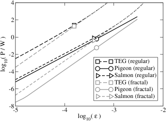
Figure 2: Plots of power dissipated in exchange for the three cases of table 1. Here we change $Q_{1}$ to achieve different values of $\epsilon$. The actual cases in table 1 are shown as symbols. For the cases of ‘pigeon’ and ‘salmon’, we additionally impose the constraint that blood vessels (type 1 pipes) should be large enough to carry erythrocytes (taken as the condition $r_{1}>5\mu\rm m$).

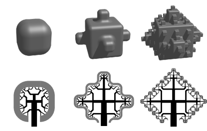
Figure 3: Top row: schematic of the active layer of figure 1(a), corrugated into a hierarchical (fractal) surface, comprising (left to right) greater area and more iterations of the fractal. Bottom row: Schematic section through these surfaces showing the fractal supply network in the interior (the corresponding network outside is not shown, and will require a more complex design to ensure equal flow to all parts of the active layer).

Now we seek to minimize the total power $P$ required to run the exchanger, $P=Q_{1}\Delta p_{1}+Q_{2}\Delta p_{2}$, where $\Delta p_{j}$ are the pressures dropped across the two types of pipes. For laminar (Poiseuille) flow, and using the ‘balanced’ condition $Q_{1}C_{1}=Q_{2}C_{2}$ to eliminate $Q_{2}$, we obtain:

$$P = P_{0}\epsilon^{2}\hat{L}\left(\frac{1}{N_{1}\hat{r}_{1}^{4}}+\frac{\beta}{N_{2}\hat{r}_{2}^{4}}\right),$$ (11)

$$P_{0} \equiv 8\eta_{1}\kappa_{\rm wall}^{2}L_{\max}^{3}/(\pi w^{4}C_{1}^{2}).$$ (12)

Our task is to minimize the power $P$ to drive the flow in Eq. (11) by choosing the five quantities $N_{j}$, $\hat{r}_{j}$ and $\hat{L}$, while ensuring the exchanger is compact (fits in the required volume):

$$\max(\hat{r}_{j})\leq\hat{L}\leq 1,$$ (13)

$$\hat{A}=\pi N_{1}(\hat{r}_{1}+\hat{w}/2)^{2}+\pi N_{2}(\hat{r}_{2}+\hat{w}/2)^{2}\leq 1,$$ (14)

and also that exchange is complete, which from $\xi_{1}\leq 1$ and Eqs. (4), (5), (10) leads to

$$\frac{\epsilon}{\hat{w}^{2}2\pi\hat{L}}\left(\frac{1}{N_{1}\hat{r}_{1}}+\frac{1}{N_{2}\hat{r}_{2}}\right)\left(\hat{w}+\frac{\hat{r}_{1}}{\hat{\kappa}_{1}}+\frac{\hat{r}_{2}}{\hat{\kappa}_{2}}\right)\leq 1.$$ (15)

The optimization can then be performed numerically with the constraints (13), (14) and (15). We do this in two different ways, which give essentially identical results: we either repeatedly choose a random direction in the five dimensional space of $(N_{j},\hat{r}_{j},\hat{L})$ and follow this direction until either the dissipated power does not fall or a constraint is encountered; or, we impose completeness of exchange in Eq. (15) as an equality, which allows us to determine $\hat{L}$ given the other variables, and then perform an exhaustive search for the minimum power over the more tractable 4-dimensional space $(N_{j},\hat{r}_{j})$.

Table 1 shows the geometry of some optimized regular exchangers for real cases, and the optimized results are included in figure 2 with the label ‘regular’.

IV Scaling of regular exchangers and limiting conditions

It is interesting to look at what limits the exchanger efficiency in different cases. For the examples studied here, the numerical results show that over essentially the entire range of $\epsilon$, Eqs. (14) and, unsurprisingly, (15) are satisfied as equalities. Furthermore, $\hat{w}$ is typically much less than $\hat{r}_{j}$ or $\hat{r}_{j}/\hat{\kappa}_{j}$.

For symmetric exchangers, where $N_{1}=N$, $\hat{r}_{1}=\hat{r}_{2}$ and $\hat{\kappa}_{1}=\hat{\kappa}_{2}$, we can see the consequences of this for the scaling behavior with $\epsilon$, because Eqs. (14) and (15) reduce to

$$2\pi N_{1}\hat{r}_{1}^{2}\approx 1\ \ \ {\rm and}\ \ \ \frac{\epsilon}{\hat{w}^{2}2\pi\hat{L}}\cdot\frac{2}{N_{1}\hat{r}_{1}}\cdot\frac{\hat{2r}_{1}}{\hat{\kappa}_{1}}\approx 1,$$ (16)

which implies the dissipated power

$$P\approx 16\pi P_{0}\epsilon^{3}/(\hat{\kappa}_{1}\hat{w}^{2}).$$ (17)

Two observations follow from this rough analysis: First, the dissipated power in this approximation does not depend on $\hat{L}$, so that although the numerical results indicate that optimization pushes $\hat{L}$ towards unity, this is only a weakly selected result. Thus exchangers with very similar dissipated power can be made from rather thin active layers [as shown schematically in figure 1(b)] without incurring a strong penalty. This is useful in allowing room for the supply network that we will wish to attach to the active layer.

Second, an interesting question to ask for an optimal exchange network is: which constraint is significantly limiting the performance? The non-trivial constraint in this case is typically the area $\hat{A}$ of the active layer in Eq. (14), which we would prefer to make larger than $L_{\max}^{2}$.

Taken together, these observations imply that a route to further optimization is to have an active layer which is both thin and also folded in some way to accommodate a larger area inside the prescribed volume of the device; an approach we will pursue further in section VI below.

V The branched supply network

So far, we have considered the active layer of the exchanger as an independent entity. However, it must be supplied with the two working fluids, and for the optimization scheme above to be relevant, this supply network, which dissipates power but performs no significant exchange, should not dominate the power consumption of the whole device.

Consider therefore a branched (and fractal) supply network shown in figure 1(c), which brings the streams to the exchanger’s active layer. In contrast to Ref. West , we do not need the supply network to pass close to every point in space. Suppose that each pipe comprising the supply network branches into $b$ smaller pipes at each hierarchical level $k$ of the tree (where pipes with higher values of $k$ are smaller, and closer to the active layer where exchange occurs). Let the ratio of pipe radii between neighboring levels be $\rho<1$, and the ratio of pipe lengths be $\lambda$. The ratio of power dissipated between hierarchical levels is therefore

$$P_{k+1}/P_{k}=\lambda/(b\rho^{4}).$$ (18)

Since the active layer is densely covered with pipes, the condition to fit the supply network into space is $\rho\geq b^{-1/2}$. Therefore, provided $\lambda>b\rho^{4}$, the power will increase exponentially with $k$ and the overall power dissipation in the supply network will be of order that in the last layer; and therefore of the same order as in the active layer. The supply network will therefore not dominate the power dissipation.

VI Fractal exchange networks

From the solution above for optimum regular exchange networks, the lateral cross section $A$ always expands to its maximum value $L_{\max}^{2}$. If this restriction were lifted, a more efficient exchanger would likely be possible. This can be achieved by allowing the active layer (provided it is thin enough, and can still be provided with a branching supply network) to become corrugated, while still fitting within the prescribed roughly cubical volume $L_{\max}^{3}$ available. One way to do this is to turn the active layer into an approximation to a fractal surface. Thus suppose the active layer to corrugated into such a fractal surface over a range of lateral length scales down to a scale $x\geq L$ (where $L$ is the pipe length, and therefore the thickness of the layer). In the limit $x\rightarrow 0$ the surface would have some Hausdorff dimension Hausdorff , which we denote $d$. Figure 3 shows schematically an example in which the surface is the type I quadratic Koch surface with (in the limit) Hausdorff dimension $d_{\rm koch}=\ln 13/\ln 3\approx 2.33$. Let the area of the active layer be $A(x)$, where $A(L_{\rm max})=L_{\rm max}^{2}$, then from Hausdorff’s definition of dimension, we see that $A(x)=L_{\rm max}^{2}(x/L_{\rm max})^{2-d}$. We can therefore replace the inequality $\hat{A}\leq 1$ in Eq. (14) by

$$\hat{A}=\pi N_{1}(\hat{r}_{1}+\hat{w}/2)^{2}+\pi N_{2}(\hat{r}_{2}+\hat{w}/2)^{2}\leq\hat{L}^{2-d}.$$ (19)

Figure 2 shows the effect of $\epsilon$ (varied through altering $Q_{1}$) on the power dissipation for fractal exchangers corresponding to the scenarios in table 1, compared to that of the regular exchanger. Corrugating the exchange layer into a type I quadratic Koch surface leads to a significant reduction in the dissipated power for the two biological cases (factor gain of $10$ for pigeon lungs and $2$ for salmon gills). However, the small size of the optimum pipe radii $r_{1}$ may mean that this degree of optimization is precluded by other considerations. For instance, erythrocytes need to be able to pass through these type 1 (blood carrying) vessels.

Crumpling the active layer into a (limited length scale) fractal surface would also be expected to produce a novel scaling of dissipated power with $\epsilon$. The numerical results indicate that in the optimum exchanger $\hat{A}$ expands to its new maximum extent, so Eq. (19) is an equality. As above, Eq. (15) is an equality, but we find for the TEG case that $\hat{w}$ is comparable to $\hat{r}_{j}$, while $\hat{w}$ remains substantially less than $\hat{r}_{j}/\hat{\kappa}_{j}$. This leads in the symmetric case to the following versions of Eqs. (19) and (15):

$$\frac{9\pi}{4}N_{1}\hat{w}^{2}\approx\hat{L}^{2-d}\ \ \ {\rm and}\ \ \ \left(\frac{2\hat{r}_{1}}{\hat{\kappa}_{1}}\right)\left(\frac{2}{N_{1}\hat{r}_{1}}\right)\approx\frac{2\pi\hat{L}\hat{w}^{2}}{\epsilon},$$ (20)

(the first assuming for definiteness $\hat{w}\approx\hat{r}_{1}$), which implies the dissipated power is

$$P\approx\left(\frac{9}{2}\right)^{\frac{2}{3-d}}\frac{\pi P_{0}}{\hat{w}^{2}}\hat{\kappa}_{1}^{\frac{1-d}{3-d}}\epsilon^{\frac{5-d}{3-d}}.$$ (21)

For the quadratic Koch surface, this leads to $P\propto\epsilon^{4.01}$, which is close to the observed exponent in figure 2.

VII Conclusions

Exchange networks of the class we show here exhibit broadly power-law dependence of the dissipated power with the quantity $\epsilon$, which measures the required throughput: the rate of exchange of heat, gas or solute needed. This is true both for a fractally corrugated or a simple regular array of exchange pipes. However, the fractal exchangers demonstrate gains in efficiency when compared to regular exchangers for small values of $\epsilon$, and in particular for parameters relevant to biological systems. This is driven by the higher efficiency of a thin active exchange layer of large area; the fractal corrugations being one way to accommodate this geometry in a compact volume.

We note that the analysis we have performed here aims specifically to minimize required power while ensuring complete exchange has taken place and compactness of the exchange device. In practice, other design constraints may need to be included, for example a requirement that the network be robust Katifori or easily repairable Qu ; Farr under external attack Cohen2000 ; Cohen2001 ; or the cost of building the network may be significant compared to its operating costs Bohn ; Durand . Nevertheless, the conditions analyzed here are, we believe, relevant to a wide class of engineering and biological systems and could provide the basis for improved industrial efficiency and insights into the structures used for respiration in the living world.

References

- (1) Perry’s Chemical Engineers’ Handbook, Eighth Edition, D. W. Green and R. H. Perry, (McGraw-Hill, 2007).
- (2) G. West, J. H. Brown and B. J. Enquist, Science 276(5309), 122 (1997).
- (3) E. Katifori, G. J. Szöllösi and M. O. Magnasco, Phys. Rev. Lett. 104, 048704 (2010).
- (4) A. N. Makanya and V. Djonov, Microscopy Research and Technique 71(9), 689 (2008).
- (5) B.M. Wiebe and H. Laursen, Microscopy Research and Technique 32, 255 (1995).
- (6) R. Hague and P. Reeves, Ingenia, Issue 55, June (2013).
- (7) D.B. Tuckerman and R.F.W. Pease, Electron device letters 2(5), 126 (1981).
- (8) A. Bejan and M. R. Errera, Fractals 5(4), 685 (1997).
- (9) Y. Chen and P. Cheng, Int. J. Heat and Mass Transfer 45, 2643 (2002).
- (10) W. Escher, B. Michel and D. Poulikakos, Int. J. Heat and Mass Transfer 52(5-6), 1421 (2009).
- (11) A. Bejan and Y. Fautrelle, Acta Mechanica 163(1-2), 39 (2003).
- (12) M. V. Twigg, Applied Catalysis B: Environmental 70, 2 (2007).
- (13) Hagenbach, E. Ueber die Bestimmung der Zähigkeit einer Flüssigkeit durch den Ausfluss aus Röhren. Annalen der Physik und Chemie 109, 385-426 (1860).
- (14) D. R. Lide (Ed.), Handbook fo chemistry and physics, 75th Edn. (CRC Press, Inc., 1995).
- (15) E.L. Cussler Diffusion: Mass Transfer in Fluid Systems (2nd ed.). New York: Cambridge University Press (1997).
- (16) K. Schmidt-Nielsen, Animal physiology: adaptation and environment, Cambridge University Press, Cambridge (1990).
- (17) P.J. Butler, N.H. West and D.R. Jones, Journal of Experimental Biology 71, p7 (1977).
- (18) J.W. Kicenuik and D.R. Jones, Journal of Experimental Biology 69, p247 (1977).
- (19) F. Hausdorff, Mathematische Annalen 79(1–2), p157 (1919).
- (20) W. Quattrociocchi, G. Caldarelli and A. Scala, PLoS ONE 9(2), e87986 (2014).
- (21) R.S. Farr, J.L. Harer and T.M.A. Fink, Phys. Rev. Lett. 113(3), 138701 (2014).
- (22) R. Cohen, K. Erez, D. ben-Avraham and S. Havlin, Phys. Rev. Lett. 85, 4626 (2000).
- (23) R. Cohen, K. Erez, D. ben-Avraham and S. Havlin, Phys. Rev. Lett. 86, 3682 (2001).
- (24) S. Bohn and M. O. Magnasco, Phys. Rev. Lett. 98, 088702 (2007).
- (25) M. Durand, Phys. Rev. Lett. 98, 088701 (2007).