X-Rays Beware: The Deepest Chandra Catalogue of Point Sources in M31

Abstract

This study represents the most sensitive Chandra X-ray point source catalogue of M31. Using 133 publicly available Chandra ACIS-I/S observations totalling $\sim 1$ Ms, we detected 795 X-ray sources in the bulge, northeast, and southwest fields of M31, covering an area of $\approx$ 0.6 deg², to a limiting unabsorbed $0.5-8.0$ keV luminosity of $\sim 10^{34}$ erg s^-1. In the inner bulge, where exposure is approximately constant, X-ray fluxes represent average values because they were determined from many observations over a long period of time. Similarly, our catalogue is more complete in the bulge fields since monitoring allowed more transient sources to be detected. The catalogue was cross-correlated with a previous XMM-Newton catalogue of M31’s $D_{25}$ isophote consisting of 1948 X-ray sources, with only 979 within the field of view of our survey. We found 387 (49%) of our Chandra sources (352 or 44% unique sources) matched to within 5″ of 352 XMM-Newton sources. Combining this result with matching done to previous Chandra X-ray sources we detected 259 new sources in our catalogue. We created X-ray luminosity functions (XLFs) in the soft ($0.5-2.0$ keV) and hard ($2.0-8.0$ keV) bands that are the most sensitive for any large galaxy based on our detection limits. Completeness-corrected XLFs show a break around $\approx 1.3\times 10^{37}$ erg s^-1, consistent with previous work. As in past surveys, we find the bulge XLFs are flatter than the disk, indicating a lack of bright high-mass X-ray binaries in the disk and an aging population of low-mass X-ray binaries in the bulge.

1 Introduction

M31 is the nearest large spiral galaxy to our own, and as such allows for the best possible spatial resolution and sensitivity of any Milky Way sized galaxy. The X-ray population of spiral galaxies can include X-ray binaries (XRBs), both low-mass (LMXBs) and high-mass (HMXBs), supernova remnants, supersoft sources, and massive stars. There is also contamination from background active galactic nuclei (AGN) or galaxies/galaxy clusters and Galactic foreground stars. Unlike the Milky Way, which is difficult to observe in X-rays due to absorption and the fact we are in the disc, M31 has moderate Galactic foreground absorption ($N_{\rm{H}}=7\times 10^{20}$ cm^-2 Dickey & Lockman 1990) and can provide a galaxy-wide survey of the X-ray population, specifically XRBs. With an increased sample size, it is possible to study large-scale properties like the radial distribution across a range of $L_{X}$. The goal of this paper is to create the deepest Chandra X-ray catalogue of regions with archival observations in M31. Specifically, the bulge has $>1$ Ms of data largely from monitoring programs that have not been fully exploited.

The X-ray point source population of M31 was first studied by (Trinchieri & Fabbiano, 1991) using $\approx$ 300 ks of Einstein imaging observations. They detected 108 sources of which 16 showed variability. They did not find a significant difference between the luminosity distribution of the bulge and disc population. Primini et al. (1993) completed a survey of the central $\sim$34′ of M31 using the ROSAT High-Resolution Imager (HRI). They found 18 variable sources within $7.5\arcmin$ of the nucleus and 3 probable transients. Also, $>75\%$ of the unresolved X-ray emission in the bulge was either thought to be diffuse of from a new class of X-ray sources. This work was followed-up by deeper ROSAT observations (Supper et al., 1997, 2001) detecting 560 sources down to $5\times 10^{35}$ erg s^-1 in the $\sim 10.7$ deg² view. They associated 55 sources with foreground stars, 33 with globular clusters, 16 with supernova remnants, and 10 with radio sources and galaxies, leaving 80% of sources without an optical/radio identification. They confirmed the previous result from Einstein that the total luminosity is distributed evenly between the bulge and disc. A comparison with the Einstein results revealed 11 variable sources and 7 transients, while comparison with the first ROSAT Position Sensitive Proportional Counter (PSPC) survey found 34 variable sources and 8 transients. The ROSAT surveys also revealed the presence of supersoft sources (a class of white dwarf X-ray binary) in M31 (Supper et al., 1997; Kahabka, 1999). Trudolyubov & Priedhorsky (2004) used XMM-Newton and Chandra to detect 43 X-ray sources coincident with globular cluster candidates, finding 31 of the brightest had spectral properties similar to Galactic LMXBs. X-ray monitoring of optical novae in the centre of M31 with ROSAT, XMM-Newton, and Chandra (Pietsch et al., 2005, 2007) showed them to be primarily supersoft sources. Shaw Greening et al. (2009) completed an XMM-Newton spectral survey of 5 fields along the major axis of M31 (excluding the bulge) and detected 335 X-ray sources, which were correlated with earlier X-ray surveys and radio, optical, and infrared catalogues. They classified 18 sources as HMXB candidates by spectral fitting with a power law model with a photon index of $0.8-1.2$, indicating they were magnetically accreting neutron stars. Peacock et al. (2010b) used the 2XMMi catalogue of X-ray point sources along with supplemental Chandra and ROSAT observations to identify 45 globular cluster LMXBs. This study covered 80% of the known globular clusters in M31 (Peacock et al., 2010a) and confirmed trends whereby high metallicity, luminosity, and stellar collision rate correlated positively with the likelihood of a cluster hosting an LMXB. Henze et al. (2014) completed monitoring observations with XMM-Newton and Chandra of the bulge of M31 and detected 17 new X-ray counterparts of optical novae, with 24 detected in total.

Table 1: Summary of Previous M31 X-ray Surveys

Observatory	Detected Sources	$L_{X}$ (erg s-1)	Region	References
Einstein	108	$5\times 10^{36}-10^{38}$ ($0.2-4.0$ keV)	14 Einstein imaging observations ($\sim 4$ deg2)	Trinchieri & Fabbiano (1991)
ROSAT (HRI)	86	$\gtrsim 1.8\times 10^{36}$ ($0.2-4.0$ keV)	central $\sim$34′ ($\sim 0.3$ deg2)	Primini et al. (1993)
ROSAT (PSPC)	560	$5\times 10^{35}-5.5\times 10^{38}$ ($0.1-2.4$ keV)	whole galaxy ($>D_{25}$ ellipse, $10.7$ deg2)	Supper et al. (1997, 2001)
XMM-Newton/Chandra	43	$\sim 10^{35}-10^{39}$ ($0.3-10.0$ keV)	bulge & major axis ($1.7$ deg2)	Trudolyubov & Priedhorsky (2004)
XMM-Newton	335	$\sim 10^{34}-10^{39}$ ($0.3-10.0$ keV)	5 fields along major axis ($1$ deg2)	Shaw Greening et al. (2009)
XMM-Newton/Chandra	45	$\sim 10^{35}-7\times 10^{38}$ ($0.2-12.0$ keV)	whole galaxy ($>D_{25}$ ellipse, $4$ deg2)	Peacock et al. (2010b)
XMM-Newton	18971	$4.4\times 10^{34}-2.7\times 10^{38}$ ($0.2-4.5$ keV)	whole galaxy ($>D_{25}$ ellipse, $4$ deg2)	Stiele et al. (2011)
XMM-Newton/Chandra	24	$\sim 10^{35}-9\times 10^{37}$ ($0.2-2.0$ keV)	centre ($\sim 0.2$ deg2)	Henze et al. (2014)

• Luminosities have all been corrected to a distance of 776 kpc used in this paper. Chandra surveys are summarized in Table 2. See Stiele et al. (2011) for a more comprehensive list.

• ¹ The XMM-Newton LP total catalogue includes 1948 X-ray sources.

The most comprehensive X-ray population survey of M31 to date was completed by Stiele et al. (2011) using the XMM-Newton European Photon Imaging Camera. They detected 1897 sources to a limiting luminosity of $4.4\times 10^{34}$ erg s^-1, including 914 new X-ray sources. Their source classification/identification was based on several methods: X-ray hardness ratios, spatial extent of the sources, long-term X-ray variability, and cross-correlation with X-ray, optical, infrared, and radio catalogues. Confirmed identifications included 25 supernova remnants, 46 LMXBs, 40 foreground stars, and 15 AGN/galaxies. There were many candidates for each of these classes as well, including 2 HMXBs and 30 supersoft sources. Nevertheless, 65% of their sources had no classification. We summarize a few of the major X-ray surveys of M31 in Table 1 (for a more detailed list please see Stiele et al. (2011)).

Chandra has not observed all of M31 as previous observatories have, but instead mostly monitored the supermassive black hole in the nucleus, with the majority of exposures each being 5 ks. Various groups have used a handful of observations to survey the bulge and create a catalogue of sources with either the Advanced CCD Imaging Spectrometer (ACIS-I/S) or the High-Resolution Camera (HRC-I/S). Kong et al. (2002) compiled the first Chandra catalogue of M31 within the bulge, finding 204 sources above $\gtrsim 2\times 10^{35}$ erg s^-1. Their most important result was finding different X-ray luminosity functions (XLFs) when different regions (inner/outer bulge and disc) were considered separately. The inner bulge showed a break at $10^{36}$ erg s^-1 and this break shifted to higher luminosities when moving outwards from the inner bulge to the disc. In addition, the slopes became steeper, indicating non-uniform star formation history. Kaaret (2002) used the HRC-I to detect 142 sources, which when compared to ROSAT observations revealed 50% of the sources $>5\times 10^{36}$ erg s^-1 to be variable. No evidence was found for X-ray pulsars, leading to the conclusion that most sources should be LMXBs. Di Stefano et al. (2002) used 3 disc fields in M31 to analyse globular cluster LMXBs while Di Stefano et al. (2004) used these fields with a nuclear pointing to study supersoft/quasi-soft sources. Williams et al. (2004) used HRC-I to study the disc and bulge of M31 with snapshot images, finding variability in 25% of 166 detected sources. Voss & Gilfanov (2007) combined 26 ACIS observations to investigate the X-ray population in the bulge, finding 263 X-ray sources (64 new) down to $10^{35}$ erg s^-1. They clearly demonstrated the power of merging observations to obtain deeper exposures and detect the faintest sources, decreasing the (completeness-corrected) XLF limit by a factor of 3. Hofmann et al. (2013) used 64 HRC-I observations totalling 1 Ms to detect 318 X-ray sources. They studied the long-term variability of sources by producing light curves and found 28 new sources, along with classifying 115 as candidate XRBs. A further 14 globular cluster XRB candidates, several new nova candidates, and a new supersoft X-ray source outburst were discovered. Recently, the $\sim$12 yrs of monitoring observations of the nucleus have been utilized in a number of studies to investigate variability and detect transients (Barnard et al., 2012a, b, 2013). Specifically, Barnard et al. (2014) used 174 Chandra ACIS and HRC observations to detect 528 X-ray sources in the bulge down to $10^{35}$ erg s^-1. By studying source variability, they identified 250 XRBs (200 new) with X-ray data alone, a factor of 4 increase. Table 2 summarizes previous Chandra M31 X-ray catalogues. At the time of writing, a large Chandra program (350 ks) has been accepted to survey a part of the star-forming disc of M31 (PI: B. Williams). Aside from being able to confirm the first HMXBs in M31, it will completely characterize a large part of the X-ray source population using optical photometry and spectroscopy.

Table 2: Summary of Previous Chandra M31 X-ray Catalogues

Instrument	Detected Sources	$L_{X}$ (erg s-1)	Region	References
ACIS -I	204	$\gtrsim 2\times 10^{35}$ ($0.3-7.0$ keV)	central $\sim 17\arcmin\times 17\arcmin$ (0.08 deg2)	Kong et al. (2002)
HRC-I	142	$2\times 10^{35}-2\times 10^{38}$ ($0.1-10.0$ keV)	central $\sim 30\arcmin\times 30\arcmin$ (0.25 deg2)	Kaaret (2002)
ACIS -I/S & HRC-I	28	$5\times 10^{35}-3\times 10^{38}$ ($0.3-7.0$ keV)	3 disc fields (0.7 deg2)	Di Stefano et al. (2002)
ACIS -S3	33	$\sim 10^{35}-10^{38}$ ($0.1-7.0$ keV)	3 disc fields and nucleus (0.7 deg2)	Di Stefano et al. (2004)
HRC-I	166	$\sim 10^{36}-5\times 10^{38}$ ($0.1-10.0$ keV)	disc & bulge (0.9 deg2)	Williams et al. (2004)
ACIS -I/S	263	$5\times 10^{33}-2\times 10^{38}$ ($0.5-8.0$ keV)	$12$′ radius from core (0.126 deg2)	Voss & Gilfanov (2007)
HRC-I	318	N/A ($0.1-10.0$ keV)	$30$′ radius from core ($0.8$ deg2)	Hofmann et al. (2013)
ACIS -I/S & HRC-I	528	$5\times 10^{34}-5\times 10^{38}$ ($0.3-10.0$ keV)	$20$′ radius from core ($0.35$ deg2)	Barnard et al. (2014)

• Luminosities have all been corrected to a distance of 776 kpc used in this paper.

This paper aims to study the properties of M31 X-ray point sources down to the lowest luminosities for any large galaxy. Specifically, we will report general source catalogue characteristics (e.g. flux and radial distributions), cross-correlate our catalogue with previous XMM-Newton and Chandra surveys, and study the XLF. In addition, high-resolution Hubble Space Telescope data from the Panchromatic Hubble Andromeda Treasury (PHAT) Survey (Dalcanton et al., 2012) allows optical counterpart identifications for X-ray sources, especially AGN. We adopt a distance to M31 of 776 $\pm$ 18 kpc as in Dalcanton et al. (2012), which corresponds to a linear scale of 3.8 pc arcsecond^-1.

2 Observations and Data Reduction

2.1 Observations and Preliminary Reduction

We used all 133 publicly available Chandra ACIS observations of M31, composed of 29 ACIS-S and 104 ACIS-I observations, summarized in Tables 3 and 4 respectively. We only used observations where M31 was the target, and so overlapping observations where M32 was the target (e.g. ObsIDs 2017, 2494, 5690) were not included. Revnivtsev et al. (2007) published an X-ray point source catalogue of M32 by merging all available Chandra ACIS observations in the field. Data reduction was performed using the Chandra Interactive Analysis of Observations (CIAO) tools package version 4.5 (Fruscione et al., 2006) and the Chandra Calibration database (CALDB) version 4.5.5 (Graessle et al., 2006). Before astrometric alignment could be completed we had to create source lists for each of the 133 ACIS observations in order to match them to a reference list. Starting from the level-1 events file, we created a bad pixel file using acis_run_hotpix and eliminated cosmic ray afterglows with only a few events using acis_detect_afterglow. We then processed the level-1 events file with acis_process_events using the default parameters to update charge transfer inefficiency (CTI), time-dependent gain, and pulse height. The VFAINT option was set for certain observations as appropriate. We removed the pixel randomization option by setting pix_adj to “none” to maintain the native position of each photon. Each events file was then filtered using the standard (ASCA) grades ($0,2-4,6$), status bits ($0$), good time intervals, and CCD chips (I0-I3 for ACIS-I and S3 for ACIS-S). We only used data from the S3 chip from ACIS-S observations due to the degradation of the point spread function (PSF) at large off-axis angles. We then created exposure maps and exposure-corrected images using fluximage with a binsize of 1 in the soft ($0.3-2$ keV), hard ($2-8$ keV), and full ($0.3-8$ keV) energy bands. Source lists in each energy band were created with wavdetect using the $\sqrt{2}$ series from 1 to 8 for the scales parameter and corresponding exposure maps to reduce false positives. Default settings were used for all other parameters. We did not remove background flares from our level-2 events files because the background for point sources is addressed in the sensitivity calculation (Section 3.3). We checked for background flares in all level-2 event files (ACIS-I and ACIS-S) using the CIAO deflare script and found negligible flaring throughout.

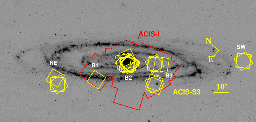
Figure 1: The field of view of the ACIS-I (red dashed outline) merged observations and ACIS-S3 chips (yellow) for each observation used in our analysis overlaid on a Spitzer 24 $\micron$ image of M31 (Gordon et al., 2006). Far left is the northeast region (NE), the bulge region is approximated by the red dashed outline (includes the ACIS-S observations within it), and the southwest region is far right (SW). The bulge region is additionally labelled into 3 separate regions based on the distribution of ACIS-S observations, bulge 1 (B1), bulge 2 (B2), and bulge 3 (B3). B3 includes the observations overlapping M32 as well as the fields just above it.

Table 3: ACIS-S Observations

ObsID	Date	R.A.	Decl.	Distance	Livetime	Datamode	CCDs	Roll Angle	Region	$\delta x$	$\delta y$	Rotation	Scale Factor	Matched Sources	Catalogue
		(J2000)		($\arcmin$)	(ks)			($\degr$)		(Pixels)	(Pixels)	($\degr$)
(1)	(2)	(3)	(4)	(5)	(6)	(7)	(8)	(9)	(10)	(11)	(12)	(13)	(14)	(15)	(16)
309	2000-06-01	10.68800	41.27877	0.6	5110	FAINT	235678	87.5	B2	-0.16364	-0.26018	-0.03257	0.99909	4	CFHT
310	2000-07-02	10.68311	41.27876	0.6	5263	FAINT	235678	108.7	B2	0.36313	-0.19187	0.10652	1.00187	8	CFHT
313	2000-09-21	10.65816	40.87837	23.5	5980	FAINT	235678	162.9	B3	0.48271	-0.96208	0.03642	1.00353	3	2MASS
314	2000-10-21	10.64900	40.86757	24.1	5190	FAINT	235678	209.4	B3	0.49169	-1.32084	0.05563	1.00032	6	X-ray
2052	2000-11-01	11.53802	41.65947	45.0	13878	FAINT	235678	226.9	NE	-0.00785	-0.60853	0.08427	1.00164	4	CFHT
2046	2000-11-05	9.62713	40.26241	77.2	14767	FAINT	235678	237.6	SW	1.25572	-0.05402	-0.10691	0.99895	8	X-ray
2049	2000-11-05	10.44879	40.98187	20.2	14572	FAINT	235678	236.1	B3	-0.42443	0.56398	-0.23159	1.00028	5	2MASS
1580	2000-11-17	10.66379	40.85630	24.8	5407	FAINT	235678	251.5	B3	0.42793	-0.92874	0.19477	1.00102	4	2MASS
1854	2001-01-13	10.67349	41.25548	0.9	4697	FAINT	235678	295.6	B2	-0.65829	-0.27766	0.09229	1.00050	5	CFHT
2047	2001-03-06	9.69689	40.27309	74.7	14591	FAINT	235678	330.4	SW	2.11548	-1.17785	-0.01302	0.99931	7	X-ray
2053	2001-03-08	11.61538	41.66618	48.2	13363	FAINT	235678	330.5	NE	0.25278	-1.17593	-0.09831	0.99927	4	CFHT
2050	2001-03-08	10.51841	40.99440	18.1	13046	FAINT	235678	331.7	B3	-1.22735	-0.54781	0.06256	1.00063	4	2MASS
2048	2001-07-03	9.64190	40.33115	73.5	13779	FAINT	235678	109.6	SW	-0.25110	-0.31239	-0.10373	0.99851	4	Nomad
2051	2001-07-03	10.45902	41.05868	16.2	13583	FAINT	235678	109.0	B3	0.50294	-0.03155	-0.18985	0.99596	5	2MASS
2054	2001-07-03	11.54972	41.71649	47.3	14531	FAINT	235678	108.3	NE	-0.59834	-0.00160	-0.19307	0.99860	4	CFHT
1575	2001-10-05	10.66840	41.27894	1.0	39093	FAINT	235678	180.4	B2	0.21776	-0.65811	0.06315	1.00038	10	CFHT
2900	2002-11-29	11.16410	41.35916	22.3	5331	FAINT	136789	263.7	B1	0.00674	-1.04238	-0.15971	1.00138	4	SDSS
4541	2004-11-25	11.51934	41.70871	45.9	25631	FAINT	235678	260.0	NE	0.00551	-0.98102	-0.00539	0.99743	7	SDSS
6167	2004-11-26	11.51931	41.70871	45.9	24230	FAINT	235678	260.0	NE	0.76975	-0.25521	-0.04166	1.00155	7	SDSS
4536	2005-03-07	10.46483	40.93912	22.1	56181	FAINT	235678	330.4	B3	0.24710	-2.32722	-0.09497	1.00424	3	X-ray
14197	2011-09-01	10.68124	41.26788	0.2	37465	FAINT	235678	143.6	B2	-0.18277	-0.08271	0.01628	0.99981	7	CFHT
14198	2011-09-06	10.68135	41.26769	0.2	39875	FAINT	235678	147.7	B2	-0.22336	0.35097	-0.00697	1.00107	9	CFHT
13825	2012-06-01	10.68170	41.27070	0.2	39791	FAINT	23567	87.7	B2	-0.09198	0.00991	0.03199	1.00160	8	CFHT
13826	2012-06-06	10.68155	41.27051	0.2	36681	FAINT	235678	91.9	B2	-0.32372	-0.29423	0.03545	1.00100	9	CFHT
13827	2012-06-12	10.68139	41.27031	0.2	41481	FAINT	235678	96.2	B2	0.12455	1.22787	-0.10924	1.00182	8	CFHT
13828	2012-07-01	10.68111	41.26974	0.2	39881	FAINT	235678	107.9	B2	-0.06387	-0.33627	0.02094	1.00162	8	CFHT
14195	2012-08-14	10.68103	41.26846	0.2	27891	FAINT	235678	132.2	B2	0.49410	0.38553	-0.00897	1.00107	10	CFHT
15267	2012-08-16	10.68105	41.26846	0.2	11103	FAINT	235678	132.2	B2	0.41818	-0.28493	0.01966	0.99979	8	CFHT
14196	2012-10-28	10.68565	41.26598	0.2	42851	FAINT	23567	221.7	B2	-0.02078	-0.09118	0.05369	1.00091	10	CFHT

• The R.A. (column 3) and Decl. (column 4) represent the pointing of the optical axis, the RA_PNT and DEC_PNT keywords from the level-2 events files. Distance (column 5) represents the distance in arcminutes of the observation’s pointing (RA_PNT and DEC_PNT) from the centre of M31 (J004244.33+411607.50). Livetime (column 6) is the total amount of time that CCDs actually observe a source, which excludes the dead time (e.g. time it takes to transfer charge from the image region to the frame store region). CCDs (column 8) indicates the CCD chips that were on during the observation, where for ACIS-S we only used chip 7 (S3) for analysis. Region (column 10) defines one of the 5 ACIS-S regions in Figure 1: northeast (NE), left (northeast) of the bulge (B1), bulge centre (B2), right (southwest) of the bulge (B3), and southwest (SW). Columns $11-16$ summarize the results from matching each ObsID to a reference astrometric catalogue (see Section 2.2 for details) using the CIAO tool wcs_match.

Table 4: ACIS-I Observations

ObsID	Date	R.A.	Decl.	Distance	Livetime	Datamode	CCDs	Roll Angle	$\delta x$	$\delta y$	Rotation	Scale Factor	Matched Sources	Catalogue
		(J2000)		($\arcmin$)	(ks)			($\degr$)	(Pixels)	(Pixels)	($\degr$)
(1)	(2)	(3)	(4)	(5)	(6)	(7)	(8)	(9)	(10)	(11)	(12)	(13)	(14)	(15)
303	1999-10-13	10.67806	41.26989	0.3	11839	FAINT	012367	193.0	-0.18797	0.16872	0.02523	0.99995	15	CFHT
305	1999-12-11	10.68273	41.26395	0.3	4131	FAINT	01236	274.0	-0.26412	0.36347	0.02543	0.99911	12	CFHT
306	1999-12-27	10.68409	41.26370	0.3	4134	FAINT	01236	285.4	-0.00194	-0.34534	0.03549	1.00060	12	CFHT
307	2000-01-29	10.68116	41.25783	0.7	4118	FAINT	01236	304.3	-0.14524	-0.12621	0.02251	0.99985	15	CFHT
308	2000-02-16	10.68763	41.25244	1.0	4015	FAINT	012356	315.0	-0.02836	-0.76721	-0.03976	1.00036	13	CFHT

• The R.A. (column 3) and Decl. (column 4) represent the pointing of the optical axis, the RA_PNT and DEC_PNT keywords from the level-2 events files. Distance (column 5) represents the distance in arcminutes of the observation’s pointing (RA_PNT and DEC_PNT) from the centre of M31 (J004244.33+411607.50). Livetime (column 6) is the total amount of time that CCDs actually observe a source, which excludes the dead time (e.g. time it takes to transfer charge from the image region to the frame store region). CCDs (column 8) indicates the CCD chips that were on during the observation, where for ACIS-I we used chips 0123 (I0-I3) for analysis. Also, ObsID’s 1581/82 only had 2 active CCDs. Columns $10-15$ summarize the results from matching each ObsID to a reference astrometric catalogue (see Section 2.2 for details) using the CIAO tool wcs_match. We do not classify ACIS-I observations by region since they are contiguous. (This table is published in its entirety in the electronic edition of the journal. A portion is shown here for guidance regarding its form and content.)

2.2 Image Registration

While Chandra has absolute astrometry of $\approx 0.6\arcsec$ (90 per cent uncertainty circle, within 3′ of the aimpoint), creating an X-ray point source catalogue requires more precision. Therefore we performed alignment to a ground-based standard for every ACIS observation to improve astrometry to the extent possible. We began by using a wide-field image that covers the PHAT-fields (Williams et al., 2014) obtained with the Canada-France-Hawaii Telescope (CFHT) MegaPrime/MegaCam in the $i$ (MP9701) filter. The astrometry in this image had already been corrected to match the Two Micron All Sky Survey (2MASS, Skrutskie et al. 2006) reference system, which is accurate to $<0.2\arcsec$. We used this image because the PHAT data was aligned to it, therefore making optical counterpart identification more precise. We used the daofind tool in the IRAF\DAOPHOT package (Stetson, 1987) to compile a source list from the CFHT image. We chose sources in the CFHT image that were either background galaxies or globular cluster LMXB sources. For the datapars settings we changed the $\it{fwhmpsf}$ parameter to 2 based on an analysis of numerous point sources in the image. The $\it{sigma}$ (the standard deviation of the mode of the background), $\it{datamin}$, and $\it{datamax}$ parameters were all calculated from the image; the $\it{readnoise}$ was set to 5. For centerpars the $\it{calgorithm}$ was set to centroid, while the fitskypars parameter $\it{salgorithm}$ was set to median and $\it{annulus}$ and $\it{dannulus}$ were both set to 8 ($4\times$ $\it{fwhmpsf}$). The photpars parameter $\it{zmag}$ was set to 25.72, the zero point of the magnitude scale for the $i$ filter on the CFHT MegaPrime/MegaCam. The findpars settings were left to their defaults. We ran the phot procedure with the above settings to determine precise centroids for our output source list.

We used the CIAO tool wcs_match to match and then align the X-ray source list (from the full energy band) for an observation to the reference source list created using IRAF\DAOPHOT from the CFHT image. We set the search radius to $2\arcsec$ and use the WCS from the input (X-ray) source list since the program requires WCS parameters to specify a tangent point for the transform calculations. To eliminate matches with large positional errors from the final transformation calculation, we disabled the $\it{residlim}$ parameter (set to 0), set the $\it{residtype}$ parameter to 0, and set the $\it{residfac}$ parameter to 25. If any residual-to-source pair position error ratio exceeds the value of $\it{residfac}$ it is omitted from the transformation calculation, where the $\it{residtype}$ parameter setting ensures this is completed for each individual source-pair as opposed to averaging all source-pairs. The program then created a transformation matrix with $x$ and $y$ offsets (R.A. and decl.) as well as a rotation and scale parameter. This matrix was then used with wcs_update to correct the astrometry of the aspect solution file for each individual observation. Since we reprocessed each observation from the level-1 events file, which specifies events in chip coordinates, only the aspect solution file needed to be corrected since it provides the appropriate WCS for acis_process_events to convert from chip coordinates to sky coordinates. A complication arose during matching that stems from the exposure mode for many of our observations. The majority of observations were completed in interleaved mode (known as alternating exposure mode), which is carried out by alternating short and long frame times. Two separate event files are produced, one representing events with long frame times and another the short frame times. This is advantageous when observing sources that may be piled-up, such as those in the nucleus of M31. The event files with short frame times all have small livetime exposures and therefore it was difficult to find matching sources for alignment. Since the event files with long frame times always had much larger livetime exposures, they provided more precise astrometric alignment because more sources were detected. Therefore we used the same transformation matrix from the long frame time event file to correct the astrometry for the short frame time event file.

However, 10 ACIS-I and 13 ACIS-S observations were either outside of the PHAT-field or did not have at least three source-pair matches to CFHT image sources. For these observations we first attempted to introduce more matches by using a source list of galaxies from the Sloan Digital Sky Survey (SDSS) Data Release 10. We obtained the source list through the CasJobs batch query service because it has no limit on the number of rows output. In the cases where the SDSS match failed, we introduced stars found in the SDSS, whose positions are not necessarily as precise because they may be subject to large proper motions (foreground stars). The proper motions of matched stars that were available were found to be negligible ($<5$ mas yr^-1). Lastly, we introduced a source list of galaxies from the Two Micron All Sky Survey (2MASS) All-Sky Point Source Catalogue. Since 2MASS publishes an error ellipse, we used $\sqrt{a\times b}$ to determine the error for R.A. and Decl., where $a$ and $b$ are the semi-major and semi-minor axes. The remaining ACIS-I observations were all aligned with the inclusion of the 2MASS point sources. However, 5 ACIS-S observations (314, 4536, 2046, 2047, and 2048) still had $<3$ reliable matches. We then included stars from the Naval Observatory Merged Astrometric Dataset (Zacharias et al., 2005), which also mostly appeared in the SDSS catalogue. This helped us align observation 2048, where we were careful to check that the proper motions of the matched stars were negligible. For the last 4 observations we merged the wavdetect X-ray source lists from the soft, hard, and full energy bands and repeated the matching procedure above with no success. Since many of our observations overlap one another, we used the astrometric alignments calculated to update the wavdetect X-ray source lists from observations that overlapped the 4 that were still unaligned. This method was still unsuccessful for observation 4536, and so it maintains its original astrometry. The details of astrometric alignment are summarized in Tables 3 and 4.

2.3 Merging

We needed to create merged images of each M31 region (northeast, bulge, southwest) in order to detect the faintest sources. After correcting the astrometry in each individual observation by updating the aspect solution file, we repeated the same preliminary reduction process for events files outlined in Section 2.1 with one minor change: we enabled the energy-dependent subpixel event repositioning algorithm in acis_process_events to improve the spatial resolution of point sources on-axis. This algorithm is useful to later distinguish nearby X-ray point sources since most of the observations are centred on the nucleus of M31, and point sources are denser in this region of the galaxy. We then reprojected the cleaned event files for all 29 ACIS-S and 104 ACIS-I observations using reproject_obs. Reprojections were made to the tangent points of the longest observations within the given region. We then created exposure maps and exposure-corrected images (photons cm^-2 s^-1 pixel^-1) for each observation with the flux_obs tool, which combined them to create an exposure-corrected image of the 104 ACIS-I observations in the bulge and 5 exposure-corrected images of the various 29 ACIS-S observations based on their overlapping fields (northeast and southwest regions, and 3 regions in the bulge: nucleus and left (northeast) and right (southwest) of the nucleus; see Figure 1). The right (southwest) bulge field has 2 ACIS-S regions that we combined due to their proximity. We used a binsize of 1 to maintain the native resolution and weighted spectrum files (corresponding to the soft, hard, and full energy bands) to calculate instrument maps.

We created a total of 18 images throughout the soft, hard, and full energy bands, 3 ACIS-I and 15 ACIS-S, with each representing the regions in Figure 1. The plate scale of the Chandra images is 0.5 arcsecond pixel^-1, corresponding to 1.9 pc pixel^-1 at the distance of 776 kpc for M31 adopted at the end of Section 1. Chandra ACIS has spatial resolution that ranges from 1″ on-axis to 4″ at 4′ off-axis for 1.5 keV X-rays at 90 per cent encircled energy fraction. The 3 ACIS-I images of the bulge were each $\approx 150$ MB and had dimensions of 5824 pixels by 6145 pixels. Executing flux_obs and wavdetect to create this image and detect sources required a large amount of memory (e.g. $\sim 25$ GB for ACIS-I image creation) and storage space ($>1$ TB for all data and ancillary files). We used the Canadian Advanced Network for Astronomical Research (CANFAR; Gaudet et al. 2011) to complete this processing.

2.4 Source Catalogue Creation

Source detection was accomplished using wavdetect in order to create a preliminary list of source positions. Starting from our merged exposure-corrected images (one ACIS-I region and five ACIS-S regions) in the soft, hard, and full bands, we used the $\sqrt{2}$ series from 1 to 8 for the scales parameter, corresponding exposure maps to reduce false positives, and the inverse of the number of pixels in an image for the sigthresh parameter as recommended by the Chandra X-ray Center. Since our merged images are larger than the standard $1024\times 1024$ pixels for most images, the sigthresh parameter needed to be modified to reduce the number of false sources detected. It was set to $3\times 10^{-8}$ for the ACIS-I image and $\sim$few$\times 10^{-6}$ for the five ACIS-S images. The expthresh parameter was changed from its default value of 0.1 to 0.001 for all 6 merged images. Pixels with a relative exposure (pixel exposure value over maximum value of exposure in the map) less than expthresh are not analysed, and adopting the default value would exclude the analysis of many of the low-exposure regions in our merged images. All other wavdetect parameters were left at their default values. The source lists we obtained were then combined into a master source list using the match_xy tool from the Tools for ACIS Review and Analysis (TARA) package, resulting in a candidate list of 1068 sources. In addition, to ensure all possible sources were detected reproject_image was used to merge the 3 ACIS-S bulge region counts images with the ACIS-I counts image. Running wavdetect on each energy range for this master bulge region image and combining the source lists following the same procedure as above we recovered 331 additional sources (unique from the original 1068). Therefore we had a total of 1399 wavdetect sources.

To obtain source properties from our preliminary list of source positions we used ACIS Extract (AE; Broos et al., 2010), which performed source extraction and characterization. AE analyses the level-2 event files of each observation individually before merging and determining source properties. In order to create a reliable catalogue, we followed the methods outlined in the validation procedure used by the authors of AE. This multi-step process (summarized in Figure 1 of Broos et al. 2010) involved many iterations of extracting, pruning, and repositioning sources in the candidate catalogue. We pruned sources using the AE parameter $pns$ (‘$prob\_no\_source$’ or the p-value for no-source hypothesis), which calculates the Poisson probability of a detection not being a source by taking the uncertainty of the local background into account. Using the $pns$ value removes the bias inherent in using the traditional $3\sigma$ source significance criterion, where sources with low count rates would have been left out.

Before pruning any source we visually inspected it in any of the observations it appeared to be sure that it was insignificant. In some cases 2 neighbouring sources were both selected for pruning, but it was often found that either one would survive if the other was removed. The most advantageous aspect of the validation procedure was the ability to review each source and select the most likely position based on the properties of an individual source. Specifically, the repositioning stage displays the original catalogue position and also calculates 3 other position estimates: the mean data, correlation, and maximum-likelihood reconstruction positions. The catalogue and/or centroid positions were used most often, but for sources with large off-axis angles ($\gtrsim 5\arcmin$) the correlation position was used, whereas for crowded sources with overlapping PSFs the maximum-likelihood reconstruction position was used (see §7.1 of Broos et al. 2010 for a detailed description of source positions). AE also produces smoothed residual images for each observation, which are the smoothed residuals remaining after the point source models are subtracted from the observation data. The residual image is scaled to emphasize only bright residuals, which are possible sources that may have been missed by wavdetect or were accidentally pruned. Inspecting the observed events and point source model for a bright residual reveals whether it is an artefact or likely point source. We found 43 sources using the residual images that were added to our source list. After catalogue positions were validated, the one-pass photometry procedure (follows the validation procedure, see footnote 6) completed the final extraction for all 795 sources in our final M31 catalogue; output source properties are summarized in Tables 5$-$6. To be included in the final catalogue a source was required to have a $pns$ value $\leq 1\times 10^{-2}$ (default in AE) in any of the energy bands (full, soft, or hard). We chose this value since it was used for the Chandra Carina Complex Project (Broos et al., 2011) to balance sensitivity with source detection significance. In the full band, all 795 (100%) of our sources had a $pns$ value $\leq 1\times 10^{-2}$.

3 X-ray Source Catalogue Properties

3.1 Source Catalogue

Our final M31 catalogue consists of 795 X-ray point sources. Their properties are summarized in Tables 5$-$6. The detailed FITS tables from AE, which include $\sim 100$ other source photometric properties used in AE (e.g. background region metrics) in 16 energy bands (see Section 7.8 of the AE manual for these bands), are available on the journal website. Of the 795 sources, 42 are in the northeast portion of M31, 728 are in the bulge, and 25 are in the southwest. The fluxes in Table 6 were calculated using conversion factors of 5.47, 1.86, and 3.37 in units of $10^{-9}$ erg photons^-1 for the full, soft, and hard bands (to convert from photon flux in photons cm^-2 s^-1 to energy flux in erg cm^-2 s^-1). Photon fluxes were estimated by AE (flux2 parameter) based on the number of net source counts ($net\_cts$), the exposure time, and the mean ancillary response function ($MEAN\_ARF$) in the given energy band. This flux estimate suffers from a systematic error (compared to the true incident flux) because the $MEAN\_ARF$ is the correct effective area normalization based on an incident spectrum that is flat. To obtain a more accurate flux estimate, one should sum the flux values over narrow energy bands. We performed this summation for the full, soft, and hard energy bands using the fluxes in narrow energy ranges provided by AE: $0.5-1.0$, $1.0-2.0$, $2.0-4.0$, $4.0-6.0$, and $6.0-8.0$. We found a difference of $-8$%, 5%, and 13% between the summed flux values and those from the flux2 parameter. This percent difference is much smaller than the expected uncertainties for fluxes based on the Poisson errors for the net counts. We reported the summed fluxes in the full, soft, and hard bands in the last 3 columns of Table 6. We used the AE flux2 fluxes for our analysis. We converted the photon flux into an energy flux assuming an absorbed power-law spectrum with $\Gamma=1.7$ and $N_{H}=6.66\times 10^{20}$ cm^-2 (details in Section 3.3). In Figure 2, we show histograms of the net counts (left panel) and source flux in erg s^-1 cm^-2 (right panel) for all our sources. The left panel shows sources with $<200$ counts, while the inset shows a log distribution of all sources, clearly indicating the majority of sources have $<100$ counts. The 191 sources that have $\gtrsim 200$ counts are suitable for spectral modelling. The source flux histogram shows a peak in the flux distribution near our 90% detection limit of $\approx 5\times 10^{-15}$ erg s^-1 cm^-2 ($3\times 10^{35}$ erg s^-1). The X-ray point source population of M31 is comprised of LMXBs and HMXBs, supernova remnants, and background AGNs. To determine the makeup of our population of point sources we created XLFs and used various catalogues from previous studies.

Table 5: M31 Source List

Source	CXOU J	R.A. (J2000)	Decl. (J2000)	Distance	PosErr	$\theta$	No. of	Detector	Region	Tot Exp	Tot Exp. Map	Rsrc	SNR	$E_{\rm{median}}$	Match
No.		($\degr$)	($\degr$)	($\arcmin$)	($\arcsec$)	($\arcmin$)	Obs			(ks)	Value (s cm2)	(sky pixel)		(keV)
(1)	(2)	(3)	(4)	(5)	(6)	(7)	(8)	(9)	(10)	(11)	(12)	(13)	(14)	(15)	(16)
1	004542.90+414312.6	11.428779	41.720189	43.03	0.2	4.1	2	ACIS-S	NE	49	1.14E+07	4.5	6.5	2.1
2	004551.05+414452.4	11.462750	41.747912	45.26	0.3	3.5	2	ACIS-S	NE	49	1.64E+07	3.5	2.7	2.7
3	004551.30+414220.7	11.463769	41.705754	43.74	0.2	2.8	3	ACIS-S	NE	64	2.20E+07	2.8	2.4	2.3	AGN
4	004552.93+414441.8	11.470551	41.744965	45.42	0.2	3.1	2	ACIS-S	NE	49	1.68E+07	3.0	2.8	2.0
5	004555.72+414551.8	11.482172	41.764389	46.56	0.3	3.7	2	ACIS-S	NE	49	1.67E+07	4.0	2.5	2.5
6	004556.82+414440.8	11.486787	41.744673	45.98	0.2	2.6	2	ACIS-S	NE	49	1.72E+07	2.5	2.5	2.7
7	004556.99+414831.7	11.487497	41.808829	48.48	0.2	6.2	2	ACIS-S	NE	49	1.60E+07	9.3	9.6	2.4	AGN
8	004559.07+414113.0	11.496132	41.686945	44.27	0.2	2.6	5	ACIS-S	NE	91	3.38E+07	3.0	5.3	2.9
9	004602.43+414515.7	11.510137	41.754377	47.16	0.2	3.1	3	ACIS-S	NE	63	1.84E+07	3.3	5.7	2.1
10	004602.70+413856.7	11.511251	41.649095	43.61	0.3	3.4	3	ACIS-S	NE	41	1.62E+07	4.1	3.6	1.4

• $\bf{Notes}$. Column 2: source ID, which contains the source coordinates (J2000.0). Column 5: distance in arcminutes of the source from the centre of M31 (J004244.33+411607.50). Column 6: positional uncertainty $\sqrt{\sigma_{x}^{2}+\sigma_{y}^{2}}$, where the single-axis position errors $\sigma_{x}$ and $\sigma_{y}$ are estimated from the standard deviations of the PSF in the extraction region and the number of counts extracted. Column 7: average off-axis angle for merged observations. Column 8: number of observations extracted. Column 9: source detected in ACIS-I, ACIS-S, or Both. Column 10: for a source detected in ACIS-S or Both, indicates which region from Figure 1 it belongs to. Columns 11 & 12: total values for merged observations. Column 13: average radius of the source extraction region (1 sky pixel = $0.492\arcsec$). Column 14: photometric significance (net counts / upper error on net counts) ($0.3-8.0$ keV). Column 15: background-corrected median photon energy ($0.3-8.0$ keV). Column 16: cross-match results from Section 3.4: active galactic nuclei (AGN) or low-mass X-ray binary (LMXB).
  (This table is published in its entirety in the electronic edition of the journal. A portion is shown here for guidance regarding its form and content.)

Table 6: Additional M31 Source Properties

Source	$pns$	$pns$	$pns$	$net\_cts$	$\sigma_{\rm{upper}}$	$\sigma_{\rm{lower}}$	$net\_cts$	$\sigma_{\rm{upper}}$	$\sigma_{\rm{lower}}$	$net\_cts$	$\sigma_{\rm{upper}}$	$\sigma_{\rm{lower}}$	$flux$	$flux$	$flux$	Summed $flux$	Summed $flux$	Summed $flux$
No.	($0.5-8.0$ keV)	($0.5-2.0$ keV)	($2.0-8.0$ keV)	($0.5-8.0$ keV)			($0.5-2.0$ keV)			($2.0-8.0$ keV)			($0.5-8.0$ keV)	($0.5-2.0$ keV)	($2.0-8.0$ keV)	($0.5-8.0$ keV)	($0.5-2.0$ keV)	($2.0-8.0$ keV)
(1)	(2)	(3)	(4)	(5)	(6)	(7)	(8)	(9)	(10)	(11)	(12)	(13)	(14)	(15)	(16)	(17)	(18)	(19)
1	0.00E+00	1.40E-45	1.37E-23	55.65	8.60	7.53	33.52	6.90	5.80	22.13	5.87	4.76	3.07E-14	3.97E-15	8.83E-15	2.24E-14	4.06E-15	6.43E-15
2	7.48E-12	6.96E-09	6.96E-05	13.01	4.84	3.69	7.65	3.96	2.76	5.35	3.60	2.38	5.37E-15	6.33E-16	1.65E-15	5.64E-15	6.45E-16	2.31E-15
3	2.17E-09	1.18E-08	5.55E-03	10.96	4.57	3.41	7.63	3.96	2.76	3.33	3.18	1.91	3.40E-15	4.76E-16	7.70E-16	3.02E-15	4.83E-16	9.89E-16
4	4.98E-14	1.50E-10	1.19E-05	13.32	4.84	3.69	7.79	3.96	2.76	5.53	3.60	2.38	5.46E-15	6.34E-16	1.70E-15	3.84E-15	5.92E-16	1.30E-15
5	2.19E-09	1.08E-06	2.45E-04	11.71	4.71	3.56	6.53	3.78	2.58	5.18	3.60	2.38	4.86E-15	5.34E-16	1.62E-15	4.46E-15	6.04E-16	1.65E-15
6	1.04E-13	2.88E-08	5.85E-07	11.56	4.57	3.41	5.84	3.60	2.37	5.72	3.60	2.37	4.66E-15	4.66E-16	1.74E-15	4.33E-15	4.98E-16	1.77E-15
7	0.00E+00	2.01E-41	0.00E+00	117.40	12.23	11.18	50.47	8.34	7.26	66.93	9.55	8.48	5.10E-14	4.33E-15	2.19E-14	3.73E-14	4.19E-15	1.54E-14
8	1.88E-39	1.19E-12	2.21E-28	40.21	7.54	6.45	12.37	4.71	3.56	27.84	6.46	5.35	8.61E-15	5.19E-16	4.51E-15	6.79E-15	4.64E-16	3.34E-15
9	0.00E+00	6.44E-38	1.24E-16	44.71	7.84	6.76	28.51	6.45	5.35	16.20	5.21	4.08	1.69E-14	2.12E-15	4.63E-15	1.21E-14	2.04E-15	3.74E-15
10	3.91E-18	8.90E-20	5.38E-03	21.35	5.88	4.76	17.42	5.33	4.20	3.93	3.40	2.16	1.01E-14	1.58E-15	1.43E-15	7.11E-15	1.76E-15	1.20E-15

• $\bf{Notes}$. Columns (2)-(4) represent the $pns$ values, which are the Poisson probability of a detection not being a source (discussed in Section 2.4). Columns (5)-(13) are the net counts in a given energy range with 90% upper and lower uncertainty limits. Columns (14)-(16) show the fluxes (the flux2 parameter in AE) in units of erg cm^-2 s^-1. Columns (17)-(19) are the fluxes in erg cm^-2 s^-1 calculated by summing narrow energy bands and thus avoiding systematic errors in the flux2 parameter from AE (see Section 3.1). Conversion factors were 5.47, 1.86, and 3.37 in units of $10^{-9}$ erg photons^-1 for the full, soft, and hard bands (to convert from photon flux in photons cm^-2 s^-1 to energy flux in erg cm^-2 s^-1). The conversion factors account for foreground absorption using an absorbed power-law spectrum with $\Gamma=1.7$ and $N_{H}=6.66\times 10^{20}$ cm^-2. To convert energy fluxes to luminosity in erg s^-1 multiply by $7.2\times 10^{49}\left(\frac{d}{776\rm{\,kpc}}\right)^{2}$ cm². For some sources the soft or hard band had $<0$ counts, and so uncertainties could not be determined and are represented as -99.99. By extension, some fluxes in the soft or hard band were $<0$ and so luminosities appear as -9.99. Each source has a $pns$ value $<1\times 10^{-2}$ in at least one energy band.
  (This table is published in its entirety in the electronic edition of the journal. A portion is shown here for guidance regarding its form and content.)

Figure 2: Histograms of the net source counts (left panel) and source flux (right panel) in the full energy band. The left panel shows sources with $<200$ counts while the inset shows a histogram of all 795 sources. While the majority of sources have $<200$ counts, the 191 sources (mostly in the nucleus) with $\gtrsim$200 counts are candidates for spectral modeling. In the right panel, the peak in the distribution is near our 90% detection limit of $\approx 5\times 10^{-15}$ erg s^-1 cm^-2 ($3\times 10^{35}$ erg s^-1).

3.2 Cross-Correlation With Existing Catalogues

Of the many previous studies in M31 summarized in Tables 1 - 2, not all actually publish a traditional X-ray catalogue. Approximately half the studies were focused on only one specific X-ray population. Our first comparisons are to the XMM-Newton catalogue (Stiele et al., 2011) because it is complete throughout M31 to a limiting luminosity of $\sim 10^{35}$ erg s^-1. Of the 1948 X-ray sources identified, only 979 appear within the field of view of our Chandra data. Figure 3 shows the deprojected radial distribution of X-ray sources in our catalogue (black) compared to those from the XMM-Newton survey (blue). Because our survey has sporadic coverage, only the nuclear region, where the exposure is significant, do we see a greater source density. Also, the subarcsecond resolution of Chandra allowed us to separate closely-spaced sources that XMM-Newton was unable to resolve due to its 5″ PSF.

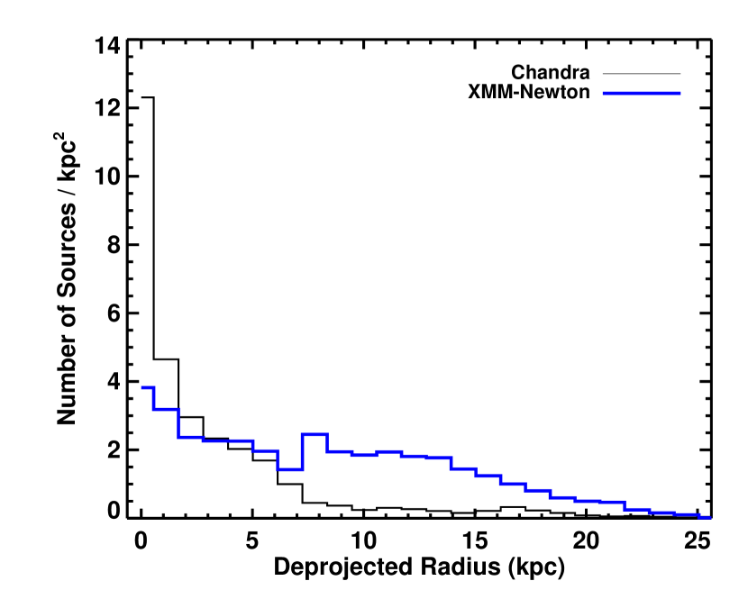
Figure 3: Deprojected radial source distribution of X-ray point sources in our catalogue (black) compared with those from the XMM-Newton survey (blue). The density of our Chandra sources drops off considerably around a few kpc because the coverage of our survey is sparse (see Figure 1). However, the deeper observations of the nucleus combined with the sub-arcsecond resolution of Chandra results in a $\sim 3$-fold increase in the number of sources within the central kpc.

We also matched our catalogue to the XMM-Newton catalogue using a matching radius of 5″, equivalent to XMM-Newton’s source positional uncertainty. We found that 352 XMM-Newton sources matched to 387 (49%) of our Chandra sources, where the 352 unique Chandra sources (closest matches) made up 44 per cent of our catalogue. Because the XMM-Newton PSF is much larger than Chandra’s, multiple Chandra sources were matched to within 5″ of an XMM-Newton source. The median offset between matches was 1.08″. In Figure 4 we show the positional offset between the matches (left panel) and compare the average fluxes from both surveys (right panel). Chandra fluxes appeared systematically brighter with a mean value of $\sim 50\%$, either due to cross-calibration between the observatories or the assumed conversion factor used for XMM-Newton fluxes. To address the sources in the XMM-Newton catalogue that were not matched to our catalogue, we compiled a list of all the original input sources throughout all three fields (1399) and included an additional $\sim 5000$ sources from a low-significance wavdetect run. Matching this list to the XMM-Newton catalogue within 5″ we find that 895 (91%) of XMM-Newton sources were matched. Therefore many sources can be identified as candidates in the Chandra observations but not ‘detected’ due to a low significance (e.g., shallow exposure, transience).

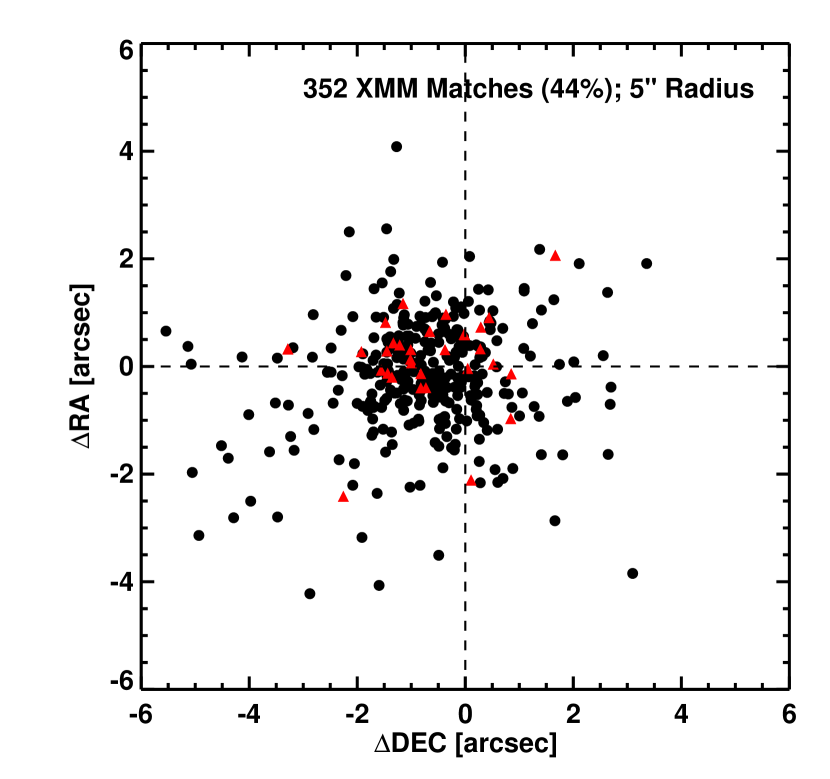
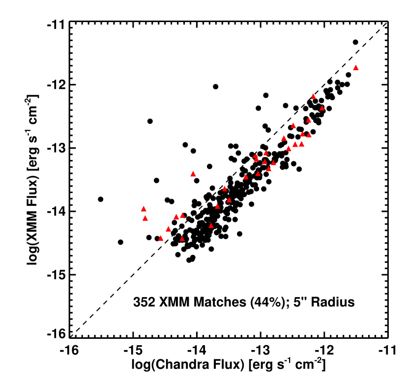
Figure 4: A comparison of the 352 (44%) unique Chandra X-ray sources (a total of 387 (49%) were matched) detected in this work that were the closest matches to those from the XMM-Newton catalogue within 5″ (approximately the positional uncertainty associated with XMM-Newton sources). The left panel shows the approximate positional offset between the matches while the right panel compares the fluxes. The red triangles represent XMM-Newton sources that were matched to multiple Chandra sources, where the values plotted came from the closest-matched source. XMM-Newton fluxes ($0.2-4.5$ keV) have been corrected to the Chandra energy range ($0.5-8.0$ keV) assuming the spectral model from Section 3.3. Chandra fluxes are $\sim 50\%$ brighter, which is due to either cross-calibration between the observatories or the assumed conversion factor used for XMM-Newton fluxes.

Our catalogue was also matched to within 1″ of previous Chandra catalogues of various X-ray sources. From the Chandra surveys in Table 2, a total of 1436 sources (some authors omitted sources from their catalogue if they were not new) were cross-matched with those from our catalogue. Among the past Chandra catalogues there is some redundancy as groups do not always exclude previously detected sources from their catalogue. Using this matching radius we find only 347 of our sources that matched to previously detected Chandra sources, with a median offset of 0.27″. 448 of our catalogue sources were detected for the first time from Chandra observations. When combining the unique matches from both XMM-Newton and previous Chandra surveys we find that 536 matched from our catalogue of 795 sources, meaning 259 of our X-ray sources were detected for the first time. These new sources have a factor of 2 smaller exposure times, a factor of three fewer counts and photon fluxes, a factor of six fewer observations per source, and $pns$ values that are twelve orders of magnitude less significant, when compared to median values of the whole catalogue (e.g. $pns\approx 10^{-17}$). When compared to only the matched sources, these differences are exacerbated even more so. Matching results are shown in Table 7. The cross-match information between our catalogue and previous XMM-Newton and Chandra catalogues, including their identification numbers/values (where available), is shown in Table 8. We also show the number of our catalogue sources matched for each source classification type from other catalogues in Table 9.

Table 7: Matching Results

	XMM-Newton	Previous Chandra	Total Matched	New sources
This work (795)	387 (352 unique)	347	536	259

• A 5″ radius was used for matching to XMM-Newton, while a 1″ radius was used when matching to previous Chandra catalogues. 387 of our catalogue sources were matched to 352 XMM-Newton sources.

Table 8: X-ray Catalogue Cross-Matches

Source	CXOU J	XMM-Newton Match		Chandra Match		LMXB Match			AGN Match
No.		ID	Classification	Catalogue	ID	Peacock et al.; GC	Stiele et al.; Field	Stiele et al.; GC	PHAT	SDSS DR12	NED	SIMBAD
(1)	(2)	(3)	(4)	(5)	(6)	(7)	(8)	(9)	(10)	(11)	(12)	(13)
1	004542.90+414312.6	1685	$<$hard$>$	-	-	-	-	-	-	-	-	-
2	004551.05+414452.4	-	-	-	-	-	-	-	-	-	-	-
3	004551.30+414220.7	-	-	-	-	-	-	-	3900	-	-	-
4	004552.93+414441.8	-	-	-	-	-	-	-	-	-	-	-
5	004555.72+414551.8	-	-	-	-	-	-	-	-	-	-	-
6	004556.82+414440.8	-	-	-	-	-	-	-	-	-	-	-
7	004556.99+414831.7	1716	$<$hard$>$	-	-	-	-	-	1938	-	-	-
8	004559.07+414113.0	-	-	-	-	-	-	-	-	-	-	-
9	004602.43+414515.7	1732	$<$SNR$>$	-	-	-	-	-	-	-	-	-
10	004602.70+413856.7	-	-	-	-	-	-	-	-	-	-	-

• $\bf{Notes}$. This table summarizes the details of the cross-match between our catalogue and various others. Columns (1) and (2) represent our catalogue. Columns (3) and (4) are the XMM-Newton catalogue identification number and classification. Column (5) is the Chandra catalogue matched to: BA (Barnard et al., 2014), DS02 (Di Stefano et al., 2002), DS04 (Di Stefano et al., 2004), HO (Hofmann et al., 2013), KA (Kaaret, 2002), KO (Kong et al., 2002), VO (Voss & Gilfanov, 2007), WI (Williams et al., 2004). Column (6) is the catalogue source identification value taken from each respective paper. Columns (7)-(9) represent matches to LMXBs from Peacock et al. (2010b) globular clusters (GC), and Stiele et al. (2011) field and globular clusters (GC), with the corresponding names or identification number. Columns (10)-(13) show the results of AGN matching to various catalogues. For PHAT, we used the Andromeda project identification number from Johnson et al. (2015). See Section 3.4 for more details on matching.
  (This table is published in its entirety in the electronic edition of the journal. A portion is shown here for guidance regarding its form and content.)

Table 9: Summary of X-ray Catalogue Cross-Matches

Source Classification	Number Matched	Number Matched (including candidates)
AGN	29	40
XRB	8	33
Globular Cluster (LMXB)	46	54
Supernova Remnant (SNR)	12	14
Foreground Star	6	29

• Total number of sources from our catalogue matched to previously identified sources from catalogues listed in Table 8. The last column includes the sources from Stiele et al. (2011) that were identified as candidates in addition to the confirmed sources (second column) from all other catalogues.

3.3 Sensitivity Curve

In order to create corrected XLFs (log$N$-log$S$) we had to evaluate the sensitivity of each point in the survey field, which gives the energy flux at which a source would be detected. Complications arise when attempting to compute sensitivity for overlapping observations/regions, which are prevalent in our survey field. In addition, the CIAO tools are not designed for this type of analysis and also do not accommodate combining ACIS-I/S observations. Therefore we take a statistical approach and follow the method of Georgakakis et al. (2008) to determine the sensitivity throughout the survey field. The source extraction process in AE estimates the Poisson probability that the observed counts in the detection cell arise completely from random fluctuations of the background. The three parameters that define this process are the size and shape of the detection cell and the Poisson probability threshold $P_{thresh}$ (AE value $pns$). The size and shape of the detection cell are defined by AE for each source based on the count distribution, source crowding, off-axis angle. By setting $P_{thresh}$ to $1\times 10^{-2}$ for our analysis, which is the AE default value, we set the minimum number of photons required in a detection cell to be considered a source.

With the parameters of the source extraction process in hand, two additional data products are needed to proceed: an exposure map and a background map. The exposure map is the total exposure at any point in the field. We created 3 exposure maps from our existing data products for 3 separate regions of the M31 field: the northeast, bulge, and southwest. In the bulge, we merged the ACIS-I/S exposure maps using the CIAO tool reproject_image to reproject the maps to a common tangent plane and merge them. The background maps were required to be identical in size to the exposure maps and so we generated 3 maps for each of the regions as for the exposure maps.

Figure 5: Sensitivity curves in the soft and hard energy bands for the complete Chandra survey area in M31. Sensitivity for the various overlapping observations and different fields was calculated using the method of Georgakakis et al. (2008). Unabsorbed fluxes and luminosities are shown assuming an absorbed power-law spectrum with $\Gamma=1.7$ and $N_{H}=6.66\times 10^{20}$ cm^-2 (see Section 3.3 for more details).

The background map is an estimate of the source-free background across the different regions in the survey. We started by using the merged counts images in each region (created in the same manner as the merged exposure maps). We removed the counts in the vicinity of detected sources using an aperture 1.5 times larger than the 90 per cent enclosed PSF radius (obtained from AE). These pixel values were replaced by the background values calculated by AE for each source. We now had an image in units of counts where we have removed the contribution from all detected sources. However, the background map should have units of counts pixel^-1 so that every pixel in the survey field has a background value associated with it. This was required for us to estimate the sensitivity at each pixel. Such an image is created by using the CIAO tool dmimgpm, which calculates a modified Poissonian mean for each pixel using a box of width 64″ as the sampling region around that pixel.

Using the background map values we estimated the minimum number of counts required in each pixel for a detection (above our threshold $P_{thresh}$) with the inverse survival function (Python version 2.7.8; scipy.stats.poisson module version 0.14.0). We then estimated the mean expected number of counts ($T=S+B$) that would be produced at each pixel for a range of fluxes. $B$ is the background value of the pixel and $S$ is the mean expected source contribution (equation (5) of Georgakakis et al. 2008). Finally, we estimated the probability that a given flux would produce the mean expected number of counts above the minimum counts required for a detection in each pixel using the survival function (python scipy.stats.poisson module). To correct our log$N$-log$S$ relations to represent the number of sources at a given flux per deg^-2 we created an area curve. This was accomplished by summing the probabilities for each pixel at a given flux to obtain the total area, which when done for the various flux values in the soft and hard energy bands gave the area curves shown in Figure 5.

As in Stiele et al. (2011), we assumed an absorbed power-law spectrum with $\Gamma=1.7$ and chose $N_{H}=6.66\times 10^{20}$ cm^-2 (Dickey & Lockman, 1990), which was the weighted average for a 1 degree radius cone around the M31 nucleus. This model matches what we expect from XRBs and background AGN in M31. As Tüllmann et al. (2011) point out, the model fails for extremely hard (soft) sources by overestimating (underestimating) the flux, but does not bias the log$N$-log$S$ relation to systematically higher or lower fluxes. In addition, most of the previous M31 surveys have used the same $\Gamma$ value and a similar Galactic foreground absorption, therefore making comparisons more accurate. We summarize the completeness limits for our survey in Table 10.

Table 10: Completeness Limits

Completeness	Full [$0.5-8.0$ keV]	Soft [$0.5-2.0$ keV]	Hard [$2.0-8.0$ keV]
50%	0.66	0.20	0.33
70%	1.37	0.45	0.69
90%	4.05	1.58	1.98
95%	6.73	2.68	3.29

• Completeness limits in various energy bands calculated from our sensitivity curves. Values show unabsorbed luminosities in units of $10^{35}$ erg s^-1.

3.4 The log$N$-log$S$ Relation and X-ray Luminosity Functions

The log$N$-log$S$ relation is calculated by determining the cumulative number of sources $N(>S)$ above a given flux $S$ (in erg s^-1 cm^-2) that are found in a survey with a total geometric area $A$:

$$N(>S) =\sum_{S_{i}>S}\frac{1}{A(S_{i})}$$ (1)

The value $N(>S)$ has units of sources deg^-2 and is weighted by the survey area over which a source with flux $S$ could have been detected. We constructed log$N$-log$S$ distributions for the soft ($0.5-2.0$ keV) and hard ($2.0-8.0$ keV) bands using all 795 sources in our catalogue with calculated fluxes in the given band. These XLFs are shown in Figure 6. We show both the uncorrected (grey) and completeness-corrected (black) data, which indicates the level of completeness of our survey in each band at the turnover of the grey curve, similar to the values in Table 10. We calculated $1\sigma$ uncertainties for our XLFs using Poisson statistics (Gehrels, 1986). We have only accounted for foreground (Galactic) extinction in computing our fluxes and therefore any internal extinction in M31 would push our curves right towards brighter fluxes. We also plot the expected contribution from AGN using the distribution of AGN from the 4 Ms Chandra Deep-Field South (CDF-S) survey (Lehmer et al., 2012). The curve is shown in red with corresponding uncertainties. As expected, the hard-band XLF shows a significant contribution from expected AGN across the entire flux range. Near the 95 per cent completeness limit of $3.29\times 10^{35}$ erg s^-1, the AGN contribution overtakes the corrected curve, possibly a result of cosmic variance from the CDF-S survey.

In Figure 7 we plot the AGN-subtracted completeness-corrected curve (blue) to represent the X-ray sources that belong to M31. We matched our detected X-ray sources in each band to a catalogue of LMXBs in M31 to within 1″. The catalogue consisted of 26 confirmed globular cluster X-ray sources and 10 confirmed field LMXBs from Stiele et al. (2011), along with 45 confirmed LMXBs from Peacock et al. (2010b). The XLF of known LMXBs is shown in gold. We cannot produce an XLF curve for HMXBs because none have been confirmed in M31. We also used several catalogues of background galaxies/AGN to match to our X-ray point sources within 1″. These catalogues include the 2270 background galaxies from the PHAT survey (Johnson et al., 2015), 1870 background quasars identified with the LAMOST survey (Huo et al., 2010, 2013, 2015), and radial searches of 2 degrees around the M31 centre in NED, SIMBAD, and SDSS DR12. The known AGN are represented by the purple curve in Figure 6. In Table 5 we have indicated if one of our catalogue sources was matched to an AGN or LMXB. We have also added the detailed cross-match information with the various AGN/LMXB catalogue identifications (where available) to Table 8. In both energy bands, the brightest sources have a significant contribution from LMXBs, whereas the known AGN are only identified for fainter fluxes. The break in the XLFs is observed at $\approx 1.3\times 10^{37}$ erg s^-1, similar to results from previous work. Stiele et al. (2011) found that $\sim 65$ per cent of sources in their M31 catalogue had no confirmed optical counterparts, which is reflected in the lack of known LMXB/AGN sources. The gap in the AGN-subtracted completeness-corrected curve (blue) in the hard band occurs in the region of our 95% completeness limit as well as where the CDF-S curve turns over. The background AGN population as measured from the CDF-S accounts for all of the sources in our flux range in both the soft and hard bands. However, the gap in the blue curve in the hard band is likely due to the uncertainties in the CDF-S that do not include cosmic variance, biasing the results from the CDF-S.

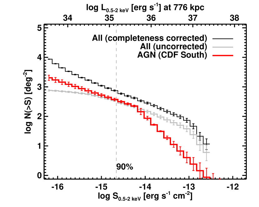
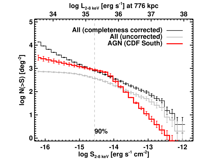
Figure 6: Cumulative number counts for the soft and hard energy bands. Both uncorrected (grey) and completeness-corrected curves (black) are plotted using all X-ray point sources with calculated fluxes in the given energy band from our catalogue. All uncertainties are $1\sigma$ (Gehrels, 1986). The AGN number counts from the 4 Ms Chandra Deep-Field South survey (Lehmer et al., 2012) are shown in red with their corresponding uncertainties. The 90% completeness limit is marked by the dashed vertical line. The red curve overtakes the black curve around the 95% completeness limit in the hard band, indicating that the majority of sources near this flux are AGN. The flattening observed (where the XLF turns over) begins at $\approx 1.3\times 10^{37}$ erg s^-1 and is consistent with previous results from M31 (Kong et al., 2002).

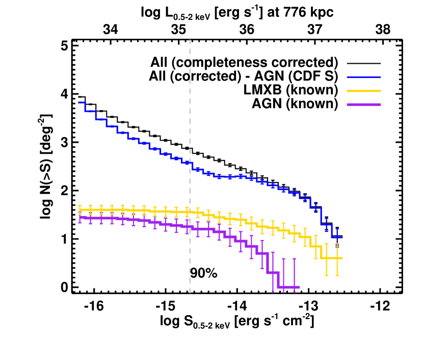
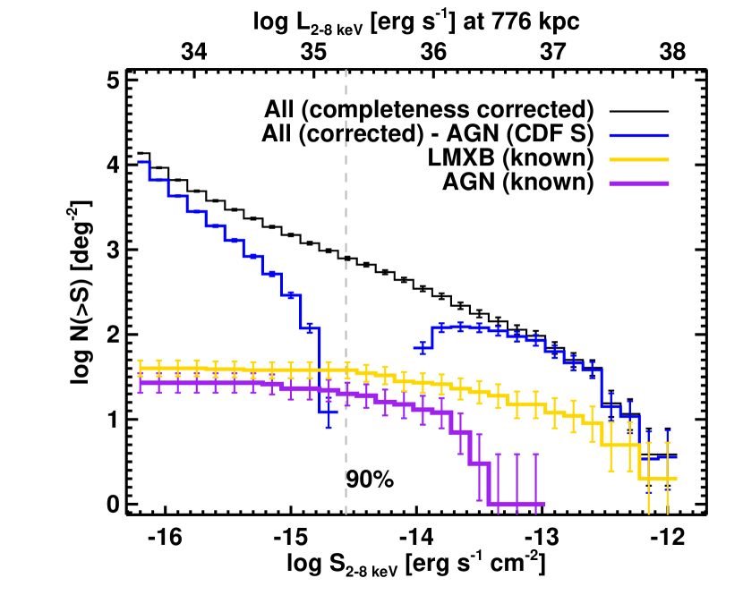
Figure 7: Cumulative number counts for the soft and hard energy bands. The completeness-corrected curve (black) is plotted using all 795 X-ray point sources from our catalogue. Known LMXBs have been matched to within 1″ of our point sources and their XLF is shown in gold. We also used various observational catalogues of known AGN and background galaxies to match within 1″ of our point sources, with their XLF shown in purple. The blue curve shows our completeness-corrected curve after subtracting the contribution from AGN CDF-S (red curve from Figure 6). All uncertainties are $1\sigma$ (Gehrels, 1986). The 90% completeness limit is marked by the dashed vertical line. As Stiele et al. (2011) pointed out, many sources in M31 have no confirmed optical counterparts; this is reflected in the lack of known sources. The background AGN population as measured from the CDF-S accounts for all of the sources in our flux range in both the soft and hard bands. The gap in the blue curve in the hard band is likely due to the uncertainties in the CDF-S, which do not include cosmic variance, biasing the results from the CDF-S (our 95% completeness limit is also located in this region).

In addition to our XLFs for all our sources, we also divided our sample to study the bulge and disk fields in M31. In Figure 8, we show the soft and hard band XLFs for these regions. Courteau et al. (2011) found that the M31 bulge light dominates for $R_{min}\lesssim 1.2$kpc, which represents the projected minor axis radius. The disk dominates in the range 1.2 kpc $<R_{min}<$ 9 kpc, and the halo beyond that. We include the disk$+$halo curve in our XLF (represented by the $R_{min}>1.2$ kpc curve) because there is no change in the XLF when excluding the halo sources as defined in Courteau et al. (2011). In the soft band, the bulge has a larger number of brighter sources (this may be biased due to the incompleteness of disk data), although the number is still within the statistical uncertainties compared to the disk$+$halo. In the hard band, the disk$+$halo harbours the brightest sources but again the bulge has a larger cumulative number of bright sources above the break at $\approx 1.3\times 10^{37}$ erg s^-1. The flatter bulge XLFs in both bands are consistent with previous results from M31 (e.g. Kong et al., 2002; Williams et al., 2004). The M31 XLF is different from other galaxies (e.g. Colbert et al., 2004; Binder et al., 2012) in that the older stellar population in the bulge has a flatter slope than the younger stellar population in the disk. The lack of bright sources and steeper XLF in the disk indicates that star formation in the disk is low, and thus any HMXBs would be faint (likely a reason none have yet been confirmed). Using XMM-Newton, Trudolyubov et al. (2002) analysed the bulge and two northeast fields and found the disk and bulge XLFs to have a similar slope, but using a 15′ radius for the bulge. They did find that disk sources are all fainter than $2\times 10^{37}$ erg s^-1, while brighter bulge sources existed.

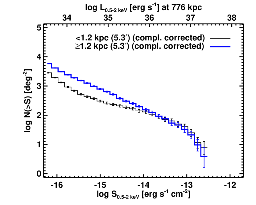
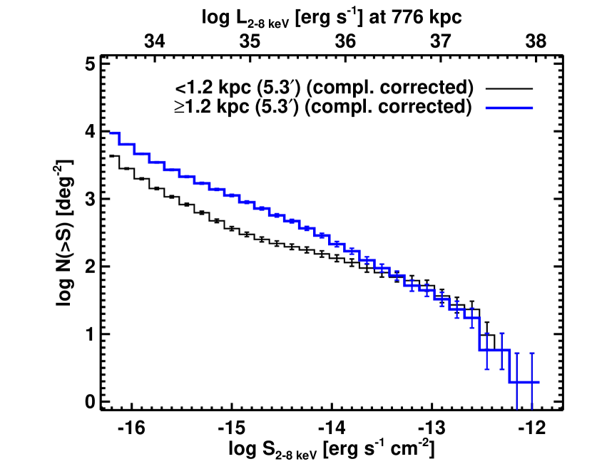
Figure 8: Cumulative number counts for the soft and hard energy bands in the bulge (black) and disk$+$halo (blue) fields of M31. The completeness-corrected curves have uncertainties of $1\sigma$ (Gehrels, 1986). The bulge and disk$+$halo populations were separated using projected radii based on the results of Courteau et al. (2011). In the soft band, the bulge has a larger number of brighter sources (although this may be biased due to the incompleteness of disk data), which is unexpected for an older stellar population. However, both curves are similar within uncertainties near the bright-end. In the hard band the disk$+$halo harbours the brightest sources but again the bulge has a larger cumulative number of bright sources above the break at $\approx 1.3\times 10^{37}$ erg s^-1. The flatter bulge XLFs in both bands are consistent with previous studies.

XLF’s have been produced for the M31 X-ray population in a number of different Chandra surveys. Kong et al. (2002) found 204 sources in the bulge to a detection limit of 10³⁵ erg s^-1 (no mention of a completeness limit), whereas we have about a factor of $\sim 1.5$ more at the same limit in the full band (uncorrected). However, they do not correct for completeness so a direct comparison is difficult, particularly since the total areas vary. Kong et al. (2002) also found that the flattening of the XLF below $10^{36}$ erg s^-1 in the inner bulge (2′ by 2′) was intrinsic and not due to the incompleteness of their survey. The same flattening is seen in our XLFs albeit at a higher flux, beginning at $\approx 1.3\times 10^{37}$ erg s^-1, after correcting for completeness. The discrepancy arises from the different definition for the bulge, where ours was much larger (5.3′ radius). Kong et al. (2003) extended their own work to three disc fields in M31, and when combining this with their data from the bulge they recovered $\sim 200$ sources at a completeness limit of $10^{36}$ erg s^-1. We have 315 sources (uncorrected XLF) at this level, but it is again difficult to compare values since their XLF is not completeness-corrected. They also found that the bulge (central 17′ square) XLF was flatter than the disk fields they surveyed. The sources in the bulge were more luminous than the outer disk fields only when removing globular cluster X-ray sources from disk fields. Williams et al. (2004) detected 85 sources above $4\times 10^{36}$ erg s^-1, while we detected twice as many above the same limit. They also found that the disk XLF was steeper than the bulge with a power law slope comparable to typical elliptical galaxies. We detected a larger number of sources due to variations in sensitivity, coverage (M31 X-ray source density varies with radius), and source extraction parameters. While these factors all contributed to some degree, the transient nature of X-ray sources, specifically binary systems, is the primary reason for such a discrepancy. This was demonstrated by the matching results from Section 3.2, where 627 and 408 XMM-Newton and Chandra sources respectively were unmatched in the same field of view. Sensitivity is a factor, however, since XMM-Newton and Chandra surveys did not have equal exposure throughout, and Chandra is generally more sensitive.

Our XLFs are the deepest in terms of luminosity produced for any large galaxy based on our detection limits. The AGN contribution from the CDF South dominates the hard band XLF as expected, whereas a larger proportion of sources in the soft band are representative of M31 X-ray sources (e.g. LMXBs, supernova remnants). Based on the distribution of AGN from the CDF-S, the M31 contribution observed from various catalogues is incomplete below $5\times 10^{-13}$ erg s^-1 cm^-2 in the hard band. The PHAT survey has identified many AGN by-eye using crowd-sourcing and criteria that led to a minimal number of misclassifications (Section 3 of Johnson et al. 2015). However, the field of view of these AGN did not overlap well with the Chandra data in this catalogue. As in the Milky Way, M31 has only a handful of very bright X-ray sources (mostly in globular clusters), and none above $\approx 10^{38}$ erg s^-1. Due to M31’s low star formation rate, very few bright HMXBs would be expected, and to date only $\sim 30$ candidates have been identified.

4 Summary

We have used 133 publicly available Chandra ACIS-I/S observations totalling $\sim 1$ Ms to create the deepest X-ray point source catalogue of M31. We detected 795 X-ray sources within our field of view (0.6 deg²) to a limiting unabsorbed $0.5-8.0$ keV luminosity of $\sim 10^{34}$ erg s^-1. Our 90% ($0.3-8.0$ keV) completeness limit is $4\times 10^{35}$ erg s^-1. We detected 728, 42, and 25 sources in the bulge, northeast, and southwest fields of M31 respectively. In the bulge fields, X-ray fluxes are closer to average values because they are calculated from many observations over a long period of time. Similarly, our catalogue is more complete in the bulge fields since monitoring allows more transient sources to be detected. Cross-correlating our catalogue with a previous XMM-Newton catalogue of 1948 X-ray sources, with only 979 within the field of view of our survey area, we found 387 (49%) of our Chandra sources (352 or 44% were unique sources) matched to within 5″ of 352 XMM-Newton sources with a median offset of 1.08″. Similarly, we matched our catalogue to a master list of 1436 previously published Chandra sources in M31 and found 347 of our sources within 1″. Collating the matching results from all catalogues we found 259 new sources in our catalogue. We also created XLFs in the soft and hard bands that are the deepest for any large galaxy based on our detection limits. Using published catalogues of AGN and LMXBs we determined the contribution to the XLF from these populations. The observationally identified AGN in M31 are incomplete below $\sim 10^{-13}$ erg s^-1 cm^-2 (hard band) based on data from the Chandra Deep Field South. The completeness-corrected XLFs show a break at $\approx 1.3\times 10^{37}$ erg s^-1, which is consistent with previous work in M31. We found that the bulge XLFs are flatter compared to the disk, consistent with other studies. This indicates a lack of bright high-mass X-ray binaries in the disk due to a low star formation rate and an aging population of low-mass X-ray binaries in the bulge. This catalogue is more robust and complete than the latest Chandra source catalogue release due to the stringent processing and requirements we have placed on source detection. In addition, we have published a much more detailed set of source characteristics using ACIS Extract.

Impending Chandra and NuSTAR X-ray surveys in M31 will cover new regions of the galaxy (e.g. PHAT field) that have only been observed by XMM-Newton. This will result in high spatial resolution $0.3-30$ keV data that will be crucial for classifying and characterising the X-ray source population.

References

- Barnard et al. (2012a) Barnard, R., Galache, J. L., Garcia, M. R., et al. 2012a, ApJ, 756, 32
- Barnard et al. (2012b) Barnard, R., Garcia, M., & Murray, S. S. 2012b, ApJ, 757, 40
- Barnard et al. (2013) Barnard, R., Garcia, M. R., & Murray, S. S. 2013, ApJ, 770, 148
- Barnard et al. (2014) Barnard, R., Garcia, M. R., Primini, F., et al. 2014, ApJ, 780, 83
- Binder et al. (2012) Binder, B., Williams, B. F., Eracleous, M., et al. 2012, ApJ, 758, 15
- Broos et al. (2010) Broos, P. S., Townsley, L. K., Feigelson, E. D., et al. 2010, ApJ, 714, 1582
- Broos et al. (2011) Broos, P. S., Townsley, L. K., Feigelson, E. D., et al. 2011, ApJS, 194, 2
- Colbert et al. (2004) Colbert, E. J. M., Heckman, T. M., Ptak, A. F., Strickland, D. K., & Weaver, K. A. 2004, ApJ, 602, 231
- Courteau et al. (2011) Courteau, S., Widrow, L. M., McDonald, M., et al. 2011, ApJ, 739, 20
- Dalcanton et al. (2012) Dalcanton, J. J., Williams, B. F., Lang, D., et al. 2012, ApJS, 200, 18
- Davis et al. (2012) Davis, J. E., Bautz, M. W., Dewey, D., et al. 2012, in Society of Photo-Optical Instrumentation Engineers (SPIE) Conference Series, Vol. 8443, Society of Photo-Optical Instrumentation Engineers (SPIE) Conference Series, 1
- Di Stefano et al. (2002) Di Stefano, R., Kong, A. K. H., Garcia, M. R., et al. 2002, ApJ, 570, 618
- Di Stefano et al. (2004) Di Stefano, R., Kong, A. K. H., Greiner, J., et al. 2004, ApJ, 610, 247
- Dickey & Lockman (1990) Dickey, J. M. & Lockman, F. J. 1990, ARA&A, 28, 215
- Fruscione et al. (2006) Fruscione, A., McDowell, J. C., Allen, G. E., et al. 2006, in Society of Photo-Optical Instrumentation Engineers (SPIE) Conference Series, Vol. 6270, CIAO: Chandra’s data analysis system
- Gaudet et al. (2011) Gaudet, S., Armstrong, P., Ball, N., et al. 2011, in Astronomical Society of the Pacific Conference Series, Vol. 442, Astronomical Data Analysis Software and Systems XX, ed. I. N. Evans, A. Accomazzi, D. J. Mink, & A. H. Rots, 61
- Gehrels (1986) Gehrels, N. 1986, ApJ, 303, 336
- Georgakakis et al. (2008) Georgakakis, A., Nandra, K., Laird, E. S., Aird, J., & Trichas, M. 2008, MNRAS, 388, 1205
- Gordon et al. (2006) Gordon, K. D., Bailin, J., Engelbracht, C. W., et al. 2006, ApJ, 638, L87
- Graessle et al. (2006) Graessle, D. E., Evans, I. N., Glotfelty, K., et al. 2006, in Society of Photo-Optical Instrumentation Engineers (SPIE) Conference Series, Vol. 6270, The Chandra X-ray Observatory calibration database (CalDB): building, planning, and improving
- Henze et al. (2014) Henze, M., Pietsch, W., Haberl, F., et al. 2014, A&A, 563, A2
- Hofmann et al. (2013) Hofmann, F., Pietsch, W., Henze, M., et al. 2013, A&A, 555, A65
- Huo et al. (2015) Huo, Z.-Y., Liu, X.-W., Xiang, M.-S., et al. 2015, Research in Astronomy and Astrophysics, 15, 1438
- Huo et al. (2013) Huo, Z.-Y., Liu, X.-W., Xiang, M.-S., et al. 2013, AJ, 145, 159
- Huo et al. (2010) Huo, Z.-Y., Liu, X.-W., Yuan, H.-B., et al. 2010, Research in Astronomy and Astrophysics, 10, 612
- Johnson et al. (2015) Johnson, L. C., Seth, A. C., Dalcanton, J. J., et al. 2015, ApJ, 802, 127
- Kaaret (2002) Kaaret, P. 2002, ApJ, 578, 114
- Kahabka (1999) Kahabka, P. 1999, A&A, 344, 459
- Kong et al. (2003) Kong, A. K. H., DiStefano, R., Garcia, M. R., & Greiner, J. 2003, ApJ, 585, 298
- Kong et al. (2002) Kong, A. K. H., Garcia, M. R., Primini, F. A., et al. 2002, ApJ, 577, 738
- Lehmer et al. (2012) Lehmer, B. D., Xue, Y. Q., Brandt, W. N., et al. 2012, ApJ, 752, 46
- Peacock et al. (2010a) Peacock, M. B., Maccarone, T. J., Knigge, C., et al. 2010a, VizieR Online Data Catalog, 740, 20803
- Peacock et al. (2010b) Peacock, M. B., Maccarone, T. J., Kundu, A., & Zepf, S. E. 2010b, MNRAS, 407, 2611
- Pietsch et al. (2005) Pietsch, W., Fliri, J., Freyberg, M. J., et al. 2005, A&A, 442, 879
- Pietsch et al. (2007) Pietsch, W., Haberl, F., Sala, G., et al. 2007, A&A, 465, 375
- Primini et al. (1993) Primini, F. A., Forman, W., & Jones, C. 1993, ApJ, 410, 615
- Revnivtsev et al. (2007) Revnivtsev, M., Churazov, E., Sazonov, S., Forman, W., & Jones, C. 2007, A&A, 473, 783
- Shaw Greening et al. (2009) Shaw Greening, L., Barnard, R., Kolb, U., Tonkin, C., & Osborne, J. P. 2009, A&A, 495, 733
- Skrutskie et al. (2006) Skrutskie, M. F., Cutri, R. M., Stiening, R., et al. 2006, AJ, 131, 1163
- Stetson (1987) Stetson, P. B. 1987, PASP, 99, 191
- Stiele et al. (2011) Stiele, H., Pietsch, W., Haberl, F., et al. 2011, A&A, 534, A55
- Supper et al. (2001) Supper, R., Hasinger, G., Lewin, W. H. G., et al. 2001, A&A, 373, 63
- Supper et al. (1997) Supper, R., Hasinger, G., Pietsch, W., et al. 1997, A&A, 317, 328
- Trinchieri & Fabbiano (1991) Trinchieri, G. & Fabbiano, G. 1991, ApJ, 382, 82
- Trudolyubov & Priedhorsky (2004) Trudolyubov, S. & Priedhorsky, W. 2004, ApJ, 616, 821
- Trudolyubov et al. (2002) Trudolyubov, S. P., Borozdin, K. N., Priedhorsky, W. C., Mason, K. O., & Cordova, F. A. 2002, ApJ, 571, L17
- Tüllmann et al. (2011) Tüllmann, R., Gaetz, T. J., Plucinsky, P. P., et al. 2011, ApJS, 193, 31
- Voss & Gilfanov (2007) Voss, R. & Gilfanov, M. 2007, A&A, 468, 49
- Williams et al. (2004) Williams, B. F., Garcia, M. R., Kong, A. K. H., et al. 2004, ApJ, 609, 735
- Williams et al. (2014) Williams, B. F., Lang, D., Dalcanton, J. J., et al. 2014, ApJS, 215, 9
- Zacharias et al. (2005) Zacharias, N., Monet, D. G., Levine, S. E., et al. 2005, VizieR Online Data Catalog, 1297, 0