An Adaptive Multiresoluton Discontinuous Galerkin Method for Time-Dependent Transport Equations in Multi-dimensions

Abstract

In this paper, we develop an adaptive multiresolution discontinuous Galerkin (DG) scheme for time-dependent transport equations in multi-dimensions. The method is constructed using multiwavlelets on tensorized nested grids. Adaptivity is realized by error thresholding based on the hierarchical surplus, and the Runge-Kutta DG (RKDG) scheme is employed as the reference time evolution algorithm. We show that the scheme performs similarly to a sparse grid DG method when the solution is smooth, reducing computational cost in multi-dimensions. When the solution is no longer smooth, the adaptive algorithm can automatically capture fine local structures. The method is therefore very suitable for deterministic kinetic simulations. Numerical results including several benchmark tests, the Vlasov-Poisson (VP) and oscillatory VP systems are provided.

1 Introduction

In this paper, we propose an adaptive multiresolution DG scheme for time-dependent transport equations in multi-dimensions. This is a continuation of our previous research on sparse grid DG schemes [34, 27]. In particular, here we consider linear variable-coefficient equations, aiming at developing efficient solvers for kinetic transport problem as the eventual goal. It is well known that the main bottleneck to solve kinetic equations are their high dimensionality. The equations are posed in the probability space, which is in six dimensions in a realistic setting. A popular framework for high dimensional computations is called sparse grid [35, 11, 23]. The idea is to use a properly truncated subset of the tensor product approximation space to break the curse of dimensionality. In our previous work [27], a sparse grid DG method has been formulated and applied to kinetic simulations. The construction is based on Alpert’s multiwavelets [1, 2] and the method is demonstrated to save significant computational and storage cost because of the reduced degrees of freedom of the approximation space. By using the DG framework, many attractive features such as stability and conservation can be proven. However, the scheme’s success and the underlying convergence theory still rely heavily on the smoothness of the exact solution. In fact, it was generally understood that any a priori type of choice of the sparse grid approximation space will depend on the smoothness assumption of the exact solution, which is often not satisfied in practice. For example, for the VP system and many other kinetic models, small scale structures will often develop over time. Therefore, using the standard sparse grid methods or any uniform grid based methods may not be optimal. The situation is even worse if the solution contains discontinuities. In the literature, adaptive sparse grid methods have been developed [35, 26, 11, 10] to address this issue. Such schemes measure the hierarchical coefficients or the so-called hierarchical surplus as a natural indicator for refinement or coarsening. There is a particular connection of this approach with the celebrated adaptive wavelet method [20, 16]. This type of multiresolution schemes have been used to accelerate the computations for conservation laws under finite difference or finite volume frameworks [29, 9, 21, 3, 17, 15]. In recent years, there have been developments of adaptive multiresolution DG schemes [12, 4, 31, 25, 24, 32] which use the multiwavelets of Alpert for computing conservation laws and compressible flows. In the context of adaptive computation for Vlasov equations, closely related work includes semi-Lagrangian type wavelet method [7, 28, 8] and the $h$-adaptive RKDG method [36].

The objective of the present paper is to develop an adaptive multiresolution DG method that also fits under the sparse grid framework in multi-dimensions. When compared with other adaptive multiresolution DG methods in the literature, the main difference is in the multi-dimensional case. Our scheme will naturally go back to a sparse grid DG method, saving computational cost, when the solution possess sufficient smoothness. This is realized by using the fully tensorized basis functions instead of exploring multiwavelet only in local elements. When the solution is no longer smooth, the adaptive algorithm that uses the hierarchical surplus as the refinement or coarsening indicator, can automatically capture the local structures, thus removing the smoothness requirement of a priori chosen sparse grid approximation space. We use the hash table as the underlying data structure and can deal with equations in arbitrary dimensions. By using the DG formulation, many nice properties are retained for the transport equations. The numerical scheme is validated by benchmark tests with smooth and nonsmooth solutions, the standard VP system and oscillatory VP system.

The rest of this paper is organized as follows: in Section 2, we construct the adaptive multiresolution DG scheme. The numerical performance is validated in Section 3 by three benchmark tests. Section 4 discusses the application to Vlasov equations, and we conclude the paper in Section 5.

2 Numerical method

In this section, we formulate an adaptive multiresolution DG method for solving time-dependent linear transport equations. First, we review the multiresolution analysis and multiwavelets which serve as foundations of the underlying scheme. Then, we discuss an adaptive multiresolution projection method that supplies the numerical initial conditions. The adaptive time evolution algorithm is introduced at the end of this section after a review of the reference DG method.

2.1 Multiresolution analysis and multiwavelets

In this subsection, we review multiresolution analysis associated with piecewise polynomials. We focus on box shaped domains in this paper. Without loss of generality, all the discussions in this section are for a unit sized box $\Omega=[0,1]^{d}$, where $d$ is the dimension of the problem.

First, we review the case when $d=1$. We define a set of nested grids, where the $n$-th level grid $\Omega_{n}$ consists of $2^{n}$ uniform cells $I_{n}^{j}=(2^{-n}j,2^{-n}(j+1)]$, $j=0,\ldots,2^{n}-1,$ for any $n\geq 0.$ For notational convenience, we also denote $I_{-1}=[0,1].$

The nested grids result in the nested piecewise polynomial spaces. In particular, let

$$V_{n}^{k}:=\{v:v\in P^{k}(I_{n}^{j}),\,\forall\,j=0,\ldots,2^{n}-1\}$$

be the usual piecewise polynomials of degree at most $k$ on the $n$-th level grid $\Omega_{n}$. Then, we have

$$V_{0}^{k}\subset V_{1}^{k}\subset V_{2}^{k}\subset V_{3}^{k}\subset\cdots$$

We can now define the multiwavelet subspace $W_{n}^{k}$, $n=1,2,\ldots$ as the orthogonal complement of $V_{n-1}^{k}$ in $V_{n}^{k}$ with respect to the $L^{2}$ inner product on $[0,1]$, i.e.,

$$V_{n-1}^{k}\oplus W_{n}^{k}=V_{n}^{k},\quad W_{n}^{k}\perp V_{n-1}^{k}.$$

For notational convenience, we let $W_{0}^{k}:=V_{0}^{k}$, which is standard piecewise polynomial space of degree $k$ on $[0,1]$. Therefore, we have $V_{n}^{k}=\bigoplus_{0\leq l\leq n}W_{l}^{k}$.

Now we need to supply a set of orthonormal basis associated with the space $W_{l}^{k}$. The case of mesh level $l=0$ is trivial. We use the scaled Legendre polynomials and denote the basis by $v^{0}_{i,0}(x),\quad i=1,\ldots,k+1.$ When $l>0$, the orthonormal bases in $W_{l}^{k}$ are presented in [1] and denoted by

$$v^{j}_{i,l}(x),\quad i=1,\ldots,k+1,\quad j=0,\ldots,2^{l-1}-1.$$

The construction follows a repeated Gram-Schmidt process and the explicit expression of the multiwavelet basis functions are provided in [1]. Note that such multiwavelet bases retain the orthonormal property of wavelet bases for different mesh levels, i.e.,

$$\int_{0}^{1}v^{j}_{i,l}(x)v^{j^{\prime}}_{i^{\prime},l^{\prime}}(x)\,dx=\delta_{ii^{\prime}}\delta_{ii^{\prime}}\delta_{jj^{\prime}}.$$ (1)

Now we are ready to review the case when $d>1$. First we recall some basic notations about multi-indices. For a multi-index $\mathbf{\alpha}=(\alpha_{1},\cdots,\alpha_{d})\in\mathbb{N}_{0}^{d}$, where $\mathbb{N}_{0}$ denotes the set of nonnegative integers, the $l^{1}$ and $l^{\infty}$ norms are defined as

$$|{\bm{\alpha}}|_{1}:=\sum_{m=1}^{d}\alpha_{m},\qquad|{\bm{\alpha}}|_{\infty}:=\max_{1\leq m\leq d}\alpha_{m}.$$

The component-wise arithmetic operations and relational operations are defined as

$${\bm{\alpha}}\cdot{\bm{\beta}}:=(\alpha_{1}\beta_{1},\ldots,\alpha_{d}\beta_{d}),\qquad c\cdot{\bm{\alpha}}:=(c\alpha_{1},\ldots,c\alpha_{d}),\qquad 2^{\bm{\alpha}}:=(2^{\alpha_{1}},\ldots,2^{\alpha_{d}}),$$

$${\bm{\alpha}}\leq{\bm{\beta}}\Leftrightarrow\alpha_{m}\leq\beta_{m},\,\forall m,\quad{\bm{\alpha}}<{\bm{\beta}}\Leftrightarrow{\bm{\alpha}}\leq{\bm{\beta}}\textrm{ and }{\bm{\alpha}}\neq{\bm{\beta}}.$$

By making use of the multi-index notation, we denote by $\mathbf{l}=(l_{1},\cdots,l_{d})\in\mathbb{N}_{0}^{d}$ the mesh level in a multivariate sense. We define the tensor-product mesh grid $\Omega_{\mathbf{l}}=\Omega_{l_{1}}\otimes\cdots\otimes\Omega_{l_{d}}$ and the corresponding mesh size $h_{\mathbf{l}}=(h_{l_{1}},\cdots,h_{l_{d}}).$ Based on the grid $\Omega_{\mathbf{l}}$, we denote by $I_{\mathbf{l}}^{\mathbf{j}}=\{\mathbf{x}:x_{m}\in(h_{m}j_{m},h_{m}(j_{m}+1)),m=1,\cdots,d\}$ an elementary cell, and

$${\bf V}_{\mathbf{l}}^{k}:=\{{\bf v}:{\bf v}(\mathbf{x})\in Q^{k}(I^{\mathbf{j}}_{\mathbf{l}}),\,\,\mathbf{0}\leq\mathbf{j}\leq 2^{\mathbf{l}}-\mathbf{1}\}=V_{l_{1},x_{1}}^{k}\times\cdots\times V_{l_{d},x_{d}}^{k}$$

the tensor-product piecewise polynomial space, where $Q^{k}(I^{\mathbf{j}}_{\mathbf{l}})$ denotes the collection of polynomials of degree up to $k$ in each dimension on cell $I^{\mathbf{j}}_{\mathbf{l}}$. If we use equal mesh refinement of size $h_{N}=2^{-N}$ in each coordinate direction, the grid and space will be denoted by $\Omega_{N}$ and ${\bf V}_{N}^{k}$, respectively.

Based on a tensor-product construction, the multi-dimensional increment space can be defined as

$$\mathbf{W}_{\mathbf{l}}^{k}=W_{l_{1},x_{1}}^{k}\times\cdots\times W_{l_{d},x_{d}}^{k}.$$

Therefore, the standard tensor-product piecewise polynomial space on $\Omega_{N}$ can be written as

$${\bf V}_{N}^{k}=\bigoplus_{\begin{subarray}{c}|\mathbf{l}|_{\infty}\leq N\\ \mathbf{l}\in\mathbb{N}_{0}^{d}\end{subarray}}\mathbf{W}_{\mathbf{l}}^{k},$$ (2)

while the sparse grid approximation space we used in [34, 27] is

$$\hat{{\bf V}}_{N}^{k}=\bigoplus_{\begin{subarray}{c}|\mathbf{l}|_{1}\leq N\\ \mathbf{l}\in\mathbb{N}_{0}^{d}\end{subarray}}\mathbf{W}_{\mathbf{l}}^{k}\subset{\bf V}_{N}^{k}.$$ (3)

The dimension of $\hat{{\bf V}}_{N}^{k}$ scales as $O((k+1)^{d}2^{N}N^{d-1})$ [34], which is significantly less than that of ${\bf V}_{N}^{k}$ with exponential dependence on $Nd$. The approximation results for $\hat{{\bf V}}_{N}^{k}$ are discussed in [34, 27], which has a stronger smoothness requirement than the traditional ${\bf V}_{N}^{k}$ space. In this paper, we will not require the numerical solution to be in $\hat{{\bf V}}_{N}^{k}$, but rather in ${\bf V}_{N}^{k}$ and to be chosen adaptively.

Finally, we define the basis functions in multi-dimensions as

$$v^{\mathbf{j}}_{\mathbf{i},\mathbf{l}}(\mathbf{x})\doteq\prod_{m=1}^{d}v^{j_{m}}_{i_{m},l_{m}}(x_{m}),$$ (4)

for $\mathbf{l}\in\mathbb{N}_{0}^{d},\mathbf{j}\in B_{\mathbf{l}}\doteq\{\mathbf{j}\in\mathbb{N}_{0}^{d}:\,\mathbf{0}\leq\mathbf{j}\leq\max(2^{\mathbf{l}-\mathbf{1}}-\mathbf{1},\mathbf{0})\}$ and $\mathbf{1}\leq\mathbf{i}\leq\mathbf{k}+\mathbf{1}.$ The orthonormality of the bases can be established by (1). Furthermore, we note that the support of $v^{\mathbf{j}}_{\mathbf{i},\mathbf{l}}$ is $I_{\mathbf{l}-\mathbf{1}}^{\mathbf{j}}.$

2.2 Adaptive multiresolution projection method

In this subsection, we formulate an adaptive multiresolution projection algorithm which supplies the numerical initial condition for DG schemes. Given a maximum mesh level $N$ and an accuracy threshold $\varepsilon>0$, we find a projected solution $u_{h}(\mathbf{x})\in{\bf V}^{k}_{N}$ of a given function $u(\mathbf{x})$ defined on $\Omega$ using an adaptive procedure.

The backbone of the algorithm is the fact that each hierarchical basis of space ${\bf V}^{k}_{N}$ represents the fine level detail on a specific mesh scale, which naturally provides an error indicator for the design of adaptive algorithms. We first review the mixed derivative norm for a function $u(x).$ For any set $L=\{i_{1},\ldots i_{r}\}\subset\{1,\ldots d\}$, we define $L^{c}$ to be the complement set of $L$ in $\{1,\ldots d\}.$ For a non-negative integer $\alpha$ and set $L$, we define the semi-norm on any domain denoted by $\Omega$ $|u|_{H^{\alpha,L}(\Omega)}:=\left\|\left(\frac{\partial^{\alpha}}{\partial x_{i_{1}}^{\alpha}}\cdots\frac{\partial^{\alpha}}{\partial x_{i_{r}}^{\alpha}}\right)u\right\|_{L^{2}(\Omega)}$ and $|u|_{\mathcal{H}^{q+1}(\Omega)}:=\max_{1\leq r\leq d}\left(\max_{\begin{subarray}{c}L\subset\{1,2,\cdots,d\}\\ |L|=r\end{subarray}}|u|_{H^{t+1,L}(\Omega)}\right),$ which is the norm for the mixed derivative of $u$ of at most degree $q+1$ in each direction. For a function $u(\mathbf{x})\in\mathcal{H}^{p+1}(\Omega),$ we showed that [27] $u(\mathbf{x})=\sum_{\mathbf{l}\in\mathbb{N}_{0}^{d}}\sum_{\mathbf{j}\in B_{\mathbf{l}},\mathbf{1}\leq\mathbf{i}\leq\mathbf{k}+\mathbf{1}}u^{\mathbf{j}}_{\mathbf{i},\mathbf{l}}v^{\mathbf{j}}_{\mathbf{i},\mathbf{l}}(\mathbf{x}),$ and

$$\left(\sum_{\mathbf{j}\in B_{\mathbf{l}},\mathbf{1}\leq\mathbf{i}\leq\mathbf{k}+\mathbf{1}}|u^{\mathbf{j}}_{\mathbf{i},\mathbf{l}}|^{2}\right)^{1/2}\leq C2^{-(q+1)|\mathbf{l}|_{1}}|u|_{\mathcal{H}^{q+1}(\Omega)},$$

where $u^{\mathbf{j}}_{\mathbf{i},\mathbf{l}}=\int_{\Omega}u(\mathbf{x})v^{\mathbf{j}}_{\mathbf{i},\mathbf{l}}(\mathbf{x})d\mathbf{x},$ $q=\min\{p,k\},$ and $C$ is a constant independent of mesh level $\mathbf{l}.$ Henceforth, the hierarchical coefficient $u^{\mathbf{j}}_{\mathbf{i},\mathbf{l}}$ (also called hierarchical surplus) serves as a natural indicator for the local smoothness of $u(\mathbf{x})$. The main idea of the adaptive algorithm is to choose only coefficients above a prescribed threshold value $\varepsilon$. In this paper, we experiment on error indicators $\left\|\sum_{\mathbf{1}\leq\mathbf{i}\leq\mathbf{k}+\mathbf{1}}u^{\mathbf{j}}_{\mathbf{i},\mathbf{l}}v^{\mathbf{j}}_{\mathbf{i},\mathbf{l}}(\mathbf{x})\right\|_{L^{s}(\Omega)}$ using different norms, where $||\cdot||_{L^{s}(\Omega)}$ denotes the broken Sobolev $L^{s}(\Omega)$ norm for a function in ${\bf V}_{N}^{k}$, with $s=1,2,\infty.$ When $s=2,$ due to orthonormality of the basis, $\left\|\sum_{\mathbf{1}\leq\mathbf{i}\leq\mathbf{k}+\mathbf{1}}u^{\mathbf{j}}_{\mathbf{i},\mathbf{l}}v^{\mathbf{j}}_{\mathbf{i},\mathbf{l}}(\mathbf{x})\right\|_{L^{2}(\Omega)}$ is equivalent to $\left(\sum_{\mathbf{1}\leq\mathbf{i}\leq\mathbf{k}+\mathbf{1}}|u^{\mathbf{j}}_{\mathbf{i},\mathbf{l}}|^{2}\right)^{\frac{1}{2}}.$ In other cases, for simplicity, we use instead $\sum_{\mathbf{1}\leq\mathbf{i}\leq\mathbf{k}+\mathbf{1}}|u^{\mathbf{j}}_{\mathbf{i},\mathbf{l}}|\|v^{\mathbf{j}}_{\mathbf{i},\mathbf{l}}(\mathbf{x})\|_{L^{1}(\Omega)}$ for $s=1$ and $\sum_{\mathbf{1}\leq\mathbf{i}\leq\mathbf{k}+\mathbf{1}}|u^{\mathbf{j}}_{\mathbf{i},\mathbf{l}}|\|v^{\mathbf{j}}_{\mathbf{i},\mathbf{l}}(\mathbf{x})\|_{L^{\infty}(\Omega)}$ for $s=\infty$. The values of $|\|v^{\mathbf{j}}_{\mathbf{i},\mathbf{l}}(\mathbf{x})\|_{L^{1}(\Omega)}$ and $|\|v^{\mathbf{j}}_{\mathbf{i},\mathbf{l}}(\mathbf{x})\|_{L^{\infty}(\Omega)}$ can be precomputed and stored. Overall, $\|v^{\mathbf{j}}_{\mathbf{i},\mathbf{l}}(\mathbf{x})\|_{L^{1}(\Omega)}$ scales as $2^{-|\mathbf{l}|_{1}/2}$, and $\|v^{\mathbf{j}}_{\mathbf{i},\mathbf{l}}(\mathbf{x})\|_{L^{\infty}(\Omega)}$ scales as $2^{|\mathbf{l}|_{1}/2}.$

In summary, we flag an element $V^{\mathbf{j}}_{\mathbf{l}}:=\{v^{\mathbf{j}}_{\mathbf{i},\mathbf{l}},\mathbf{1}\leq\mathbf{i}\leq\mathbf{k}+\mathbf{1}\}$ if

$$\sum_{\mathbf{1}\leq\mathbf{i}\leq\mathbf{k}+\mathbf{1}}|u^{\mathbf{j}}_{\mathbf{i},\mathbf{l}}|\|v^{\mathbf{j}}_{\mathbf{i},\mathbf{l}}(\mathbf{x})\|_{L^{1}(\Omega)}>\varepsilon,\quad\text{if}\quad s=1$$ (5)

$$\left(\sum_{\mathbf{1}\leq\mathbf{i}\leq\mathbf{k}+\mathbf{1}}|u^{\mathbf{j}}_{\mathbf{i},\mathbf{l}}|^{2}\right)^{\frac{1}{2}}>\varepsilon,\quad\text{if}\quad s=2$$ (6)

$$\sum_{\mathbf{1}\leq\mathbf{i}\leq\mathbf{k}+\mathbf{1}}|u^{\mathbf{j}}_{\mathbf{i},\mathbf{l}}|\|v^{\mathbf{j}}_{\mathbf{i},\mathbf{l}}(\mathbf{x})\|_{L^{\infty}(\Omega)}>\varepsilon,\quad\text{if}\quad s=\infty,$$ (7)

where $\varepsilon$ is a prescribed error threshold. Similar to [26], we use a top down approach, starting recursively from the coarsest level. Once an element is flagged, then we consider adding its children elements for improvement of accuracy. In particular, if a element $V^{\mathbf{j}^{\prime}}_{\mathbf{l}^{\prime}}$ satisfies the following conditions:

• There exists an integer m such that $1\leq m\leq d$ and $\mathbf{l}^{\prime}=\mathbf{l}+\mathbf{e}_{m}$, where $\mathbf{e}_{m}$ denotes the unit vector in $x_{m}$ direction, and the support of $V^{\mathbf{j}^{\prime}}_{\mathbf{l}^{\prime}}$ is within the support of $V^{\mathbf{j}}_{\mathbf{l}}.$

• $|\mathbf{l}^{\prime}|_{\infty}\leq N$,

then it is called a child element of $V_{\mathbf{l}}^{\mathbf{j}}$. Accordingly, element $V_{\mathbf{l}}^{\mathbf{j}}$ is called a parent element of $V_{\mathbf{l}^{\prime}}^{\mathbf{j}^{\prime}}$. In this notation, we can see an element can have multiple children and multiple parents.

The last component of the algorithm is an efficient data structure. As suggested in [26], we use the hash table approach which is easy to implement, requires little storage overhead, and allows one to conveniently deal with hierarchical index $(\mathbf{l},\mathbf{j})$ in the implementation. Specifically, by a prescribed hash-function, a hierarchical index $(\mathbf{l},\mathbf{j})$ is mapped to a hash-key (an integer), which serves as an address in the hash table. Then, given a hierarchical index, the associated data can be easily stored and retrieved by computing the hash-key. For more details about the hash table including how to choose proper hash-function and other implementation details, readers are referred to [26].

Finally, we summarize the adaptive projection algorithm as follows.

 
Algorithm 1: Adaptive projection
 

Input: Function $u(\mathbf{x})$.

Parameters: Maximum level $N,$ polynomial degree $k,$ error threshold $\varepsilon.$

Output: Hash table H, leaf table L and projected solution $u_{h}(\mathbf{x})\in{\bf V}_{N,H}^{k}.$

1. Project $u(\mathbf{x})$ onto the coarsest level of mesh, e.g., level 0. Add all elements to the hash table $H$ (active list). Define an element without children as a leaf element, and add all the leaf elements to the leaf table $L$ (a smaller hash table).

2. For each leaf element $V_{\mathbf{l}}^{\mathbf{j}}$ in the leaf table, if (5), (6) or (7) holds, then we consider its child elements: for a child element $V_{\mathbf{l}^{\prime}}^{\mathbf{j}^{\prime}}$, if it has not been added to the table $H$, then compute the detail coefficients $\{u^{\mathbf{j}^{\prime}}_{\mathbf{i},\mathbf{l}^{\prime}},\mathbf{1}\leq\mathbf{i}\leq\mathbf{k}+\mathbf{1}\}$ and add $V_{\mathbf{l}^{\prime}}^{\mathbf{j}^{\prime}}$ to both table $H$ and table $L$. For its parent elements in $H$, we increase the number of children by one.

3. Remove the parent elements from table $L$ for all the newly added elements.

4. Repeat step 2 - step 3, until no element can be further added.

 

Once the adaptive projection algorithm completes, it will generate a final hash table H and a numerical approximation $u_{h}(\mathbf{x})=\sum_{v^{\mathbf{j}}_{\mathbf{i},\mathbf{l}}\in H}u^{\mathbf{j}}_{\mathbf{i},\mathbf{l}}v^{\mathbf{j}}_{\mathbf{i},\mathbf{l}}(\mathbf{x})$. We denote the approximation space ${\bf V}^{k}_{N,H}=\textrm{span}\{v^{\mathbf{j}}_{\mathbf{i},\mathbf{l}}\in H\}$ and it is a subspace of ${\bf V}^{k}_{N}.$ As noticed in [26], this top down approach may terminates too early and does not resolve the large coefficients on the very fine mesh levels. An alternative way is to find the $L^{2}$ projection of $u(\mathbf{x})$ in the finest level ${\bf V}^{k}_{N},$ and then truncate the elements with small coefficients as done in [31]. However, this will effectively increase the computational cost and we do not pursue it in this work.

2.3 The reference DG scheme

In this subsection, we review the standard RKDG method defined on space ${{\bf V}}_{N}^{k}$ for the following $d$-dimensional linear transport equation with variable coefficients

$$\left\{\begin{array}[]{l}u_{t}+\nabla\cdot({\bm{a}}(t,\mathbf{x})\,u)=0,\quad\mathbf{x}\in\Omega,\\[5.69054pt] u(0,\mathbf{x})=u_{0}(\mathbf{x}),\end{array}\right.$$ (8)

subject to periodic boundary conditions. Other types of boundary conditions can be accommodated in a similar way.

First, we review some basic notations about jumps and averages for piecewise functions defined on the grid $\Omega_{N}$. Let $T_{h}$ be the collection of all elementary cell $I^{\mathbf{j}}_{N},\quad 0\leq j_{m}\leq 2^{N}-1,\forall\,m=1,\ldots,d$. $\Gamma:=\bigcup_{T\in\Omega_{N}}\partial_{T}$ be the union of the interfaces for all the elements in $\Omega_{N}$ (here we have taken into account the periodic boundary condition when defining $\Gamma$) and $S(\Gamma):=\Pi_{T\in\Omega_{N}}L^{2}(\partial T)$ be the set of $L^{2}$ functions defined on $\Gamma$. For any $q\in S(\Gamma)$ and $\mathbf{q}\in[S(\Gamma)]^{d}$, we define their averages $\{q\},\{\mathbf{q}\}$ and jumps $[q],[\mathbf{q}]$ on the interior edges as follows. Suppose $e$ is an interior edge shared by elements $T_{+}$ and $T_{-}$, we define the unit normal vectors $\bm{n}^{+}$ and $\bm{n}^{-}$ on $e$ pointing exterior of $T_{+}$ and $T_{-}$, respectively, then

$$[q]\ =\ \,q^{-}\bm{n}^{-}\,+q^{+}\bm{n}^{+}, \quad\{q\}=\frac{1}{2}(q^{-}+q^{+}),$$

$$[\mathbf{q}]\ =\ \,\mathbf{q}^{-}\cdot\bm{n}^{-}\,+\mathbf{q}^{+}\cdot\bm{n}^{+}, \quad\{\mathbf{q}\}=\frac{1}{2}(\mathbf{q}^{-}+\mathbf{q}^{+}).$$

The semi-discrete DG formulation for (8) is defined as follows: find $u_{h}\in{{\bf V}}_{N}^{k}$, such that

$$\int_{\Omega}(u_{h})_{t}\,v_{h}\,d\mathbf{x}= \int_{\Omega}u_{h}{\bm{a}}\cdot\nabla v_{h}\,d\mathbf{x}-\sum_{\begin{subarray}{c}e\in\Gamma\end{subarray}}\int_{e}\widehat{{\bm{a}}u_{h}}\cdot[v_{h}]\,ds,\quad$$ (9)

$$:= A(u_{h},v_{h})$$

for $\forall\,v_{h}\in{{\bf V}}_{N}^{k},$ where $\widehat{{\bm{a}}u_{h}}$ is defined on the element interface denotes a monotone numerical flux to ensure the $L^{2}$ stability of the scheme. In this paper, we use the upwind flux

$$\widehat{{\bm{a}}u_{h}}={\bm{a}}\{u_{h}\}+\frac{|{\bm{a}}\cdot{\bf n}|}{2}[u_{h}],$$ (10)

with ${\bf n}={\bf n}^{+}$ or ${\bf n}^{-}$ for the constant coefficient case. More generally, for variable coefficients problems, we adopt the global Lax-Friedrichs flux

$$\widehat{{\bm{a}}u_{h}}=\{{\bm{a}}u_{h}\}+\frac{\alpha}{2}[u_{h}],$$ (11)

where $\alpha=\max_{\mathbf{x}}{|{\bm{a}}(\mathbf{x},t)\cdot{\bf n}|}$, the maximum is taken for all possible $\mathbf{x}$ at time $t$ in the computational domain.

We use the total variation diminishing (TVD) Runge-Kutta methods [33] to solve the ordinary differential equations resulting from the semidiscrete formulation (9), $(u_{h})_{t}=R(u_{h}).$ A commonly used third-order TVD Runge-Kutta method is given by

$$u_{h}^{(1)} =u_{h}^{n}+\Delta tR(u^{n}_{h}),$$

$$u_{h}^{(2)} =\frac{3}{4}u_{h}^{n}+\frac{1}{4}u_{h}^{(1)}+\frac{1}{4}\Delta tR(u_{h}^{(1)}),$$ (12)

$$u_{h}^{n+1} =\frac{1}{3}u_{h}^{n}+\frac{2}{3}u_{h}^{(1)}+\frac{2}{3}\Delta tR(u_{h}^{(2)}),$$

where $u_{h}^{n}$ denotes the numerical solution at time level $t=t^{n}$.

2.4 Adaptive multiresolution DG evolution algorithm

Based on the previous subsections, we are now ready to formulate the adaptive multiresolution DG evolution algorithm which consists of several key steps.

The first step is the prediction step, which means given the hash table $H$ that stores the numerical solution $u_{h}$ at time step $t^{n}$ and the associated leaf table $L$, we need to predict the location where the details becomes significant at the next time step $t^{n+1}$, then add more elements in order to capture the fine structures. The time step size $\Delta t$ is chosen as follows. We denote by $l_{m}^{n}$ the largest mesh level in the $x_{m}$ direction in the current hash table $H$, and $l_{m}^{n,p}=\min(l_{m}^{n}+1,N)$ for the sake of possible refinement after prediction. Accordingly, we denote $h_{m}^{n,p}=2^{-l_{m}^{n,p}}$. The time step $\Delta t$ for at time $t^{n}$ is given by

$$\displaystyle\Delta t =\frac{\text{CFL}}{\displaystyle\sum_{m=1}^{d}\frac{c_{m}}{h_{m}^{n,p}}},$$ (13)

where $c_{m}$ is the maximum wave propagation speed in $x_{m}$-direction and we use $\text{CFL}=0.1$ in our simulation. We then solve for $u_{h}\in{\bf V}_{N,H}^{k}$ from $t^{n}$ to $t^{n+1}$, such that $\int_{\Omega}(u_{h})_{t}\,v_{h}\,d\mathbf{x}=A(u_{h},v_{h})$ for $\forall\,v_{h}\in{\bf V}_{N,H}^{k},$ where $A(u_{h},v_{h})$ has been defined in (9). The forward Euler discretization is used as the time integrator in this step and we denote the predicted solution at $t^{n+1}$ by $u_{h}^{(p)}.$ We remark that the standard global time stepping method is employed in the current adaptive framework for simplicity. It is nontrivial to develop a local time stepping method for the proposed adaptive multiresolution DG method due to the distinct hierarchical basis functions, and this subject is left for future study.

The second step is the refinement step according to $u_{h}^{(p)}$. We traverse the hash table $H$ and if an element $V_{\mathbf{l}}^{\mathbf{j}}$ satisfies the refinement criteria (5), (6) or (7), indicating that such an element becomes significant at the next time step, then we need to refine the mesh by adding its children elements to $H$. The detailed procedure is described as follows. For a child element $V_{\mathbf{l}^{\prime}}^{\mathbf{j}^{\prime}}$ of $V_{\mathbf{l}}^{\mathbf{j}}$, if it has been already added to $H$, i.e. $V_{\mathbf{l}^{\prime}}^{\mathbf{j}^{\prime}}\in H$, we do nothing; if not, we add the element $V_{\mathbf{l}^{\prime}}^{\mathbf{j}^{\prime}}$ to $H$ and let the associated detail coefficients $u^{\mathbf{j}^{\prime}}_{\mathbf{i},\mathbf{l}^{\prime}}=0,\,\mathbf{1}\leq\mathbf{i}\leq\mathbf{k}+\mathbf{1}$. Moreover, we need to increase the number of children by one for all elements that has $V_{\mathbf{l}^{\prime}}^{\mathbf{j}^{\prime}}$ as its child element and remove the parent elements of $V_{\mathbf{l}^{\prime}}^{\mathbf{j}^{\prime}}$ from the leaf table if they have been added. Finally, we obtain a larger hash table $H^{(p)}$ and the associated approximation space ${\bf V}_{N,H^{(p)}}^{k}$ and the leaf table $L^{(p)}$.

Then, based on the updated hash table $H^{(p)}$, we evolve the numerical solution by the DG formulation with space ${\bf V}_{N,H^{(p)}}^{k}$. Namely, we solve for ${\bf V}_{N,H^{(p)}}^{k}$ from $t^{n}$ to $t^{n+1}$, such that $\int_{\Omega}(u_{h})_{t}\,v_{h}\,d\mathbf{x}=A(u_{h},v_{h})$ for $\forall\,v_{h}\in{\bf V}_{N,H^{(p)}}^{k},$ where $A(u_{h},v_{h})$ has been defined in (9). The semidiscrete equation is solved by the TVD-RK scheme (12) to generate the pre-coarsened numerical solution $\tilde{u}_{h}^{n+1}$. We notice that the first inner stage of the Runge-Kutta method is actually the forward Euler prediction step. Moreover, recall that the detail coefficients for the newly added elements are set to zero. Therefore, after the time evolution of the first inner stage, the coefficients for original elements for $u_{h}^{(1)}$ should be the same as the prediction solution $u_{h}^{(p)}$, which can be reused to save computational cost. We only need to calculate the coefficients of newly added elements for $u_{h}^{(1)}$.

The last step is to coarsen the mesh by removing elements that become insignificant at time level $t^{n+1}.$ The hash table $H^{(p)}$ that stores the numerical solution $\tilde{u}_{h}^{n+1}$ is recursively coarsened by the following procedure. The leaf table $L^{(p)}$ is traversed, and if an element $V_{\mathbf{l}}^{\mathbf{j}}\in L^{(p)}$ satisfies the coarsening criterion

$$\sum_{\mathbf{1}\leq\mathbf{i}\leq\mathbf{k}+\mathbf{1}}|u^{\mathbf{j}}_{\mathbf{i},\mathbf{l}}|\|v^{\mathbf{j}}_{\mathbf{i},\mathbf{l}}(\mathbf{x})\|_{L^{1}(\Omega)}<\eta,\quad\text{if}\quad s=1$$ (14)

$$\left(\sum_{\mathbf{1}\leq\mathbf{i}\leq\mathbf{k}+\mathbf{1}}|u^{\mathbf{j}}_{\mathbf{i},\mathbf{l}}|^{2}\right)^{\frac{1}{2}}<\eta,\quad\text{if}\quad s=2$$ (15)

$$\sum_{\mathbf{1}\leq\mathbf{i}\leq\mathbf{k}+\mathbf{1}}|u^{\mathbf{j}}_{\mathbf{i},\mathbf{l}}|\|v^{\mathbf{j}}_{\mathbf{i},\mathbf{l}}(\mathbf{x})\|_{L^{\infty}(\Omega)}<\eta,\quad\text{if}\quad s=\infty,$$ (16)

where $\eta$ is a prescribed error constant, then we remove the element from both table $L^{(p)}$ and $H^{(p)}$, and set the associated coefficients $u^{\mathbf{j}^{\prime}}_{\mathbf{i},\mathbf{l}^{\prime}}=0,\,\mathbf{1}\leq\mathbf{i}\leq\mathbf{k}+\mathbf{1}$. For each of its parent elements in table $H^{(p)}$, we decrease the number of children by one. If the number becomes zero, i.e, the element has no child any more, then it is added to the leaf table $L^{(p)}$ accordingly. Repeat the coarsening procedure until no element can be removed from the table $L^{(p)}$. By removing only the leaf element at each time, we avoid generating “holes” in the hash table. The output of this coarsening procedure are the updated hash table and leaf table, denoted by $H$ and $L$ respectively, and the compressed numerical solution $u_{h}^{n+1}\in{\bf V}_{N,H}^{k}$. In practice, $\eta$ is chosen to be smaller than $\varepsilon$ for safety. In the simulations presented in this paper, we use $\eta=\varepsilon/10$.

In summary, the following algorithm advances the numerical solution for one time step.

 
Algorithm 2: Adaptive evolution from $t^{n}$ to $t^{n+1}$
 

Input: Hash table H and leaf table L at $t^{n}$, numerical solution $u_{h}^{n}\in{\bf V}_{N,H}^{k}.$

Parameters: Maximum level $N,$ polynomial degree $k,$ error constants $\varepsilon,\eta,$ CFL constant.

Output: Hash table H and leaf table L at $t^{n+1}$, numerical solution $u_{h}^{n+1}\in{\bf V}_{N,H}^{k}.$

1. Prediction. Given a hash table $H$ that stores the numerical solution $u_{h}$ at time step $t^{n}$, calculate $\Delta t$. Predict the solution by the DG scheme using space ${\bf V}_{N,H}^{k}$ and the forward Euler time stepping method. Generate the predicted solution $u_{h}^{(p)}$.

2. Refinement. Based on the predicted solution $u_{h}^{(p)}$, screen all elements in the hash table $H$. If for element $V_{\mathbf{l}}^{\mathbf{j}}$, the refining criteria (14), (15), or (16) hold, then add its children elements to $H$ and $L$ provided they are not added yet, and set the associated detail coefficients to zero. We also need to make sure that all the parent elements of the newly added element are in $H$ (i.e., no “hole” is allowed in the hash table) and increase the number of children for all its parent elements by one. This step generates the updated hash table $H^{(p)}$ and leaf table $L^{(p)}$.

3. Evolution. Given the predicted table $H^{(p)}$ and the leaf table $L^{(p)}$, we evolve the solution from $t^{n}$ to $t^{n+1}$ by the DG scheme using space ${\bf V}_{N,H^{(p)}}^{k}$ and the third order Runge-Kutta time stepping method (12). This step generates the pre-coarsened numerical solution $\tilde{u}_{h}^{n+1}.$

4. Coarsening. For each element in the leaf table, if the coarsening criteria (14), (15) or (16) hold, then remove the element from table $H^{(p)}$ and $L^{(p)}$. For each of its parent elements in $H^{(p)}$, we decrease the number of children by one. If the number becomes zero, i.e, the element has no child, then it will be added to leaf table $L^{(p)}$. Repeat the coarsening procedure until no element can be removed from the leaf list. Denote the resulting hash table and leaf table by $H$ and $L$ respectively, and the compressed numerical solution $u_{h}^{n+1}\in{\bf V}_{N,H}^{k}$.

 

Remark 2.1.

The optimal choice of the maximum mesh level $N$ and error parameters $\varepsilon$ and $\eta$ is problem dependent and the performance of the adaptive scheme is closely related to their choice. For example, an excessively small $\varepsilon$ may result in unnecessary refinement and hence larger computational cost, but little gain in accuracy. On the other hand, if an excessively large $N$ is chosen, then we may need a very small time step for the stability consideration, which degrades the efficiency of the proposed scheme.

3 Numerical results

In this section, we present benchmark numerical results to demonstrate the performance of the proposed scheme for solving linear transport equations. For all test examples, we consider both smooth and non smooth initial profiles.

Example 3.1 (Linear advection with constant coefficient).

We consider

$$u_{t}+\sum_{m=1}^{d}u_{x_{m}}=0,\quad\mathbf{x}\in[0,1]^{d}\displaystyle$$ (17)

with periodic boundary conditions.

We first consider a smooth initial condition

$$u(0,\mathbf{x})=\prod_{m=1}^{d}\sin^{4}\left(\pi x_{m}\right),$$ (18)

with $d=2,3,4$ and investigate the accuracy of the scheme using $L^{2}$ norm based refinement and coarsening criteria (6) and (15). We run the simulations with a fixed maximum mesh level $N=7,$ different $\varepsilon$ values, and report the $L^{2}$ errors and the number of active degrees of freedom at final time $T=1$ in Table 1. The following rates of convergence are calculated,

convergence rate with respect to the error threshold $$R_{\varepsilon_{l}}=\frac{\log(e_{l-1}/e_{l})}{\log(\varepsilon_{l-1}/{\varepsilon_{l}})}$$

convergence rate with respect to DOF $$R_{\text{DOF}_{l}}=\frac{\log(e_{l-1}/e_{l})}{\log(\text{DOF}_{l}/\text{DOF}_{l-1})},$$

where $e_{l}$ is the standard $L^{2}$ error with refinement parameter $\varepsilon_{l}$, and $\text{DOF}_{l}$ is the associated number of active degrees of freedom at final time. For comparison purpose, recall the standard DG schemes with the tensor product grid yields $R_{\epsilon}\approx 1$ and $R_{\text{DOF}}\approx\frac{k+1}{d}$. From Table 1, we observe that for the proposed scheme, $R_{\epsilon}$ is slightly smaller than 1, and $R_{\text{DOF}}$ is much larger than $\frac{k+1}{d}$ but still smaller than $k+1$. This demonstrates the effectiveness of the adaptive algorithm, as well as the computational saving of the multiresolution scheme in this case. We also experiment on varying both $N$ and $\varepsilon$ values at the same time. To save space, the results are not reported but we remark that if a excessively small $\varepsilon$ is taken with a small mesh level $N$, the performance of the scheme will be very similar to the tensor product DG method and the efficiency of the scheme will be adversely affected. We also test the code with $L^{1}$ and $L^{\infty}$ based criteria (5), (14) and (7), (16), little difference is observed in the convergence order. To save space, the results are omitted in the paper. For the rest of the paper, unless otherwise noted, the refinement and coarsening criteria based on $L^{2}$ norms (6), (15) will be used.

Table 1: Example 3.1 with initial condition (18). Numerical error and convergence rate. $N=7$. $T=1$.

$\varepsilon$	DOF	$L^{2}$ error	$R_{\text{DOF}}$	$R_{\varepsilon}$	DOF	$L^{2}$ error	$R_{\text{DOF}}$	$R_{\varepsilon}$	DOF	$L^{2}$ error	$R_{\text{DOF}}$	$R_{\varepsilon}$
	$k=1$, $d=2$				$k=1$, $d=3$				$k=1$, $d=4$
1E-03	312	1.47E-02			1168	2.62E-02			2592	2.87E-02
5E-04	404	8.90E-03	1.93	0.72	1840	1.87E-02	0.75	0.49	4512	2.32E-02	0.39	0.31
1E-04	1148	1.70E-03	1.59	1.03	3920	7.26E-03	1.25	0.59	14976	9.49E-03	0.75	0.56
5E-05	1688	1.04E-03	1.28	0.71	6440	4.16E-03	1.12	0.80	23776	6.60E-03	0.79	0.53
1E-05	3588	2.42E-04	1.93	0.90	18624	8.83E-04	1.46	0.96	62368	2.13E-03	1.17	0.70
5E-06	4636	1.37E-04	2.23	0.82	25496	5.10E-04	1.75	0.79	111424	1.18E-03	1.02	0.86
	$k=2$, $d=2$				$k=2$, $d=3$				$k=2,$ $d=4$
5E-05	774	3.61E-04			4428	1.30E-03			26244	1.48E-03
1E-05	1584	8.78E-05	1.97	0.88	9585	2.58E-04	2.10	1.01	51840	5.30E-04	1.51	0.64
5E-06	1998	4.58E-05	2.80	0.94	13716	1.74E-04	1.09	0.57	69012	2.60E-04	2.49	1.03
1E-06	4023	1.43E-05	1.67	0.73	27081	4.15E-05	2.11	0.89	168723	9.46E-05	1.13	0.63
5E-07	5157	7.20E-06	2.76	0.99	40446	2.45E-05	1.32	0.76	226719	4.89E-05	2.23	0.95
1E-07	9072	1.80E-06	2.46	0.86	77463	7.06E-06	1.91	0.77	531684	1.24E-05	1.61	0.85
	$k=3$, $d=2$				$k=3$, $d=3$				$k=3$, $d=4$
1E-05	1120	3.71E-05			10496	5.72E-05			58368	1.26E-04
5E-06	1184	2.92E-05	4.32	0.35	12032	4.91E-05	1.12	0.22	97280	7.53E-05	1.01	0.74
1E-06	2208	9.87E-06	1.74	0.67	18688	1.31E-05	3.00	0.82	129024	3.73E-05	2.49	0.44
5E-07	2864	4.85E-06	2.73	1.03	25984	1.09E-05	0.56	0.27	204800	1.34E-05	2.21	1.47
1E-07	3968	1.31E-06	4.02	0.82	43840	2.71E-06	2.66	0.86	409600	6.14E-06	1.13	0.49
5E-08	5760	7.88E-07	1.36	0.73	57472	1.50E-06	2.20	0.86	521216	2.79E-06	3.27	1.14

Next, we consider a discontinuous initial condition

$$u(0,\mathbf{x})=\left\{\begin{array}[]{ll}1&(x_{1},x_{2})\in[\frac{1}{2}-\frac{\sqrt{6}}{2},\frac{1}{2}+\frac{\sqrt{6}}{2}]^{2}.\\[5.69054pt] 0&\text{otherwise},\end{array}\right.$$ (19)

when $d=2.$ It is well known that the standard sparse grid method without adaptivity cannot resolve such discontinuous solution profiles. In our simulations, we fix $N=7,\varepsilon=10^{-5}$ and compare the performance of the scheme with $L^{1}$, $L^{2}$ and $L^{\infty}$ based refinement/coarsening criteria up to final time $T=1$. The numerical solutions and the associated active elements are reported in Figure 1. We only plot the center of support for each active basis, while noting that the basis functions contains different size of support in the scheme. The method with all three types of refinement/coarsening criteria provides well resolved solution profiles. Active elements all cluster towards the discontinuities. However, the $L^{\infty}$ norm based criteria has the most degrees of freedom, increasing computational cost while not improving numerical performance. Similar comments are also made in [26]. The $L^{1}$ norm based criteria is the most sparse, but the solution is slightly more oscillatory. This is natural since no limiting procedure has been employed in this paper.

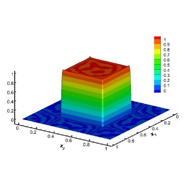
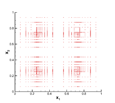
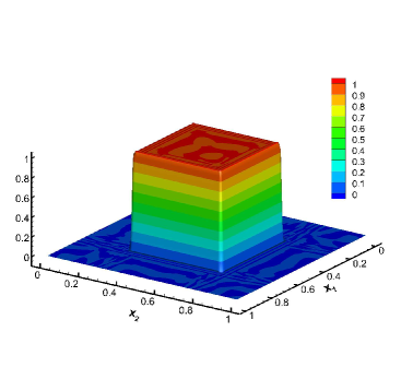
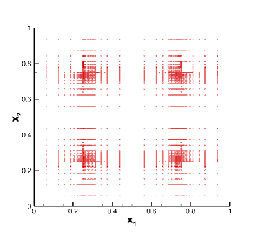
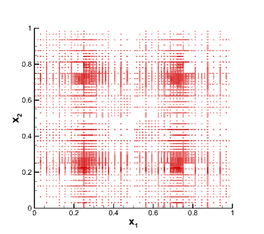
Fig. 1: Example 3.1 with initial condition (19). (a) Numerical solution with $L^{1}$ norm based criteria. (b) Active elements with $L^{1}$ norm based criteria. (c) Numerical solution with $L^{2}$ norm based criteria. (d) Active elements with $L^{2}$ norm based criteria. (e) Numerical solution with $L^{\infty}$ norm based criteria. (f) Active elements with $L^{\infty}$ norm based criteria. $T=1$. $d=2$. $N=7$. $k=3$. $\varepsilon=10^{-5}$.

We then perform a detailed comparison for smooth and non smooth solution to demonstrate an important property of the proposed scheme. We fix $d=2$, $N=7$, $k=3$ and consider initial conditions (18) and (19). We take $\varepsilon=10^{-7}$ and $\varepsilon=10^{-5}$ for the smooth and discontinuous problems, respectively. In Figure 2, we plot the percentage of active elements for each incremental space $\mathbf{W}_{\mathbf{l}}$, $\mathbf{l}={l_{1},l_{2}}$ at final time $T=1$ with all three norms as adaptive indicators. If the percentage is $1,$ it means all the elements on that level is enacted. If the percentage is $0,$ it means no element on that level is enacted. A full grid approximation corresponds to percentage being $1$ on all levels, while a sparse grid approximation [27] corresponds to percentage being $1$ when $|\mathbf{l}|_{1}\leq N,$ and $0$ otherwise. For the adaptive scheme, there is no longer a clean cutoff and we visualize the variation of percentages among all levels when $L^{1}$, $L^{2}$ and $L^{\infty}$ norm based criteria are used. We observe from Figure 2 that only the upper left corner of incremental spaces are active, similar to the sparse grid DG method with space approximation $\hat{{\bf V}}_{N}^{k}$ when the solution is smooth. This is true for all refinement/coarsening criteria. If the solution is discontinuous, more elements are incorporated to fully resolve the discontinuities. The $L^{1}$ norm based criteria is the most sparse among the three as expected. From this plot, we can conclude that if the solution is globally smooth, then the scheme will go back to a sparse grid DG method proposed in [27], leading to great savings in computational cost; otherwise, the adaptive algorithm will automatically use more elements in the refined levels to capture local fine structures.

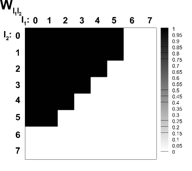
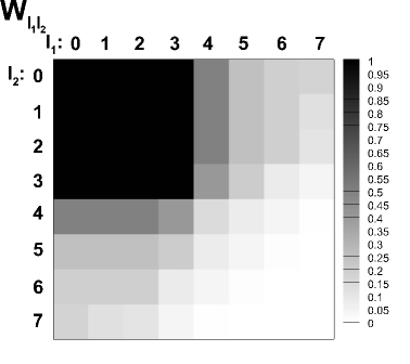
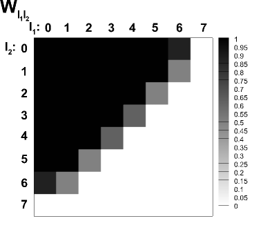
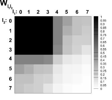
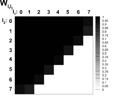
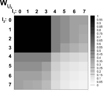
Fig. 2: Example 3.1. The percentage of active elements for each incremental space $\mathbf{W}_{\mathbf{l}}$, $\mathbf{l}=\{l_{1},l_{2}\}$ and $|\mathbf{l}|_{\infty}\leq N$ at final time. $T=1$. $N=7$. $k=3$. $\varepsilon=10^{-7}$ and $\varepsilon=10^{-5}$ for the smooth (a, c, e) and discontinuous (b, d, f) initial conditions, respectively. We use $L^{1}$ norm based criteria (a, b), $L^{2}$ norm based criteria (c, d), and $L^{\infty}$ norm based criteria (e, f).

An additional point we are concerned with is the long time performance of the scheme. For the smooth initial condition (18), we set $T=60,d=4,N=7,k=3$ and keep track of the time evolution of $L^{2}$ errors and the numbers of active degrees of freedom with $\varepsilon=10^{-4},\,10^{-5},\,10^{-6}$ along time evolution as shown in Figure 3. It is observed that, for this linear transport problem, the active degrees of freedom decrease at the very beginning of the simulations, then they nearly remain constant as time evolves for all $\varepsilon$. This is because the profile of solution does not change over time and it is only advected along the characteristic direction. The $L^{2}$ error demonstrates sub-linear growth beyond the initial stage. The maximum $L^{2}$ errors over time are reported in the figure. For the discontinuous initial condition (19), we set $T=10,d=2,N=7,k=3,\varepsilon=10^{-5}$ and report the time evolution the numbers of active degrees of freedom and $L^{1}$ errors in Figure 4 with all three norm based criteria. The scheme with the $L^{\infty}$ norm based criteria yields the smallest error but also involves the largest number of degrees of freedom. The error performance of the $L^{2}$ norm based criteria is qualitatively the same as the $L^{\infty}$ norm based criteria, while much less degrees of freedom are used. The $L^{1}$ norm based criteria leads to the largest error while it is uses the least amount of elements among the three. The maximum $L^{1}$ errors over time are reported in the figure.

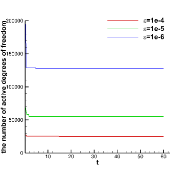
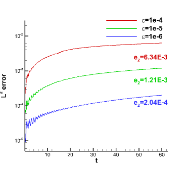
Fig. 3: Example 3.1 with initial condition (18) and $L^{2}$ norm based criteria. (a) Time histories of the number of active degrees of freedom. (b) Time histories of $L^{2}$ errors. $T=60$. $d=4$. $N=7$. $k=3$.

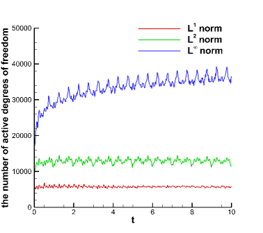
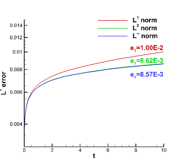
Fig. 4: Example 3.1 with initial condition (19). (a) Time histories of the number of active degrees of freedom. (b) Time histories of $L^{1}$ errors. $T=10$. $d=2$. $N=7$. $k=3$. $\varepsilon=10^{-5}$.

Example 3.2 (Solid body rotation).

We consider solid body rotation, which is in the form of (8) with

$${\bm{a}}=\left(-x_{2}+\frac{1}{2},x_{1}-\frac{1}{2}\right),\quad\text{when}\quad d=2,$$

$${\bm{a}}=\left(-\frac{\sqrt{2}}{2}\left(x_{2}-\frac{1}{2}\right),\frac{\sqrt{2}}{2}\left(x_{1}-\frac{1}{2}\right)+\frac{\sqrt{2}}{2}\left(x_{3}-\frac{1}{2}\right),-\frac{\sqrt{2}}{2}\left(x_{2}-\frac{1}{2}\right)\right),\quad\text{when}\quad d=3,$$

subject to periodic boundary conditions.

This benchmark test is used to assess the performance of the sparse grid DG transport schemes [27]. The initial condition is set to be the following smooth cosine bells (with $C^{5}$ smoothness),

$$u(0,\mathbf{x})=\left\{\begin{array}[]{ll}b^{d-1}\cos^{6}\left(\frac{\pi r}{2b}\right),&\text{if}\quad r\leq b,\\ 0,&\text{otherwise},\end{array}\right.$$ (20)

where $b=0.23$ when $d=2$ and $b=0.45$ when $d=3$, and $r=|\mathbf{x}-\mathbf{x}_{c}|$ denotes the distance between $\mathbf{x}$ and the center of the cosine bell with $\mathbf{x}_{c}=(0.75,0.5)$ for $d=2$ and $\mathbf{x}_{c}=(0.5,0.55,0.5)$ for $d=3.$ As time evolves, the cosine bell traverses along circular trajectories centered at $(1/2,1/2)$ for $d=2$ and about the axis $\{x_{1}=x_{3}\}\cap\{x_{2}=1/2\}$ for $d=3$ without deformation. We start with the investigation of the convergence rate of the adaptive scheme. Similar to the previous example, we run the simulation up to $T=1$ with different $\varepsilon$ and summarize the $L^{2}$ errors, the number of active degrees of freedom and corresponding convergence rates $R_{\varepsilon}$ and $R_{\text{DOF}}$ in Table 2. The maximum mesh level is set as $N=7$. For both $d=2,\,3$, it is observed that the rate $R_{\varepsilon}$ is slightly less than 1 and $R_{\text{DOF}}$ is larger than $\frac{k+1}{d}$ but smaller than $k+1$, which is similar to the previous example.

Table 2: Example 3.2 with initial condition (20). Numerical error and convergence rate. $N=7$. $T=1$.

$\varepsilon$	DOF	$L^{2}$ error	$R_{\text{DOF}}$	$R_{\varepsilon}$	DOF	$L^{2}$ error	$R_{\text{DOF}}$	$R_{\varepsilon}$
	$k=1$, $d=2$				$k=1$, $d=3$
5E-04	260	6.71E-03			928	2.17E-03
1E-04	604	1.53E-03	1.76	0.92	3280	6.32E-04	0.98	1.78
5E-05	764	8.07E-04	2.72	0.92	4912	4.34E-04	0.93	0.24
1E-05	1832	2.37E-04	1.40	0.76	12744	1.14E-04	1.40	1.93
5E-06	2332	1.24E-04	2.69	0.94	20416	6.17E-05	1.31	0.38
1E-06	3440	3.71E-05	3.10	0.75	47496	1.99E-05	1.34	1.63
	$k=2$, $d=2$				$k=2$, $d=3$
1E-04	747	7.15E-04			4779	2.28E-04
5E-05	855	4.43E-04	3.54	0.69	6345	1.54E-04	1.38	0.57
1E-05	1908	1.78E-04	1.14	0.57	14418	4.67E-05	1.46	0.74
5E-06	2376	8.55E-05	3.34	1.06	19845	2.35E-05	2.14	0.99
1E-06	4095	1.51E-05	3.18	1.08	37395	9.07E-06	1.50	0.60
5E-07	4914	9.12E-06	2.77	0.73	50355	4.94E-06	2.04	0.88
	$k=3$, $d=2$				$k=3$, $d=3$
5E-06	1952	6.88E-05			16384	1.02E-05
1E-06	3136	1.19E-05	3.70	1.09	29440	3.36E-06	1.90	0.69
5E-07	3696	5.79E-06	4.40	1.04	39616	1.62E-06	2.45	1.05
1E-07	4992	1.53E-06	4.43	0.83	59456	6.23E-07	2.36	0.60
5E-08	6288	6.19E-07	3.92	1.30	80832	3.53E-07	1.84	0.82
1E-08	9184	1.44E-07	3.85	0.91	129088	2.62E-08	5.56	1.62

We also use this example to compare the performance of the scheme with different configurations of $N$ and $\varepsilon$. We let $d=2$, $k=2$ and compute the solutions up to ten periods and plot the time evolution of $L^{2}$ errors and the number of active degrees of freedom in Figure 5. In particular, we compare maximum mesh level $N=5$ and $N=7,$ and run the simulations with three different values of $\varepsilon$. Since the cosine bell keeps its initial profile as time evolves, the degrees of freedom to resolve the solution for a fixed accuracy threshold should remain the same. We observe that if an excessively small $\varepsilon$ is taken, the used degrees of freedom will increase, but the error may not decrease much, see Figure 5 (a-b). This shows the importance of the choice of $\varepsilon$ and $N$ for the computational efficiency of the scheme.

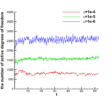
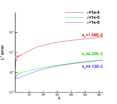
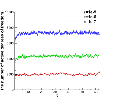
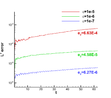
Fig. 5: Example 3.2 with initial condition (20). Time history of the numbers of active degrees of freedom and $L^{2}$ errors with various $\varepsilon$. $k=2$. (a-b) $N=5$. (c-d) $N=7$.

We then consider following discontinuous initial condition:

$$u(0,\mathbf{x})=\left\{\begin{array}[]{ll}\displaystyle 1&(x_{1},x_{2})\in[\frac{3}{4}-\frac{\sqrt{2}}{10},\frac{3}{4}+\frac{\sqrt{2}}{10}]\times[\frac{1}{2}-\frac{\sqrt{2}}{10},\frac{1}{2}+\frac{\sqrt{2}}{10}],\\[5.69054pt] 0&\text{otherwise},\end{array}\right.$$ (21)

when $d=2.$ In the simulation, we set $N=7$, $k=3$, $\varepsilon=10^{-5}$ and consider both $L^{1}$ and $L^{2}$ norm based criteria. In Figure 6, we report the numerical solutions and the associated active elements at $T=2\pi$. Similar to the previous example, elements clusters towards the discontinuities and the scheme with both criteria is able to well resolve the discontinuities. However, more severe localized numerical oscillations are observed when compared with the previous example.

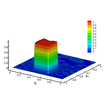
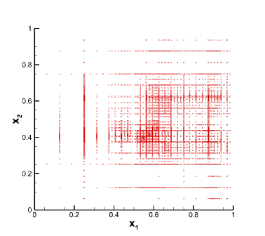
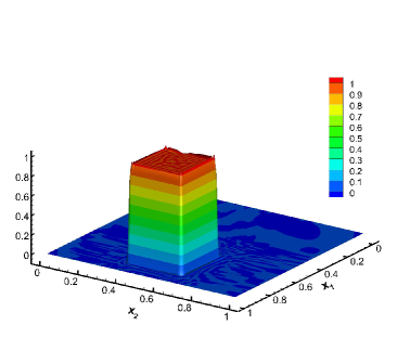
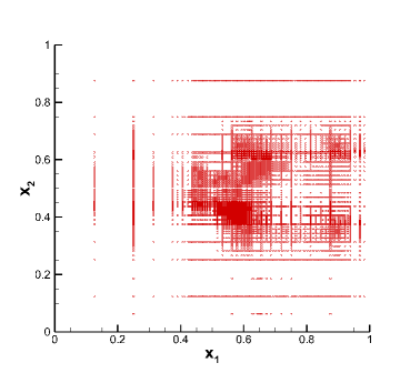
Fig. 6: Example 3.2 with initial condition (21). (a) Numerical solution with $L^{1}$ norm based criteria. (b) Active elements with $L^{1}$ norm based criteria. (c) Numerical solution with $L^{2}$ norm based criteria. (d) Active elements with $L^{2}$ norm based criteria. $T=2\pi$. $d=2$. $N=7$. $k=3$. $\varepsilon=10^{-5}$.

Example 3.3 (Deformational flow).

We consider two-dimensional deformational flow with velocity field

$${\bm{a}}=(\sin^{2}(\pi x_{1})\sin(2\pi x_{2})g(t),-\sin^{2}(\pi x_{2})\sin(2\pi x_{1})g(t)),$$

where $g(t)=\cos(\pi t/T)$ with $T=1.5$.

First, we choose the cosine bell (20) as the initial condition, but with $\mathbf{x}_{c}=(0.65,0.5)$ and $b=0.35$. The cosine bell deforms into a crescent shape at $t=T/2$, then goes back to its initial state at $t=T$ as the flow reverses. We perform a similar convergence study as in the previous two examples, which is summarized in Table 3. We observe similar convergence pattern that the rate $R_{\text{DOF}}$ is slightly smaller than $k+1$ and $R_{\varepsilon}$ is close to 1.

Table 3: Example 3.3 with initial condition (20). Numerical error and convergence rate. $N=7$. $T=1.5$. $d=2$.

$\varepsilon$	DOF	$L^{2}$ error	$R_{\text{DOF}}$	$R_{\varepsilon}$
	$k=1$
1E-03	244	1.52E-02
5E-04	372	7.94E-03	1.53	0.93
1E-04	945	1.25E-03	1.98	1.15
5E-05	1248	1.00E-03	8.01	0.32
1E-05	2608	1.84E-04	2.30	1.05
5E-06	3508	9.96E-05	2.07	0.89
1E-06	5596	3.81E-05	2.06	0.60
	$k=2$
5E-05	1143	5.41E-04
1E-05	2043	1.15E-04	2.67	0.96
5E-06	2736	6.91E-05	1.74	0.73
1E-06	4842	1.24E-05	3.00	1.07
5E-07	5994	8.29E-06	1.90	0.59
1E-07	9045	1.74E-06	3.79	0.97
5E-08	11142	1.08E-06	2.28	0.69
	$k=3$
5E-05	1056	3.65E-04
1E-05	2048	8.85E-05	2.14	0.88
5E-06	2320	5.41E-05	3.94	0.71
1E-06	3904	1.45E-05	2.53	0.82
5E-07	4480	6.32E-06	6.02	1.20
1E-07	6224	1.30E-06	4.80	0.98
5E-08	7680	5.84E-07	3.82	1.16

In Figure 7, we present the contour plots and the associated active elements of the numerical solutions computed with $N=7,\,k=3,\,\varepsilon=10^{-7}$ at $t=T/2$ when the shape of the bell is severely deformed, and $t=T$ when the solution is recovered into its initial state. The elements tend to cluster where the solution deforms as expected, and the shape of the cosine bell is well recovered at $t=T.$

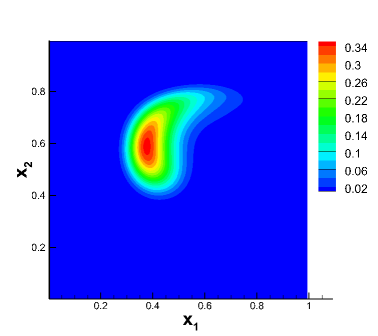
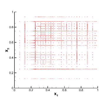
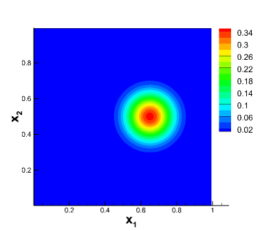
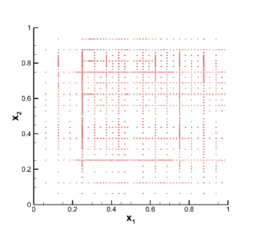
Fig. 7: Example 3.3 with initial condition (20). $N=7$. $k=3$. $\varepsilon=10^{-7}$. (a-b) $t=T/2$. (c-d) $t=T.$

We also consider the discontinuous initial condition (21), and use both $L^{1}$ and $L^{2}$ based refinement/coarsening criteria with $N=7$, $k=3$ and $\varepsilon=10^{-5}$. The numerical solutions and the associated active elements at $t=T/2$ and $t=T$ are plotted in Figures 8 and 9, respectively. For this challenging test, the numerical solution tends to be more oscillatory, again because no limiting mechanism is present in the scheme. The $L^{2}$ norm based criteria generate less oscillatory profiles but use more elements for computation.

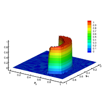
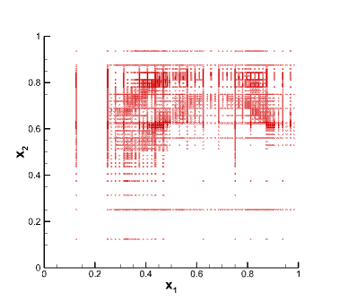
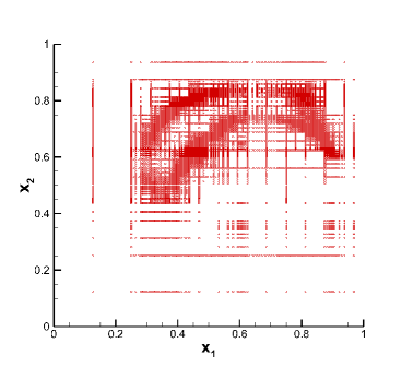
Fig. 8: Example 3.3 with initial condition (21). $t=T/2$. $N=7$. $k=3$. $\varepsilon=10^{-5}$. (a-b) $L^{1}$ norm based criteria. (c-d) $L^{2}$ norm based criteria.

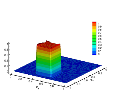
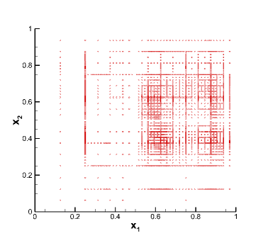
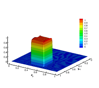
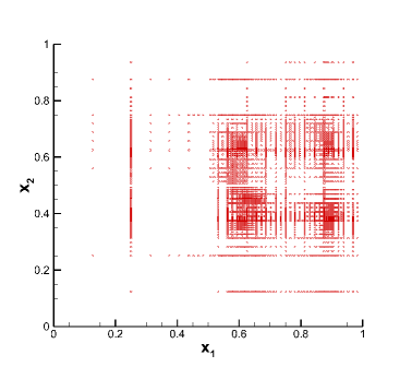
Fig. 9: Example 3.3 with initial condition (21). $t=T$. $N=7$. $k=3$. $\varepsilon=10^{-5}$. (a-b) $L^{1}$ norm based criteria. (c-d) $L^{2}$ norm based criteria.

4 Vlasov-Poisson simulations

In this section, we apply the adaptive multiresolution DG methods to solve the kinetic transport equation. Here, we consider the VP system, which is a fundamental model in plasma simulation. The solution is known to develop filamentation (fine structures) in the phase space. Therefore, it is a good test problem for the adaptive algorithm. For simplicity, we restrict our attention to two dimensional cases, but comment that the algorithm can be readily generalized to higher dimensions and other types of kinetic models.

Example 4.1.

We first consider the non-dimensionalized single-species nonlinear VP system for plasma simulations in the zero-magnetic limit

$$f_{t}+{\bf v}\cdot\nabla_{\mathbf{x}}f+\mathbf{E}(t,\mathbf{x})\cdot\nabla_{\bf v}f=0,$$ (22)

$$-\Delta_{\mathbf{x}}\Phi(\mathbf{x})=\rho-1,\quad\mathbf{E}(\mathbf{x})=-\nabla_{\mathbf{x}}\Phi$$ (23)

where $f(t,\mathbf{x},{\bf v})$ denotes the probability distribution function of electrons. $\mathbf{E}(t,\mathbf{x})$ is the self-consistent electrostatic field given by Poisson’s equation(23) and $\rho(t,\mathbf{x})=\int_{{\bf v}}f(t,\mathbf{x},{\bf v})d{\bf v}$ denotes the electron density. Ions are assumed to form a neutralizing background.

Periodic boundary condition is imposed in $x$-space. As a standard practice, the computational domain in $v$ is truncated to $[-V_{c},V_{c}]$, where $V_{c}$ is a constant chosen large enough to impose zero boundary condition in the $v$-direction $f_{h}(t,x,\pm V_{c})=0.$ The following set of initial conditions will be considered as classical benchmark numerical tests.

• Landau damping:

  $$f(0,x,v)=f_{M}(v)(1+A\cos(kx)),\quad x\in[0,L],\,v\in[-V_{c},V_{c}],$$ (24)

  where $A=0.5$, $k=0.5$, $L=4\pi$, $V_{c}=2\pi$, and $f_{M}(v)=\frac{1}{\sqrt{2\pi}}e^{-v^{2}/2}$.

• Bump-on-tail instability:

  $$f(0,x,v)=f_{BT}(v)(1+A\cos(kx)),\quad x\in[0,L],\,v\in[-V_{c},V_{c}],$$ (25)

  where $A=0.04$, $k=0.3$, $L=20\pi/3$, $V_{c}=13$, and

  $$f_{BT}(v)=n_{p}\exp\left(-\frac{v^{2}}{2}\right)+n_{b}\exp\left(-\frac{|v-u|^{2}}{2v_{t}^{2}}\right),$$

  where $n_{p}=\frac{9}{10\sqrt{10\pi}},\,n_{b}=\frac{2}{10\sqrt{10\pi}},\,u=4.5,\,v_{t}=0.5.$

• Two-stream instability I:

  $$f(0,x,v)=f_{TSI}(v)(1+A\cos(kx)),\quad x\in[0,L],\,v\in[-V_{c},V_{c}],$$ (26)

  where $A=0.05$, $k=0.5$, $L=4\pi$, $V_{c}=2\pi$, and $f_{TSII}(v)=\frac{1}{\sqrt{2\pi}}v^{2}e^{-v^{2}/2}$.

• Two-stream instability II:

  $$f(0,x,v)=f_{TSII}(v)(1+A\cos(kx)),\quad x\in[0,L],\,v\in[-V_{c},V_{c}],$$ (27)

  where $A=0.05$, $k=2/13$, $L=13\pi$, $V_{c}=5$, and

  $$f_{TSII}(v)=\frac{1}{2v_{t}\sqrt{2\pi}}\left(\exp\left(-\frac{|u+v|^{2}}{2v_{t}^{2}}\right)+\exp\left(-\frac{|u-v|^{2}}{2v_{t}^{2}}\right)\right),$$

  where $u=0.99,\,v_{t}=0.3.$

In the literature, RKDG schemes for the VP system [6, 30, 14] have been extensively studied. They are shown to have superior performance in conservation. Our previous work on sparse grid DG method [27] focused on the closely related Vlasov-Ampère (VA) system. The solver in [27] successfully reduced the DOFs of the equations while maintaining key conservation properties. However, when $t$ gets large and filamentation becomes severe, the sparse grid method has difficulties resolving the fine structures in the phase space. It is therefore to our interest to investigate if the adaptive multiresolution scheme can achieve a good balance between computational cost and numerical resolution.

We apply the adaptive algorithm to the Vlasov equation as outlined in Section 2. The Poisson equation is solved by a standard local DG method [5] on the finest level mesh in the $x$-direction. In the simulations, we use $N=7$, $\varepsilon=10^{-5}$ and $k=3$. First we investigate the conservative properties of the scheme. The VP system is known to preserve many physical invariants, including the particle number $\int_{\mathbf{x}}\int_{\bf v}f(t,\mathbf{x},{\bf v})\,d\mathbf{x}d{\bf v},$ momentum $\int_{\mathbf{x}}\int_{\bf v}{\bf v}f(t,\mathbf{x},{\bf v})\,d\mathbf{x}d{\bf v},$ enstrophy $\int_{\mathbf{x}}\int_{\bf v}|f(t,\mathbf{x},{\bf v})|^{2}\,d\mathbf{x}d{\bf v},$ and total energy $\frac{1}{2}\int_{\mathbf{x}}\int_{\bf v}f(t,\mathbf{x},{\bf v})|{\bf v}|^{2}\,d\mathbf{x}d{\bf v}+\frac{1}{2}\int_{\mathbf{x}}|\mathbf{E}(t,\mathbf{x})|^{2}\,d\mathbf{x}.$ Generally speaking, it is difficult for a numerical method to preserve all those invariants. By careful design, DG methods have been designed to preserve the particle number and the energy of the system [6, 13]. For our scheme, in Figure 10, we report the time evolution of the relative errors in total particle number, total energy, enstrophy, and evolution of error in momentum. It is observed that the total particle number is conserved up to the magnitude of $\varepsilon$. This is not as well conserved as a traditional RKDG method. However, it is expected because the adaptive algorithm only keeps elements above the error threshold in the hash table and causing the truncation errors at the velocity boundary to be on the same magnitude of $\varepsilon$, contributing to the numerical errors in particle numbers. However, we do comment that the addition and removal of elements other than level $\mathbf{l}=\mathbf{0}$ in the refinement and coarsening steps will not change the numerical mass because the basis functions are orthogonal. Similarly, the total energy and momentum also show visible and slightly larger errors than the standard RKDG method. The enstrophy exhibits the most visible decay because of the choice of upwind numerical flux.

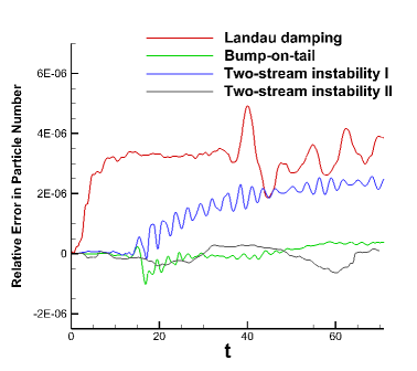
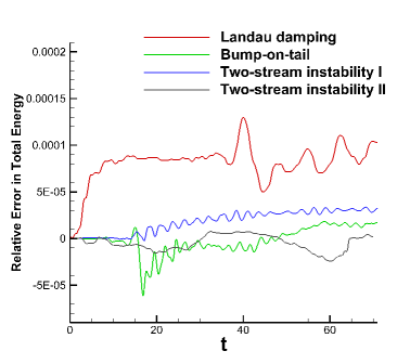
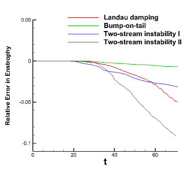
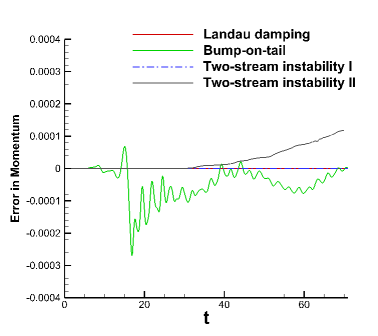
Fig. 10: Example 4.1. Evolution of the relative errors in total particle number (a), total energy (b), enstrophy (c), and evolution of error in momentum (d) with the indicated initial conditions. $N=7$. $k=3$. $\varepsilon=10^{-5}$.

In Figures 11-14, we present the phase space contour plots and the associated active elements at several instances of time for all four initial conditions. In Figure 15, the time evolution of the numbers of active degrees of freedom are plotted. It is observed that when the solution has not developed rich filamentation structures, only a small amount of degrees of freedom are used. As time evolves, thiner and thiner filaments are generated because of phase mixing. The adaptive scheme can automatically add degrees of freedom to adequately resolve the fine structures. We remark that the quality of the numerical results are quite comparable to those computed by the more expensive full grid DG method with similar mesh size, e.g., see [14], while much less degrees of freedom are needed, leading to computational savings.

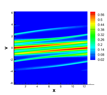
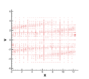
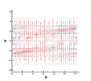
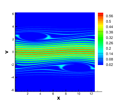
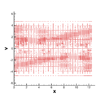
Fig. 11: Example 4.1. Landau damping. Phase space contour plots and the associated active elements at $t=10$ (a-b), $t=20$ (c-d), $t=40$ (e-f). $N=7$. $k=3$. $\varepsilon=10^{-5}$.

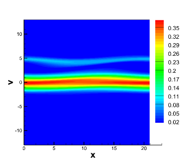
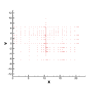
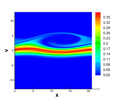
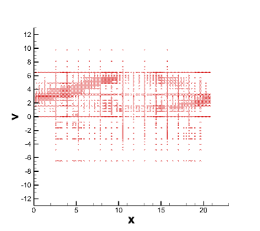
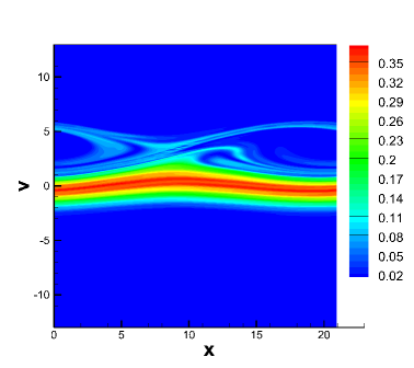
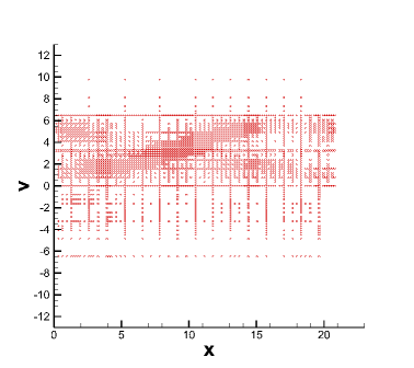
Fig. 12: Example 4.1. Bump-on-tail instability. Phase space contour plots and the associated active elements at $t=10$ (a-b), $t=20$ (c-d), $t=40$ (e-f). $N=7$. $k=3$. $\varepsilon=10^{-5}$.

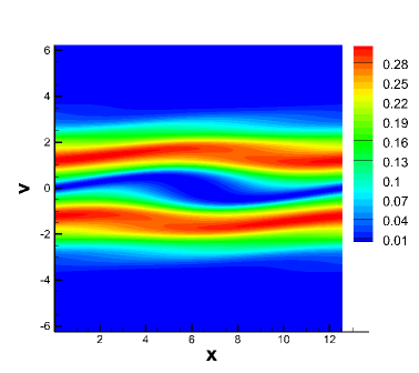
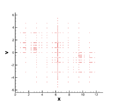
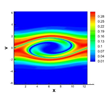
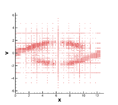
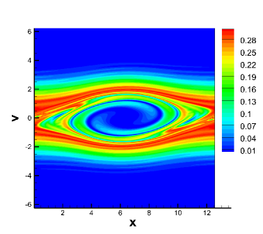
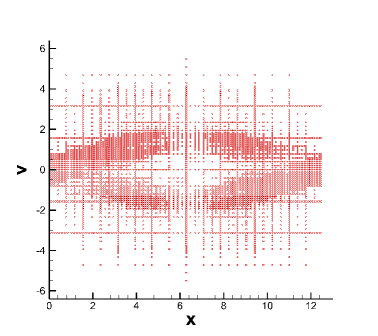
Fig. 13: Example 4.1. Two-stream instability I. Phase space contour plots and the associated active elements at $t=10$ (a-b), $t=20$ (c-d), $t=40$ (e-f). $N=7$. $k=3$. $\varepsilon=10^{-5}$.

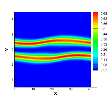
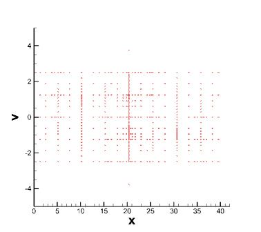
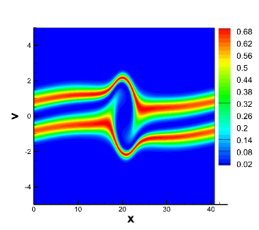
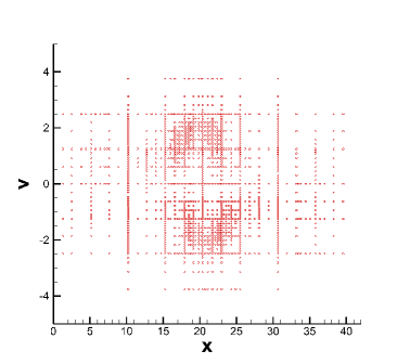
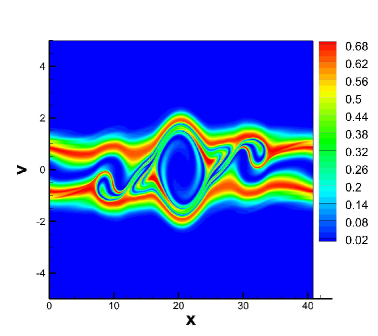
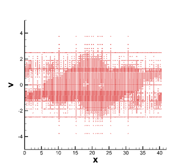
Fig. 14: Example 4.1. Two-stream instability II. Phase space contour plots and the associated active elements at $t=10$ (a-b), $t=20$ (c-d), $t=40$ (e-f). $N=7$. $k=3$. $\varepsilon=10^{-5}$.

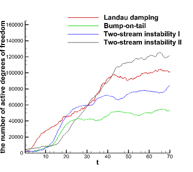
Fig. 15: Example 4.1. Time histories of the number of active degrees of freedom for Landau damping, bump-on-tail, and two types of two-stream instabilities. $k=3$. $N=7$. $\varepsilon=10^{-5}$.

Lastly, we present a numerical comparison between the sparse grid DG method [27] and the adaptive scheme in this paper. We consider two-stream instability I with parameter choice $N=7$, $k=3$ for both methods solving the VP system. The phase space contour plots of the sparse grid DG method at $t=10$ when the solution is very smooth and at $t=20$ when the solution has developed filamentations are provided in Figure 16, to be compared with the results of the adaptive scheme in Figure 13. In Figure 17, we plot the percentage of used elements for each incremental space $\mathbf{W}_{\mathbf{l}}$ at at time $t=10$ and $20$ for the adaptive method. While both schemes actually provide similar accurate description of the macroscopic moments, there is a qualitative difference when the numerical resolution of $f$ is concerned. As expected, when the solution is smooth at $t=10$, both the sparse grid DG method and the adaptive method can generate reliable results with comparable degrees of freedom, see Figure 13(a) and Figure 17(a). At $t=20$, the sparse grid DG method does not resolve all the fine structures when compared with the adaptive method (see Figure 13(c) versus Figure 16(b)). At this time, the adaptive method uses more degrees of freedom than the sparse grid method (see Figure 17(b)), but the DOFs are still much less than the full grid method.

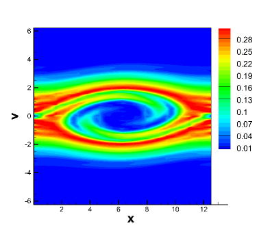
Fig. 16: Example 4.1. Two-stream instability I. Phase space contour plots of the numerical solution by the sparse grid DG scheme [27]. $N=7$. $k=3$. (a) $t=10$. (b) $t=20$.

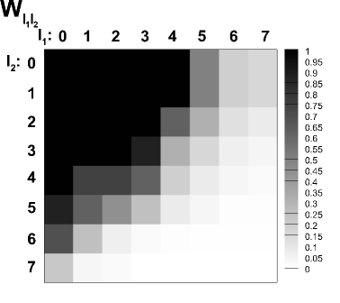
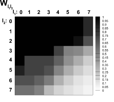
Fig. 17: Example 4.1. Two-stream instability I. The percentage of used elements for each incremental space $\mathbf{W}_{\mathbf{l}}$, $\mathbf{l}=\{l_{1},l_{2}\}$ and $|\mathbf{l}|_{\infty}\leq N$. $N=7$. $k=3$. $\varepsilon=10^{-5}$. (a) $t=10$. (b) $t=20$.

Example 4.2 (Oscillatory VP system).

We consider the following oscillatory VP system in the polar coordinates:

$$f_{t}+\frac{v}{\epsilon}f_{r}+(E(t,r)+E_{ext}(t,r))f_{v}=0,$$ (28)

$$\partial_{r}(rE(t,r))=r\rho(t,r),$$ (29)

where the dimensionless parameter $\epsilon=0.05$ denotes the ratio between the characteristic lengths in the transverse and the longitudinal directions [19]. $E_{ext}$ is the external electric field specified as

$$E_{ext}(t,r)=-\frac{r}{\epsilon}+r\cos^{2}\left(\frac{t}{\epsilon}\right).$$

The initial condition is set to be a discontinuous function

$$f(0,r,v)=\frac{n_{0}}{v_{t}\sqrt{2\pi}}\exp\left(-\frac{v^{2}}{2v_{t}^{2}}\right)\chi_{[-r_{m},r_{m}]}(r),\quad(r,v)\in[-3,3]^{2},$$ (30)

where $n_{0}=4$,  $v_{t}=0.1,\,r_{m}=1.85,$ and

$$\chi_{[-r_{m},r_{m}]}(r)=\left\{\begin{array}[]{ll}1&\text{if}\quad-r_{m}\leq r\leq r_{m},\\ 0&\text{otherwise}.\end{array}\right.$$

This example has been intensively studied in [18, 22, 19], where several effective schemes have been developed. Note that the initial condition (30) considered here is discontinuous and represents a semi-Gaussian beam in particle accelerator physics [19]. We impose zero boundary conditions in both $r$ and $v$ directions. An LDG method is used to solve Poisson’s equation (29) and the closure condition $E(0)=0$ is strongly imposed in the formulation. In the simulation, we let $\epsilon=0.05$, and $k=2$, $N=7$, $\varepsilon=10^{-4}$. We consider both $L^{1}$ ((5) (14)) and $L^{2}$ ((6) (15)) norm based criteria as the refining and coarsening indicators.

We first present the time evolution of the relative errors in total particle number and enstrophy in Figure 18. Similar to the previous VP system, the scheme with both adaptive indicators is able to conserve the particle number up to the magnitude of $\varepsilon$. The enstrophy decays due to the choice of the numerical flux.

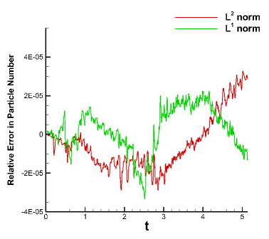
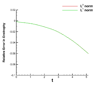
Fig. 18: Example 4.2. Evolution of the relative errors in total particle number (a), enstrophy (b). $N=7$. $k=2$. $\varepsilon=10^{-4}$.

The phase space contours from our scheme agrees well with those in the literature [19]. In Figure 19, we present the contour plots and the associated active elements at three instances of time, for which the $L^{1}$ norm based criteria are used as the adaptive indicator. In Figure 20, we also report the contour plot and associated adaptive mesh at final time with the $L^{2}$ norm based criteria to compare the performance of the two criteria as adaptive indicators. It is observed that the numerical results are qualitatively the same, but more elements are used by the scheme with the $L^{2}$ norm based criteria. In Figure 18, the time evolution of the number of active degrees of freedom are plotted. Again, when the solution develops filaments, more degrees of freedom are added thanks to the adaptive mechanism. In summary, for this example, the $L^{1}$ norm based criteria is preferred for the sake of efficiency.

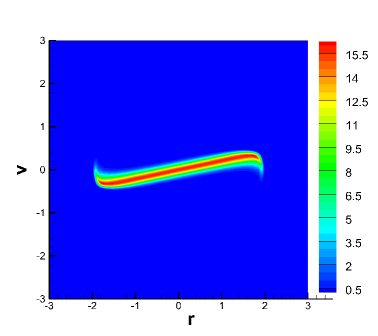
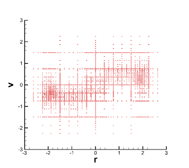
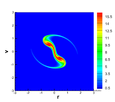
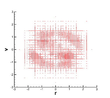
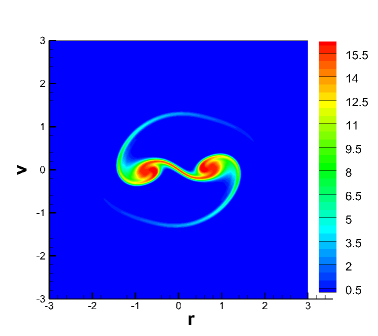
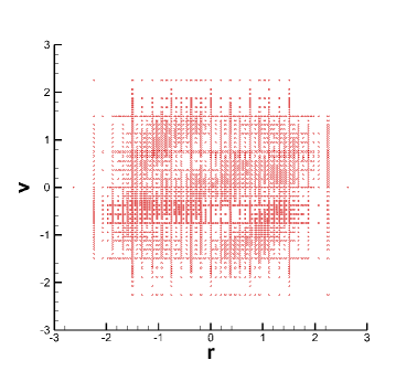
Fig. 19: Example 4.2. Phase space contour plots and the associated active elements at $t=1.3464$ (a-b), $t=4.3388$ (c-d), $t=5.1462$ (e-f). $N=7$. $k=2$. $\varepsilon=10^{-4}$. The $L^{1}$ norm based criteria are used as the adaptive indicator.

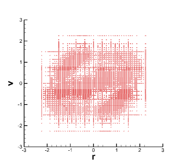
Fig. 20: Example 4.2. Phase space contour plots and the associated active elements at $t=5.1462$. $k=2$. $N=7$. $\varepsilon=10^{-4}$. The $L^{2}$ norm based criteria are used as the adaptive indicator.

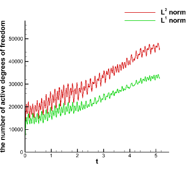
Fig. 21: Example 4.2. Time histories of the number of active degrees of freedom. $N=7$. $k=2$. $\varepsilon=10^{-4}$.

5 Conclusions and future work

In this paper, we develop an adaptive multiresolution DG scheme for computing time-dependent transport equations. The key ingredients of the scheme are the weak formulation of the DG method and adaptive error thresholding based on hierarchical surplus. Extensive numerical tests show that our scheme performs similarly to a sparse grid DG method when the solution is smooth, and can automatically capture fine local structures when the solution is no longer smooth. Detailed comparison between several refinement/coarsening error indicators are performed. The method is demonstrated to work well for kinetic simulations. Future work consists of the study of limiters and further improvement of the scheme including local time stepping and adaptivity with both the mesh and polynomial degrees.

References

- [1] B. Alpert. A class of bases in 2 for the sparse representation of integral operators. SIAM Journal on Mathematical Analysis, 24(1):246–262, 1993.
- [2] B. Alpert, G. Beylkin, D. Gines, and L. Vozovoi. Adaptive solution of partial differential equations in multiwavelet bases. Journal of Computational Physics, 182(1):149–190, Oct. 2002.
- [3] M. A. Alves, P. Cruz, A. Mendes, F. D. Magalhães, F. T. Pinho, and P. J. Oliveira. Adaptive multiresolution approach for solution of hyperbolic PDEs. Computer Methods in Applied Mechanics and Engineering, 191(36):3909–3928, Aug. 2002.
- [4] R. Archibald, G. Fann, and W. Shelton. Adaptive discontinuous Galerkin methods in multiwavelets bases. Applied Numerical Mathematics, 61(7):879–890, July 2011.
- [5] D. Arnold, F. Brezzi, B. Cockburn, and L. Marini. Unified analysis of discontinuous Galerkin methods for elliptic problems. SIAM J. Numer. Anal., 39:1749–1779, 2002.
- [6] B. Ayuso, J. A. Carrillo, and C.-W. Shu. Discontinuous Galerkin methods for the one-dimensional Vlasov-Poisson system. Kinetic and Related Models, 4:955–989, 2011.
- [7] N. Besse, F. Filbet, M. Gutnic, I. Paun, and E. Sonnendrücker. An adaptive numerical method for the vlasov equation based on a multiresolution analysis. In Numerical Mathematics and Advanced Applications, pages 437–446. Springer, 2003.
- [8] N. Besse, G. Latu, A. Ghizzo, E. Sonnendrücker, and P. Bertrand. A wavelet-MRA-based adaptive semi-Lagrangian method for the relativistic Vlasov–Maxwell system. Journal of Computational Physics, 227(16):7889–7916, Aug. 2008.
- [9] B. Bihari and A. Harten. Multiresolution schemes for the numerical solution of 2-D conservation laws I. SIAM Journal on Scientific Computing, 18(2):315–354, Mar. 1997.
- [10] O. Bokanowski, J. Garcke, M. Griebel, and I. Klompmaker. An adaptive sparse grid Semi-Lagrangian scheme for first order Hamilton-Jacobi Bellman equations. Journal of Scientific Computing, 55(3):575–605, Oct. 2012.
- [11] H.-J. Bungartz and M. Griebel. Sparse grids. Acta numer., 13:147–269, 2004.
- [12] J. L. D. Calle, P. R. B. Devloo, and S. M. Gomes. Wavelets and adaptive grids for the discontinuous Galerkin method. Numerical Algorithms, 39(1-3):143–154, July 2005.
- [13] Y. Cheng, A. J. Christlieb, and X. Zhong. Energy-conserving discontinuous Galerkin methods for the Vlasov–Ampère system. Journal of Computational Physics, 256:630–655, 2014.
- [14] Y. Cheng, I. M. Gamba, and P. J. Morrison. Study of conservation and recurrence of Runge–Kutta discontinuous Galerkin schemes for Vlasov-Poisson systems. Journal of Scientific Computing, 56:319–349, 2013.
- [15] G. Chiavassa, R. Donat, and S. Müller. Multiresolution-based adaptive schemes for hyperbolic conservation laws. In Adaptive Mesh Refinement-Theory and Applications, pages 137–159. Springer, 2005.
- [16] A. Cohen. Wavelet methods in numerical analysis. Handbook of numerical analysis, 7:417–711, 2000.
- [17] A. Cohen, S. Kaber, S. Müller, and M. Postel. Fully adaptive multiresolution finite volume schemes for conservation laws. Mathematics of Computation, 72(241):183–225, 2003.
- [18] N. Crouseilles, M. Lemou, and F. Méhats. Asymptotic Preserving schemes for highly oscillatory Vlasov–Poisson equations. Journal of Computational Physics, 248:287–308, 2013.
- [19] N. Crouseilles, M. Lemou, F. Méhats, and X. Zhao. Uniformly accurate forward semi-Lagrangian methods for highly oscillatory Vlasov-Poisson equations. Inria preprint, hal-01286947, Mar. 2016.
- [20] W. Dahmen. Wavelet and multiscale methods for operator equations. Acta Numerica, 6:55–228, Jan. 1997.
- [21] W. Dahmen, B. Gottschlich–Müller, and S. Müller. Multiresolution schemes for conservation laws. Numerische Mathematik, 88(3):399–443, May 2001.
- [22] E. Frénod, S. A. Hirstoaga, and E. Sonnendrücker. An exponential integrator for a highly oscillatory Vlasov equation. Discrete and Continuous Dynamical Systems - Series S, 8(1):169–183, 2015.
- [23] J. Garcke and M. Griebel. Sparse grids and applications. Springer, 2013.
- [24] N. Gerhard, F. Iacono, G. May, S. Müller, and R. Schäfer. A high-order discontinuous Galerkin discretization with multiwavelet-based grid adaptation for compressible flows. Journal of Scientific Computing, 62(1):25–52, Mar. 2014.
- [25] N. Gerhard and S. Müller. Adaptive multiresolution discontinuous Galerkin schemes for conservation laws: multi-dimensional case. Computational and Applied Mathematics, pages 1–29, Apr. 2014.
- [26] M. Griebel. Adaptive sparse grid multilevel methods for elliptic PDEs based on finite differences. Computing, 61(2):151–179, 1998.
- [27] W. Guo and Y. Cheng. A sparse grid discontinuous galerkin method for high-dimensional transport equations and its application to kinetic simulations. arXiv preprint arXiv:1602.02124, 2016. SISC under review.
- [28] M. Gutnic, M. Haefele, I. Paun, and E. Sonnendrücker. Vlasov simulations on an adaptive phase-space grid. Computer Physics Communications, 164(1–3):214–219, Dec. 2004.
- [29] A. Harten. Multiresolution algorithms for the numerical solution of hyperbolic conservation laws. Communications on Pure and Applied Mathematics, 48(12):1305–1342, Dec. 1995.
- [30] R. Heath, I. Gamba, P. Morrison, and C. Michler. A discontinuous Galerkin method for the Vlasov-Poisson system. Journal of Computational Physics, 231(4):1140–1174, 2012.
- [31] N. Hovhannisyan, S. Müller, and R. Schäfer. Adaptive multiresolution discontinuous Galerkin schemes for conservation laws. Mathematics of Computation, 83(285):113–151, 2014.
- [32] F. Iacono, G. May, S. Müller, and R. Schäfer. An Adaptive Multiwavelet-Based DG Discretization for Compressible Fluid Flow. In A. Kuzmin, editor, Computational Fluid Dynamics 2010: Proceedings of the Sixth International Conference on Computational Fluid Dynamics, ICCFD6, St Petersburg, Russia, on July 12-16, 2010, pages 813–820. Springer Berlin Heidelberg, Berlin, Heidelberg, 2011.
- [33] C.-W. Shu and S. Osher. Efficient implementation of essentially non-oscillatory shock-capturing schemes. J. Comput. Phys., 77:439–471, 1988.
- [34] Z. Wang, Q. Tang, W. Guo, and Y. Cheng. Sparse grid discontinuous Galerkin methods for high-dimensional elliptic equations. J. Comput. Phys., 314:244—263, 2016.
- [35] C. Zenger. Sparse grids. In Parallel Algorithms for Partial Differential Equations, Proceedings of the Sixth GAMM-Seminar, volume 31, 1990.
- [36] H. Zhu and J.-M. Qiu. An -adaptive rkdg method for the vlasov-poisson system. J Sci Comput, 2016.