Solving finite-domain linear constraints in presence of the alldifferent

Abstract.

In this paper, we investigate the possibility of improvement of the widely-used filtering algorithm for the linear constraints in constraint satisfaction problems in the presence of the alldifferent constraints. In many cases, the fact that the variables in a linear constraint are also constrained by some alldifferent constraints may help us to calculate stronger bounds of the variables, leading to a stronger constraint propagation. We propose an improved filtering algorithm that targets such cases. We provide a detailed description of the proposed algorithm and prove its correctness. We evaluate the approach on five different problems that involve combinations of the linear and the alldifferent constraints. We also compare our algorithm to other relevant approaches. The experimental results show a great potential of the proposed improvement.

1. Introduction

A constraint satisfaction problem (CSP) over a finite set of variables is the problem of finding values for the variables from their finite domains such that all the imposed constraints are satisfied. There are many practical problems that can be expressed as CSPs, varying from puzzle solving, scheduling, combinatorial design problems, and so on. Because of the applicability of CSPs, many different solving techniques have been considered in the past decades. More details about solving CSPs can be found in [csp_handbook].

A special attention in CSP solving is payed to so-called global constraints which usually have their own specific semantics and are best handled by specialized filtering algorithms that remove the values inconsistent with the constraints and trigger the constraint propagation. These filtering algorithms usually consider each global constraint separately, i.e. a filtering algorithm is typically executed on a constraint without any awareness of the existence of other global constraints. In some cases, however, it would be beneficial to take into account the presence of other global constraints in a particular CSP, since this could lead to a stronger propagation. For example, many common problems can be modeled by CSPs that include some combination of the alldifferent constraints (that constrain their variables to take pairwise distinct values) and linear constraints that are relations of the form $a_{1}\cdot x_{1}+\ldots{}+a_{n}\cdot x_{n}\leq c$ ($\leq$ can be replaced by some other relation symbol, such as $\geq$, $=$, etc.). A commonly used filtering algorithm for linear constraints ([stuckey_bounds]) enforces bound consistency on a constraint — for each variable the maximum and/or the minimum are calculated, and the values outside of this interval are pruned (removed) from the domain. The maximum/minimum for a variable is calculated based on the current maximums/minimums of other variables in the constraint. If we knew that some of the variables in the linear constraint were also constrained by some alldifferent constraint to be pairwise distinct, we would potentially be able to calculate stronger bounds, leading to more prunings. Let as consider the following example.

Consider an instance of the well-known Kakuro puzzle (Figure 1). Each empty cell should be filled with a number from $1$ to $9$ such that all numbers in each line (a vertical or horizontal sequence of adjacent empty cells) are pairwise distinct and their sum is equal to the adjacent number given in the grid. The problem is modeled by the CSP where a variable with the domain $\{1,\ldots{},9\}$ is assigned to each empty cell, variables in each line are constrained with an alldifferent constraint and with one linear constraint that constrains the variables to sum up to the given number.

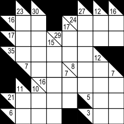
Figure 1. Kakuro puzzle

Consider, for instance, the first horizontal line in the bottom row — it consists of three cells whose values should sum up to $6$. Assume that the variables assigned to these cells are $x$, $y$ and $z$, respectively. These variables are constrained by the constraint $\mathtt{alldifferent}(x,y,z)$ and by the linear constraint $x+y+z=6$. If the filtering algorithm for the linear constraint is completely unaware of the existence of the alldifferent constraint, it will deduce that the values for $x$, $y$ and $z$ must belong to the interval $[1,4]$, since a value greater than $4$ for the variable $x$ together with the minimal possible values for $y$ and $z$ (and that is $1$) sum up to at least $7$ (the symmetric situation is with variables $y$ and $z$). But if the filtering algorithm was aware of the presence of the alldifferent constraint, it would deduce that the feasible interval is $[1,3]$, since the value $4$ for $x$ imposes that the values for $y$ and $z$ must both be $1$, and this is not possible, since $y$ and $z$ must be distinct.

The above example demonstrates the case when a modification of a filtering algorithm that makes it aware of the presence of other constraints imposed on its variables may lead to a stronger propagation. In this paper, we consider this specific case of improving the filtering algorithm for linear constraints in the presence of the alldifferent constraints. The goal of this study is to evaluate the effect of such improvement on the overall solving process. We designed and implemented a simple algorithm that strengthens the calculated bounds based on the alldifferent constraints. The paper also contains the proof of the algorithm’s correctness as well as an experimental evaluation that shows a very good behaviour of our improved algorithm on specific problems that include a lot of alldifferent-constrained linear sums. We must stress that, unlike some other approaches, our algorithm does not establish bound consistency on a conjunction of a linear and an alldifferent constraint, but despite the weaker consistency level, it performs very well in practice. On the other hand, the main advantage of our algorithm is its generality, since it permits arbitrary combinations of the linear and the alldifferent constraints (in particular, the algorithm can handle the combination of a linear constraint with multiple alldifferent constraints that partially overlap with the linear constraint’s variables).

2. Background

A Constraint Satisfaction Problem (CSP) is represented by a triplet $(\mathbf{X},\mathbf{D},\mathbf{C})$, where $\mathbf{X}=(x_{1},x_{2},\ldots{},x_{n})$ is a finite set of variables, $\mathbf{D}=(D_{x_{1}},D_{x_{2}},\ldots{},D_{x_{n}})$ is a set of finite domains, where $D_{x_{i}}$ is the domain of the variable $x_{i}$, $\mathbf{C}=\{C_{1},C_{2},\ldots{},C_{m}\}$ is a finite set of constraints. A constraint $C\in\mathbf{C}$ over variables $x_{i_{1}},x_{i_{2}},\ldots{},x_{i_{k}}$ is some subset of $D_{x_{i_{1}}}\times D_{x_{i_{2}}}\times\ldots{}\times D_{x_{i_{k}}}$. The number $k$ is called arity of the constraint $C$. A solution of CSP is any $n$-tuple $(d_{1},d_{2},\ldots{},d_{n})$ from $D_{x_{1}}\times D_{x_{2}}\times\ldots{}\times D_{x_{n}}$ such that for each constraint $C\in\mathbf{C}$ over variables $x_{i_{1}},x_{i_{2}},\ldots{},x_{i_{k}}$ $k$-tuple $(d_{i_{1}},d_{i_{2}},\ldots{},d_{i_{k}})$ is in $C$. A CSP problem is consistent if it has a solution, and inconsistent otherwise. Two CSP problems $P_{1}$ and $P_{2}$ are equivalent if each solution of $P_{1}$ is also a solution of $P_{2}$ and vice-versa.

A constraint $C$ over variables $x_{i_{1}},x_{i_{2}},\ldots{},x_{i_{k}}$ is hyper-arc consistent if for each value $d_{i_{r}}\in D_{x_{i_{r}}}$ ($r\in\{1,\ldots{},k\}$) there are values $d_{i_{s}}\in D_{x_{i_{s}}}$ for each $s\in\{1,\ldots{},k\}\setminus\{r\}$, such that $(d_{i_{1}},\ldots{},d_{i_{k}})\in C$. Assuming that the domains are ordered, a constraint $C$ over variables $x_{i_{1}},x_{i_{2}},\ldots{},x_{i_{k}}$ is bound consistent if for each value $d_{i_{r}}\in\{min(D_{x_{i_{r}}}),max(D_{x_{i_{r}}})\}$ ($r\in\{1,\ldots{},k\}$) there are values $d_{i_{s}}\in[min(D_{x_{i_{s}}}),max(D_{x_{i_{s}}})]$ for each $s\in\{1,\ldots{},k\}\setminus\{r\}$, such that $(d_{i_{1}},\ldots{},d_{i_{k}})\in C$. A CSP problem is hyper-arc consistent (bound consistent) if all its constraints are.

Constraints whose arity is greater then two are often called global constraints. There are two types of global constraints that are specially interesting for us here. One is the alldifferent constraint defined as follows:

$$\mathtt{alldifferent}(x_{i_{1}},x_{i_{2}},\ldots{},x_{i_{k}})=\{(d_{i_{1}},d_{i_{2}},\ldots{},d_{i_{k}})\ |\ d_{i_{j}}\in D_{x_{i_{j}}},r\neq s\Rightarrow d_{i_{r}}\neq d_{i_{s}}\}$$

The consistency check for the alldifferent constraint is usually reduced to the maximal matching problem in bipartite graphs ([hoeve]). The hyper-arc consistency on an alldifferent constraint can be enforced by Regin’s algorithm ([regin]).

Another type of constraint interesting for us is the linear constraint of the form:

$$a_{1}\cdot x_{1}+\ldots{}+a_{k}\cdot x_{k}\Join c$$

where $\Join\in\{=,\neq,\leq,<,\geq,>\}$, $a_{i}$ and $c$ are integers and $x_{i}$ are finite domain integer variables. Notice that we can assume without lost of generality that the only relations that appear in the problem are $\leq$ and $\geq$. Indeed, a strict inequality $e<c$ ($e>c$) may always be replaced by $e\leq c-1$ ($e\geq c+1$), an equality $e=c$ may be replaced by the conjunction $e\leq c\wedge e\geq c$ and a disequality $e\neq c$ may be replaced by the disjunction $e\leq c-1\vee e\geq c+1$. These replacements can be done in the preprocessing stage. The bound consistency on a linear constraint can be enforced by the filtering algorithm given, for instance, in [stuckey_bounds], and discussed in more details later in the paper.

The CSP solving usually combines search with constraint propagation. By search we mean dividing the problem $P$ into two or more subproblems $P_{1},\ldots{},P_{n}$ such that the solution set of $P$ is the union of the solution sets of the subproblems $P_{1},\ldots{},P_{n}$. The subproblems are then recursively checked for consistency one by one – if any of them is consistent, the problem $P$ is consistent, too. The usual way to split the problem $P$ is to consider different values for some variable $x$. On the other hand, the constraint propagation uses inference to transform the problem $P$ into a simpler but equivalent problem $P^{\prime}$. This is usually done by pruning, i.e. removing the values from the variable domains that are found to be inconsistent with some of the constraints and propagating these value removals to other interested constraints. More detailed information on different search and propagation techniques and algorithms can be found in [csp_handbook].

3. Linear constraints and alldifferent

In this section we consider the improvement of the standard filtering algorithm ([stuckey_bounds]) for the linear constraints which takes into account the presence of the alldifferent constraints. We first briefly explain the standard algorithm, and then we discuss the improved algorithm and prove its correctness.

3.1. Standard filtering algorithm

Assume that we have the linear constraint $e\leq c$, where $e\equiv a_{1}\cdot x_{1}+\ldots{}+a_{n}\cdot x_{n}$. The procedure $\mathtt{calculateBoundsStandard}(e,c,bounds)$ (Algorithm 1) implements the standard filtering algorithm. It receives $e$ and $c$ as inputs and returns $true$ if the constraint $e\leq c$ is consistent, and $false$ otherwise. It also has an output parameter $bounds$ to which it stores the calculated bounds (only if the constraint is consistent). The idea is to first calculate the minimum of the left-hand side expression $e$ (denoted by $min(e)$) in the following way:

$$min(e)=min(a_{1}\cdot x_{1})+\ldots{}+min(a_{n}\cdot x_{n})$$

where

$$\begin{array}[]{ccc}min(a_{i}\cdot x_{i})&=&\left\{\begin{array}[]{cc}a_{i}\cdot min(x_{i}),&a_{i}>0\\ a_{i}\cdot max(x_{i}),&a_{i}<0\\ \end{array}\right.\\ \end{array}$$

If $min(e)>c$, then the constraint is inconsistent. Otherwise, for each variable $x_{i}$ we calculate the minimum of the expression $e_{x_{i}}$ obtained from the expression $e$ by removing the monomial $a_{i}\cdot x_{i}$, that is $e_{x_{i}}\equiv a_{1}\cdot x_{1}+\ldots{}+a_{i-1}\cdot x_{i-1}+a_{i+1}\cdot x_{i+1}+\ldots{}+a_{n}\cdot x_{n}$. Such minimum $min(e_{x_{i}})$ is trivially calculated as $min(e)-min(a_{i}\cdot x_{i})$. Now, for each variable $x_{i}$ we have that:

$$x_{i}\leq\left\lfloor\frac{c-min(e_{x_{i}})}{a_{i}}\right\rfloor\ \mathrm{if}\ a_{i}>0\quad\mathrm{and}\quad x_{i}\geq\left\lceil\frac{c-min(e_{x_{i}})}{a_{i}}\right\rceil\ \mathrm{if}\ a_{i}<0$$ (1)

The values that do not satisfy the calculated bound should be pruned from the domain of the corresponding variable. These prunings ensure that the constraint is bound consistent.

A similar analysis can be done for the constraint $e\geq c$, only then the maximums are considered:

$$max(e)=max(a_{1}\cdot x_{1})+\ldots{}+max(a_{n}\cdot x_{n})$$

where

$$\begin{array}[]{ccc}max(a_{i}\cdot x_{i})&=&\left\{\begin{array}[]{cc}a_{i}\cdot max(x_{i}),&a_{i}>0\\ a_{i}\cdot min(x_{i}),&a_{i}<0\\ \end{array}\right.\\ \end{array}$$

If $max(e)<c$, the constraint is inconsistent. Otherwise, the bounds for the variables are calculated as follows:

$$x_{i}\geq\left\lceil\frac{c-max(e_{x_{i}})}{a_{i}}\right\rceil\ \mathrm{if}\ a_{i}>0\quad\mathrm{and}\quad x_{i}\leq\left\lfloor\frac{c-max(e_{x_{i}})}{a_{i}}\right\rfloor\ \mathrm{if}\ a_{i}<0$$ (2)

0:  $e=a_{1}\cdot x_{1}+\ldots{}+a_{n}\cdot x_{n}$

0:  imposed constraint is $e\leq c$

0:  $bounds[x_{i}]$ holds the calculated bound for $x_{i}$ (upper bound if $a_{i}>0$, lower bound if $a_{i}<0$)

  begin

  {Let $V(e)$ denote the set of variables appearing in $e$}

  {First, we calculate minimum $min(e)$}

  $min(e)=0$

  for all $x_{i}\in V(e)$ do

     if $a_{i}>0$ then

        $min(e)=min(e)+a_{i}\cdot min(x_{i})$

     else

        $min(e)=min(e)+a_{i}\cdot max(x_{i})$

  {Next, we check for inconsistency}

  if $min(e)>c$ then

     return false {inconsistency is detected}

  {Finally, we calculate the bounds of the variables in $V(e)$}

  for all $x_{i}\in V(e)$ do

     if $a_{i}>0$ then

        $min(e_{x_{i}})=min(e)-a_{i}\cdot min(x_{i})$

        $bounds[x_{i}]=\left\lfloor\frac{c-min(e_{x_{i}})}{a_{i}}\right\rfloor$ {upper bound}

     else

        $min(e_{x_{i}})=min(e)-a_{i}\cdot max(x_{i})$

        $bounds[x_{i}]=\left\lceil\frac{c-min(e_{x_{i}})}{a_{i}}\right\rceil$ {lower bound}

  return true {inconsistency is not detected}

  end

Algorithm 1 $\mathtt{calculateBoundsStandard}(e,c,bounds)$

3.2. Improved filtering algorithm

Assume again the constraint $e\leq c$, where $e\equiv a_{1}\cdot x_{1}+\ldots{}+a_{n}\cdot x_{n}$. The goal is to calculate the improved minimum of the expression $e$ (denoted by $min^{*}(e)$), taking into account the imposed alldifferent constraints on variables in $e$. If that improved minimum is greater than $c$, the constraint is inconsistent. Otherwise, we calculate in the similar fashion the improved minimums $min^{*}(e_{x_{i}})$ which are then used to calculate the bounds for the variables (in the similar way as in the standard algorithm):

$$x_{i}\leq\left\lfloor\frac{c-min^{*}(e_{x_{i}})}{a_{i}}\right\rfloor\ \mathrm{if}\ a_{i}>0\quad\mathrm{and}\quad x_{i}\geq\left\lceil\frac{c-min^{*}(e_{x_{i}})}{a_{i}}\right\rceil\ \mathrm{if}\ a_{i}<0$$ (3)

For efficiency, we would like to avoid calculating each $min^{*}(e_{x_{i}})$ from scratch. So there are two main issues to consider here: the first is how to calculate the improved minimum $min^{*}(e)$, and the second is how to efficiently calculate the correction for $min^{*}(e_{x_{i}})$, i.e. the value $c_{i}$ such that $min^{*}(e_{x_{i}})=min^{*}(e)-c_{i}$. The similar situation is with the constraint $e\geq c$, except in that case the improved maximums $max^{*}(e)$ and $max^{*}(e_{x_{i}})$ are calculated, and then the bounds are obtained from the following formulae:

$$x_{i}\geq\left\lceil\frac{c-max^{*}(e_{x_{i}})}{a_{i}}\right\rceil\ \mathrm{if}\ a_{i}>0\ \mathrm{and}\ x_{i}\leq\left\lfloor\frac{c-max^{*}(e_{x_{i}})}{a_{i}}\right\rfloor\ \mathrm{if}\ a_{i}<0$$ (4)

We develop the improved algorithm in two stages. First we consider the simple case where all coefficients $a_{i}$ are of the same sign, and there is the constraint $\texttt{alldifferent}(x_{1},\ldots{},x_{n})$ in the considered problem (i.e. all the variables in $e$ must be pairwise distinct). Then we consider the general case, where there may be more than one alldifferent constraints that (partially) overlap with the variables of $e$, and the coefficients $a_{i}$ may be both positive or negative.

3.2.1. Simple case

Assume that $a_{i}>0$. The improved minimum $min^{*}(e)$ is calculated by the procedure $\mathtt{calculateImprovedMinimum}(e,min,M,p)$ (Algorithm 2). The procedure takes the expression $e$ as its input and calculates the improved minimum of $e$ (returned by the output parameter $min$), the minimizing matching $M$ and the next candidate index vector $p$ (which is later used for calculating corrections). A matching $M$ is a sequence of assignments $[x_{i_{1}}=d_{i_{1}},\ldots{},x_{i_{n}}=d_{i_{n}}]$, where $x_{i_{1}},\ldots{},x_{i_{n}}$ is a permutation of $x_{1},\ldots{},x_{n}$, such that $d_{i_{j}}\geq min(x_{i_{j}})$ (i.e. each variable takes a value greater or equal to its minimum) and $d_{i_{k}}<d_{i_{l}}$ for $k<l$ (i.e. the alldifferent constraint is satisfied). A matching $M$ is minimizing if $\sum_{j=1}^{n}a_{i_{j}}\cdot d_{i_{j}}$ is as minimal as possible. The procedure constructs such matching and assigns the value $\sum_{j=1}^{n}a_{i_{j}}\cdot d_{i_{j}}$ to $min$.

0:  $e=a_{1}\cdot x_{1}+\ldots{}+a_{n}\cdot x_{n}$

0:  $a_{i}>0$

0:  $M=[x_{i_{1}}=d_{i_{1}},\ldots{},x_{i_{n}}=d_{i_{n}}]$ is a minimizing matching

0:  $min=\sum_{j=1}^{n}a_{i_{j}}\cdot d_{i_{j}}$

0:  $p[j]$ is the index in $M$ of the variable which was the next best choice for the value $d_{i_{j}}$, or $undef$ if there were no other candidates

  begin

  {Let $V(e)$ denote the set of variables appearing in $e$}

  $vars=sort(V(e))$ {sort $V(e)$ with respect to the ascending order of minimums}

  $heap.init()$ {$heap$ will contain variables, and the variable with the greatest coefficient will always be on the top of $heap$ (in case of multiple such variables, the one with the smallest index in $e$ will be on the top). Initially, $heap$ is empty}

  $min=0$

  $M=[\ ]$ {Initially, $M$ is an empty sequence}

  $i=1$

  $d=min(vars[1])-1$

  for $j=1$ to $n$ do

     $d=max(d+1,min(vars[j]))$ {calculate the next value to be assigned}

     while $i\leq n\wedge min(vars[i])\leq d$ do

        $heap.add(vars[i])$ {add candidates for the value $d$ to $heap$}

        $i=i+1$

     $x=heap.get\_top()$ {remove the top variable from $heap$ (denoted by $x$)}

     $M.push\_back(x=d)$

     $min=min+a\cdot d$ {where $a$ is the coefficient for $x$ in $e$}

     if $heap$ is not empty then

        $next[j]=heap.view\_top()$ {read and store the next variable from the top of $heap$ without removing it}

     else

        $next[j]=undef$

     $index[x]=j$ {store the index of $x$ in $M$}

  for $j=1$ to $n$ do

     $p[j]=index[next[j]]$ {with abuse of notation, assume that index of $undef$ is $undef$}

  end

Algorithm 2 $\mathtt{calculateImprovedMinimum}(e,min,M,p)$

The procedure $\mathtt{calculateImprovedMinimum}()$ works as follows. Let $V(e)$ be the set of variables that appear in $e$. At the beginning of the procedure, we sort the variables from $V(e)$ in the ascending order with respect to their minimums (the vector denoted by $vars$ in Algorithm 2). The main idea is to traverse the variables in $vars$ and assign to each variable $x$ the lowest possible yet unassigned value $d\geq min(x)$, favoring the variables with greater coefficients whenever possible. For this reason, we maintain the integer variable $d$ which holds the greatest value that is assigned to some variable so far (initially it is set to be lower than the lowest minimum, i.e. it has the value $min(vars[1])-1$). In each subsequent iteration we calculate the next value to be assigned to some of the remaining variables. It will be the lowest possible value greater than $d$ for which there is at least one candidate among the remaining variables. The candidate variables for some value are those variables whose minimums are lower or equal to that value. In case of multiple candidates, we choose the variable with the greatest coefficient, because we want to minimize the sum. If the candidate with the greatest coefficient is not unique (since multiple variables may have equal coefficients in $e$), the variable $x_{i}$ with the smallest index $i$ in $e$ is chosen. In order to efficiently find such candidate, we also maintain the $heap$ of candidate variables. Each time we calculate the next value $d$, we add new candidates to the heap (the candidates remained from previous iterations also stay on the heap, since these variables are also candidates for the newly calculated value $d$). The variable on the top of the heap is the one with the greatest coefficient (and with the smallest index). After we assign the current value $d$ to the variable $x$ removed from the top of the heap, we append the assignment $x=d$ to $M$, add $a\cdot d$ to $min$ (where $a$ is the coefficient for $x$ in $e$) and proceed with the next iteration. At the end of the procedure, the output parameter $min$ has the value $\sum_{j=1}^{n}a_{i_{j}}\cdot d_{i_{j}}$, where $M=[x_{i_{1}}=d_{i_{1}},\ldots{},x_{i_{n}}=d_{i_{n}}]$, and this value is used as the improved minimum $min^{*}(e)$.

After $min^{*}(e)$ is calculated (and assuming that $min^{*}(e)\leq c$), we want to calculate $min^{*}(e_{x_{i}})$ for each $i\in\{1,\ldots{},n\}$, but we want to avoid repeating the algorithm from scratch $n$ times. The idea is to use the obtained improved minimum $min^{*}(e)$ and the minimizing matching $M$ to efficiently reconstruct the result that would be obtained if the algorithm was invoked for $e_{x_{i}}$. Assume that $M=[x_{i_{1}}=d_{i_{1}},\ldots{},x_{i_{n}}=d_{i_{n}}]$, and assume that for some $x_{i_{j}}$ we want to calculate $min^{*}(e_{x_{i_{j}}})$. If we executed the algorithm with $e_{x_{i_{j}}}$ as input, the obtained minimizing matching $M_{j}$ would coincide with $M$ up to the $j$-th position in the sequence. The first difference would be at $j$th position, since the variable $x_{i_{j}}$ did not appear in $e_{x_{i_{j}}}$, so it would not be on the heap. In such situation, there are two possible cases:

• if the variable $x_{i_{j}}$ was not the only candidate for the value $d_{i_{j}}$ during the construction of $M$, in the absence of $x_{i_{j}}$ the algorithm would choose the next best candidate variable from the heap and assign the value $d_{i_{j}}$ to it. Let $x_{i_{l}}$ be the chosen next best candidate (notice that $l>j$, since $x_{i_{l}}$ is sequenced after $x_{i_{j}}$ in $M$). After the variable $x_{i_{l}}$ was removed from the heap and the assignment $x_{i_{l}}=d_{i_{j}}$ was appended to $M_{j}$, the remaining variables would be arranged in the same way as in the minimizing matching $M_{l}$, i.e. the one that would be obtained if the algorithm was invoked for $e_{x_{i_{l}}}$. In other words, the only difference between $M_{j}$ and $M_{l}$ is the assignment $x_{i_{l}}=d_{i_{j}}$ instead of $x_{i_{j}}=d_{i_{j}}$, so we can reduce the problem of finding $M_{j}$ (and $min^{*}(e_{x_{i_{j}}})$) to the problem of finding $M_{l}$ (and $min^{*}(e_{x_{i_{l}}})$).

• if $x_{i_{j}}$ was the only candidate for the value $d_{i_{j}}$ during the construction of $M$, in the absence of $x_{i_{j}}$ the algorithm would not be able to use this value, and it would proceed with the next value $d_{i_{j+1}}$ which would be assigned to the best candidate for that value — this would be the variable $x_{i_{j+1}}$, as before. In the rest of the algorithm’s execution, the remaining variables would be arranged in the same way as in $M$. Therefore, $M_{j}$ would be the same as $M$ with the assignment $x_{i_{j}}=d_{i_{j}}$ removed.

In order to be able to reconstruct the described behaviour of the algorithm for $e_{x_{i_{j}}}$ without invoking it, during the execution of the algorithm for $e$ we remember the second best candidate for each value in the obtained minimizing matching $M$. After the best candidate is removed from the heap and the corresponding assignment is appended to $M$, we retrieve the variable on the top of the heap (without removing it) and remember this variable as the second best choice for the current value (denoted as $next[j]$ in Algorithm 2). If the heap is empty, we use the special $undef$ value to denote that there are no alternative candidates. At the end of the algorithm for each value $d_{i_{j}}$ in $M$ we calculate $p[j]$ which is the index in $M$ where the variable $next[j]$ is positioned ($p[j]>j$). If there are no other candidates for $d_{i_{j}}$, then $p[j]=undef$.

Consequently, when calculating the corrections $c[j]=min^{*}(e)-min^{*}(e_{x_{i_{j}}})$, we have two cases. If $p[j]=undef$, the minimizing matching $M_{j}$ would be exactly the same as $M$, with the assignment $x_{i_{j}}=d_{i_{j}}$ removed, so $c[j]=a_{i_{j}}\cdot d_{i_{j}}$. On the other hand, if $p[j]=l>j$, we may assume that $c[l]$ is already calculated (i.e. we may calculate the corrections in the reversed order). Since the minimizing matching $M_{j}$ may be reconstructed from the minimizing matching $M_{l}$ by replacing the assignment $x_{i_{j}}=d_{i_{j}}$ with the assignment $x_{i_{l}}=d_{i_{j}}$, it holds that $min^{*}(e_{x_{i_{j}}})=min^{*}(e_{x_{i_{l}}})-a_{i_{j}}\cdot d_{i_{j}}+a_{i_{l}}\cdot d_{i_{j}}=min^{*}(e)-c[l]-(a_{i_{j}}-a_{i_{l}})\cdot d_{i_{j}}$, so $c[j]=(a_{i_{j}}-a_{i_{l}})\cdot d_{i_{j}}+c[l]$.

The procedure $\mathtt{calculateBoundsImproved}(e,c,bounds)$ (Algorithm 3) has the same parameters and the return value as $\mathtt{calculateBoundsStandard}(e,c,bounds)$, but it implements the improved filtering algorithm. It invokes the procedure $\mathtt{calculateImprovedMinimum}(e,min^{*}(e),M,p)$, checks for inconsistency (i.e. whether $min^{*}(e)>c$) and then calculates the corrections as previously described. Finally, it calculates the upper bounds for all variables as in the equation (3).

0:  $e=a_{1}\cdot x_{1}+\ldots{}+a_{n}\cdot x_{n}$

0:  $a_{i}>0$

0:  imposed constraint is $e\leq c$

0:  $bounds[x_{i}]$ holds the calculated upper bound for $x_{i}$

  begin

  {First we calculate the improved minimum $min^{*}(e)$, the minimizing matching $M$ and the next candidate index vector $p$}

  $\mathtt{calculateImprovedMinimum}(e,min^{*}(e),M,p)$

  {Now $M$ is the sequence $[x_{i_{1}}=d_{i_{1}},\ldots{},x_{i_{n}}=d_{i_{n}}]$}

  {Next, we check for inconsistency}

  if $min^{*}(e)>c$ then

     return false {inconsistency is detected}

  {Finally, we calculate the bounds for the variables in $M$}

  for $j=n$ downto $1$ do

     {We calculate the correction $c[j]$}

     if $p[j]=undef$ then

        $c[j]=a_{i_{j}}\cdot d_{i_{j}}$

     else

        $c[j]=d_{i_{j}}\cdot(a_{i_{j}}-a_{i_{p[j]}})+c[p[j]]$

     $min^{*}(e_{x_{i_{j}}})=min^{*}(e)-c[j]$

     $bounds[x_{i_{j}}]=\left\lfloor\frac{c-min^{*}(e_{x_{i_{j}}})}{a_{i_{j}}}\right\rfloor$

  return true {inconsistency is not detected}

  end

Algorithm 3 $\mathtt{calculateBoundsImproved}(e,c,bounds)$

Using the improved minimums. we can often prune more values, as shown in the following example.

Consider the following CSP:

$$\begin{array}[]{l}x_{1}\in\{1,\ldots{},10\},\ x_{2}\in\{2,\ldots{},10\}\\ x_{3}\in\{1,\ldots{},10\},\ x_{4}\in\{3,\ldots{},10\}\\ x_{5}\in\{3,\ldots{},15\},\ x_{6}\in\{9,\ldots{},40\}\\ \mathtt{alldifferent}(x_{1},x_{2},x_{3},x_{4},x_{5},x_{6})\\ 6x_{1}+8x_{2}+7x_{3}+4x_{4}+2x_{5}+x_{6}\leq 85\end{array}$$

Let $e$ denote the left-hand side expression of the linear constraint in this CSP. If we apply the standard algorithm to calculate bounds (i.e. we ignore the alldifferent constraint), then $min(e)=56$, which means that no inconsistency is detected, and $min(e_{x_{i}})$ values and the calculated bounds of the variables are given in the following table:

Variable	$x_{1}$	$x_{2}$	$x_{3}$	$x_{4}$	$x_{5}$	$x_{6}$
$min(e_{x_{i}})$	50	40	49	44	50	47
$x_{i}\leq$	5	5	5	10	17	38

The bold values denote the calculated bounds that induce prunings. Let us now consider the improved algorithm applied to the same CSP. First we calculate $min^{*}(e)$ by invoking the procedure $\mathtt{calculateImprovedMinimum}()$ for $e$:

• the first value considered is $d=1$ for which there are two candidates: $x_{1}$ and $x_{3}$. The procedure chooses $x_{3}$ because its coefficient is greater ($x_{1}$ stays on the heap as a candidate for the next value). The next best candidate $x_{1}$ is also remembered for this value.

• the next value considered is $d=2$ for which there are two candidates: $x_{1}$ and $x_{2}$. This time the procedure chooses $x_{2}$, and $x_{1}$ will have to wait on the heap for the next value (it is again the next best candidate for $d=2$).

• the next value is $d=3$, and there are three candidates; $x_{1}$, $x_{4}$ and $x_{5}$. The variable $x_{1}$ is chosen, since its coefficient is the greatest. The next best candidate is $x_{4}$.

• for the next value $d=4$ there are two candidates on the heap: $x_{4}$ and $x_{5}$. The procedure chooses $x_{4}$, and $x_{5}$ is remembered as the next best candidate.

• the next value is $d=5$ which is assigned to $x_{5}$, since it is the only candidate (so the next best candidate is $undef$).

• the next value for which there is at least one candidate is $d=9$. The only candidate is $x_{6}$ which is chosen by the procedure (the next best candidate is again $undef$).

The obtained matching is $M=[x_{3}=1,x_{2}=2,x_{1}=3,x_{4}=4,x_{5}=5,x_{6}=9]$, the improved minimum is $min^{*}(e)=76$ and the next candidate index vector is $p=[3,3,4,5,undef,undef]$ (that is, for the value $1$ the next candidate is $x_{1}$ which is at the position $3$ in $M$, for the value $2$ the next candidate is $x_{1}$ which is at the position $3$, for the value $3$ the next candidate is $x_{4}$ which is at the position $4$ and so on). Since $76\leq 85$, no inconsistency is detected. After the corrections are calculated, we can calculate the improved minimums $min^{*}(e_{x_{i}})$ and use these values to calculate the bounds, as shown in the following table:

Variable	$x_{1}$	$x_{2}$	$x_{3}$	$x_{4}$	$x_{5}$	$x_{6}$
$j$ (index in $M$)	3	2	1	4	5	6
$p[j]$	4	3	3	5	$undef$	$undef$
$c[j]$	24	28	25	18	10	9
$min^{*}(e_{x_{i}})$	52	48	51	58	66	67
$x_{i}\leq$	5	4	4	6	9	18

The bold values denote the bounds that are stronger compared to those obtained by the standard algorithm. This example confirms that our algorithm may produce more prunings than the standard algorithm.

Complexity.

The complexity of the procedure $\mathtt{calculateImprovedMinimum}()$ is $O(n\log(n))$, since the variables are first sorted once, and then each of the variables is once added and once removed from the heap. The procedure $\mathtt{calculateBoundsImproved}()$ invokes the procedure $\mathtt{calculateImprovedMinimum}()$ once, and then calculates the corrections and the bounds in linear time. Thus, its complexity is also $O(n\log(n))$.

Consistency level.

As we have seen in Example 3.2.1, our improved algorithm does induce a stronger constraint propagation than the standard algorithm. However, our algorithm does not enforce bound consistency on a conjunction of an alldifferent constraint and a linear constraint. At this point it may be interesting to compare our algorithm to the algorithm developed by Beldiceanu et al. ([beldiceanu]), which targets a similar problem — the conjunction $x_{1}+\ldots{}+x_{n}\leq c\ \wedge\ \mathtt{alldifferent}(x_{1},\ldots{},x_{n})$ (notice that it requires that all the coefficients in the sum are equal to $1$). The algorithm establishes bound consistency on such conjunction. The two algorithms have quite similar structures. The main difference is in the ordering used for the candidates on the heap. The algorithm developed by Beldiceanu et al. ([beldiceanu]) favors the variable with the lowest maximum. The authors show that, in case all coefficient are $1$, this strategy leads to a matching $M$ that minimizes the sum, satisfying both constraints, and respecting both minimums and maximums of the variables. If such matching does not exist, the algorithm will report inconsistency. In our algorithm, we allow arbitrary positive coefficients, and the best candidate on the heap is always the one with the greatest coefficient. The matching $M$ will again satisfy both constraints, but only minimums of the variables are respected (maximums may be violated, since they are completely ignored by the algorithm). Because of this relaxation, the calculated improved minimum may be lower than the real minimum, thus some inconsistencies may not be detected, and bound consistency will certainly not be established. In other words, we gave up the bound consistency in order to cover more general case with arbitrary coefficients.

The constraint $e\geq c$.

As said earlier, the case of the constraint $e\geq c$ is similar, except that the improved maximums $max^{*}(e)$ and $max^{*}(e_{x_{i}})$ are considered. To calculate the improved maximum $max^{*}(e)$, the procedure that is analogous to the procedure $\mathtt{calculateImprovedMinimum}()$ (Algorithm 2) is used, with two main differences. First, the variables are sorted with respect to the descending order of maximums. Second, the value $d$ is initialized to $max(M_{1},\ldots{},M_{n})+1$, where $M_{i}=max(x_{i})$, and in each subsequent iteration it takes the greatest possible value lower than its previous value for which there is at least one candidate among the remaining variables (this time, a candidate is a variable $y$ such that $max(y)\geq d$). The corrections for $max^{*}(e_{x_{i}})$ are calculated in exactly the same way as in Algorithm 3. The bounds are calculated as stated in the equation (4).

Negative coefficients.

Let us now consider the constraints $e\leq c$ and $e\geq c$, where $e\equiv a_{1}\cdot x_{1}+\ldots{}+a_{n}\cdot x_{n}$, and $a_{i}<0$. Notice that in this case $e\equiv-|e|$, where $|e|\equiv|a_{1}|\cdot x_{1}+\ldots{}+|a_{n}|\cdot x_{n}$. For this reason, $min^{*}(e)=-max^{*}(|e|)$, and similarly, $max^{*}(e)=-min^{*}(|e|)$, so the problem of finding improved minimums/maximums is easily reduced to the previous case with the positive coefficients. To calculate corrections for $min^{*}(e_{x_{i}})$ and $max^{*}(e_{x_{i}})$, we could calculate the corrections for $min^{*}(|e_{x_{i}}|)$ and $max^{*}(|e_{x_{i}}|)$ as in Algorithm 3, only with the sign changed.

3.2.2. General case

Assume now the general case, where the variables may have both positive and negative coefficients in $e$, and there are multiple alldifferent constraints that partially overlap with the variables in $V(e)$. We reduce this general case to the previous simple case by partitioning the set $V(e)$ into disjoint subsets to which the previous algorithms may be applied. The partitioning is done by the procedure $\mathtt{findPartitions}(e,csts,pts)$ (Algorithm 4). This procedure takes the expression $e$ and the set of all alldifferent constraints in the considered problem (denoted by $csts$) as inputs. Its output parameter is $pts$ which will hold the result. The first step is to partition the set $V(e)$ as $V^{+}\cup V^{-}$, where $V^{+}$ contains all the variables from $V(e)$ with positive coefficients, and $V^{-}$ contains all the variables from $V(e)$ with negative coefficients. Each set $V\in\{V^{+},V^{-}\}$ is further partitioned into disjoint $ad$-partitions. We say that the set of variables $V^{\prime}\subseteq V$ is an alldifferent partition (or $ad$-partition) in $V$ if there is an alldifferent constraint in the considered CSP problem that includes all variables from $V^{\prime}$. Larger $ad$-partitions are preferred, so we first look for the largest $ad$-partition in $V$ by considering all intersections of $V$ with the relevant alldifferent constraints and choosing the one with the largest cardinality. When such $ad$-partition is identified, the variables that make the partition are removed from $V$ and the remaining $ad$-partitions are then searched for in the same fashion among the rest of the variables in $V$. It is very important to notice that the obtained partitions depend only on the alldifferent constraints in the problem and the signs of the coefficients in $e$. Since these are not changed during solving, each invocation of the procedure $\mathtt{findPartitions}()$ would yield the same result. This means that the procedure may be called only once at the beginning of the solving process, and its result may be stored and used later when needed.

0:  $e=a_{1}\cdot x_{1}+\ldots{}+a_{n}\cdot x_{n}$

0:  $csts$ in the set of the alldifferent constraints in the considered problem

0:  $pts$ will be the set of disjoint subsets of $V(e)$ such that each $x_{i}\in V(e)$ belongs to some $S\in pts$

0:  for each $S\in pts$, all variables in $S$ have coefficients of the same sign in $e$

0:  for each $S\in pts$ such that $|S|>1$, there is an alldifferent constraint in $csts$ that covers all the variables in $S$

  begin

  {Let $V(e)=V^{+}\cup V^{-}$, where $V^{+}$ is the set of variables with positive coefficients in $e$, and $V^{-}$ is the set of variables with negative coefficients in $e$}

  $pts=\varnothing$

  {The partitioning is done separately for $V^{+}$ and $V^{-}$}

  for all $V\in\{V^{+},V^{-}\}$ do

     $V_{curr}=V$

     while $V_{curr}\neq\varnothing$ do

        $S_{max}=\varnothing$

        for all $ad\in csts$ do

           $S_{curr}=V(ad)\cap V_{curr}$ {$V(ad)$ denotes the set of variables of the constraint $ad$}

           if $|S_{curr}|>|S_{max}|$ then

              $S_{max}=S_{curr}$

        if $|S_{max}|\geq 2$ then

           {The case when the largest $ad$-partition has at least $2$ variables}

           $pts=pts\cup\{S_{max}\}$

           $V_{curr}=V_{curr}\setminus S_{max}$

        else

           {The case when all the remaining variables are singleton partitions}

           for all $x\in V_{curr}$ do

              $S=\{x\}$

              $pts=pts\cup\{S\}$

           $V_{curr}=\varnothing$

  end

Algorithm 4 $\mathtt{findPartitions}(e,csts,pts)$

The procedure $\mathtt{calculateBoundsImprovedGen}(e,c,bounds)$ (Algorithm 5) has the same parameters and the return value as the procedure $\mathtt{calculateBoundsImproved}()$ (Algorithm 3), but it is suitable for the general case. It depends on the partitioning for $e\equiv e^{1}+\ldots{}+e^{s}$ obtained by the procedure $\mathtt{findPartitions}()$ (Algorithm 4). Since the variables in each partition $e^{k}$ have the coefficients of the same sign, and are also covered by some of the alldifferent constraints in the considered CSP, the procedure $\mathtt{calculateImprovedMinimum}()$ (Algorithm 2) may be used to calculate the improved minimums $min^{*}(e^{k})$. The improved minimum $min^{*}(e)$ calculated by the procedure $\mathtt{calculateBoundsImprovedGen}()$ is the sum of the improved minimums for $e^{k}$, that is: $min^{*}(e)=\sum_{k=1}^{s}min^{*}(e^{k})$. If $min^{*}(e)>c$, the procedure $\mathtt{calculateBoundsImprovedGen}()$ reports an inconsistency. Otherwise, the procedure calculates the corrections and the bounds in an analogous way as in Algorithm 3. There are two important differences. First, we use the value $b^{k}=c-(min^{*}(e)-min^{*}(e^{k}))$ as the upper bound for the expression $e^{k}$ instead of $c$ when calculating the bounds for the variables of $e^{k}$. Another difference is that we must distinguish two cases, depending on the sign of the coefficient: for positive coefficients the calculated bound is the upper bound, and for negative it is the lower bound (because the orientation of the inequality is reversed when dividing with the negative coefficient).

0:  $e=a_{1}\cdot x_{1}+\ldots{}+a_{n}\cdot x_{n}$

0:  imposed constraint is $e\leq c$

0:  $bounds[x_{i}]$ holds the calculated bound for $x_{i}$ (upper bound for $a_{i}>0$, lower bound for $a_{i}<0$)

  begin

  {Let $e\equiv e^{1}+\ldots{}+e^{s}$, where $e^{k}$ are the partitions of $e$ obtained by Algorithm 4}

  {First, we calculate the improved minimum for $e$}

  $min^{*}(e)=0$

  for $k=1$ to $s$ do

     $\mathtt{calculateImprovedMinimum}(e^{k},min^{*}(e^{k}),M^{k},p^{k})$

     $min^{*}(e)=min^{*}(e)+min^{*}(e^{k})$

  {Next, we check for inconsistency}

  if $min^{*}(e)>c$ then

     return false {inconsistency is detected}

  {For each partition $e^{k}$ we calculate the corrections and the bounds in a similar way as in Algorithm 3}

  for $k=1$ to $s$ do

     $b^{k}=c-(min^{*}(e)-min^{*}(e^{k}))$ {$b^{k}$ is the calculated upper bound for $e^{k}$}

     {Let $M^{k}=[x_{i_{k,1}}=d_{i_{k,1}},\ldots{},x_{i_{k,n_{k}}}=d_{i_{k,n_{k}}}]$}

     for $j=n_{k}$ downto $1$ do

        {We calculate the correction $c^{k}[j]$}

        if $p^{k}[j]=undef$ then

           $c^{k}[j]=a_{i_{k,j}}\cdot d_{i_{k,j}}$

        else

           $c^{k}[j]=d_{i_{k,j}}\cdot(a_{i_{k,j}}-a_{i_{k,p^{k}[j]}})+c^{k}[p^{k}[j]]$

        $min^{*}(e^{k}_{x_{i_{k,j}}})=min^{*}(e^{k})-c^{k}[j]$

        if $a_{i_{k,j}}>0$ then

           $bounds[x_{i_{k,j}}]=\left\lfloor\frac{b^{k}-min^{*}(e^{k}_{x_{i_{k,j}}})}{a_{i_{k,j}}}\right\rfloor$ {upper bound}

        else

           $bounds[x_{i_{k,j}}]=\left\lceil\frac{b^{k}-min^{*}(e^{k}_{x_{i_{k,j}}})}{a_{i_{k,j}}}\right\rceil$ {lower bound}

  return true {inconsistency is not detected}

  end

Algorithm 5 $\mathtt{calculateBoundsImprovedGen}(e,c,bounds)$

Complexity.

Let $n_{k}=|V(e^{k})|$, and let $n=|V(e)|=n_{1}+\ldots{}+n_{s}$. The procedure $\mathtt{calculateBoundsImprovedGen}()$ (Algorithm 5) invokes the procedure $\mathtt{calculateImprovedMinimum}()$ (Algorithm 2) once for each partition $e^{k}$, which takes $\sum_{k=1}^{s}O(n_{k}\log(n_{k}))=O(n\log(n))$ time. Since the corrections and the bounds are calculated in linear time (with respect to $n$), the total complexity is $O(n\log(n))$.

3.2.3. Algorithm correctness

In the following text we prove the correctness of the above algorithms. We will use the following notation. For a linear expression $e\equiv a_{1}\cdot x_{1}+\ldots{}+a_{n}\cdot x_{n}$ and an $n$-tuple $\mathbf{d}=(d_{1},\ldots{},d_{n})$ we denote $e[\mathbf{d}]=\sum_{i=1}^{n}a_{i}\cdot d_{i}$. For a matching $M=[x_{i_{1}}=d_{i_{1}},\ldots{},x_{i_{n}}=d_{i_{n}}]$ over the set of variables $V(e)$, let $\mathbf{d}(M)$ be the $n$-tuple that corresponds to $M$. We also denote $e(M)=e[\mathbf{d}(M)]=\sum_{j=1}^{n}a_{i_{j}}\cdot d_{i_{j}}$. Recall that the matchings are always ordered with respect to the assigned values, i.e. $k<l\Rightarrow d_{i_{k}}<d_{i_{l}}$. This implies that for each $n$-tuple $\mathbf{d}=(d_{1},\ldots{},d_{n})$ where $i\neq j\Rightarrow d_{i}\neq d_{j}$, there exists exactly one matching $M=M(\mathbf{d})$ such that $x_{i}=d_{i}$ belongs to $M$.

The correctness of the procedure $\mathtt{calculateImprovedMinimum}()$ (Algorithm 2) follows from Theorem 1 which states that the improved minimum obtained by the procedure is indeed the minimal value that the considered expression may take, when all its variables take pairwise distinct values greater or equal to their minimums.

Theorem 1.

Let $e\equiv a_{1}\cdot x_{1}+\ldots{}+a_{n}\cdot x_{n}$, where $a_{i}>0$, and let $m_{i}=min(x_{i})$ be the minimum of the variable $x_{i}$. Let $M=[x_{i_{1}}=d_{i_{1}},\ldots{},x_{i_{n}}=d_{i_{n}}]$ be the matching obtained by invoking the procedure $\mathtt{calculateImprovedMinimum}()$ for the expression $e$, and let $min=e(M)=\sum_{j=1}^{n}a_{i_{j}}\cdot d_{i_{j}}$ be the obtained improved minimum. Then for any $n$-tuple $\mathbf{d}=(d_{1},\ldots{},d_{n})$ such that $d_{i}\geq m_{i}$ and $d_{i}\neq d_{j}$ for $i\neq j$, it holds that $e[\mathbf{d}]\geq min$.

Proof 3.1.

Let $T=\{(d_{1},\ldots{},d_{n})\ |\ d_{i}\geq m_{i},\ i\neq j\Rightarrow d_{i}\neq d_{j}\}$ be the set of $n$-tuples satisfying the conditions of the theorem, and let $E(T)=\{e[\mathbf{d}]\ |\ \mathbf{d}\in T\}$. The set $T$ is non-empty (for instance, $(h,h+1,h+2,\ldots{},h+n-1)\in T$, where $h=max(m_{1},\ldots{},m_{n})$), and the set $E(T)$ is bounded from below (for instance, by $\sum_{i=1}^{n}a_{i}\cdot m_{i}$). Thus, the minimum $min(E(T))$ is finite, and there is at least one $n$-tuple $\mathbf{d}\in T$ for which $e[\mathbf{d}]=min(E(T))$. We want to prove that the $n$-tuple $\mathbf{d}(M)$ that corresponds to the matching $M$ obtained by the algorithm is one such $n$-tuple, i.e. that $e(M)=min(E(T))$. First, notice that $\mathbf{d}(M)\in T$ for any matching $M$ (this follows from the definitions of a matching and the set $T$). The state of the algorithm’s execution before each iteration of the main loop may be described by a triplet $(V^{c},M^{c},d^{c})$, where $V^{c}$ is the set of variables to which values have not been assigned yet (initially $\{x_{1},\ldots{},x_{n}\}$), $M^{c}$ is the current partial matching (initially the empty sequence $[\ ]$), and $d^{c}$ is the maximal value that has been assigned to some of the variables so far (initially $min(m_{1},\ldots{},m_{n})-1$). We will prove the following property: for any state $(V^{c},M^{c},d^{c})$ obtained from the initial state by executing the algorithm, the partial matching $M^{c}$ may be extended to a full matching $M^{\prime}$ by assigning the values greater than $d^{c}$ to the variables from $V^{c}$, such that $e(M^{\prime})=min(E(T))$. The property will be proved by induction on $k=|M^{c}|$. For $k=0$ the property trivially holds, since the empty sequence may certainly be extended to some minimizing matching using the values greater than $d^{c}=min(m_{1},\ldots{},m_{n})-1$ (because such matching exists). Let us assume that this property holds for the state $(V^{c},M^{c},d^{c})$, where $|M^{c}|=k$, and prove that the property also holds for $(V^{c}\setminus\{\overline{x}\},[M^{c},\overline{x}=\overline{d}],\overline{d})$, where $\overline{x}=\overline{d}$ is the assignment that our algorithm chooses at that point of its execution. Recall that the value $\overline{d}$ chosen by the algorithm is the lowest possible value greater than $d^{c}$ such that there is at least one candidate among the variables in $V^{c}$ (i.e. some $y\in V^{c}$ such that $min(y)\leq\overline{d}$), and that the variable $\overline{x}$ chosen by the algorithm is one of the candidates for $\overline{d}$ with the greatest coefficient (if such candidate is not unique, the algorithm chooses the one with the smallest index in $e$). If $M^{\prime}$ is any full minimizing matching that extends $M^{c}$ using the values greater than $d^{c}$, then the following properties hold:

• the value $\overline{d}$ must be used in $M^{\prime}$. Indeed, since $\overline{d}$ has at least one candidate $y\in V^{c}$, not using $\overline{d}$ in $M^{\prime}$ means that $y=d^{\prime}\in M^{\prime}$, where $d^{\prime}>\overline{d}$. This is because all values assigned to the variables from $V^{c}$ are greater than $d^{c}$, and $\overline{d}$ is the lowest possible value greater than $d^{c}$ with at least one candidate. Because of this, the assignment $y=d^{\prime}\in M^{\prime}$ could be substituted by $y=\overline{d}$, obtaining another full matching $M^{\prime\prime}$ such that $e(M^{\prime\prime})<e(M^{\prime})$. This is in contradiction with the fact that $M^{\prime}$ is a minimizing matching.

• if $y=\overline{d}\in M^{\prime}$, the variable $y$ must be a candidate for $\overline{d}$ with the greatest possible coefficient. Indeed, if the coefficient of $y$ is $a$, and there is another candidate $y^{\prime}\in V^{c}$ with a greater coefficient $a^{\prime}$, then choosing $y$ instead of $y^{\prime}$ for the value $\overline{d}$ would again result in a non-minimizing matching $M^{\prime}$: since $y^{\prime}=d^{\prime}\in M^{\prime}$, where $d^{\prime}>\overline{d}$, and $y=\overline{d}\in M^{\prime}$, exchanging the values of $y$ and $y^{\prime}$ would result in another matching $M^{\prime\prime}$ such that $e(M^{\prime\prime})<e(M^{\prime})$.

• if the candidate for $\overline{d}$ with the greatest coefficient is not unique, then for any such candidate $z$ the assignment $z=\overline{d}$ belongs to some minimizing matching $M^{\prime\prime}$ that extends $M^{c}$. Indeed, if $y=\overline{d}\in M^{\prime}$ and $z$ is another candidate for $\overline{d}$ with the same coefficient as $y$ (that has a value $d^{\prime}>\overline{d}$ in $M^{\prime}$), exchanging the values for $y$ and $z$ would result in another matching $M^{\prime\prime}$ such that the value of the expression $e$ is not changed, i.e. $e(M^{\prime\prime})=e(M^{\prime})=min(E(T))$.

From the proven properties it follows that the assignment $\overline{x}=\overline{d}$ chosen by our algorithm also belongs to some minimizing matching $M^{\prime}$ that extends $M^{c}$ by assigning the values greater than $d^{c}$ to the variables from $V^{c}$. Since the lowest value greater than $d^{c}$ with at least one candidate is $\overline{d}$, and since $\overline{x}=\overline{d}\in M^{\prime}$, it follows that the values assigned to the variables from $V^{c}\setminus\{\overline{x}\}$ must be greater than $\overline{d}$ in the matching $M^{\prime}$. This proves that the partial matching $[M^{c},\overline{x}=\overline{d}]$ can also be extended to the same minimizing matching $M^{\prime}$ using the values greater than $\overline{d}$. This way we have proven that the stated property holds for the state $(V^{c}\setminus\{\overline{x}\},[M^{c},\overline{x}=\overline{d}],\overline{d})$ which is the next state obtained by our algorithm, and $|[M^{c},\overline{x}=\overline{d}]|=k+1$. It now follows by induction that the stated property holds for any state $(V^{c},M^{c},d^{c})$ obtained by the execution of the algorithm, including the final state $(\{\ \},M,d_{i_{n}})$, where $M=[x_{i_{1}}=d_{i_{1}},\ldots{},x_{i_{n}}=d_{i_{n}}]$. Therefore, $min=e(M)=min(E(T))$, which proves the theorem. ∎

Let $subst(M,A,B)$ denote the result obtained when a subsequence $A$ is substituted by a (possibly empty) subsequence $B$ in a matching $M$. The following Theorem 2 states that the corrections in the procedure $\mathtt{calculateBoundsImproved}()$ (Algorithm 3) are calculated correctly.

Theorem 2.

Let $e\equiv a_{1}\cdot x_{1}+\ldots{}+a_{n}\cdot x_{n}$, where $a_{i}>0$. Let $M=[x_{i_{1}}=d_{i_{1}},\ldots{},x_{i_{n}}=d_{i_{n}}]$ be the minimizing matching obtained by invoking the procedure $\mathtt{calculateImprovedMinimum}()$ for $e$, and let $min^{*}(e)=e(M)$ be the calculated improved minimum. Let $M_{j}$ be the minimizing matching that would be obtained if the procedure was invoked for $e_{x_{i_{j}}}$ and let $min^{*}(e_{x_{i_{j}}})=e(M_{j})$ be the corresponding improved minimum. Finally, let $c_{j}=min^{*}(e)-min^{*}(e_{x_{i_{j}}})$. If $x_{i_{j}}$ was the only candidate for the value $d_{i_{j}}$ when the procedure was invoked for $e$, then $M_{j}=subst(M,[x_{i_{j}}=d_{i_{j}}]\rightarrow[\ ])$. Otherwise, if the second best candidate was $x_{i_{l}}$ ($l>j$), then $M_{j}=subst(M_{l},[x_{i_{j}}=d_{i_{j}}]\rightarrow[x_{i_{l}}=d_{i_{j}}])$. Consequently, the corresponding correction is $c_{j}=a_{i_{j}}\cdot d_{i_{j}}$, or $c_{j}=(a_{i_{j}}-a_{i_{l}})\cdot d_{i_{j}}+c_{l}$, respectively.