Modelling Inflation with a Power-law Approach to the Inflationary Plateau

Abstract

A new family of inflationary models is introduced and analysed. The behaviour of the parameters characterising the models suggest preferred values, which generate the most interesting testable predictions. Results are further improved if late reheating and/or a subsequent period of thermal inflation is taken into account. Specific model realisations consider a sub-Planckian inflaton variation or a potential without fine-tuning of mass scales, based on the Planck and grand unified theory scales. A toy model realisation in the context of global and local supersymmetry is examined and results fitting the Planck observations are determined.

1 Introduction

Different classes of inflationary models produce wildly varying predictions for observables with some models being ruled out by recent advances in the precision of cosmic microwave background observations. The Planck 2015 results [1] found the following value for the spectral index of the curvature perturbation, $n_{s}$, and the following upper bound on the ratio of the power spectra of the tensor to scalar perturbations, $r$: $n_{s}=0.968\pm 0.006$ at 1-$\sigma$ with negligible tensors and $r<0.11$. These (and the fact that non-Gaussian and isocurvature perturbations have not been observed) strongly suggest that primordial inflation is single-field with a concave scalar potential featuring an inflationary plateau.

Indeed, while the minimal versions of chaotic and hybrid inflation are all but ruled out (but see Refs. [2, 3]), models with such an inflationary plateau (e.g. Starobinsky $R^{2}$ Inflation [4], or Higgs Inflation [5]) have received enormous attention. In these models (and similar other such models, e.g. $\alpha$-attractors [6]), the approach to the inflationary plateau is exponential. In this case, however, distinguishing between models is difficult [7]. In contrast, a power-law inflationary plateau was considered in Ref. [8], where shaft inflation was introduced, based in global supersymmetry with a deceptively simple but highly non-perturbative superpotential $W\propto(\Phi^{n}+m^{n})^{1/n}$, where $m$ is a mass scale.

In this paper, we consider a new family of single-field inflationary models, which feature a power-law approach to the inflationary plateau but are not based on an exotic superpotential like in Shaft Inflation. We call this family of models power-law plateau inflation. Power-law plateau inflation is characterised by a simple two-mass-scale potential, which, for large values of the inflaton field, features the inflationary plateau but for small values, after the end of inflation, the potential is approximately monomial. The family is parameterised by two real parameters, whose optimal values are determined by contrasting the model with observations. We find that the predicted spectral index of the curvature perturbation is near the sweet spot of the Planck observations. For a sub-Planckian inflaton, the Lyth bound does not allow for a large value of the tensor to scalar ratio $r$. However, for mildly super-Planckian inflaton values we obtain sizeable $r$, which is easily testable in the near future.

Even though our treatment is phenomenological, and the form of the potential of power-law plateau inflation is data driven, we develop a simple toy model in global and local supersymmetry to demonstrate how power-law plateau inflation may well be realised in the context of fundamental theory.

We use natural units, where $c=\hbar=1$ and Newton’s gravitational constant is $8\pi G=m_{P}^{-2}$, with $m_{P}=2.43\times 10^{18}\mathrm{GeV}$ being the reduced Planck mass.

2 Power-Law Plateau Inflation

We start from the following proposed potential:

$$V=V_{0}\Big{(}\frac{\varphi^{n}}{\varphi^{n}+m^{n}}\Big{)}^{q}\,,$$ (1)

where $m$ is a mass scale, $n$ and $q$ are real parameters and $\varphi$ is a canonically normalised, real scalar field. $V_{0}$ is a constant density scale and we assume $\varphi\geq m$ because otherwise our model is indistinguishable from monomial inflation with $V\propto\varphi^{nq}$, which is disfavoured by observations. Initially we impose sub-Planckian values of $\varphi$ to compare with perturbative models and avoid supergravity (SUGRA) corrections.

For the slow roll parameters, to first order in $(m/\varphi)^{n}$, we find:

$$\epsilon=\frac{m_{p}^{2}}{2}\Big{(}\frac{V^{\prime}}{V}\Big{)}^{2}\simeq\frac{n^{2}q^{2}}{2\alpha^{2}}\Big{(}\frac{m}{\varphi}\Big{)}^{2(n+1)}\Big{[}1-2\Big{(}\frac{m}{\varphi}\Big{)}^{n}\Big{]}\,,$$ (2)

$$\eta=m_{p}^{2}\Big{(}\frac{V^{\prime\prime}}{V}\Big{)}\simeq-\frac{n(n+1)q}{\alpha^{2}}\Big{(}\frac{m}{\varphi}\Big{)}^{n+2}\Big{[}1-\frac{(nq+2n+1)}{(n+1)}\Big{(}\frac{m}{\varphi}\Big{)}^{n}\Big{]}\,,$$ (3)

where the prime denotes a derivative with respect to the scalar field and the second term in the square brackets is the first order correction. Considering this correction allows us to approach the bound $\varphi\simeq m$. In the above and throughout, $\alpha$ is defined as:

$$\alpha\equiv\frac{m}{m_{P}}.$$ (4)

These result in the following expressions for the tensor to scalar ratio and the spectral index of the curvature perturbation:

$$r=16\epsilon\simeq\frac{8n^{2}q^{2}}{\alpha^{2}}\Big{(}\frac{m}{\varphi}\Big{)}^{2(n+1)}\Big{[}1-2\Big{(}\frac{m}{\varphi}\Big{)}^{n}\Big{]}\,,$$ (5)

$$n_{s}=1+2\eta-6\epsilon\simeq 1-\frac{2n(n+1)q}{\alpha^{2}}\Big{(}\frac{m}{\varphi}\Big{)}^{n+2}\Big{[}1-\frac{(nq+2n+1)}{n+1}\Big{(}\frac{m}{\varphi}\Big{)}^{n}\Big{]}\,,$$ (6)

where the $\epsilon$ term has been omitted in Eq.(6) because it is negligible. We can express:

$$\frac{\varphi}{m}\approx\Big{[}n(n+2)q\alpha^{-2}\Big{(}N+\frac{n+1}{n+2}\Big{)}\Big{]}^{\frac{1}{n+2}}\Big{\{}1-\frac{1}{2}\Big{[}n(n+2)q\alpha^{-2}\Big{(}N+\frac{n+1}{n+2}\Big{)}\Big{]}^{-\frac{n}{n+2}}\Big{\}}\,,$$ (7)

where we found the critical value $\varphi_{e}$, which ends inflation, by setting $\eta$ to 1 in Eq. (2). Therefore, we can write Eqs. (8) and (9) in terms of the remaining e-folds of inflation, $N$, as:

$$r=8n^{2}q^{2}\alpha^{\frac{2n}{n+2}}\Big{[}n(n+2)q\Big{(}N+\frac{n+1}{n+2}\Big{)}\Big{]}^{-2\frac{n+1}{n+2}}\Big{\{}1+(n-1)\Big{[}n(n+2)q\alpha^{-2}\Big{(}N+\frac{n+1}{n+2}\Big{)}\Big{]}^{-\frac{n}{n+2}}\Big{\}}\,,$$ (8)

and

$$n_{s}=1-2\frac{n+1}{n+2}\Big{(}N+\frac{n+1}{n+2}\Big{)}^{-1}\Big{\{}1+\frac{(n^{2}-2nq-n)}{2(n+1)}\Big{[}\frac{n(n+2)q}{\alpha^{2}}\Big{(}N+\frac{n+1}{n+2}\Big{)}\Big{]}^{-\frac{n}{n+2}}\Big{\}}.$$ (9)

To test if our potential is a successful model we need to see if it produces satisfactory values for the tensor to scalar ratio and the spectral index when compared to the Planck observations [1]. We have four variables and parameters, namely $n$, $q$, $\alpha$, and $N$. To start with, we consider $N=50$ and $N=60$. We restrict $n$ and $q$ to integer values and keep $\alpha$ in the range 0.01 to 0.1 for our initial investigation. At this point we maintain $\varphi$ at sub-Planckian values; super-Planckian $\varphi$ will be considered later. We also ensure $(\varphi/m)^{n}>1$ at all times. Fig. 1 gives an overview of how $r$ and $n_{s}$ vary for differing $n$, $q$ and $\alpha$, within this scope. Fig. 2 shows the relevant sections of the graph in more detail. The slanted black line marks the highest allowed $n$ value (non-integer) for the relevant $q$, $\alpha$, $N$ combination.

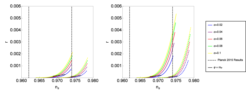
Figure 1: The predictions of power-law plateau inflation in a graph depicting the tensor to scalar ratio $r$ in terms of the spectral index $n_{s}$. Solid (dashed) lines correspond to $N=50$ ($N=60$) respectively. On the left we have $q=1$ and on the right $q=4$. $n$ increases along the length of the lines, counter-intuitively, right to left. The vertical black dashed straight lines represent the 1-$\sigma$ bounds on $n_{s}$ from the Planck data. The slanted solid black line depicts the limit below which values of $\varphi$ are sub-Planckian.

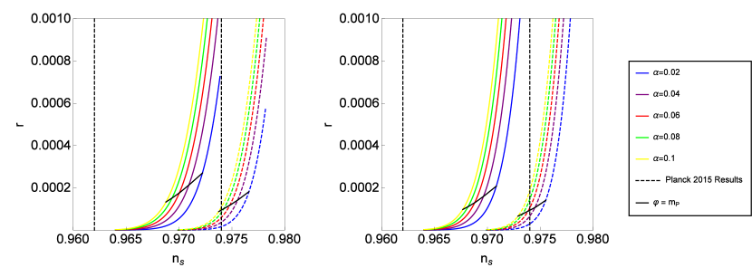
Figure 2: The predictions of power-law plateau inflation in a graph depicting the tensor to scalar ratio $r$ in terms of the spectral index $n_{s}$. Solid (dashed) lines correspond to $N=50$ $(N=60)$ respectively. On the left we have $q=1$ and on the right $q=4$. $n$ increases along the length of the lines, counter-intuitively, right to left. The vertical black dashed straight lines represent the 1-$\sigma$ bounds on $n_{s}$ from the Planck data. The slanted solid black line depicts the limit below which values of $\varphi$ are sub-Planckian.

We can see from Fig. 2 that sensible $n_{s}$ values exist in most cases but it would be better if $r$ were maximised to make contact with future observations. From the graph, it is clear that increasing $n$ decreases $r$. However, lowering $n$ increases $\varphi$ so we need to balance this whilst staying sub-Planckian. Increasing $q$ increases $r$ only marginally for all values of $n$ except $n=1$, but as shown in Fig. 3, $n=1$ is ruled out. However, again, this also increases $\varphi$. We can also see that a larger value of $\alpha$ is better for maximising our $r$ values, as expected since $r\propto\alpha^{\frac{2n}{n+2}}$ to lowest order in Eq. (8), this again also increases $\varphi$ though. Table 1 summarises these results.

	$n$ increased	$q$ increased	$\alpha$ increased
$n_{s}$	Substantially decreased	Marginally decreased	Complex pattern
$r$	Decreased (order of mag.)	Increased marginally (if $n\neq 1$)	Increases
$\varphi$	Decreased	Increased, impact reduced as $n$ grows	Increases

Table 1: Varying effects of the variables/parameters.

We can see from the graphs that irrespective of the $n$, $q$ and $\alpha$ choices a lower value of $N$ always produces a higher value of $r$, brings $n_{s}$ more acceptably within the Planck bounds and actually decreases $\varphi$ too. The value of $N$ is discussed in the next section. For now we will focus on the $N=50$ results, implying a low reheating temperature. Fig. 3 combines the variations of $\alpha$, $n$ and $q$ with the effects on $\varphi$ to show how the allowed parameter space for $n_{s}$ and $r$ varies. All values of $\alpha$ keep $n_{s}$ within the Planck bounds, the upper 1-$\sigma$ bound of which is shown by the black dashed lines in the panels of Fig. 3, while the lower bound is out of frame.

At this stage, considering only integer values of $n$ and $q$, it seems that $n=2$ is the best choice, as lower $n$ values give higher $r$ results (when allowed by $\alpha$) and $n=1$ is ruled out for all the sub-Planckian cases we are currently considering. Table 2 tabulates the values of $\alpha$ and $q$ which maximise $r$ for each $n$ and validates the expectation that $n=2$ provides the highest value. Higher values of $q$ do not provide the highest result because their $\alpha$ values are capped by the $\varphi<m_{P}$ criterion.

$n$	$q$	Max allowed $\alpha$	$n_{s}$	$r$
2	1	0.04	0.970463	0.000157
2	2	0.03	0.970474	0.000166
2	3	0.02	0.970472	0.000136
2	4	0.02	0.970478	0.000157
3	1	0.10	0.968504	0.000111
3	2	0.08	0.968518	0.000112
3	3	0.07	0.968523	0.000113
3	4	0.06	0.968524	0.000105
4	1	0.16	0.967203	0.000080
4	2	0.14	0.967218	0.000084
4	3	0.12	0.967223	0.000079
4	4	0.11	0.967225	0.000077

Table 2: Maximum values that $\alpha$ can take for specific combinations of $n$ and $q$ when $N=50$ whilst $\varphi$ remains sub-Planckian, and the corresponding values of $n_{s}$ and $r$.

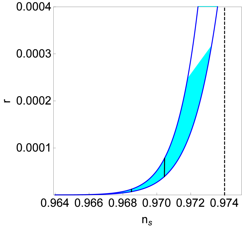
(a) $\alpha=0.01$

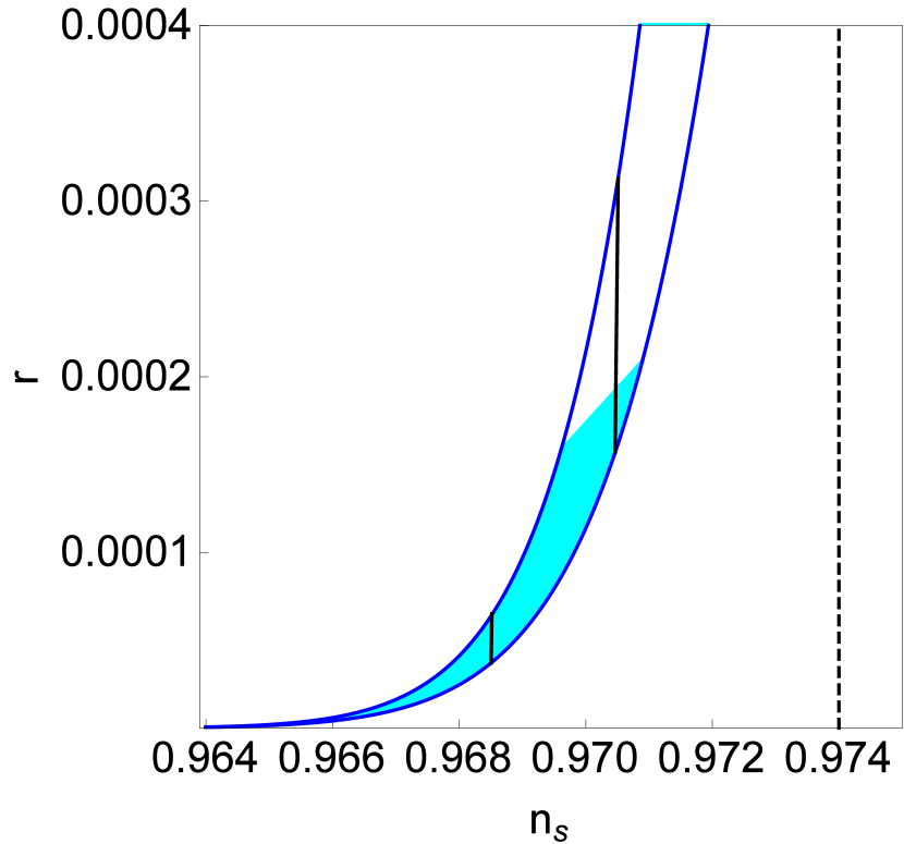
(b) $\alpha=0.04$

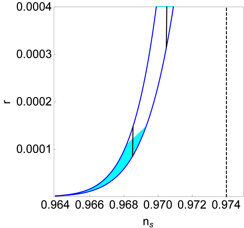
(c) $\alpha=0.08$

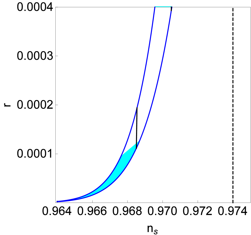
(d) $\alpha=0.1$

Figure 3: The predictions of power-law plateau inflation in a graph depicting the tensor to scalar ratio, $r$, in terms of the spectral index $n_{s}$, assuming $N=50$. The blue shaded region in each plot shows the range of values for $r$ and $n_{s}$ for the acceptable choices of $n$ and $q$ which maintain sub-Planckian $\varphi$. The lower blue line in each window shows $q=1$ and the higher $q=4$, however $n$ varies along the length of each line; $n=1$ is the highest point of each line and $n=10$ the lowest. The vertical solid black lines represent $n=2$ and $n=3$. Note that, counter-intuitively, $n=2$ is the line on the right-hand side and $n=3$ on the left. Note also that, in panel (d), the $n=2$ line is off the top of the graph and only the $n=3$ line is visible. The vertical black dashed line is the upper $n_{s}$ Planck 1-$\sigma$ bound.

3 Lowering $N$

So far we have examined the results for $n_{s}$ and $r$ when $N=50$ but perhaps it is possible to lower the value of $N$ further if we can manipulate when the epoch of reheating began. This section will investigate this and then examine how a period of thermal inflation may affect $N$.

3.1 Low Reheating Temperature

We start from the familiar equation:

$$N_{*}=62.8+\mathrm{ln}\Big{(}\frac{k}{a_{0}H_{0}}\Big{)}+\mathrm{ln}\Big{(}\frac{V_{\mathrm{end}}^{1/4}}{10^{16}\mathrm{GeV}}\Big{)}+\frac{1}{3}\mathrm{ln}\Big{(}\frac{g_{*}}{106.75}\Big{)}-\Delta N\,,$$ (10)

where $N_{*}$ is the number of remaining e-folds of inflation when the cosmological scales exit the horizon, $k=0.002\,$Mpc^-1 is the pivot scale, $V_{\mathrm{end}}$ is the energy density at the end of inflation, $g_{*}$ is the number of effective relativistic degrees of freedom at reheating and

$$\Delta N\simeq\frac{1}{3}\mathrm{ln}\Big{(}\frac{V_{*}^{1/4}}{T_{\mathrm{reh}}}\Big{)}\,,$$ (11)

where $V_{*}$ is the energy density when the cosmological scales exit the horizon and we assume that between the end of inflation and reheating the Universe is dominated by the inflaton condensate coherently oscillating in a quadratic potential around its vacuum expectation value. The latest data gives $V_{*}^{1/4}<2\times 10^{16}\,\mathrm{GeV}$ [1]. Assuming that $T_{\mathrm{reh}}$ is greater than the electroweak (EW) scale (to allow EW-baryogenesis), we have:

$$\Delta N\lesssim\frac{1}{3}\mathrm{ln}\Big{(}\frac{V^{1/4}_{\rm*\;max}}{T_{\mathrm{reh}}^{\mathrm{min}}}\Big{)}\simeq\frac{1}{3}\mathrm{ln}\Big{(}\frac{2\times 10^{16}\,\mathrm{GeV}}{200\,\mathrm{GeV}}\Big{)}\simeq 10.8\,,$$ (12)

which validates our choice to use the $N=50$ value, but does not introduce any lower values.

3.2 Thermal Inflation

Thermal inflation is a brief period of inflation possibly occurring after the reheating from primordial inflation. This second bout of inflation would allow the further reduction of the number of primordial e-folds of inflation. It occurs in the period between a false vacuum dominating over thermal energy density and the onset of a phase transition which cancels the false vacuum, when the thermal energy density falls to a critical value. The dynamics of thermal inflation are determined by a so-called flaton field, which is typically a supersymmetric flat direction lifted by a negative soft mass [10]. The scalar potential for the thermal flaton field is of the form:

$$V=V_{0}-\frac{1}{2}m^{2}\phi^{2}+\frac{1}{2}g^{2}T^{2}\phi^{2}+\cdots$$ (13)

where $m$ is the tachyonic mass of the field and $g$ is the coupling to the thermal bath, with the ellipsis denoting non-renormalisable terms that stabilise the zero-temperature potential. From the above, the effective mass-squared of the flaton field is

$$m_{\mathrm{eff}}^{2}=g^{2}T^{2}-m^{2}.$$ (14)

For high temperatures $m_{\rm eff}^{2}$ is positive and the flaton field is driven to zero, where $V=V_{0}>0$. This false vacuum density dominates when the thermal bath temperature drops to the value $T_{1}$ such that

$$\rho_{T}(T_{1})=\frac{\pi^{2}}{30}g_{*}T_{1}^{4}\equiv V_{0}\;\Rightarrow\;T_{1}=\Big{(}\frac{30}{\pi^{2}g_{*}}\Big{)}^{1/4}V_{0}^{1/4}\sim V_{0}^{1/4},$$ (15)

where $\rho_{T}$ is the density of the thermal bath. At $T_{1}$, thermal inflation begins and it continues until the temperature decreases enough that $m_{\rm eff}^{2}$ ceases to be positive. This critical temperature is

$$m_{\mathrm{eff}}^{2}(T_{2})\equiv 0\;\Rightarrow\;T_{2}=m/g\,,$$ (16)

when the effective mass-squared becomes tachyonic and a phase transition occurs, which sends the flaton field to the true vacuum, thereby terminating thermal inflation.

The total e-folds of thermal inflation are estimated as

$$N_{T}=\mathrm{ln}\Big{(}\frac{a_{\mathrm{end}}}{a_{\mathrm{beg}}}\Big{)}=\mathrm{ln}\Big{(}\frac{T_{1}}{T_{2}}\Big{)}=\frac{1}{4}\mathrm{ln}\Big{(}\frac{30}{\pi^{2}g_{*}}\Big{)}+\mathrm{ln}\frac{gV_{0}^{1/4}}{m}\,,$$ (17)

where $a_{\mathrm{beg}}$ ($a_{\mathrm{end}}$) is the scale factor of the Universe at the beginning (end) of thermal inflation.

We also know

$$g\leq 1,\qquad m^{2}\langle\phi\rangle^{2}\sim V_{0},\qquad\langle\phi\rangle\leq m_{P}$$ (18)

resulting in

$$V_{0}^{\mathrm{max}}\sim(m\,m_{P})^{2}$$ (19)

Therefore:

$$N_{T}\leq\underbrace{\frac{1}{4}\mathrm{ln}\Big{(}\frac{30}{\pi^{2}g_{*}}\Big{)}}_{\simeq 0}+\mathrm{ln}\Big{(}g\sqrt{\frac{m_{P}}{m}}\Big{)}\leq\frac{1}{2}\mathrm{ln}\Big{(}\frac{m_{P}}{m}\Big{)}\,.$$ (20)

The maximum value we can allocate to $N_{T}$ and hence reduce our e-folds of primordial inflation by (since $N_{*}\rightarrow N_{*}-N_{T}$), would arise from minimising $m$. The minimum $m$ is given by the electroweak scale $m_{{}_{\rm EW}}\sim 1\,\mathrm{TeV}$ since $\phi$ particles are not observed in the LHC. Using these values we obtain:

$$N_{T}\leq\frac{1}{2}\mathrm{ln}\frac{m_{P}}{m_{{}_{\mathrm{EW}}}}\simeq 17$$ (21)

So, considering that 17 e-folds of thermal inflation occurred, we may lower the value of $N_{*}$ down to $33$ or so. However, this will affect the combinations of $n$, $q$ and $\alpha$ that are still able to maintain sub-Planckian $\varphi$. From the previous graphs we know that $n=2$ gives us higher values for $r$ than any higher integer $n$ value (since $n=1$ violates the $\varphi<m_{P}$ bound). For $n=2$, we find $39\leqslant N_{*}\leqslant 56$ are within the range of values in the Planck 2015 data for $n_{s}$. We also find that increasing $q$ has minimal effect on $r$. Hence, for simplicity, we set $q=1$. Because of this we highlight $n=2$ and $q=1$ (with $\alpha=0.05$) as our best result, corresponding to the potential:

$$V=V_{0}\,\frac{\varphi^{2}}{\varphi^{2}+m^{2}}\,.$$ (22)

The $n_{s}$ and $r$ results for this combination of variables are shown in Table 3. In this table, we also include results for the running of the spectral index which the Planck observations found as $\frac{\mathrm{d}n_{s}}{\mathrm{dln}k}=-0.003\pm 0.007$ [1]. In our model,

$$\frac{{\rm d}n_{s}}{{\rm d}\ln k}=-2\frac{n+1}{n+2}\left(N+\frac{n+1}{n+2}\right)^{-2}\left\{1+\frac{n^{2}-2nq-n}{n+2}\left[\frac{n(n+2)q}{\alpha^{2}}\left(N+\frac{n+1}{n+2}\right)\right]^{-\frac{n}{n+2}}\right\}$$ (23)

As shown in Table 3, our model is in excellent agreement with the Planck observations.

$n$	$q$	$\alpha$	$N$	$n_{s}$	$r$	$\frac{\mathrm{d}n_{s}}{\mathrm{d}N}$
2	1	0.05	39	0.962299	0.000283	-0.00095
2	1	0.05	49	0.969874	0.000202	-0.00061

Table 3: Results for $n_{s}$, $r$ and the running of the spectral index for the case $n=2$, $q=1$, $\alpha=0.05$ showing the extremal allowed values of $N$ for completeness ($39\leqslant N_{*}\leqslant 49$).

4 Single Mass Scale

In an attempt to make the model more economic, we consider that our model is characterised by a single mass scale $M$, such that $V_{0}^{1/4}=m\equiv M$. Under this assumption, the model is more constrained and more predictive. The scalar potential is

$$V=M^{4}\Big{(}\frac{\varphi^{n}}{\varphi^{n}+M^{n}}\Big{)}^{q}\,.$$ (24)

The inflationary scale is determined by the COBE constraint:

$$\sqrt{\mathscr{P}_{\zeta}}=\frac{1}{2\sqrt{3}\pi}\frac{V^{\frac{3}{2}}}{m_{P}^{3}V^{\prime}}\,,$$ (25)

where $\mathscr{P}_{\zeta}=(2.208\pm 0.075)\times 10^{-9}$. is the spectrum of the scalar curvature perturbation. From Eqs. (1) and (7) we obtain

$$\Big{(}\frac{M}{m_{P}}\Big{)}=(2\sqrt{3}\pi nq\sqrt{\mathscr{P}_{\zeta}})^{\frac{n+2}{n+4}}\Big{[}n(n+2)q\Big{(}N+\frac{n+1}{n+2}\Big{)}\Big{]}^{-\frac{n+1}{n+4}}.$$ (26)

Inputting the calculated values of $\alpha=M/m_{P}$ for when $M=m=V_{0}^{1/4}$ into the equations for $n_{s}$, $r$ and $\frac{dn_{s}}{d\ln k}$, we find the results shown in Table 4.

$n$	$q$	$N$	$n_{s}$	$r$	$\frac{\mathrm{d}n_{s}}{\mathrm{d}\,\mathrm{ln}k}$	$M$ ($\times 10^{15}\,$GeV)
2	1	39	0.962267	3.2$\times 10^{-6}$	-0.00095	1.39$\pm$0.01
2	1	49	0.969851	2.1$\times 10^{-6}$	-0.00061	1.24$\pm$0.01

Table 4: Values of $n_{s}$, $r$, $\frac{dn_{s}}{d\ln k}$ and $M$ when $m=V_{0}^{1/4}\equiv M$.

Whilst $n_{s}$ is well within the Planck bounds, the values for $r$ have dropped considerably due to the reduction in $\alpha=M/m_{P}\ll 1$, which is expected as $r\propto\alpha^{\frac{2n}{n+2}}$. Note that we find $M\sim 10^{15}\,$GeV, which is close to the scale of grand unification as expected.

5 Large-field Power-law Plateau Inflation

In this section, we consider $\alpha$ no longer capped by ensuring $\varphi<m_{P}$ but we still satisfy the bound $(\varphi/m)^{n}>1$. Higher $\alpha$ values produce higher $r$ values but also higher $n_{s}$ values so we must be wary our $n_{s}$ results do not migrate outside of the Planck bounds. To mitigate this, a lower $N$ value is again better, so we consider values down to 33. Table 5 presents the best values of $n_{s}$ and $r$ for a combination of $N$ and $\alpha$ values. To demonstrate how our model improves the tensor to scalar ratio and spectral index without any fine tuning, Table 6 shows the results for $N=50$ and 60 and how they sit inside the Planck bounds. Fig. 4 shows the best results for five $\alpha$ values with their respective best $N$ values. Fig. 5 shows the range of our results for the same $\alpha$ values over all allowed $N$ values which maintain $n_{s}$ within the 1-$\sigma$ Planck bounds, fitting perfectly into the Planck parameter space. If we allow our $n_{s}$ results to extend into the 2-$\sigma$ Planck parameter space we can also incorporate $N=60$.

$\alpha$	$N$	$n_{s}$	$r$	$\frac{\varphi}{m}$	$\frac{\mathrm{d}n_{s}}{\mathrm{d}\,\mathrm{ln}k}$
0.6	39	0.962687	0.003500	5.36	-0.00093
0.8	39	0.962828	0.004717	4.62	-0.00093
1	38	0.962023	0.006169	4.08	-0.00097
2	38	0.962756	0.013058	2.80	-0.00094
3	37	0.962551	0.021450	2.20	-0.00096
4	36	0.962358	0.031315	1.83	-0.00098
6	34	0.962012	0.056328	1.37	-0.00102
8	33	0.962768	0.085796	1.08	-0.00100

Table 5: Values of $n_{s}$ and $r$, with super-Planckian values of $\varphi$ (ensuring $\varphi>m$), $n=2$ and $q=1$. $N$ values chosen to maximise $r$ whilst keeping $n_{s}$ within the 1-$\sigma$ Planck bound. Note, as well, that because Planck observations suggest $-0.010\leqslant\frac{\mathrm{d}n_{s}}{\mathrm{dln}k}\leqslant 0.004$ at 1-$\sigma$ [1], the running of the spectral index also matches observations.

$N$	$\alpha$	$n_{s}$	$r$	$\frac{\mathrm{d}n_{s}}{\mathrm{dln}k}$
50	1	0.970932	0.004106	-0.00057
50	2	0.971421	0.008600	-0.00055
50	3	0.971910	0.013482	-0.00054
50	4	0.972399	0.018753	-0.00052
50	5	0.972888	0.024412	-0.00051
60	1	0.975682	0.003122	-0.00040
60	2	0.976055	0.006515	-0.00039
60	3	0.976429	0.010180	-0.00038
60	4	0.976802	0.014115	-0.00037
60	5	0.977175	0.018321	-0.00036

Table 6: Values of $n_{s}$ and $r$, with super-Planckian values of $\varphi$ (ensuring $\varphi>m$) for $N=50$ and $N=60$.

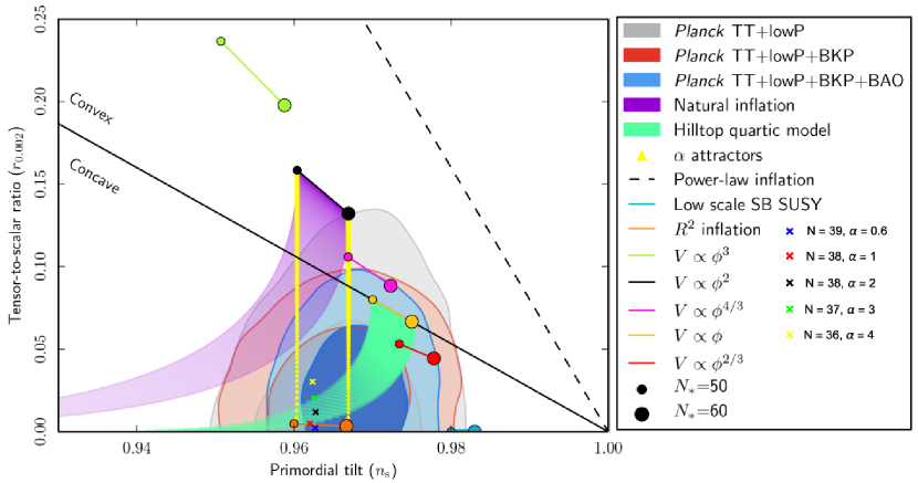
Figure 4: Super-Planckian power-law plateau inflation values of $n_{s}$ and $r$ superimposed on the Planck Graph.

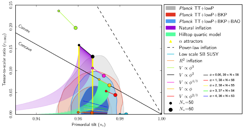
Figure 5: Super-Planckian power-law plateau inflation values of $n_{s}$ and $r$ superimposed on the Planck Graph, with $N$ varying between its min and max values for which $n_{s}$ is within the Planck 1-$\sigma$ bounds.

6 Supergravity Toy Model

In this section we will present a toy-model in supergravity (SUGRA) which can produce the scalar potential of Plateau Inflation for $n=2$ and $q=1$. We will follow the approach of Ref. [11] but only in form, not assuming the same theoretical framework (hence, we only consider a toy model) and with an important difference: we consider a minimal Kähler potential so that we can avoid producing too large $n_{s}$, but retain the successes of the $n=2$, $q=1$ Plateau Inflation model.

6.1 Global Supersymmetry

At first, we consider only global supersymmetry (SUSY) and sub-Planckian fields. We introduce the non-renormalisable superpotential:

$$W=\frac{S^{2}(\Phi_{1}^{2}-\Phi_{2}^{2})}{2m}\,,$$ (27)

where $S,\Phi_{1},\Phi_{2}$ are chiral superfields and $m$ is a large, but sub-Planckian scale. The F-term scalar potential is then

$$V_{F}=\frac{|S|^{2}}{m^{2}}\Big{[}|\Phi_{1}^{2}-\Phi_{2}^{2}|^{2}+|S|^{2}(|\Phi_{1}|^{2}+|\Phi_{2}|^{2})\Big{]}.$$ (28)

The above potential is minimised when $\Phi_{1}=\Phi_{2}$. Rotating the fields in configuration space (assuming a suitable R-symmetry) we can introduce a canonically normalised, real scalar field $\varphi$ such that $|\Phi_{1}|=|\Phi_{2}|\equiv\frac{1}{2}\varphi$. Then the scalar potential becomes

$$V_{F}=\frac{|S|^{4}\varphi^{2}}{2m^{2}}\,.$$ (29)

We consider that there is also a D-term contribution to the scalar potential. Mirroring Ref. [11], we take

$$V_{D}=\frac{1}{2}(|S|^{2}-\sqrt{2}M^{2})^{2},$$ (30)

where $M$ is the scale of a grand unified theory (GUT). Thus, in total, the scalar potential reads

$$V=\frac{|S|^{4}\varphi^{2}}{2m^{2}}+\frac{1}{2}(|S|^{2}-\sqrt{2}M^{2})^{2}.$$ (31)

Minimising the potential in the $S$ direction requires

$$\frac{\partial V}{\partial|S|}=0\;\Rightarrow\;\langle|S|^{2}\rangle=\frac{\sqrt{2}M^{2}}{1+\varphi^{2}/m^{2}}\,.$$ (32)

Inserting the above in Eq. (31) we obtain

$$V=\frac{M^{4}\varphi^{2}}{m^{2}+\varphi^{2}}\,,$$ (33)

which is the $n=2$, $q=1$ power-law plateau inflation model.

6.2 Local Supersymmetry

To confine ourselves in global SUSY we have to require that $M<m<\varphi<m_{P}$. Given that $\log(m_{P}/M)\simeq 2$, the available parameter space is not a lot. However, generalising the above into SUGRA may allow super-Planckian values for the inflaton, while $m\simeq m_{P}$. In SUGRA, we continue to consider the superpotential in Eq.(27) and we will also consider a minimal Kähler potential

$$K=|\Phi_{1}|^{2}+|\Phi_{2}|^{2}+|S|^{2}.$$ (34)

Then the F-term scalar potential is

$$V_{F} = \exp\left(\frac{|\Phi_{1}|^{2}+|\Phi_{2}|^{2}+|S|^{2}}{m_{P}^{2}}\right)\times$$ (35)

$$\left[\frac{|S|^{2}|\Phi_{1}^{2}-\Phi_{2}^{2}|^{2}}{m^{2}}\left(1+\frac{2|S|^{2}}{m_{P}^{2}}+\frac{|S|^{4}}{4m_{P}^{4}}\right)+\right.$$

$$\left.\frac{|S|^{4}(|\Phi_{1}|^{2}+|\Phi_{2}|^{2})}{m^{2}}\left(1+\frac{|\Phi_{1}^{2}-\Phi_{2}^{2}|^{2}}{4m_{P}^{4}}\right)-3\,\frac{|S|^{4}|\Phi_{1}^{2}-\Phi_{2}^{2}|^{2}}{4m^{2}m_{P}^{2}}\right].$$

Considering that $|S|$ is sub-Planckian, since $\langle|S|^{2}\rangle<\sqrt{2}M^{2}$, we have

$$V_{F}\simeq\exp\left(\frac{|\Phi_{1}|^{2}+|\Phi_{2}|^{2}}{m_{P}^{2}}\right)\left[\frac{|S|^{2}|\Phi_{1}^{2}-\Phi_{2}^{2}|^{2}}{m^{2}}+\frac{|S|^{4}(|\Phi_{1}|^{2}+|\Phi_{2}|^{2})}{m^{2}}\left(1+\frac{|\Phi_{1}^{2}-\Phi_{2}^{2}|^{2}}{4m_{P}^{4}}\right)\right].$$ (36)

Again, the potential is minimised when $\Phi_{1}=\Phi_{2}$. Writing $|\Phi_{1}|=|\Phi_{2}|\equiv\frac{1}{2}\varphi$, we obtain

$$V_{F}=e^{{}^{\frac{1}{2}(\varphi\!/\!m_{{}_{\!P}}\!)^{2}}}\frac{|S|^{4}\varphi^{2}}{2m^{2}}\,.$$ (37)

We consider the same D-term contribution to the scalar potential, given in Eq. (30). The total scalar potential is now

$$V=e^{{}^{\frac{1}{2}(\varphi\!/\!m_{{}_{\!P}}\!)^{2}}}\frac{|S|^{4}\varphi^{2}}{2m^{2}}+\frac{1}{2}(|S|^{2}-\sqrt{2}M^{2})^{2}.$$ (38)

Minimising the above along the $S$ direction, we find

$$\langle|S|^{2}\rangle=\frac{\sqrt{2}M^{2}}{1+e^{{}^{\frac{1}{2}(\varphi\!/\!m_{{}_{\!P}}\!)^{2}}}(\varphi/m)^{2}}\,.$$ (39)

Inserting this into Eq. (38) we obtain

$$V=\frac{M^{4}\varphi^{2}}{e^{{}^{-\frac{1}{2}(\varphi\!/\!m_{{}_{\!P}}\!)^{2}}}m^{2}+\varphi^{2}}\,.$$ (40)

Our finding is technically different from Eq. (33) because of the exponential factor in the first term in the denominator. However, this term is important only when $\varphi<m\simeq m_{P}$, when the exponential is unity. In the opposite case, when $\varphi>m\simeq m_{P}$, the first term in the denominator is negligible. So the exponential factor makes no difference and the potential is practically the same with the one in Eq. (33). This is certainly so if the inflaton remains sub-Planckian (i.e. when $m<m_{P}$).

Using the potential in Eq. (40) it can be checked that the $\eta$-problem of SUGRA inflation is overcome due to the D-term. In fact, one can show that $|\eta|\ll 1$ when $\varphi>m_{P}\simeq m$. However, for a super-Planckian inflaton, things are different from power-law plateau inflation, since the SUGRA correction dominates. So, our SUGRA toy model is similar but not identical to the the $n=2$, $q=1$ power-law plateau inflation model.

To have an idea of the value of the observables in this toy model, we can investigate the slow-roll parameters, which are found to be

$$\epsilon = \frac{2}{x}\frac{\alpha^{4}}{(\alpha^{2}+e^{\frac{1}{2}x}x)^{2}}\left(1+\frac{1}{2}x\right)^{2}\quad{\rm and}\quad$$ (41)

$$\eta = \frac{1}{x}\frac{2\alpha^{2}}{\alpha^{2}+e^{\frac{1}{2}x}x}\left[\frac{\alpha^{2}(1+2x)-3x}{\alpha^{2}+e^{\frac{1}{2}x}x}\left(1+\frac{1}{2}x\right)-\frac{1}{2}x^{2}\right],$$ (42)

where $x\equiv(\varphi/m_{P})^{2}$ and $\alpha$ is given in Eq. (4). Then the spectral index is

$$n_{s}-1=2\eta-6\epsilon=\frac{4}{x}\frac{\alpha^{4}}{(\alpha^{2}+e^{\frac{1}{2}x}x)^{2}}\left[\frac{\alpha^{2}(\frac{1}{2}x-2)-3x}{\alpha^{2}+e^{\frac{1}{2}x}x}\left(1+\frac{1}{2}x\right)-\frac{1}{2}x^{2}\right].$$ (43)

Taking $\varphi>m_{P}\Rightarrow x\gg 1$ and $\alpha\sim 1$ simplifies the above considerably as

$$\epsilon\simeq\frac{\alpha^{4}}{2xe^{x}}\quad{\rm and}\quad\eta\simeq-\alpha^{2}e^{-\frac{1}{2}x},$$ (44)

and it is evident that $|\eta|\ll 1$ as already mentioned. In this limit, it is easy to find

$$N=\frac{1}{4}\int_{x_{\rm end}}^{x}\frac{\alpha^{2}+e^{\frac{1}{2}x}x}{\alpha^{2}(1+\frac{1}{2}x)}\,dx\;\Rightarrow\;\alpha^{2}N\simeq\exp(x/2)\,,$$ (45)

where we have taken $x\gg x_{\rm end}$. Then, the observables become

$$n_{s}\simeq 1+2\eta\simeq 1-\frac{2}{N}\quad{\rm and}\quad r=16\epsilon\simeq\frac{4}{\ln(\alpha^{2}N)N^{2}}$$ (46)

These should be contrasted with the predictions of power-law plateau inflation given by Eqs. (8) and (9). At lowest order and taking $N\gg 1$ we find

$$n_{s}\simeq 1-\frac{3}{2N}\quad{\rm and}\quad r\simeq\frac{\sqrt{2}\alpha}{N^{3/2}}\,.$$ (47)

We see that the predictions of our SUGRA toy-model are more pronounced with respect to $N$, with both the spectral index and the tensor to scalar ratio smaller. Also, the dependence of $r$ on $\alpha$ is more prominent in the case of power-law plateau inflation. For more realistic values of the inflaton, however, where $\varphi\sim m_{P}\sim m$ (i.e. $x\sim 1$) we would expect $n_{s}$ and $r$ to lie inbetween the above extremes. Note that the predicted values are well in agreement with the Planck data, in all cases.

7 Conclusions

We have studied in detail a new family of inflationary models called power-law plateau inflation. The models feature an inflationary plateau, which is approached in a power-law manner, in contrast to the popular Starobinsky/Higgs inflation models (and their variants) but similarly to Shaft Inflation. We have shown that power-law plateau inflation is in excellent agreement with Planck observations.

To avoid supergravity corrections we mostly considered a sub-Planckian excursion for the inflaton in field space. As expected, this resulted in very small values for the ratio of the spectra of tensor to scalar curvature perturbation $r$. In an attempt to improve our results and produce observable $r$ we have considered minimising the remaining number of e-folds of primordial inflation when the cosmological scales exit the horizon. To this end, we assumed late reheating as well as a subsequent period of thermal inflation, driven by a suitable flaton field. We have managed to achieve $r\simeq 3\times 10^{-4}$ which might be observable in the future (see Table 3).

For economy we have also investigated the possibility that our model is characterised by a single mass scale. We have found that the spectral index of the scalar curvature perturbation $n_{s}$ satisfies well the Planck observations but the model produces unobservable $r$.

Abandoning sub-Planckian requirements allows the model to achieve much larger values of $r$. Indeed, for natural values of the mass scales (Planck and GUT scale), i.e. without fine-tuning, we easily obtain $r$ as large as a few percent (up to 9%, see Table 5), which is testable in the near future. Our predicted values for $r$ and $n_{s}$ fall comfortably within the 1-$\sigma$ bounds of the Planck observations, while different models of the power-law plateau inflation family are clearly distinguishable by future observations (see Figs. 4 and 5).

From our analysis, we have found that the best choice of model in the power-law plateau inflation family has the scalar potential $V=V_{0}\varphi^{2}/(m^{2}+\varphi^{2})$, which is also a member of the shaft inflation family of models [8].

Such a potential was originally introduced by S-dual inflation in Ref. [11], where, however, the inflaton was non-canonically normalised so the predicted value for $n_{s}$ was too large and incompatible with the Planck data. Following Ref. [11] but crucially considering canonically normalised fields (i.e. minimal Kähler potential) we have constructed a toy-model realisation in global and local supersymmetry for our preferred power-law plateau inflation model.

All in all, the level of success of power-law plateau inflation, and the fact that it offers distinct and testable predictions make this a worthy candidate for primordial inflation, which may well be accommodated in a suitable theoretical framework, as our toy models suggest.

Acknowledgements

CO is supported by the FST of Lancaster University. KD is supported (in part) by the Lancaster-Manchester-Sheffield Consortium for Fundamental Physics under STFC grant: ST/L000520/1.

References

- [1] P. A. R. Ade et al. [Planck Collaboration], arXiv:1502.02114 [astro-ph.CO]
- [2] K. Dimopoulos and C. Owen, arXiv:1606.06677 [hep-ph].
- [3] B. Garbrecht, C. Pallis and A. Pilaftsis, JHEP 0612 (2006) 038.
- [4] A. A. Starobinsky, Phys. Lett. B 91 (1980) 99; Sov. Astron. Lett. 9 (1983) 302.
- [5] F. L. Bezrukov and M. Shaposhnikov, Phys. Lett. B 659 (2008) 703.
- [6] R. Kallosh, A. Linde and D. Roest, JHEP 1311 (2013) 198; JHEP 1408 (2014) 052.
- [7] F. L Bezrukov, D.D Gorbunov, Phys. Lett. B 713 (2012) 365; A. Kehagias, A. M. Dizgah and A. Riotto, Phys. Rev. D 89 (2014) no.4, 043527.
- [8] K. Dimopoulos, Phys. Lett. B 735 (2014) 75; PoS PLANCK 2015 (2015) 037.
- [9] G. K. Chakravarty, G. Gupta, G. Lambiase and S. Mohanty, Phys. Lett. B 760 (2016) 263; G. K. Chakravarty, U. K. Dey, G. Lambiase and S. Mohanty, arXiv:1607.06904 [hep-ph]
- [10] D. Lyth, E. Stewart, Phys. Rev. D 53 (1995) 1784
- [11] A. de la Macorra and S. Lola, Phys. Lett. B 373 (1996) 299.