An algebraic multigrid method for $Q_{2}\,$–$\,Q_{1}\,$mixed discretizations of the Navier-Stokes equations

Abstract

Algebraic multigrid (AMG) preconditioners are considered for discretized systems of partial differential equations (PDEs) where unknowns associated with different physical quantities are not necessarily co-located at mesh points. Specifically, we investigate a $Q_{2}\,$–$\,Q_{1}\,$mixed finite element discretization of the incompressible Navier-Stokes equations where the number of velocity nodes is much greater than the number of pressure nodes. Consequently, some velocity degrees-of-freedom (dofs) are defined at spatial locations where there are no corresponding pressure dofs. Thus, AMG approaches leveraging this co-located structure are not applicable. This paper instead proposes an automatic AMG coarsening that mimics certain pressure/velocity dof relationships of the $Q_{2}\,$–$\,Q_{1}\,$discretization. The main idea is to first automatically define coarse pressures in a somewhat standard AMG fashion and then to carefully (but automatically) choose coarse velocity unknowns so that the spatial location relationship between pressure and velocity dofs resembles that on the finest grid. To define coefficients within the inter-grid transfers, an energy minimization AMG (EMIN-AMG) is utilized. EMIN-AMG is not tied to specific coarsening schemes and grid transfer sparsity patterns, and so it is applicable to the proposed coarsening. Numerical results highlighting solver performance are given on Stokes and incompressible Navier-Stokes problems.

1 Introduction

Multigrid methods are among the most efficient algorithms for solving sparse linear systems arising from discretized elliptic partial differential equations (PDE)s [1, 2]. Rapid convergence requires that the algorithm’s relaxation phase complement the coarse grid correction phase. Relaxation focuses on reducing oscillatory error components, often via a simple iteration. The coarse phase projects a residual equation to a coarse space and interpolates an associated coarse solution to correct the approximation. A hierarchy of resolutions result when the coarse solution is approximated by a recursive multigrid invocation. This paper is concerned with mixed finite element discretizations of PDE systems and an algebraic multigrid (AMG) method, which automatically constructs a mesh hierarchy and grid transfers. For PDE systems, constructing AMG components with the desired complementary properties is challenging, especially when there is strong coupling between different types of unknowns (e.g., pressures and velocities). Matrices that result from PDE systems are frequently far from the M-matrices that are generally more amenable to standard AMG methods. Among applications involving PDE systems, the saddle point nature of incompressible flow problems introduces additional complications. Standard multigrid relaxation algorithms do not typically smooth errors appropriately and algebraic multigrid procedures for generating grid transfers that partially rely on positive-definite matrix properties (such as smoothed aggregation) have difficulties as well. Further, traditional algebraic multigrid methods do not distinguish between unknown types. Thus, they might produce odd interpolation operators with stencils that mix unknown types, e.g., a fine pressure might interpolate from a set of coarse velocities.

Geometric multigrid methods have been developed for a range of PDE systems and discretizations (e.g., [2]). Much of this work has centered on effective relaxation techniques for specific PDE systems and so ideally one would like to leverage these techniques within an AMG approach. In geometric multigrid, inter-grid transfers are based on a geometrical relationship between meshes, such as using linear interpolation to transfer solutions across meshes. AMG methods are an attractive alternative for applications with complex meshes or features as formulating a mesh hierarchy and geometric inter-grid transfers is sometimes challenging.

One AMG approach (referred to as the point-based approach in [3]) for co-located PDE systems centers on coarsening spatial locations. By co-located, we refer to discretizations where degrees-of-freedom (dofs) associated with different physical quantities (e.g., pressures and electric fields) are situated at the same spatial location. For a co-located representation of the incompressible Navier-Stokes equations, each velocity dof is associated with a spatial location where there is a corresponding pressure dof. The discretization matrix can be viewed as a block operator with constant sized blocks, each corresponding to a unique spatial location. Standard AMG coarsening constructs a graph where each vertex is associated with one block matrix row and weighted edges between vertex $i$ and $j$ are defined based on some norm (or quantity) corresponding to the sub-matrix in the $i$th block row and the $j$th block column. Standard coarsening algorithms can then be employed accompanied by schemes (typically modest modifications of AMG methods for scalar PDEs) to define coefficients for the grid transfer operators such that coarse level dofs retain the co-located structure. Unfortunately, this PDE system AMG approach is not possible for mixed finite element discretizations in which fine level dofs are not co-located.

A second AMG approach (referred to as the unknown-based approach in [3]) also considers a block matrix representation, but now blocks are defined by different physical quantities (e.g., pressures) and different equation types (e.g., Navier-Stokes momentum equations, incompressibility condition, Maxwell-Faraday equations). Specifically, the matrix can be written as

$$\begin{bmatrix}A_{11}&A_{12}&\cdots&A_{1k}\\ A_{21}&A_{22}&\cdots&A_{2k}\\ \vdots&\vdots&\ddots&\vdots\\ A_{k1}&A_{k2}&\cdots&A_{kk}\\ \end{bmatrix}\begin{bmatrix}u_{1}\\ u_{2}\\ \vdots\\ u_{k}\\ \end{bmatrix}=\begin{bmatrix}f_{1}\\ f_{2}\\ \vdots\\ f_{k}\\ \end{bmatrix},$$ (1)

where each $u_{i}$ corresponds to a field (e.g., velocities in the $x,y,$ and $z$ directions).

An AMG algorithm can be developed by requiring that grid transfers have a block diagonal form:

$$P=\begin{pmatrix}P_{1}&&&&\\ &.&&&\\ &&.&&\\ &&&.&\\ &&&&P_{k}\end{pmatrix}.$$ (2)

Thus, coarse unknowns of one type do not directly influence interpolated unknowns of another type. The $P_{i}$ can be produced by $k$ separate invocations of an AMG method applied to matrices $\widetilde{A}_{ii}$. When $\widetilde{A}_{ii}=A_{ii}$, the AMG grid transfers ignore the PDE cross-coupling and so this might be problematic when the coupling is relatively strong. For mixed finite element representations that include an incompressibility condition, there is often a diagonal block of the PDE system that is identically zero, and so $\widetilde{A}_{ii}$ must be defined in another way (e.g., using Schur complement ideas).

This article follows a block interpolation approach. Our main innovation is to couple AMG invocations in a limited way. This is done to mimic certain features of a $Q_{2}\,$–$\,Q_{1}\,$discretization on coarse grids as $Q_{2}\,$–$\,Q_{1}\,$discretizations of the incompressible Navier-Stokes equations satisfy inf-sup conditions needed to produce stable discretizations [4, 5, 6]. It is generally desirable that all discretization operators within a multigrid method be stable as unstable coarse operators typically pose multigrid convergence problems (e.g., relaxation schemes may diverge). Obviously, geometric multigrid algorithms employing $Q_{2}\,$–$\,Q_{1}\,$discretizations on all levels satisfy inf-sup conditions throughout the hierarchy. We seek to emulate this within an AMG method by selecting coarse points in a fashion that loosely resembles coarse points within a geometric multigrid method. In particular, the selection of coarse velocities (used to define velocity interpolation) is obtained by first including velocities co-located with coarse pressures determined during a prior pressure AMG invocation. The set of coarse velocity unknowns is then augmented by velocity unknowns located at approximate mid-points between the coarse pressure unknowns. Numerical results will be given to demonstrate the effectiveness of this strategy when it is coupled to an energy minimization AMG algorithm [7], though the coarsening does not guarantee that resulting coarse discretizations satisfy inf-sup conditions. One key idea is that it is relatively easy to employ fairly general coarsening and grid transfer patterns within an energy minimization AMG (EMIN-AMG) framework. This is because this AMG variant (unlike most others) is fairly flexible with respect to different coarsenings and sparsity patterns. Other methods such as bootstrap AMG also have this property [8]. In addition to addressing stability concerns, it is expected that a careful choice of coarse variables will enhance the use of physics-based relaxation methods that rely heavily on sub-matrices accurately mirroring properties of associated PDE operators [6, 9].

The correlation of coarse unknowns between separate prolongator operators has been considered in different settings. In [10], multigrid transfers are motivated by recognizing that a standard geometric coarsening of the velocity mesh associated with a $\bm{P}_{1}$iso$\bm{P}_{2}\,$–$\,\bm{P}_{1}$ discretization corresponds to the pressure mesh. This leads to a shift strategy whereby the first coarsening of the velocity mesh is given by the pressure mesh (and the first velocity grid transfer could simply inject velocities located at nodes of the pressure mesh). Subsequent velocity grid transfers to the $\ell$th multigrid level use the AMG generated pressure grid transfer operator to the $\ell\hskip-2.8903pt-\hskip-2.8903pt1$th level. Coarse level stability is considered and alternative strategies retaining more fine level velocities are also proposed for $Q_{2}\,$–$\,Q_{1}\,$discretizations. While good convergence rates are obtained on several non-trivial problems, the approach uses a somewhat restrictive coarsening procedure that can result in multigrid cycles with an expensive cost. Our proposed algorithm seeks increased flexibility where one can use more aggressive coarsening rates to reduce the number of levels and the number of nonzeros per row (i.e., fill in) of the coarse operators, particularly important in a parallel setting.

Multigrid methods based on element agglomeration (AMGe) have also been considered for mixed finite element problems and mimetic discretizations [11, 12, 13]. In AMGe methods, additional topological information is maintained throughout all multigrid levels. While initially providing and maintaining this topological information has some challenges, its presence on coarse hierarchy levels can be leveraged in developing mixed fixed element AMG methods that satisfy key topological properties. Additionally, special multigrid methods for solid mechanics problems with contact and slide surfaces bear some resemblance to our proposed solver in that the coarsening of constraints associated with contact are correlated to the coarsening of displacement dofs [14]. As another example, AMG and fluid-structure interactions are described in [15, 16].

Before describing our AMG approach, we note that physics-based preconditioners are an alternative for PDE systems. These techniques also consider a block system such as (1) and can be viewed as approximate block factorizations involving Schur complement approximations. Here, AMG is used to approximate sub-matrix inverses needed within the approximate block factors. While physics-based preconditioners are effective and scalable, their convergence behavior is tied to the Schur complement approximations. The current paper is motivated by situations where monolithic multigrid can outperform several approximate block factorization preconditioners, though cases also exists where approximate block factorization preconditioners are better [17].

The paper is organized as follows. Section 2 briefly summarizes the considered PDEs and the $Q_{2}\,$–$\,Q_{1}\,$discretization. Section 3 illustrates a potential multigrid stability pitfall when velocity and pressure coarsenings are not correlated. Section 4 describes a new algorithm for constructing grid transfers while Section 5 completes the AMG description by detailing the multigrid relaxation. Numerical results are given in Section 6 followed by the conclusions in Section 7.

While our focus is on $Q_{2}\,$–$\,Q_{1}\,$discretizations, it is hoped that the techniques in this paper could be extended to other situations where one wishes to preserve specific properties of the fine level PDE discretization (e.g., mimetic representations) throughout a multigrid hierarchy.

2 Problem formulation

2.1 Discretization of the Stokes equations

The Stokes equations describe a model of viscous flow. Given a two- or three-dimensional domain $\Omega$, let $\bm{u}$ be a vector-valued function representing velocity, $p$ be a scalar function representing pressure, and $\bm{f}$ be a forcing term. The Stokes system is written as

$$\begin{array}[]{rcl}-\nabla^{2}\bm{u}+\nabla p&=&\bm{f}\quad\mbox{in}\;\Omega,\\ \nabla\cdot\bm{u}&=&0\quad\mbox{in}\;\Omega.\end{array}$$ (3)

It is complemented by a set of boundary conditions on $\partial\Omega=\partial\Omega_{D}\cup\partial\Omega_{N}$ given by

$$\bm{u}=\bm{w}\;\mbox{on}\;\partial\Omega_{D},\qquad\frac{\partial\bm{u}}{\partial\bm{n}}-\bm{n}p=\bm{s}\;\mbox{on}\;\partial\Omega_{N},$$ (4)

where $\bm{n}$ is the outward-pointing normal to the boundary and both $\bm{w}$ and $\bm{s}$ are given. If the velocity is specified on the whole boundary, i.e. $\partial\Omega_{D}=\partial\Omega$, then the compatibility condition

$$\int\limits_{\partial\Omega}\bm{w}\cdot\bm{n}=0$$ (5)

must be satisfied. In this case, pressure is unique only up to a constant.

A weak formulation of the Stokes equations is written as:

Find $\bm{u}\in\mathbf{H}^{1}(\Omega)$ and $p\in L_{2}(\Omega)$ such that

$$\begin{array}[]{rcll}\displaystyle\int\limits_{\Omega}\nabla\bm{u}:\nabla\bm{v}-\int\limits_{\Omega}p\nabla\cdot\bm{v}&=&\displaystyle\int\limits_{\partial\Omega_{N}}\bm{s}\cdot\bm{v}+\displaystyle\int\limits_{\Omega}\bm{f}\cdot\bm{v}&\mbox{for all}\;\bm{v}\in\mathbf{H}_{0}^{1}(\Omega),\\ \displaystyle\int\limits_{\Omega}q\nabla\cdot\bm{u}&=&0&\mbox{for all}\;q\in L_{2}(\Omega),\end{array}$$ (6)

where

$$\begin{array}[]{lcl}\mathbf{H}^{1}(\Omega)&=&\left\{\bm{u}\in\mathcal{H}^{1}(\Omega)^{d}\;|\;\bm{u}=\bm{w}\;\mbox{on}\;\partial\Omega_{D}\right\},\\ \mathbf{H}_{0}^{1}(\Omega)&=&\left\{\bm{v}\in\mathcal{H}^{1}(\Omega)^{d}\;|\;\bm{v}=\bm{0}\;\mbox{on}\;\partial\Omega_{D}\right\},\end{array}$$ (7)

with $d=2$ or $d=3$ being the spatial dimension.

The weak formulation (6) is discretized using finite-dimensional subspaces $\mathbf{X}^{h}\subset\mathbf{H}^{1}(\Omega)$, $\mathbf{X}_{0}^{h}\subset\mathbf{H}_{0}^{1}(\Omega)$ and $M^{h}\subset L_{2}(\Omega)$, and is written as:

Find $\mathbf{u}_{h}\in\mathbf{X}^{h}$ and $p_{h}\in M^{h}$ such that

$$\begin{array}[]{rcll}\displaystyle\int\limits_{\Omega}\nabla\mathbf{u}_{h}:\nabla\mathbf{v}_{h}-\displaystyle\int\limits_{\Omega}p_{h}\nabla\cdot\mathbf{v}_{h}&=&\displaystyle\int\limits_{\partial\Omega_{N}}\mathbf{s}\cdot\mathbf{v}_{h}+\displaystyle\int\limits_{\Omega}\bm{f}\cdot\mathbf{v}_{h}&\mbox{for all}\;\mathbf{v}_{h}\in\mathbf{X}_{0}^{h},\\ \displaystyle\int\limits_{\Omega}q_{h}\nabla\cdot\mathbf{u}_{h}&=&0&\mbox{for all}\;q_{h}\in M^{h}.\end{array}$$ (8)

Assuming that all $d$ components of velocity are approximated using the same scalar finite element space, this leads to a discrete Stokes problem

$$\begin{pmatrix}A_{S}&B^{T}\\ B&O\end{pmatrix}\begin{pmatrix}\mathbf{u}\\ \mathbf{p}\end{pmatrix}=\begin{pmatrix}\mathbf{f}_{\mathbf{u}}\\ \mathbf{f}_{\mathbf{p}}\end{pmatrix}.$$ (9)

Matrices $A_{S}$ and $B$ are block matrices, and have the following form for $d=2$:

$A_{S}=\begin{pmatrix}\widehat{A}_{S}&O\\ O&\widehat{A}_{S}\end{pmatrix}$, $B=\begin{pmatrix}B_{x}&B_{y}\end{pmatrix}$ and

$$\begin{array}[]{cclccl}\widehat{A}_{S}&=&[a_{ij}],&a_{ij}&=&\displaystyle\int\limits_{\Omega}\nabla\phi_{i}\cdot\nabla\phi_{j},\\ B_{x}&=&[b_{x,ki}],&b_{x,ki}&=&\displaystyle\int\limits_{\Omega}\psi_{k}\frac{\partial\phi_{i}}{\partial x},\\ B_{y}&=&[b_{y,ki}],&b_{y,kj}&=&\displaystyle\int\limits_{\Omega}\psi_{k}\frac{\partial\phi_{j}}{\partial y},\end{array}$$ (10)

where $\{(\phi_{1},0)^{T},\dots,(\phi_{m},0)^{T},(0,\phi_{1})^{T},\dots,(0,\phi_{m})^{T}\}$ is the basis of $\mathbf{X}_{0}^{h}$ and $\{\psi_{i}\}$ is the basis of $M^{h}$. The case $d=3$ is similar with the matrix $A_{S}$ being a $3\times 3$ block diagonal matrix with matrix $\widehat{A}_{S}$ on the diagonal, and the matrix $B$ having an additional directional component $B_{z}$ computed similarly to $B_{x}$ and $B_{y}$. For both $d=2$ and $d=3$ there is no coupling between velocity components for different directions.

Using a biquadratic approximation for velocity and a bilinear approximation for pressure in two dimensions produces a stable mixed method called the $Q_{2}\,$–$\,Q_{1}\,$, Taylor-Hood [18], approximation. The distribution of the dofs in the element is shown in Figure 1.

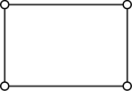
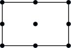
Figure 1: $Q_{2}\,$–$\,Q_{1}\,$pressure (left) and velocity (right) elements.

One important advantage of the $Q_{2}\,$–$\,Q_{1}\,$discretization is that it satisfies inf-sup or LBB stability conditions, and thus yields a stable discretization [4]. Approximations that do not satisfy this condition require the presence of an additional stabilization term, which introduces a stabilization matrix that replaces the zero block in (9).

2.2 Discretization of the Navier-Stokes equations

The steady-state Navier-Stokes equation system

$$\begin{array}[]{rcl}-\nu\nabla^{2}\bm{u}+\bm{u}\cdot\nabla\bm{u}+\nabla p&=&\bm{f}\quad\mbox{in}\;\Omega,\\ \nabla\cdot\bm{u}&=&0\quad\mbox{in}\;\Omega,\end{array}$$ (11)

with $\nu$ being a kinematic viscosity coefficient is complemented with boundary conditions given by

$$\bm{u}=\bm{w}\;\mbox{on}\;\partial\Omega_{D},\qquad\nu\frac{\partial\bm{u}}{\partial\bm{n}}-\bm{n}p=0\;\mbox{on}\;\partial\Omega_{N}.$$ (12)

Linearization and discretization of this system using a Picard iteration produces the Oseen system

$$\begin{pmatrix}A_{NS}&B^{T}\\ B&O\end{pmatrix}\begin{pmatrix}\mathbf{u}\\ \mathbf{p}\end{pmatrix}=\begin{pmatrix}\mathbf{f}_{\mathbf{u}}\\ \mathbf{f}_{\mathbf{p}}\end{pmatrix},$$ (13)

with $A_{NS}=\nu A_{S}+K$, where $K$ is a block diagonal matrix with matrix $\widehat{K}$ on the diagonal,

$$\widehat{K}=[k_{ij}],\qquad k_{ij}=\displaystyle\int\limits_{\Omega}(\mathbf{u}_{h}\cdot\nabla\phi_{j})\cdot\phi_{i}.$$ (14)

Here, $\mathbf{u}_{h}$ is the current estimate of the discrete velocity and once again a biquadratic basis is used for velocity while a bilinear basis is used for pressures to arrive at a $Q_{2}\,$–$\,Q_{1}\,$discretization of the Navier-Stokes equations. A quantitative measure of the relative contributions of the convection and diffusion terms is defined by the Reynolds number, which can be written as

$$\mathcal{R}=\frac{UL}{\nu},$$ (15)

where $U$ ($L$) is the characteristic velocity (length).

3 Coarse level stabilization

Discretization stability gives some measure of how well-posed the discrete problem is in comparison with the original continuous problem. It is well known in numerical analysis that the overall quality of a discretization can be expressed in terms of both consistency and stability. Stability concerns arise in the multigrid context due to the construction of the discretization operators associated with different resolutions within the hierarchy. Unfortunately, the stability of the finest level discretization does not guarantee that the coarse level operators of a multigrid hierarchy will also be stable. Instability of any coarse level operator typically leads to dramatic degradation in the overall multigrid convergence rates. This is often due to the fact that standard multigrid smoothers frequently diverge when applied to an unstable operator. Two well known areas where discretization stability concerns arise include PDEs with highly convective terms (even scalar PDEs) and saddle point systems. One possible remedy for highly convective systems lies in the use of Petrov-Galerkin style projections [19]. In this paper we mimic this idea by employing two separate EMIN-AMG invocations to generate interpolation and to generate restriction [7, 20]. To address saddle point stability concerns, which is the focus of this paper, we seek to encourage a relationship between the grid transfers for velocities and for pressures that mimics that of the $Q_{2}\,$–$\,Q_{1}\,$discretization.

The paper [10] discusses cases where instability of AMG coarse grid operators can appear and how this instability can lead to significant multigrid convergence degradation. Here, we give a rather elementary example to illustrate how easily instability can arise when the coarsening strategy for pressures and velocities is somewhat inconsistent. Specifically, consider the following simplified matrix which can be viewed as a marker-and-cell style approach [21] to a one dimensional PDE:

$$\begin{pmatrix}~{}I&B^{T}\\ -B&O\\ \end{pmatrix}\begin{pmatrix}u\\ p\end{pmatrix}=\begin{pmatrix}f\\ 0\end{pmatrix},$$ (16)

where

$$B^{T}=\begin{pmatrix}-1&1&\\ &.&.&\\ &&.&.&\\ &&&.&.&\\ &&&&-1&1\\ &&&&&-1&1\end{pmatrix}.$$ (17)

$B^{T}\in\mathbb{R}^{n\times n\hskip-0.72229pt-\hskip-0.72229pt1}$ can be viewed as a discrete gradient operator and $B$ as a divergence operator where pressure (velocity) unknowns are defined at circles (vertical lines) in the top image of Figure 2. Here, $n$ denotes the number of fine level pressure dofs.

Figure 2: One dimensional mesh. Top: fine pressure (velocity) unknowns denoted by circles (vertical lines). Bottom: coarse pressure (velocity) unknowns denoted by filled circles (boxes).

The Schur complement matrix, $BB^{T}$, is identical to that obtained by a standard three point central difference discretization of the Poisson operator with Neumann boundary conditions. Now consider a coarse mesh (bottom image of Figure 2) in conjunction with linear interpolation operators: $P_{v}$ and $P_{p}$. Thus, $P_{p}$ is a fairly standard geometric interpolation operator, and $P_{v}$ is close to standard geometric interpolation with the one exception that the choice of coarse points is somewhat sub-optimal. In this case, the stencil of the projected gradient, $P_{v}^{T}B^{T}P_{p}$, resembles a centered difference scheme, and the resulting projected operator is

$$\begin{pmatrix}~{}P_{v}^{T}P_{v}&P_{v}^{T}B^{T}P_{p}\\ -P_{p}^{T}BP_{v}&O\\ \end{pmatrix}.$$ (18)

The interior stencil of the Schur complement of the projected operator, $S=P_{p}^{T}BP_{v}(P_{v}^{T}P_{v})^{-1}P_{v}^{T}B^{T}P_{p}$, only weakly couples even and odd coarse grid points. In fact, the related operator $\widehat{S}=P_{p}^{T}BP_{v}P_{v}^{T}B^{T}P_{p}$ has completely decoupled even and odd points, i.e. $\widehat{S}_{i,i\pm 2}=-1,\widehat{S}_{i,i\pm 1}=0,\widehat{S}_{i,i}=2$. Both $S$ and $\widehat{S}$ are unstable Laplacians as indicated by the highly oscillatory eigenvector associated with the second smallest eigenvalue of $S$ shown in Figure 3.

Figure 3: Eigenvector associated with second smallest eigenvalue of Schur complement of projected system with coarse points as in Figure 2.

An oscillatory mode associated with a small eigenvalue of $S$ (or equivalently a large eigenvalue of $S^{-1}$) is an indication that we can generally expect $S^{-1}v$ to significantly amplify oscillatory components of a vector $v$. This instability is purely a function of the poor choice for the velocity coarse grid points. In fact, no instability is present in the resulting Schur complement if instead the coarse velocities are associated with mid-points between the pressures and linear interpolation is used.

$S$’s instability is likely to be problematic if AMG is applied to $S$ to further coarsen pressures and when a relaxation scheme is applied to (18). Further, we note that many specialized relaxation schemes developed for PDE systems rely on sub-matrix properties mirroring those of the corresponding PDE operators (e.g., $P_{v}^{T}B^{T}P_{p}$ mirroring a gradient operator). When this no longer holds, the specialized relaxation schemes may not smooth errors as expected.

4 AMG Grid Transfers for $Q_{2}\,$–$\,Q_{1}\,$discretizations

This section proposes an algorithm for generating grid transfers while the next section describes appropriate relaxation procedures. Together, these two components fully define an AMG method when used in conjunction with a Petrov-Galerkin projection process. The specific technique leverages the fact that a subset of the velocity unknowns are co-located with the pressure unknowns for $Q_{2}\,$–$\,Q_{1}\,$discretizations, which would not be the case for all types of mixed finite element discretizations. Let $A$ be a given full system matrix, $A=A_{NS}$ for concreteness. Algorithm 1 summarizes the setup of an AMG hierarchy given procedures for generating grid transfers and relaxation operators.

Algorithm 1 setup_hierarchy$(A_{\ell},x_{\ell},\ell,\ell_{max})$

$S_{\ell}=\mbox{{form\_relaxation}}(A_{\ell})$

if $\;\ell<\ell_{max}\;$ then

     $P_{\ell}=\mbox{{form\_interpolation}}(A_{\ell},x_{\ell})$

     $R_{\ell}=\mbox{{form\_restriction}}(A_{\ell},x_{\ell},P_{\ell})$

     $A_{\ell+1}=R_{\ell}A_{\ell}P_{\ell}$

     $x_{\ell+1}=\mbox{{project\_coordinates}}(x_{\ell},R_{\ell})$

     setup_hierarchy$(A_{\ell+1},x_{\ell+1},\ell+1,\ell_{max})$

end if

In Algorithm 1, $\ell_{max}$ is the number of levels in a multigrid hierarchy, $\ell=1$ corresponds to the finest level, the matrix $P_{\ell}$ defines interpolation from hierarchy level $\ell+1$ to level $\ell$ while $R_{\ell}$ defines restriction from $\ell$ to $\ell+1$. $A_{\ell}$ is the “discretization” matrix on the $\ell$th level (with $A_{0}=A$ being the finest level matrix), and $S_{\ell}$ is the smoother that is used within a relaxation procedure of the form

$$u_{\ell}^{k+1}=u_{\ell}^{k}+S_{\ell}(b_{\ell}-A_{\ell}u_{\ell}^{k}),$$

where $u_{\ell}^{k}$ is an approximation to the solution on level $\ell$, and $b_{\ell}$ is the right hand side on the same level. As our algorithms rely on coordinate locations $x_{\ell}$ (but not other mesh information), this is illustrated in the code fragment.

The discussion focuses on construction of interpolation matrices as the procedure for generating restriction operators only includes some modest differences. We also center the exposition on the principal themes while omitting some detailed graph heuristics. These details generally involve tie-breaking and weighing tradeoffs between including additional coarse points that might improve convergence, but increase iteration cost (and memory) due to increased coarse level fill-in. Many AMG codes have similar types of heuristics, and these are not the focus of this article. For the incompressible Navier-Stokes equations, our prolongators have the block diagonal form

$$P_{\ell}=\begin{pmatrix}P^{(v)}_{\ell}&O\\ O&P^{(p)}_{\ell}\end{pmatrix},$$

which is the same as (2) with slightly different notation to simplify the presentation. The basic idea is to apply an AMG algorithm to first generate a pressure prolongator $P^{(p)}_{\ell}$ followed by a procedure that generates a velocity prolongator $P^{(v)}_{\ell}$ using coarse points that are consistent with those used for $P^{(p)}_{\ell}$. By consistent, we mean that any coarse pressure point has co-located coarse velocity points as well as some notion of coarse velocity mid-points in between the co-located coarse points. The initial focus in our discussion is on coarse point selection and the choice of grid transfer sparsity patterns as these are the primary inputs to an energy minimization AMG algorithm. In addition to a consistent coarse point selection, we also aim to produce a multigrid algorithm with relatively sparse coarse grid operators. That is, we want coarsening rates and sparsity patterns to be defined in a way such that the matrix projection $R_{\ell}A_{\ell}P_{\ell}$ is not significantly denser than $A_{\ell}$. This requires some special considerations when biquadratic basis functions are employed on the finest level.

Algorithm 2 illustrates a general strategy. To simplify notation, level sub-scripts are omitted.

Algorithm 2 $P=\mbox{{form\_interpolation}}(A,x)$

$\left[\widetilde{A}^{(v)},\widetilde{A}^{(p)}\right]=\mbox{{form\_aux\_block\_diagonal}}(A)$

$C^{(p)}=\mbox{{find\_coarse\_pressure}}(\widetilde{A}^{(p)})$

$N^{(p)}=\mbox{{form\_pressure\_pattern}}(\widetilde{A}^{(p)},C^{(p)})$

$P^{(p)}=\mbox{{form\_pressure\_prolongator}}(\widetilde{A}^{(p)},C^{(p)},N^{(p)})$

$C^{(v)}=\mbox{{form\_coarse\_velocities}}(\widetilde{A}^{(p)},C^{(p)},N^{(p)},x)$

$N^{(v)}=\mbox{{form\_velocity\_pattern}}(\widetilde{A}^{(v)},C^{(v)})$

$P^{(v)}=\mbox{{form\_velocity\_prolongator}}(\widetilde{A}^{(v)},C^{(v)},N^{(v)})$

First, submatrices $\widetilde{A}^{(v)}$ and $\widetilde{A}^{(p)}$ are formed corresponding to velocity-velocity and presure-pressure coupling; subsequent AMG procedures will be applied to these matrices. While $A_{NS}$ could be used for $\widetilde{A}^{(v)}$, it may be advantageous to filter out weak couplings [22, 23]. Obviously, more care is required in defining $\widetilde{A}^{(p)}$ as the $(2,2)$ block of the PDE system matrix is identically zero. Coarse points are then defined. Specifically, $C^{(p)}$ and $C^{(v)}$ are sets of indices corresponding to the fine level degrees-of-freedom (pressures and velocities respectively) that will be represented on the next coarsest level. Formally, $C^{(p)}\subset\mathbb{Z}_{n^{(p)}}$ and $C^{(v)}\subset\mathbb{Z}_{n^{(v)}}$, where $n^{(p)}$ ($n^{(v)}$) is the number of fine grid pressures (velocities) and $\mathbb{Z}_{k}$ denotes the set of integers between $1$ and $k$ inclusive. Sparsity pattern matrices for the grid transfers are then constructed. For example, $N^{(p)}$ is a binary matrix indicating that $P^{(p)}_{ij}$ is nonzero only if $N^{(p)}_{ij}$ is one. Thus, the $j$th column of $N^{(p)}$ defines the support of the $j$th interpolating basis function. Finally, actual interpolation weights must be calculated. Given that coarse points and sparsity patterns will be chosen in somewhat nonstandard ways to preserve certain discretization features, it is important that a flexible algorithm is used to define interpolation weights. That is, the algorithm must not rely on restrictive assumptions concerning the distances between coarse points or the grid transfer sparsity patterns. For this, we employ an energy-minimizing framework (EMIN-AMG) [7], which is described further below.

4.1 Coarse points and sparsity patterns for pressure grid transfers

The $\widetilde{A}^{(p)}$ matrix must first be defined. A natural choice would be to take $\widetilde{A}^{(p)}=BB^{T}$ as this leads to a pressure Poisson operator, which often plays a central role within incompressible Navier-Stokes calculations. One complication, however, is that the stencil for this pressure Poisson operator is somewhat non-standard. In particular, the use of biquadratic basis functions for the velocities implies that stencils associated with $A_{NS},B$ and consequently $BB^{T}$ are wider/fuller than those obtained with standard first order finite differences, finite volumes, or finite elements. First order schemes typically give rise to fairly compact stencils involving only mesh points that immediately surround a central point. For example, the $Q_{2}\,$–$\,Q_{1}\,$interior stencils associated with $BB^{T}$ are 25 point stencils (as opposed to standard nine point stencils) when the mesh is a regular two-dimensional structured grid. To encourage stencil widths that more closely resemble standard first order discretizations, $\widetilde{A}^{(p)}$ is defined by dropping small entries in $Z=BB^{T}$ and lumping dropped entries to the diagonal so the sum of matrix entries within a row is preserved. This dropping essentially corresponds to removing nonzero entries that satisfy

$$|z_{ij}|\leq\tau_{1}\sqrt{|z_{ii}z_{jj}|},$$ (19)

with $\tau_{1}$ being a user provided parameter.

The other non-standard aspect of our AMG procedure for $P^{(p)}$ is that we orient the algorithm so that coarse pressure points are more distant than normal. In particular, classical AMG targets a set of coarse points that are distance two from each other in the associated matrix graph. Smoothed aggregation targets a set of aggregate root points (the aggregation counterpart to coarse points) that are distance three from each other. In our algorithm, we target distance four coarse points in the graph associated with $\widetilde{A}^{(p)}$. This choice is again driven by stencil widths within high order discretizations and avoiding excessive fill-in during the Petrov-Galerkin projection, $R_{\ell}A_{\ell}P_{\ell}$. When distance four coarse points are used in conjunction with the sparsity pattern to be discussed, the projection of $B$ (and $A_{NS}$) to coarser levels produce little additional fill-in (i.e. the average number of nonzeros per row does not rise appreciably). However, more traditional coarsening rate of three might be worth further exploration given the low complexity rates demonstrated in our numerical results with the coarsening rate of four.

Algorithm 3 $C^{(p)}=\mbox{{find\_coarse\_pressures}}(A,x)$

$[V,E]=\mbox{{form\_graph}}(A)$ $\triangleright$ $A\in\mathbb{R}^{n\times n}$, $V$ is the set of vertices, $E$ is the set of edges

$C^{(p)}=\varnothing~{};~{}F^{(p)}=\varnothing$ $\triangleright$ $C^{(p)}(F^{(p)})$ is a set of coarse (fine) vertices

$S=\{S_{i}\}_{i},\;S_{i}=\varnothing\hskip 14.45377pt\forall i\in\mathbb{Z}_{n}$

$Cand=\varnothing$

$k=\mbox{arbitrary vertex}$

while  $F^{(p)}\cup C^{(p)}\subsetneq\mathbb{Z}_{n}$  do

     $D_{3}=\{~{}j~{}|~{}dist(V_{k},V_{j},E)\leq 3~{}\}$  

     $D_{4}=\{~{}j~{}|~{}dist(V_{k},V_{j},E)=4~{}\}$

     $S_{j}=S_{j}\cup k\hskip 14.45377pt\forall j\in D_{3}$ $\triangleright$ $S_{j}$ updated to include all coarse points within distance 3 of $V_{j}$

     $D_{3}=D_{3}\setminus k$

     $C^{(p)}=C^{(p)}\cup k$

     $F^{(p)}=F^{(p)}\cup D_{3}$

     $Cand=Cand\cup D_{4}$

     $Cand=Cand\setminus(F^{(p)}\cup C^{(p)})$

     $[h_{1},h_{2}]=\mbox{{update\_heuristics}}(V,E,S,x,k,h_{1},h_{2})$

     $k=\operatorname*{arg\,min}_{j\in Cand}h_{1}(j)$ $\triangleright$ Best $Cand$ or arbitrary unmarked

     $\triangleright$ vertex if $Cand=\varnothing$                      

end while

$[C^{(p)},F^{(p)},S]=\mbox{{find\_extra\_dist3\_Cpoints}}(V,E,S,C^{(p)},F^{(p)},x,h_{1},h_{2})$

The general coarse point selection algorithm is given in Algorithm 3. The idea is to classify all $n^{(p)}$ vertices as either coarse points (represented on next coarse grid) or fine points (not represented on next coarse grid). In the AMG literature, these sets are respectively referred to as the $C$- and $F$-point sets, and the classification as a $C/F$-splitting. In this paper, we use $C^{(p)}$ and $F^{(p)}$ ($C^{(v)}$ and $F^{(v)}$) to refer to these two sets for pressure (velocity) vertices. Let $G=(V,E)$ be a graph of matrix $\widetilde{A}^{(p)}$. The classification is performed by first selecting an initial vertex, $k\in V$, and including it in $C^{(p)}$. All vertices within distance three from $k$, $dist(V_{k},V_{j},E)\leq 3$, (excluding $k$) are added to $F^{(p)}$. Here, distance refers to the minimum number of edge traversals (defined by $E$) required to travel from one vertex to another. A candidate set, $Cand$, is also introduced to encourage future coarse points to be distance four from existing $C^{(p)}$. Specifically, $Cand$ is the set of all vertices that are distance four from any $C^{(p)}$ and have not been already included in $C^{(p)}$ or $F^{(p)}$. The next $C$-point is selected giving priority to vertices in $Cand$ using heuristics that encourage the close packing of coarse points (by choosing a vertex with the smallest average Euclidean distance to existing $C^{(p)}$ points). The above procedure is repeated until all vertices are classified. Upon completion, all vertices in $C^{(p)}$ are at least distance four from each other. All vertices in $F^{(p)}$ are within distance three from at least one vertex in $C^{(p)}$. This may lead to situations where some $F^{(p)}$ vertices are not well covered by $C^{(p)}$ vertices, e.g. only within distance three from just a single $C^{(p)}$. This type of issue occurs in most algebraic multigrid codes (including our smoothed aggregation library) and can degrade convergence rates. To minimize these effects, heuristics are generally used to convert some $F^{(p)}$ vertices to $C^{(p)}$ vertices, targeting those not well covered by current $C^{(p)}$ vertices, i.e. those with a small size of set $S_{j}$ where for every $j\in F^{(p)}$ the set $S_{j}$ corresponds to all $C^{(p)}$ vertices that are within graph distance three from vertex $V_{j}$ ($j\in\mathbb{Z}_{n}$). Specifically, heuristics first convert $j\in F^{(p)}$ when $|S_{j}|=1$ and the Euclidean distance to the one $C^{(p)}$ point is large. Heuristics also examine points where $|S_{j}|=2$ and converts them to $C^{(p)}$ vertices only if the average Euclidean and the average graph distance to the $C^{(p)}$ vertices is large and if $j$ is far from the line segment connecting the two $C^{(p)}$ vertices. Typically, a small percentage of $C^{(p)}$ vertices are chosen by this algorithm. Harmonic averages (and standard averages) of Euclidean distances (and graph distances) to nearby $C^{(p)}$ vertices are stored in $h_{1}(j)$ (and $h_{2}(j)$). These are computed by update_heuristics. Harmonic averages essentially favor minimum distances.

To define $P^{(p)}$’s sparsity pattern the sets $S_{i}$ are used. The sparsity pattern is then given by

$$N^{(p)}_{ij}=\begin{cases}1,&\mbox{if $j\in S_{i}$},\\ 0,&\mbox{otherwise}.\end{cases}$$

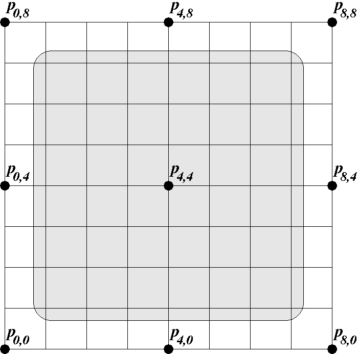
Figure 4: Left: $Q_{2}\,$–$\,Q_{1}\,$discretization where circles (boxes) are pressure and co-located velocity (non-co-located velocity) dofs. Right: perfect pressure coarsening. Circles are coarse pressure dofs. Dofs surrounded by gray rectangle belong to interpolation sparsity pattern associated with middle coarse dof’s column.

Figure 4 (right) illustrates a perfect coarsening of the pressure dofs for the discretization depicted in Figure 4 (left). Here, all nearest neighbors to any coarse pressure are exactly distance four away. This graph distance is in terms of the $\widetilde{A}^{(p)}$ matrix. Such a perfect coarsening would not generally occur, though our metrics encourage it. Consider, for example, the situation where the $p_{0,0}$ is the initial coarse vertex. Here, sub-script $i,j$ refers to the vertex that is $i$ ($j$) horizontal (vertical) edges away from the lowest-leftmost vertex. The $D_{4}$ and $Cand$ sets would include all vertices along the line between $p_{0,4}$ and $p_{4,4}$ inclusive and between $p_{4,4}$ and $p_{4,0}$ inclusive. To encourage perfect coarsening, the selection of a next $C$-point should favor vertices spatially closest to the initial corner vertex so that either $p_{0,4}$ or $p_{4,0}$ is chosen next. However, encouraging perfect coarsening becomes complicated as additional coarse vertices are chosen, and it is not necessary from a numerical convergence perspective. Finally, the gray shaded region illustrates the interpolation sparsity pattern associated with the $p_{4,4}$ vertex. In particular, all vertices surrounded by the gray region are at most distance three from $p_{4,4}$. Thus, these degrees-of-freedom would be nonzero in the column of the matrix interpolation operator associated with this $p_{4,4}$ coarse pressure.

4.2 Coarse points and sparsity patterns for velocity grid transfers

Each velocity component (in the different coordinate directions) is coarsened in an identical fashion and uses the same grid transfer sparsity pattern. The method for determining coarse velocity vertices is given in Algorithm 4. The algorithm starts by taking pressure coarse points, $C^{(p)}$, and adding pressure mid-points to define the set $\overline{C}^{(p)}$. The basic idea for mid-points is to first compute a set of target spatial locations $X_{i}$. The number of unique target locations is based on the number of unique $S_{i}$ sets. Recall, $S_{i}$ gives all coarse vertices used (i.e. with nonzero interpolation weights) when interpolating to the $i$th fine pressure vertex. Each target location corresponds to the geometric centroid (or barycenter) of the spatial locations associated with $S_{i}$’s coarse points. For each target location, we find the spatially closest fine pressure vertex. The search for the closest pressure is limited to the set of vertices $B_{i}$ which corresponds to all $F^{(p)}$ points within distance three to all of $S_{i}$’s vertices. Thus, the $B_{i}$ vertices define a small neighborhood surrounding the $i$th vertex. The closest pressure dof is chosen as a pressure mid-point only if it is not too close to an already to an already chosen coarse pressure in $\overline{C}^{(p)}$. Closeness is defined in a relative sense with respect to a box containing all $B_{i}$ and a tolerance, $tol$, shown in Algorithm 4. Further, the order in which our implementation computes target mid-points (the for loop in Algorithm 4) is such that vertices with larger $|S_{i}|$ are chosen before those with smaller $|S_{i}|$ ($|S_{i}|$ denotes the cardinality of the set $S_{i}$). In the final step, the coarse velocity points are taken to be velocities co-located with the chosen $\overline{C}^{(p)}$ pressures.

Algorithm 4 $C^{(v)}=\mbox{{find\_velocity\_Cpoints}}(S,C^{(p)})$

$\overline{C}^{(p)}=C^{(p)}$

for  $i\in F^{(p)}$  do

     $X_{i}=\left(\sum_{k\in S_{i}}x^{(p)}_{k}\right)/|S_{i}|$ $\triangleright$ Barycenter of surrounding $C$-points

     $B_{i}=\{j~{}|~{}j\in F^{(p)}\mbox{ and }S_{i}\subseteq S_{j}\}$ $\triangleright$ All $F$-points that also interpolate from $S_{i}$

     $t_{i}=\left(\sum_{k=1}^{d}\left(\max_{j\in B_{i}}x^{(p)}_{jk}-\min_{j\in B_{i}}x^{(p)}_{jk}\right)\right)^{1/2}$ $\triangleright$ Sum of box dimensions surrounding $B_{i}$

     $m=\operatorname*{arg\,min}_{k\in B_{i}}\|x^{(p)}_{k}-X_{i}\|_{*}$ $\triangleright$ Closest to target,$X_{i}$

     if  $\min_{j\in B_{i}\cap\overline{C}^{(p)}}\|x^{(p)}_{j}-x^{(p)}_{m}\|_{*}\geq\tau_{2}\;t_{i}$ then $\triangleright$ No nearby $\overline{C}^{(p)}$ vertex

         $\overline{C}^{(p)}=\overline{C}^{(p)}\cup\{m\}$

     end if

end for

$C^{(v)}=\mbox{{find\_colocated\_velocities}}(\overline{C}^{(p)})$

Algorithm 4’s cost is clearly proportional to the number of fine mesh vertices, $|F^{(p)}|$. Each fine vertex (i.e, each $i$ in the for loop) requires a constant amount of work, though this constant is not small. Specifically, this consists of the computation of $X_{i}$ and the set $B_{i}$ followed by calculations that are each proportional to the size of $|B_{i}|$. The $X_{i}$ computation is proportional to the number of $C^{(p)}$ vertices that are used to interpolate to the $i^{th}$ fine vertex (at most $2^{d}$ in the ideal uniform case). The sizes of the $B_{i}$ are bounded from above due to the PDE nature of the problem (meaning that for every fine point there is a bounded number of coarse points that are close) and the fact that coarse points interpolate to fine points only within distance three. The $B_{i}$ determination requires visiting a single coarse point from $S_{i}$ (any coarse point from the set is suitable) and checking if any of the fine points that interpolate from it also interpolate from all other points in $S_{i}$. On regular grids with perfect distance-four coarsening (e.g., Figure 4), the number of visited fine points is $7^{d}-1$ and $|B_{i}|$ is bounded by $3^{d-1}7^{d-1}$ (where again $d$ is the problem dimension).

The velocity prolongator sparsity pattern $N^{(v)}$ is defined exactly in the same fashion as for $N^{(p)}$ with the exception that each velocity component is treated separately. That is, a fine grid velocity associated with a coordinate direction only interpolates from coarse grid velocities associated with the same coordinate direction (i.e., $P_{\ell}^{(v)}$ is block diagonal with each block corresponding to a different coordinate direction). Specifically, nonzeros in the $i$th row of $N^{(v)}$ are given by all $C^{(v)}$ vertices that are within distance three of vertex $i$ within the nodal graph of $\widetilde{A}^{(v)}$. This $\widetilde{A}^{(v)}$ is defined by dropping small entries from $A_{NS}$ as previously discussed for $\widetilde{A}^{(p)}$.

Figure 5 illustrates an ideal case where

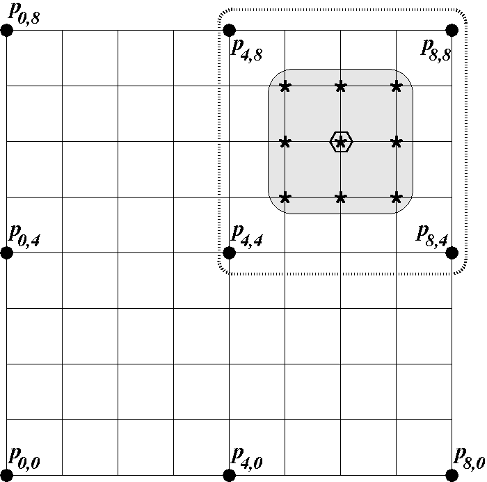
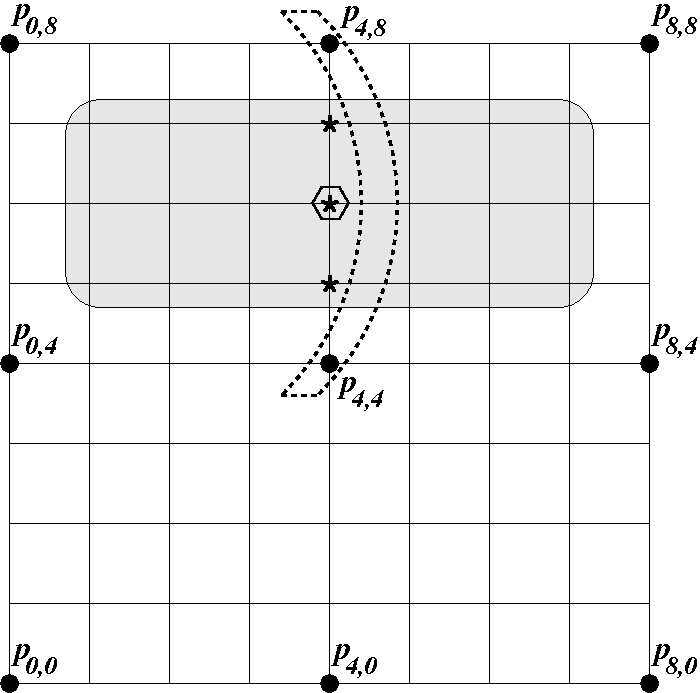
Figure 5: Two mid-point scenarios. Each ‘*’ vertex interpolates from the same subset of $C^{(p)}$, the solid dots within the dashed region. The hexagon gives the target spatial location and gray regions depict vertices that are searched to find a vertex near the target.

the original discretization is on a uniform regular mesh and all $C^{(p)}$ vertices are equi-spaced. Specifically, the right image depicts three vertices by a ‘*’. If we refer to these vertices as $k,\ell,$ and $m$, then $S_{k}\equiv S_{\ell}\equiv S_{m}$ consists of two vertices in the banana shaped region. The small hexagon gives the target spatial location ($X_{k}\equiv X_{\ell}\equiv X_{m}$) and vertices surrounded by the gray region define the $B_{k}\equiv B_{\ell}\equiv B_{m}$, all within distance three from both $S_{k}/S_{\ell}/S_{m}$ vertices. In this situation the target location is exactly at the same location as a pressure vertex. The left image shows the same information for a different mesh location. Figure 6 illustrates perturbed scenarios where the $p_{7,7}$ vertex is in $\overline{C}^{(p)}$ as opposed to the $p_{8,8}$ vertex. Thus, a heuristic has chosen a coarse point that is a distance three (instead of four) from existing coarse points. In this case, $p_{7,7}$ also lies within the $S$ sets associated with the ‘*’ vertices and the barycenters are offset. If $p_{6,6}$ is first added to $\overline{C}^{(p)}$ (due to the left image computation), then after $p_{5,6}$ might be added to $\overline{C}^{(p)}$ (the right image calculation) or deemed too close to $p_{6,6}$ depending on the value of a user provided $\tau_{2}$.

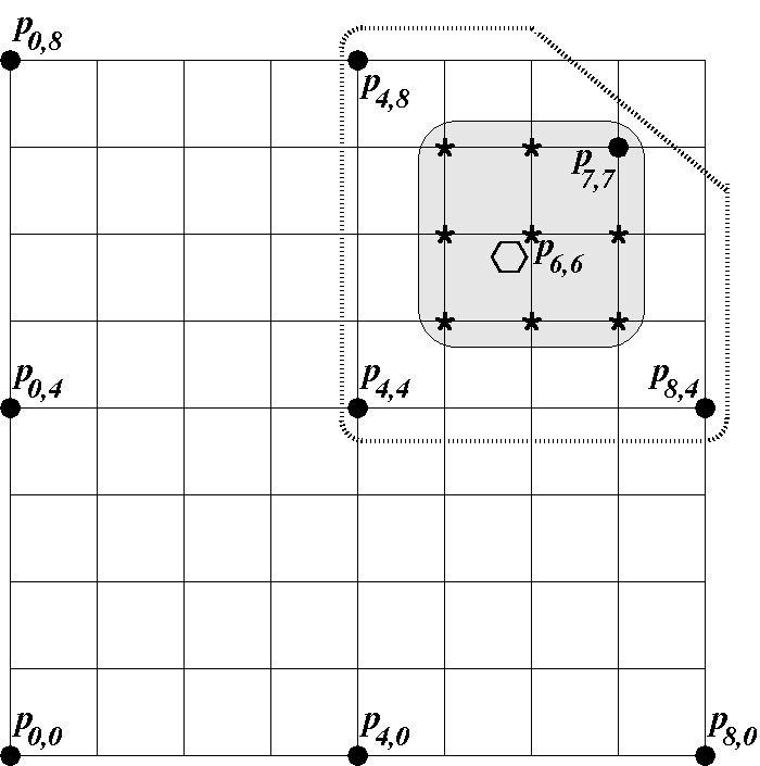
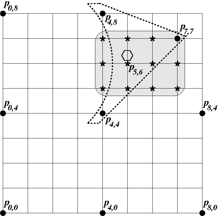
Figure 6: Perturbed mid-point scenarios. Each ‘*’ vertex interpolates from the same subset of $C^{(p)}$, the solid dots within the dashed region. The hexagon gives the target spatial location and gray regions depict vertices that are searched to find a vertex near the target.

That is, the total number of mid-points might vary somewhat with either several nearby mid-points or a sparser collection of mid-points. It is important to notice that even if the mid-point selection has some irregularities, this does not directly propagate to coarser levels. That is, coarse velocities at any given level are essentially a function of coarse pressures on that level and not a function of coarse velocities from a preceding level. Thus, a less than ideal mid-point selection does not have a direct influence on the coarsening of velocities on even coarser levels. Finally, additional heuristics are used to convert some $F^{(v)}$ vertices to $C^{(v)}$ vertices if some $F^{(v)}$ vertices are distant from all current $C^{(v)}$ vertices.

4.3 Determination of transfer coefficients using EMIN-AMG

There are several ways in which interpolation coefficients can be determined. Here, we use the energy-minimizing framework, EMIN-AMG, proposed in [7], which is a generalization of ideas in [24] and closely related to [25, 26, 27, 28, 29, 30, 31, 32]. We summarize only key features as the details are not crucial to this paper. Flexibility is the most significant aspect of EMIN-AMG for the present context. In particular, the EMIN-AMG algorithm does not make any implicit or explicit assumptions about the selection of coarse points or grid transfer sparsity patterns. This frees one to choose these components in a way to preserve important features. These features might be discretization features (as in this paper) or they might be application features, such as cracks or interfaces that one wishes to maintain throughout the multigrid hierarchy. This flexibility is in contrast to popular AMG methods such as classical AMG [22, 23] or smoothed aggregation AMG [33] where the choice of coarse points (or aggregates), interpolation sparsity pattern, and interpolation coefficients is somewhat intermingled. Another AMG algorithm with similar flexibility is given in [8].

The main idea of EMIN-AMG is as follows. Let ${\cal N}$ be a set of matrices with a specific (previously specified) nonzero pattern and dimensions, and $W$ be a set of fine level modes (e.g., vectors) requiring exact interpolation. Prolongator coefficients are determined through an approximate solution of a constrained minimization problem

$$P=\operatorname*{arg\,min}\limits_{P}\sum\limits_{j}\|P_{j}\|_{\chi}^{2}\\ ~{}~{}~{}~{}~{}~{}\mbox{subject to}~{}\\ P\in{\cal N},\quad\mbox{and}\quad W\in range(P).$$ (20)

Here, $\chi$ is some matrix norm, $P_{j}$ is the $j$th column of $P$, and the sum is over all columns in $P$. For symmetric problems (e.g., $A_{S}$ and approximations to the pressure Schur complement), it is natural to take $\chi$ to be the $A$-norm. Likewise, it is reasonable to take $\chi$ to be the $A^{T}A$-norm for non-symmetric systems. While the solution of an optimization problem may seem onerous compared to the task of solving a linear system, only a rough approximate solution to (20) is needed and an iterative process can be started with a simple but good initial prolongator satisfying the constraints.

In our case, $W$ is just a single vector of all ones when constructing $P^{(p)}$. This corresponds to the requirement that a constant can be perfectly recovered by interpolation. For $P^{(v)}$, $W$ consists of two (three) vectors in two (three) dimensions. Each vector contains only zeros and ones and corresponds to a constant for a velocity component in each of the different coordinate directions. It follows that the constraint $W\in range(P)$ can be satisfied if the sum of all nonzeros in each row of $P$ is one (assuming that the sparsity pattern does not mix different velocity direction components). That is, a coarse level constant interpolates to a fine level constant. Thus, a simple initial feasible guess for an optimization algorithm applied to (20) just takes the binary sparsity pattern matrix and divides each entry by the number of nonzeros in each row. The minimization problem is solved iteratively, for instance, using Algorithms 2 or 3 from [7]. These algorithms essentially correspond to applying a constrained version of CG or GMRES to solve for a prolongator matrix. The key is that the overall cost of the prolongator construction is only modestly higher than that of a more conventional AMG procedure as only a couple of EMIN-AMG iterations are sufficient.

In symmetric cases, $R$ is taken as $P^{T}$. However, for the Navier-Stokes problem a Petrov-Galerkin projection is employed, i.e. $R\neq P^{T}$. An energy minimization procedure is also used for determining the $R$ matrix. This procedure employs the transposed sparsity pattern for $P$ and uses the $AA^{T}$-norm for $\chi$. This choice of $R$ generally leads to projected discretization operators with satisfactory stability properties even in the presence of strong convection. This is discussed further in [7, 20]

5 Smoothers

Our choice of smoothers is somewhat restricted as typical AMG smoothers such as Jacobi and Gauss-Seidel are ineffective on saddle-point systems due to their negative eigenvalues. Relatively standard incomplete factorizations such as ILU(1) can be used for AMG smoothers. As the sparsity pattern of the incomplete factors is closely connected to the sparsity pattern of the original matrix (e.g. the ILU(0) factors have the same sparsity pattern as the initial discretization matrix), the zero block in the discretization matrix can cause issues. In this paper, our ILU(1) implementation treats the matrix diagonal (including those within the zero block) as being nonzero to encourage fill-in within the part of the incomplete factors associated with the zero block. In addition to ILU(1), we consider two families of smoothers that specifically take advantage of the block structure: Vanka and Braess-Sarazin relaxation.

5.1 Vanka relaxation

Vanka smoothing was originally proposed in [34] for finite-difference schemes. Further analysis of Vanka methods for finite-element discretizations of the Stokes equations has been done in [35]. The Vanka scheme corresponds to an overlapping block Gauss-Seidel method. The blocks are defined by partitioning all dofs into overlapping sets $T_{i}$, $i=1,\dots,n^{(p)}$. The number of sets is the same as the number of pressure dofs when $Q_{2}\,$–$\,Q_{1}\,$elements are employed. Each $T_{i}$ can be defined algebraically by taking all column indices corresponding to nonzero entries in the $i$th row of $B$ along with the $n^{(v)}+i$th index. That is, each $T_{i}$ consists of a single pressure dof and all velocity dofs that are either co-located or adjacent (in the matrix graph) to this single pressure dof. This choice of blocks is motivated by the saddle point nature of the problem so that each block submatrix is also a saddle point matrix. To apply one step of Vanka relaxation to a linear system, $A{\bf x}={\bf f}$ where the current approximation is given by ${\bf x^{k}}$, one computes an update of the form

$${\bf x^{k+1}}={\bf x^{k}}+\omega R_{i}^{T}(R_{i}AR_{i}^{T})^{-1}R_{i}\left({\bf f}-\mathcal{A}{\bf x^{k}}\right).$$ (21)

Here, $R_{i}$ is a binary projection operator restricting a global vector to a local one corresponding to dofs in $T_{i}$, and $\omega$ is the under-relaxation parameter. The overall relaxation procedure is done in a Gauss-Seidel manner cycling through all sets $T_{i}$.

5.2 Braess-Sarazin relaxation

Braess-Sarazin algorithms were originally considered as a relaxation scheme for Stokes problems [36, 37], and later applied to Navier-Stokes equations [38]. Compared to Vanka relaxation, where the smoothing procedure relies on solving multiple local saddle-point problems, Braess-Sarazin relaxation solves a global problem, though greatly simplified.

A single step of the relaxation procedure can be written as

$$\begin{pmatrix}\bf{u^{k+1}}\\ \bf{p}^{k+1}\end{pmatrix}=\begin{pmatrix}\bf{u^{k}}\\ \bf{p}^{k}\end{pmatrix}+\begin{pmatrix}\frac{1}{\omega}D&B^{T}\\ B&O\end{pmatrix}^{-1}\left(\begin{pmatrix}\bf{f}\\ \bf{g}\end{pmatrix}-\begin{pmatrix}\widehat{A}&B^{T}\\ B&O\end{pmatrix}\begin{pmatrix}\bf{u^{k}}\\ \bf{p}^{k}\end{pmatrix}\right),$$ (22)

where $\widehat{A}$ is the velocity block of $A$, $D$ is a suitable preconditioner for $\widehat{A}$, and $w$ is a relaxation parameter. As

$$\begin{pmatrix}\frac{1}{\omega}D&B^{T}\\ B&O\end{pmatrix}^{-1}=\begin{pmatrix}I&\frac{1}{\omega}D^{-1}B^{T}\\ O&I\end{pmatrix}^{-1}\begin{pmatrix}\omega D&O\\ B&-\frac{1}{\omega}BD^{-1}B^{T}\end{pmatrix}^{-1},$$ (23)

a solution of a Schur complement system, $S=BD^{-1}B^{T}$, is required. In our experiments, the Schur complement is explicitly formed and solved approximately by a relaxation procedure, e.g. via several Gauss-Seidel iterations. The Braess-Sarazin smoother requires a practical choice of the matrix $D$. The original paper considered $D=\operatorname*{diag}(\widehat{A})$. While that choice performed reasonably well in our experiments, we found that faster convergence is achieved with $D$ being a diagonal matrix with entries $d_{ii}=\sum_{j}|(\widehat{A})_{ij}|$. That is, $d_{ii}$ is the sum of the absolute values in the $i$th row of $\widehat{A}$.

6 Numerical results

In this section, Stokes and Navier-Stokes problems are considered. $\bm{Q}_{2}$ elements are used to discretize velocities and $\bm{Q}_{1}$ elements are used to discretize pressure. The discrete problems were generated using the IFISS software package [39] (version 3.3) written in MATLAB. The proposed algorithms were prototyped in MATLAB using the MueMat package [40], and later implemented in C++ in the MueLu multigrid package [41]. All numerical results were produced with MueLu (as of Trilinos version 12.6) with a single exception of the unstructured circle-driven cavity problem that was solved with MueMat.

In all of our calculations, five Gauss-Seidel iterations are performed to approximate the solution of the Schur complement system within the Braess-Sarazin smoother (BS), and the relaxation parameter is set to $0.666$. The Vanka smoother’s under-relaxation parameter is fixed at $0.5$, though it was observed in [34] that higher Reynolds numbers would benefit from lower parameter values. Unless stated otherwise, GMRES is used as an iterative method with the residual tolerance for the stopping criteria chosen to be $10^{-6}$. All results in this section use $\tau_{1}=0.06$ in (19) for dropping small entries while constructing $\widetilde{A}^{(v)}$ and $\widetilde{A}^{(p)}$, and $\tau_{2}=\sqrt{1.5\cdot 10^{-3}}$ in Algorithm 4 to decide whether a candidate coarse velocity mid-point is sufficiently far from already chosen velocity coarse points so that it should be added as an additional coarse point.

6.1 Stokes lid-driven cavity problem

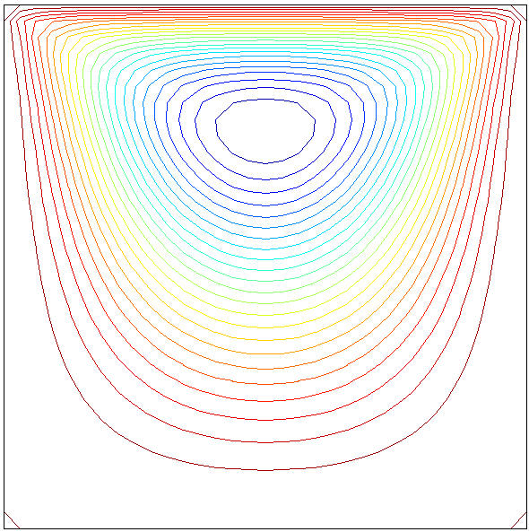
Figure 7: Equally distributed streamlines for the Stokes lid-cavity problem.

We begin with a benchmark lid-driven cavity Stokes problem on a square $\Omega=(-1,1)^{2}$ domain with leaky boundary conditions. Specifically, the $y$ component of velocity is zero on the boundary, i.e. $u^{(y)}|_{\partial\Omega}=0$. The $x$ component of velocity is only nonzero on the top of the cavity. In particular,

$$u^{(x)}=\begin{cases}1,&\mbox{for}\quad y=1;-1\leq x\leq 1,\\ 0,&\mbox{otherwise}.\end{cases}$$ (24)

We consider a set of uniform meshes. The discrete system has one zero eigenvalue corresponding to constant pressure. A typical solution on a $10\times 10$ mesh is illustrated in Figure 7. Prolongator coefficients are computed with a single EMIN-AMG CG step [7]. One iteration of the Vanka smoother or two iterations of Braess-Sarazin smoother are considered as pre- and post-smoothers in the multigrid hierarchy. Vanka relaxation is used on the coarsest grid instead of a direct solver to avoid direct solver issues associated with the singularity of the coarsest grid problem.

Table 1: Number of iterations and multigrid run times for the Stokes lid-driven cavity.

Dofs	Complexity	$\ell_{max}$	Vanka (1,1)			BS (2,2)			ILU(1) (1,1)
			Its	Setup	Solve	Its	Setup	Solve	Its	Setup	Solve
659	1.08	2	11	0.02	0.06	9	0.01	0.02	6	0.02	0.01
2467	1.08	2	12	0.05	0.20	10	0.03	0.03	7	0.05	0.02
9539	1.08	3	14	0.21	1.02	14	0.09	0.10	9	0.19	0.06
37507	1.08	3	15	0.93	4.38	19	0.36	0.36	10	0.77	0.22
148739	1.11	4	19	5.11	22.31	27	2.17	2.19	13	4.08	1.16
592387	1.05	5	18	28.84	84.80	20	13.34	6.70	17	20.32	5.96

Table 1 summarizes the results, including number of iterations and run times using a multigrid preconditioned GMRES solver. Our aggressive approach to coarsening (choosing coarse pressure dofs that are distance four from each other) results in a modest number of multigrid levels, where the coarsest hierarchy level for all examples has less than 205 total dofs. Further, the multigrid operator complexities are very small. These operator complexities are defined as the sum of the number of nonzeros of all discretization matrices on all levels divided by the number of nonzeros for the finest level discretization matrix. As the table illustrates, the number of additional nonzeros associated with the coarse level matrices is quite small and one can expect that the storage and computational time associated with these coarse operators is also quite modest. That is, the cost per iteration does not grow appreciably when more levels are employed. It is also particularly important that coarse discretization stencil widths do not grow too large on large scale parallel machines as large stencil widths imply longer distance communication.

Overall, the number of iterations remains relatively stable with Vanka and Braess-Sarazin smoothing which suggests an $h$-independence property of our approach (i.e., the number of iterations remains bounded as the mesh is refined). The generally well-behaved nature of the convergence rates is an indication that the AMG hierarchy (generated by the proposed coarsening, sparsity patterns, and EMIN-AMG) is suitable for this Stokes problem. Though the iterations do grow slowly with ILU(1) relaxation, it does require the least time in the solve phase for the meshes considered in this study. It is well known that the ordering of unknowns can have a significant influence on the convergence behavior when ILU methods are employed [42, 43]. For these Stokes experiments we found that a natural ordering (i.e., lexicographical starting from the lower-left corner) worked fine. However, a reverse Cuthill-McKee (RCM) ordering is needed to obtain satisfactory convergence rates with ILU for all the remaining Navier-Stokes examples shown in this paper. Overall, the Vanka run times are noticeably slower than Braess-Sarazin run times even though the convergence rate is a bit better. This iteration/run time behavior between Vanka and Braess-Sarazin has also been observed in [44]. The Vanka smoother involves numerous dense matrix solves associated with each Vanka block, which are of larger size due to the second order approximation in velocities. Additionally, residual components associated with velocity are updated multiple times by the Vanka smoother due to a significant overlap among Vanka blocks. It should be pointed out that our smoothing code has not been fully optimized.

With our current implementation, the setup phase requires more time than the solve phase. In general, the initialization time associated with the Braess-Sarazin smoother is small relative to the total AMG setup time while the Vanka and ILU(1) setup times are large. Roughly, the Vanka smoother setup time (or ILU(1) setup time) can be estimated by taking the difference between the total AMG setup time using Vanka (or ILU) and the total AMG setup time using Braess-Sarazin. Even with the Braess-Sarazin smoothing, the setup time is noticeable. The overwhelming majority of this time is spent on graph distance calculations, used in the coarsening and sparsity pattern calculation, and not in the EMIN-AMG algorithm. We believe that the large time for distance calculations is due to a poor implementation as opposed to intrinsic to the algorithm. While we have not further optimized this graph phase of the algorithm, it is important to note that the graph calculation is easily amortized over a nonlinear sequence of linear systems. That is, the graph coarsening can be performed just once over a sequence associated with a nonlinear solve. For the finest mesh associated with Table 1, the graph setup phase required 9.74 seconds. As this cost only needs to be incurred once, the incremental setup cost for an additional linear system using Braess-Sarazin would only be 3.60 seconds, which is about half the time of the solve phase.

Let us now examine the effect of the parameters $\tau_{1}$ and $\tau_{2}$ on our results. The parameter $\tau_{1}$ was introduced in Section 4.1. It is used for stencil reduction in matrices associated with velocity and pressure blocks. From a convergence point of view, smaller values of $\tau_{1}$ correspond to denser block matrices used in prolongators construction and thus result in more aggressive coarsening. On the other hand, larger values of $\tau_{1}$ correspond to sparser matrices and poorer approximations to the original matrices. Table 2 demonstrates the convergence for the lidcavity problem on a fixed mesh with varying values of $\tau_{1}$ while $\tau_{2}$ is fixed. The number of iterations reaches minimum at $\tau_{1}=0.05$ and increases thereafter. The size of the first coarse matrix increases from 28088 rows for $\tau_{1}=0$ to 74428 for $\tau_{1}=0.25$. Therefore, the selected $\tau_{1}$ is indeed a suitable choice for the problem. We expect it to be reasonable for Navier-Stokes problems with low Reynolds numbers.

The parameter $\tau_{2}$ was described in Section 4.2. It is responsible for determining the distance at which close points are considered to coincide. We found that our results are insensitive to this parameter. For instance, we found that the number of iterations remained constant for varying $\tau_{2}$ from $0.0$ to $0.4$. The parameter produced only a minor difference in the size of some coarse level matrices (e.g., it slightly reduced the size of the level 2 matrix for the 592387 mesh from 2739 for $\tau_{1}=0.01$ to 2199 for $\tau_{2}=0.4$).

Table 2: Number of iterations for the Stokes matrix of size 592387 with Braess-Sarazin smoother for varying values of $\tau_{1}$.

$\tau_{1}$	Number of iterations
0.00	100+
0.05	20
0.10	21
0.15	32
0.20	36
0.25	100+

We investigate the stability of the coarse grid operators by using a technique suggested in [45] (section 3.4.3) where a relationship between the smallest non-zero singular value of an off-diagonal matrix (in our case the scaled divergence operator) and the inf-sup constant $\beta$ is established. Instead of a looking at a sequence of matrices based on mesh refinement, we consider a sequence matrices derived from coarse level operators. Specifically, let $M_{0}^{(p)}$ and $M_{0}^{(v)}$ be pressure and velocity mass matrices associated with the fine level discretization. We denote by $M_{\ell}^{(p)}$ and $M_{\ell}^{(v)}$ the projections of these matrices to coarse levels, i.e.

$$M_{\ell}^{(p)}=R_{\ell}^{(p)}M_{\ell-1}^{(p)}P_{\ell}^{(p)},\quad M_{\ell}^{(v)}=R_{\ell}^{(v)}M_{\ell-1}^{(v)}P_{\ell}^{(v)},\quad\ell=1,\dots,\ell_{max}.$$ (25)

Let us also denote by $B_{\ell}$ the (2,1) block of the coarse operator $A_{\ell}$, corresponding to pressure rows and column velocities. Clearly, $B_{0}=B$ from equation (9). We then compute the smallest non-zero singular values $\sigma_{min,\ell}$ of the matrices

$$\widetilde{B}_{\ell}=\operatorname{lump}(|M_{\ell}^{(p)}|)^{-\frac{1}{2}}B_{\ell}\operatorname{lump}(|M_{\ell}^{(v)}|)^{-\frac{1}{2}}.$$ (26)

Table 3: Smallest non-zero singular values of matrices $\widetilde{B}_{\ell}$ for the Stokes matrix of size 592387.

$\ell$	0	1	2	3
$\sigma_{min,\ell}$	1.54	1.56	1.56	1.07

The results are shown in Table 3. The smallest singular values are clearly separated from 0 which suggests a similar stability of the operators, though the coarsest operator’s minimum singular value is somewhat lower (due in part to the small size, $150$ pressure dofs, of this matrix). The singular values for finer level matrices are all very close to each other.

6.2 Stokes circle-driven cavity problem

To test the solution strategy on unstructured meshes, we consider a modified form of the Stokes lid-driven cavity problem which we will call a circle-driven cavity problem. Specifically, the problem domain now corresponds to a square with a hole removed from the center. Figure 8 illustrates one of the coarser meshes. This mesh was generated with the Cubit software package [46]. While the mesh resembles a structured mesh near the domain corners, it is unstructured near the circular boundary. For our experiments, both velocity components are set to zero (via Dirichlet boundary conditions) along the box boundary. Additionally, Dirichlet conditions are applied on the circle boundary such that the velocity along the circle has a magnitude of one and is oriented in the clockwise tangent direction. That is, the horizontal (vertical) velocity is $1$ at the topmost (leftmost) side of the circle and $-1$ at the bottom (rightmost) side of the circle. Figure 9 illustrates the computed solutions on the mesh associated with 7097 elements. The dark ring in the figure corresponds to the circle boundary for $z=0$ (and is drawn to help clarify the plot).

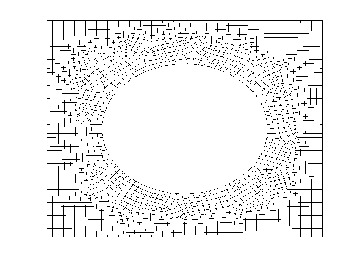
Figure 8: Unstructured mesh for the Stokes circle-driven cavity problem containing 1756 quadrilateral elements.

Figure 9: Computed horizontal (left) and vertical (right) velocity components for the Stokes circle-driven cavity problem. The rightmost portion of each figure corresponds to the top right corner of the cavity.

One can see that the horizontal and vertical prescribed values on the circular boundary gradually decay as they approach the outer cavity boundary.

Table 4 records the required number of GMRES iterations using the proposed multigrid preconditioner with both Vanka and Braess-Sarazin smoothing.

Table 4: Number of GMRES iterations for the Stokes circle-driven cavity problem.

Dofs	Complexity	$\ell_{max}$	Vanka (1,1)	BS (2,2)
1045	1.10	2	12	9
4078	1.12	3	13	12
16539	1.11	4	13	14
65343	1.10	4	14	18
261074	1.10	4	17	22
1043963	1.10	5	28	62

One can see that the iteration count grows quite modestly with respect to increases in mesh resolution (corresponding to a $1000$x increase in linear system size) similar to the structured grid tests with a slight uptick for the largest mesh. The exception is the Braess-Sarazin result on the largest mesh which we believe to be a result of a deficiency in Braess-Sarazin smoothing on steady problems. We have noticed the same sort of behavior in conjunction with geometric multigrid for meshes with irregular mesh spacing [44].

6.3 Navier-Stokes problems

Next, we consider the following problems for Navier-Stokes flow:

1. Lid-driven cavity problem

   The lid-driven mesh and boundary conditions are identical to the Stokes setup. Two values of $\nu$ are considered, $\nu=0.01$ and $\nu=0.002$ (corresponding to $\mathcal{R}=200$ and 1000, respectively).

2. Backward facing step problem

   An L-shaped domain is considered with a uniform mesh. A Poiseuille flow profile is imposed on the inflow boundary $(x=-1;0\leq y\leq 1)$, and a no-flow (zero velocity) condition is imposed on the walls. The outflow boundary $(x=L;-1<y<1)$ condition is set to Neumann, which automatically adjusts the mean outflow pressure to zero. Two values of $\nu$ are considered, $\nu=0.02$ and $\nu=0.005$ (corresponding to $\mathcal{R}=100$ and 400, respectively). The longer channel length $L=10$ is used for larger Reynolds numbers to allow for the exit flow to become well-developed (i.e., to have an essentially parabolic profile), while $L=5$ is used for smaller $\mathcal{R}$. Figure 10 demonstrates a typical solution for $\nu=0.02$.

3. Obstacle problem

   The obstacle problem has a similar setup to that of the backward facing step. In particular, $L=8$ (for both $\nu=0.02$ and $\nu=0.005$) and a uniform mesh is used to represent the domain. Additionally, a Poiseuille flow profile is imposed on the inflow boundary, no-flow condition is imposed on the walls and the same outflow boundary condition is imposed at the exit. Figure 11 demonstrates a typical solution for $\nu=0.02$.

As all of these problems are nonlinear, the matrix for AMG testing was chosen to be the last linear system within a converged Picard sequence that is terminated when a 2-norm of a nonlinear residual is less than $10^{-8}$. Prolongator coefficients and restriction coefficients are each computed with a single EMIN-AMG GMRES step. One iteration of the Vanka smoother as well as two iterations of Braess-Sarazin smoother are considered as a pre- and post-smoothers in the multigrid hierarchy.

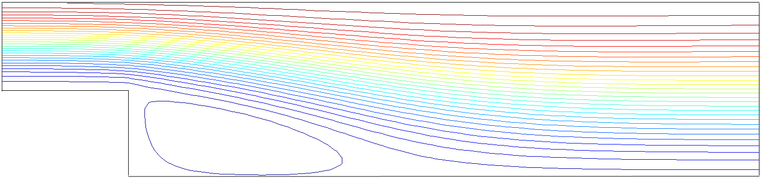
Figure 10: Equally distributed streamlines for the Navier-Stokes backward-facing step problem.

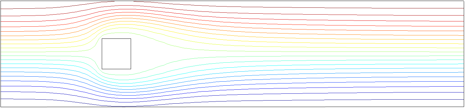
Figure 11: Equally distributed streamlines for the Navier-Stokes obstacle problem.

As the relative timing behavior is similar to the Stokes problem, we focus on convergence results for the Navier-Stokes problems. These are summarized in Table 6, Table 5, and Table 7 for each of the studied problems. Overall, the most important aspect of the convergence behavior is that the number of iterations is relatively stable with respect to mesh refinement, though there is certainly variation across the methods/problems and occasionally some modest growth. This generally gives us a certain level of confidence in the grid transfers and the overall stability of the coarse grid operators produced by the proposed combination of coarsening, grid transfer sparsity patterns and EMIN-AMG.

Similar to the Stokes problem, ILU smoothing generally leads to relatively consistent growth in iterations as the mesh is refined, though iterations dropped for the finest mesh lid-driven cavity problem when $\nu=0.005$. Some combinations of $\nu=0.005$ and coarse meshes are problematic with ILU smoothing. Though we have not performed a detailed study of these cases, we do note that for these mesh sizes there are stability concerns for the finest level Galerkin discretization when $\nu=0.005$. As with the Stokes problem, ILU smoothing often leads to the fewest iterations, though Vanka smoothing leads to the most scalable method with respect to iterations and mesh refinement. Interestingly, the number of iterations drops steadily when AMG is used with Vanka smoothing for the $\nu=0.005$ obstacle, though in other situations iterations are either nearly flat or rise modestly. While convergence rates are relatively constant with respect to mesh refinement, there is sensitivity to the Reynolds number. A noticeable Reynolds number dependence has been observed in other scalable solvers such as those discussed in [6]. Overall, the Braess-Sarazin smoother requires more iterations than the Vanka method as in the Stokes example. However, the gap between the two smoothers is somewhat larger than on the Stokes example, which perhaps suggests larger sensitivity of the Braess-Sarazin smoother to higher contributions of the convective terms. It should be noted that limitations of the Braess-Sarazin method have lead to more modern physics-based approaches such as the pressure convection-diffusion preconditioner and the least-squares commutator preconditioner that better account for the convective term [6]. We hope to explore this class of physics-based methods in the context of multigrid smoothers (as opposed to as preconditioners).

Table 5: Number of iterations for the Navier-Stokes lid cavity.

Dofs	$\nu=0.01$			$\nu=0.002$
	Vanka (1,1)	BS (2,2)	ILU(1) (1,1)	Vanka (1,1)	BS (2,2)	ILU(1) (1,1)
659	20	19	6	38	44	8
2467	26	22	7	49	55	9
9539	22	26	9	53	60	13
37507	24	36	18	59	68	31
148739	32	46	22	48	78	23

Table 6: Number of iterations for the Navier-Stokes backward-facing step.

$\nu=0.02$				$\nu=0.005$
Dofs	Vanka (1,1)	BS (2,2)	ILU(1) (1,1)	Dofs	Vanka (1,1)	BS (2,2)	ILU(1) (1,1)
479	20	21	6	889	51	56	5
1747	22	26	8	3287	49	58	6
6659	25	24	11	12619	43	58	18
25987	26	32	17	49427	37	53	24
102659	26	47	25	195619	47	68	46

Table 7: Number of iterations for the Navier-Stokes obstacle.

Dofs	$\nu=0.02$			$\nu=0.005$
	Vanka (1,1)	BS (2,2)	ILU(1) (1,1)	Vanka (1,1)	BS (2,2)	ILU(1) (1,1)
660	23	28	8	70	63	29
2488	23	33	8	41	62	17
9512	26	28	12	41	65	19
37168	24	32	14	34	51	22
146912	36	50	24	30	56	30

7 Conclusion

A new AMG coarsening approach has been proposed for $Q_{2}\,$–$\,Q_{1}\,$ mixed discretizations of Stokes and Navier-Stokes equations. The advantage of the new method is in its preservation of the spatial location relationship between pressure and velocity unknowns throughout multigrid hierarchy, so that the qualitative structure of the finest level is preserved on coarse levels. This is achieved by utilizing information gathered during pressure coarsening to guide the construction of the velocity grid transfer. The determination of grid transfer coefficients is then obtained by utilizing a flexible EMIN-AMG framework. A key feature of the proposed approach is that it coarsens fairly aggressively. In this way, the resulting multigrid operator complexity is quite low. This implies that the growth in the storage and in the V cycle cost remains quite modest as the number of multigrid levels increases. Experiments have been conducted with three different smoothers to demonstrate the suitability of the AMG hierarchy generated by the proposed procedures. Though there is some variation in iteration counts needed for convergence, the overall iteration/convergence rate trends are well-behaved. In several cases, the required number of iterations does not increase as the mesh is refined while in some other cases there is some modest iteration growth. Additionally, two of considered smoothers (Vanka and Braess-Sarazin) specifically target incompressible flow problems and rely somewhat on sub-matrices capturing basic attributes of corresponding PDE operators, which then must be maintained on coarse levels of the multigrid hierarchy.

The paper concentrated on the $Q_{2}\,$–$\,Q_{1}\,$ approximation due to it simplicity. However, it is hoped that the method can be extended to other mixed discretization methods based on the key idea that the coarsening of one type of variable guide the coarsening of other variables. One possible direction that we intend to explore are resistive magnetohydrodynamics (MHD) systems which also include electro-magnetic effects.

References

- [1] Briggs WL, Henson VE, McCormick SF. A multigrid tutorial: second edition. Society for Industrial and Applied Mathematics: Philadelphia, PA, USA, 2000.
- [2] Trottenberg U, Oosterlee CW, Schüller A. Multigrid. Academic press, 2001.
- [3] Fullenbach T, Stüben K. Algebraic multigrid for selected PDE systems. Proceedings of the 4th European Conference, Elliptic and Parabolic Problems, Bemelmans J, Brighi B, Brillard A, Chipot M, Conrad F, Shafrir I, V Valente GC (eds.), World Scientific, 2002; 399–409.
- [4] Brezzi F, Fortin M. Mixed and hybrid finite element methods. Springer-Verlag: New York, 1991.
- [5] Gunzburger M. Finite element methods for viscous incompressible flows. Academic Press: Boston, 1989.
- [6] Elman HC, Silvester DJ, Wathen AJ. Finite elements and fast iterative solvers: with applications in incompressible fluid dynamics. Oxford University Press, 2005.
- [7] Olson L, Schroder J, Tuminaro R. A general interpolation strategy for algebraic multigrid using energy minimization. SIAM Journal on Scientific Computing 2011; 33(2):966.
- [8] Brandt A, Brannick J, Kahl K, Livshits I. Bootstrap AMG. SIAM Journal on Scientific Computing 2011; 33(2):612–632.
- [9] Wesseling P. Principles of Computational Fluid Dynamics. Springer-Verlag: Berlin, 2001.
- [10] Wabro M. Coupled algebraic multigrid methods for the Oseen problem. Computing and Visualization in Science 2004; 7(3):141–151.
- [11] Lashuk I, Vassilevski P. Element agglomeration coarse Raviart-Thomas spaces with improved approximation properties. Numerical Linear Algebra with Applications 2012; 19(2):414–426.
- [12] Lashuk I, Vassilevski P. The construction of the coarse de Rham complexes with improved approximation properties. Computational Methods in Applied Mathematics 2014; 14(2):257–303.
- [13] Wabro M. AMGe—coarsening strategies and application to the Oseen equations. SIAM Journal on Scientific Computing 2006; 27(6):2077–2097.
- [14] Adams MF. Algebraic multigrid methods for constrained linear systems with applications to contact problems in solid mechanics. Numerical Linear Algebra with Applications 2004; 11(2-3):141–153.
- [15] Gee MW, K ttler U, Wall WA. Truly monolithic algebraic multigrid for fluid-structure interaction. International Journal for Numerical Methods in Engineering 2011; 85(8):987–1016.
- [16] Yang H, Zulehner W. Numerical simulation of fluid-structure interaction problems on hybrid meshes with algebraic multigrid methods. Journal of Computational and Applied Mathematics 2011; 235(18):5367 – 5379.
- [17] Cyr E, Shadid J, Tuminaro R, Pawlowski R, Chacon L. A new approximate block factorization preconditioner for 2D incompressible (reduced) resistive MHD. SIAM J. Sci. Comput. 2013; 35(3):B701–B730.
- [18] Taylor C, Hood P. A numerical solution of the Navier-Stokes equations using the finite element technique. Computers & Fluids 1973; 1(1):73–100.
- [19] Brooks AN, Hughes TJ. Streamline upwind/Petrov-Galerkin formulations for convection dominated flows with particular emphasis on the incompressible Navier-Stokes equations. Computer Methods in Applied Mechanics and Engineering 1982; 32(1):199–259.
- [20] Wiesner T, Tuminaro R, Wall W, Gee M. Multigrid transfers for nonsymmetric systems based on Schur complements and Galerkin projections. Numer. Lin. Alg. Appl. 2014; 21(3):415–438.
- [21] Harlow FH, Welch JE. Numerical calculation of time-dependent viscous incompressible flow of fluid with free surface. The Physics of Fluids 1965; 8:2182–2189.
- [22] Brandt A, McCormick S, Ruge J. Algebraic multigrid (AMG) for sparse matrix equations. Sparsity and Its Applications, Evans DJ (ed.). Cambridge University Press: Cambridge, 1984.
- [23] Ruge J, Stüben K. Algebraic multigrid (AMG), Frontiers in Applied Mathematics, vol. 3, chap. 4. SIAM: Philadelphia, PA, 1987; 73–130.
- [24] Mandel J, Brezina M, Vaněk P. Energy optimization of algebraic multigrid bases. Computing 1999; 62(3):205–228.
- [25] Brandt A. General highly accurate algebraic coarsening. Electronic Trans. Num. Anal 2000; 10:1–20.
- [26] Brandt A. Multiscale scientific computation: Review 2001. Multiscale and Multiresolution Methods, Springer Verlag, 2001; 1–96.
- [27] Brannick J, Zikatanov L. Algebraic multigrid methods based on compatible relaxation and energy minimization. Domain Decomposition Methods in Science and Engineering XVI, Lecture Notes in Computational Science and Engineering, vol. 55, Widlund O, Keyes DE (eds.). Springer: Berlin, 2007; 15–26.
- [28] Kolev TV, Vassilevski PS. AMG by element agglomeration and constrained energy minimization interpolation. Numer. Linear Algebra Appl. 2006; 13(9):771–788.
- [29] Vassilevski PS. General constrained energy minimization interpolation mappings for AMG. SIAM J. Sci. Comput. 2010; 32(1):1–13.
- [30] Wagner C. On the algebraic construction of multilevel transfer operators. Computing August 2000; 65:73–95.
- [31] Wan WL, Chan TF, Smith B. An energy-minimizing interpolation for robust multigrid methods. SIAM J. Sci. Comput. 2000; 21(4):1632–1649.
- [32] Xu J, Zikatanov L. On an energy minimizing basis for algebraic multigrid methods. Computing and Visualization in Science October 2004; 7:121–127(7).
- [33] Vaněk P, Mandel J, Brezina M. Algebraic multigrid by smoothed aggregation for second and fourth order elliptic problems. Computing 1996; 56(3):179–196.
- [34] Vanka SP. Block-implicit multigrid solution of Navier-Stokes equations in primitive variables. Journal of Computational Physics 1986; 65(1):138–158.
- [35] MacLachlan S, Oosterlee C. Local Fourier analysis for multigrid with overlapping smoothers applied to systems of PDEs. Numerical Linear Algebra with Applications 2011; 15(4):751–774.
- [36] Braess D, Sarazin R. An efficient smoother for the Stokes problem. Applied Numerical Mathematics 1997; 23(1):3–19.
- [37] Larin M, Reusken A. A comparative study of efficient iterative solvers for generalized Stokes equations. Numerical linear algebra with applications 2008; 15(1):13–34.
- [38] John V, Tobiska L. Numerical performance of smoothers in coupled multigrid methods for the parallel solution of the incompressible Navier-Stokes equations. International Journal for Numerical Methods in Fluids 2000; 33(4):453–473.
- [39] Elman HC, Ramage A, Silvester DJ. Algorithm 866: IFISS, a Matlab toolbox for modelling incompressible flow. ACM Trans. Math. Softw. Jun 2007; 33(2).
- [40] Gaidamour J, Hu JJ, Tuminaro RS, Siefert C. MueMat: a Matlab toolbox to experiment with new multigrid preconditioners 2011. URL http://www.osti.gov/scitech/servlets/purl/1140699.
- [41] Prokopenko A, Hu JJ, Wiesner TA, Siefert CM, Tuminaro RS. MueLu User’s Guide 1.0. Technical Report SAND2014-18874, Sandia National Labs 2014.
- [42] ur Rehman M, Vuik C, Segal G. A comparison of preconditioners for incompressible Navier–Stokes solvers. International Journal for Numerical methods in fluids 2008; 57(12):1731–1751.
- [43] Dahl O, Wille SØ. An ILU preconditioner with coupled node fill-in for iterative solution of the mixed finite element formulation of the 2D and 3D Navier-Stokes equations. International Journal for Numerical Methods in Fluids 1992; 15(5):525–544.
- [44] Adler JH, Benson TR, Cyr EC, MacLachlan SP, Tuminaro RS. Monolithic multigrid methods for two-dimensional resistive magnetohydrodynamics. SIAM Journal of Scientific Computing 2016; 38(1):B1–B24.
- [45] Boffi D, Brezzi F, Fortin M, et al.. Mixed finite element methods and applications. Springer, 2013.
- [46] Blacker T, Bohnhoff W, Edwards T. CUBIT mesh generation environment. Volume 1: Users manual. Technical Report SAND–94-1100, Sandia National Labs 1994.