Unconventional non-Fermi liquid state caused by nematic criticality in cuprates

Abstract

At the nematic quantum critical point that exists in the $d_{x^{2}-y^{2}}$-wave superconducting dome of cuprates, the massless nodal fermions interact strongly with the quantum critical fluctuation of nematic order. We study this problem by means of renormalization group approach and show that, the fermion damping rate $\left|\mathrm{Im}\Sigma^{R}(\omega)\right|$ vanishes more rapidly than the energy $\omega$ and the quasiparticle residue $Z_{f}\rightarrow 0$ in the limit $\omega\rightarrow 0$. The nodal fermions thus constitute an unconventional non-Fermi liquid that represents an even weaker violation of Fermi liquid theory than a marginal Fermi liquid. We also investigate the interplay of quantum nematic critical fluctuation and gauge-potential-like disorder, and find that the effective disorder strength flows to the strong coupling regime at low energies. Therefore, even an arbitrarily weak disorder can drive the system to become a disorder controlled diffusive state. Based on these theoretical results, we are able to understand a number of interesting experimental facts observed in curpate superconductors.

1 Introduction

A large amount of experimental and theoretical studies have been devoted to studying the unusual properties of high temperature cuprate superconductors in the past thirty years [1, 2, 3, 4, 5, 6, 7, 8, 9]. Although some consensuses have been reached, many fundamental problems are still in debate, including the microscopic pairing mechanism [1, 2, 7, 8, 9], the origin of pseudogap [2, 6], and the description of non-Fermi liquid behaviors of the normal state [1, 2, 3]. In the past decade, there have been accumulating experimental evidences for the existence of a strong anisotropy in many of the physical properties of YBa₂Cu₃O_6+δ (YBCO) [10, 11, 12] and Bi₂Sr₂CaCu₂O_8+δ (BSCCO) [13, 14]. Such an anisotropy is widely believed to be driven by the formation of a novel electronic nematic order [15, 16, 17, 18, 19], which spontaneously breaks the $C_{4}$ symmetry down to a $C_{2}$ symmetry. In case the nematic transition line goes across the superconducting transition line and penetrates into the superconducting dome, there exists a zero-temperature nematic quantum critical point (QCP). The nematic quantum phase transition and the associated quantum critical behaviors have been investigated extensively in recent years [20, 21, 22, 23, 24, 25, 26, 27, 28, 29, 30, 31].

From a theoretical perspective, there are two widely studied scenarios to induce an electronic nematic order. First, the nematic order can be generated by melting a stripe order that spontaneously breaks both translational and rotational symmetry [15, 16, 17, 18, 19]. The other way is related to Pomeranchuk instability which refers to the deformation of the shape of the Fermi surface of a metal due to Coulomb interaction [15, 16, 17, 18, 19, 32, 33, 34, 35]. In the simplest case, Pomeranchuk instability occurs when the circular Fermi surface of a two-dimensional metal becomes ellipse-like via quadrupolar distortion. [15, 16, 17, 18, 19]. The Hubbard model defined on square lattices [35, 39, 40, 41, 42, 43, 44] provides a pertinent platform to investigate the electronic nematic order. Halboth and Metzner [35] studied a two-dimensional Hubbard model using functional renormalization group (RG) method, and revealed Pomeranchuk instability and nematic order. More recently, the square lattice Hubbard model is studied by variational cluster approximation [45, 46] and found to display a local nematic phase under certain circumstances, which might be applied to understand the intra-unit-cell electronic nematicity observed in the scanning tunneling spectroscopy (STS) measurements by Lawler et al [13].

Another context of studying nematic order is provided by the superconducting dome of cuprate superconductors. For a pure $d_{x^{2}-y^{2}}$-wave superconductor, the discrete $C_{4}$ symmetry is preserved. However, when superconductivity coexists with a nematic order, the gap nodes are shifted from their original positions and the $C_{4}$ symmetry is broken down to $C_{2}$ [20, 22, 23, 24]. Such an anisotropic superconducting state is physically equivalent to a $d_{x^{2}-y^{2}}+s$-wave superdconducting state [20, 22]. At the nematic QCP, the massless fermions excited from the $d_{x^{2}-y^{2}}$-wave gap nodes couple strongly to the quantum critical fluctuation of nematic order parameter, which can be effectively described by a (2+1)-dimensional field theory [20, 21, 22, 23, 24, 25, 26, 27, 28, 29, 30, 31]. This model was first analyzed by Vojta et al. [20, 21, 22], who made an $\epsilon$-expansion and argued that the nematic phase transition is turned to first order. Kim et al. [23] later tackled the same model by means of $1/N$-expansion, where $N$ is a large fermion flavor, and concluded that the transition remains continuous. Huh and Sachdev [24] performed a renormalization group (RG) analysis, and showed that the fermion velocity ratio $v_{\Delta}/v_{F}\rightarrow 0$ in the lowest energy limit, where $v_{F}$ is the Fermi velocity of nodal fermions and $v_{\Delta}$ the gap velocity [20, 21, 22, 23, 24, 25, 26, 27, 28, 29, 30, 31]. The unusual velocity renormalization leads to significant changes of a number of quantities, including density of states (DOS) [25], specific heat [25], low-$T$ thermal conductivity [26], superfluid density [28], and London penetration depth [31].

In this article, we revisit the issue of unusual physical properties caused by the strong interaction between massless nodal fermions and critical nematic fluctuation. We will apply the powerful RG approach to calculate the fermion damping rate $\left|\mathrm{Im}\Sigma^{R}(\omega)\right|$, where $\mathrm{Im}\Sigma^{R}(\omega)$ is the imaginary part of retarded fermion self-energy, and the corresponding quasiparticle residue $Z_{f}$. Kim et al. [23] have previously computed the fermion self-energy and spectral function. Interestingly, it will become clear below that the RG analysis give rise to different results once the singular renormalization of fermion velocities is taken into account. In particular, we will show that the fermion damping rate vanishes upon approaching the Fermi level more rapidly than the energy $\omega$, namely $\lim_{\omega\rightarrow 0}\left|\mathrm{Im}\Sigma^{R}(\omega)\right|/\omega\rightarrow 0$. According to the conventional notion of quantum many-particle physics, one would expect the system to behave as a normal Fermi liquid. However, by analyzing the RG results, we find that the quasiparticle residue vanishes, i.e., $Z_{f}\rightarrow 0$, in the limit $\omega\rightarrow 0$. Therefore, the system is actually a non-Fermi liquid that represents an even weaker violation of Fermi liquid theory comparing to a marginal Fermi liquid (MFL). To the best of our knowledge, this type of unconventional non-Fermi liquid behavior has not been reported previously.

In realistic materials, there are always certain amount of disorders, which may play an important role. As demonstrated earlier by Nersesyan et al. [47, 48], the most important disorder in cuprates behaves like a randomly distributed gauge potential. Thus, we will mainly study the influence of random gauge potential on the physical properties of nodal fermions and also the stability of nematic QCP. In the absence of nematic order, the coupling between nodal fermions and random gauge potential has attracted considerable interest [47, 48, 49]. Here, we consider the case in which nodal fermions couple to both the nematic order and random gauge potential, and then study the interplay of these two interactions by means of RG method. We find that the effective strength of gauge potential disorders tends to diverge at the lowest energy. This behavior signals the emergence of a finite zero-energy DOS $\rho(0)$ and the happening of quantum phase transition from an unconventional non-Fermi liquid to a disorder dominated diffusive state. The nodal fermions acquire a finite scattering rate $\gamma$, which in turn affects the thermodynamic and spectral behaviors of nodal fermions.

The RG results for the self-energy of nodal fermions can be used to understand a number of experimental facts observed in cuprate superconductors. We will show that the RG results are qualitatively consistent with some recent measurements of specific heat, fermion damping rate, and temperature dependence of fermion velocities.

The rest of the paper will be organized as follows. We first present the effective low-energy field theory for the interaction between nematic order and nodal fermions in section 2. The random gauge potential is also introduced in this section. In section 3, we make detailed theoretical analysis for the self-consistent RG equations of the fermion velocities in the clean case. Based on the RG solutions, we proceed to compute the fermion damping rate, quasiparticle residue, and other physical quantities. We will show that the quantum critical fluctuation of nematic order leads to unconventional non-Fermi liquid behaviors of nodal fermions. We consider the influence of random gauge potential in section 4 and find that the effective disorder strength flows to the strong coupling regime at low energies. Therefore, even weak disorders play a significant role and drive the system to enter into a disorder controlled diffusive state. In section 5, we discuss the possible application of the RG results to some experimental findings of cuprates. In section 6, we briefly summarize our main results.

2 Effective field theory

We start from an effective action $S=S_{\Psi}+S_{\phi}+S_{\Psi\phi}$. The free action for the nodal fermions is [20, 21, 22, 23, 24]

$$S_{\Psi} = \int\frac{d\omega d^{2}\mathbf{k}}{(2\pi)^{3}}\Psi^{\dagger}_{1a}(-i\omega+v_{F}k_{x}\tau^{z}+v_{\Delta}k_{y}\tau^{x})\Psi_{1a}$$ (1)

$$+ \int\frac{d\omega d^{2}\mathbf{k}}{(2\pi)^{3}}\Psi^{\dagger}_{2a}(-i\omega+v_{F}k_{y}\tau^{z}+v_{\Delta}k_{x}\tau^{x})\Psi_{2a},$$

where $\tau^{(x,y,z)}$ denote the Pauli matrices. The two component Nambu spinors are defined by $\Psi_{1a}=(f_{1a},\epsilon_{ab}f_{3b}^{{\dagger}})^{T}$ and $\Psi_{2a}=(f_{2a},\epsilon_{ab}f_{4b}^{{\dagger}})^{T}$ where $\epsilon_{ab}=-\epsilon_{ba}$. $f_{1a}$, $f_{2a}$, $f_{3a}$ and $f_{4a}$ represent fermions excited from the nodal points $(K,K)$, $(-K,K)$, $(-K,-K)$, and $(K,-K)$ respectively [20, 21, 22, 23, 24]. The repeated spin index $a$ is summed from 1 to $N$, where $N$ is the number of fermion spin components with the physical value being $2$. The action $S_{\phi}$ describes the nematic order parameter, which is expanded in real space as

$$S_{\phi}=\int d\tau d^{2}\mathbf{x}\left[\frac{1}{2}(\partial_{\tau}\phi)^{2}+\frac{c^{2}}{2}(\nabla\phi)^{2}+\frac{r}{2}\phi^{2}+\frac{u_{0}}{24}\phi^{4}\right],$$ (2)

where $\tau$ is imaginary time and $c$ velocity of field $\phi$. It is convenient to choose $c=1$. Mass parameter $r$ tunes a quantum phase transition from $d_{x^{2}-y^{2}}$-wave superconducting state to a state where the superconducting and nematic orders coexist, with $r=0$ defining the QCP. Moreover, $u_{0}$ is the quartic self-interaction strength. The nematic order couples to fermions via a Yukawa-coupling term

$$S_{\Psi\phi}=\lambda_{0}\int d\tau d^{2}\mathbf{x}\phi\left(\Psi^{\dagger}_{1a}\tau^{x}\Psi_{1a}+\Psi^{\dagger}_{2a}\tau^{x}\Psi_{2a}\right),$$ (3)

where $\lambda_{0}$ is the coupling constant. In addition to the nematic order, the nodal fermions also couple to gauge-potential type disorders, which is described by

$$S_{\mathrm{dis}}=v_{\Gamma}\int d^{2}\mathbf{x}A(\mathbf{x})\left(\Psi_{1a}^{{\dagger}}\Gamma\Psi_{1a}+\Psi_{2a}^{{\dagger}}\Gamma\Psi_{2a}\right).$$ (4)

with $\Gamma=(\tau^{z},\tau^{x})$ and $v_{\Gamma}=(v_{\Gamma 1},v_{\Gamma 2})$. Here, the random gauge potential $A(\mathbf{x})$ is assumed to be a Gaussian white noise, defined by

$$\left<A(\mathbf{x})\right>=0,\quad\left<A(\mathbf{x})A(\mathbf{x}^{\prime})\right>=g\delta^{2}(\mathbf{x}-\mathbf{x}^{\prime}),$$ (5)

where $g$ is the impurity concentration and $v_{\Gamma}$ measures the strength of a single impurity.

We will follow Huh and Sachdev [24] and perform RG analysis by employing $1/N$-expansion. The inverse of free propagator of $\phi$ behaves as $q^{2}+r$. After including the polarization, there will be an additional linear-in-$q$ term. The $q$-term dominates at small $q$ over $q^{2}$-term, so the $q^{2}$-term can be neglected. Near the nematic QCP, we keep only the mass term and rescale $\phi\longrightarrow\phi/\lambda_{0}$ and $r\longrightarrow N_{f}r\lambda^{2}_{0}$, leading to

$$S = S_{\Psi}+\int d\tau d^{2}\mathbf{x}\left\{\frac{N_{f}r}{2}\phi^{2}+\phi\left[\Psi^{\dagger}_{1a}M_{1}\Psi_{1a}+\Psi^{\dagger}_{2a}M_{2}\Psi_{2a}\right]\right\}.$$ (6)

The free propagators for fermions $\Psi_{1a}$ and $\Psi_{2a}$ are written as

$$G_{1a}^{0}(\omega,\mathbf{k}) = \frac{1}{-i\omega+v_{F}k_{x}\tau^{z}+v_{\Delta}k_{y}\tau^{x}},$$ (7)

$$G_{2a}^{0}(\omega,\mathbf{k}) = \frac{1}{-i\omega+v_{F}k_{y}\tau^{z}+v_{\Delta}k_{x}\tau^{x}},$$ (8)

respectively. At the nematic QCP, $r=0$, the propagator for the nematic order field $\phi$ is

$$D(\Omega,\mathbf{q})=\frac{1}{\Pi(\Omega,\mathbf{q})},$$ (9)

where the polarization $\Pi(\Omega,\mathbf{q})$, to the leading order of $1/N$-expansion, is given by

$$\Pi(\Omega,\mathbf{q}) = \sum_{i=1,2}\sum_{a=1}^{N}\int\frac{d\omega}{2\pi}\frac{d^{2}\mathbf{k}}{(2\pi)^{2}}\mathrm{Tr}\left[\tau^{x}G^{0}_{ia}(\mathbf{k},\omega)\tau^{x}G^{0}_{ia}(\mathbf{k+q},\omega+\Omega)\right]$$ (10)

$$= \frac{N}{16v_{F}v_{\Delta}}\frac{\Omega^{2}+v_{F}^{2}q_{x}^{2}}{\sqrt{\Omega^{2}+v_{F}^{2}q_{x}^{2}+v_{\Delta}^{2}q_{y}^{2}}}+(q_{x}\leftrightarrow q_{y}).$$

After carrying out RG calculations [24, 27], we find that all the physical parameters flow with a varying length scale $l$ as follows

$$\frac{dv_{F}}{dl} = \left(C_{1}-C_{2}-C_{g}\right)v_{F},$$ (11)

$$\frac{dv_{\Delta}}{dl} = \left(C_{1}-C_{3}-C_{g}\right)v_{\Delta},$$ (12)

$$\frac{d(v_{\Delta}/v_{F})}{dl} = (C_{2}-C_{3})\frac{v_{\Delta}}{v_{F}},$$ (13)

$$\frac{dv_{\Gamma 1}}{dl} = \left(C_{1}-C_{2}-C_{g}\right)v_{\Gamma 1},$$ (14)

$$\frac{dv_{\Gamma 2}}{dl} = \left(C_{1}-C_{3}-C_{g}\right)v_{\Gamma 2},$$ (15)

where we have introduced a quantity

$$C_{g}=\frac{v_{\Gamma 1}^{2}+v_{\Gamma 2}^{2}}{2\pi v_{F}v_{\Delta}}g.$$ (16)

The expressions of $C_{1,2,3}$ can be found in the A. We emphasize that the impact of disorders is characterized by the quantity $C_{g}$, rather than $v_{\Gamma i}$ with $i=1,2$. It will be shown below that $C_{g}$ flows to strong coupling at large $l$, leading to remarkable physical properties.

3 Unconventional non-Fermi liquid behaviors of nodal fermions

It is well established that conventional metals can be described by the standard Fermi liquid theory, which states that the fermionic excitations of a normal Fermi liquid must have a sufficiently long lifetime and exhibit a sharp quasiparticle peak in their spectral peak despite the existence of Coulomb interaction [50]. The conventional notion is that the fermionic quasiparticles constitute a normal Fermi liquid if their zero-$T$ damping rate $\left|\mathrm{Im}\Sigma^{R}(\omega)\right|$ vanishes more rapidly than $\omega$ in the limit $\omega\rightarrow 0$. This criterion can be mathematically expressed as

$$\lim_{\omega\rightarrow 0}\frac{\mathrm{Im}\Sigma^{R}(\omega)}{\omega}\rightarrow 0.$$ (17)

Another criterion to identify normal Fermi liquid is to define an important quantity: the quasiparticle residue, also called renormalization factor, $Z_{f}$. The residue $Z_{f}$ is usually calculated through the definition

$$Z_{f}(\omega)=\frac{1}{\left|1-\frac{\partial}{\partial\omega}\mathrm{Re}\Sigma^{R}(\omega)\right|},$$ (18)

where the real part of retarded fermion self-energy $\mathrm{Re}\Sigma^{R}(\omega)$ is related to $\mathrm{Im}\Sigma^{R}(\omega)$ via the Kramers-Kronig (K.-K.) relationship. The residue $Z_{f}$ is finite in a normal Fermi liquid, but vanishes in a non-Fermi liquid. Generically, the fermion damping rate in an interacting fermion system can be formally written as

$$\mathrm{Im}\Sigma^{R}(\omega)=C_{F}|\omega|^{x},$$ (19)

where $C_{F}$ is a constant. With the help of K.-K. relation, the corresponding real part of the fermion self-energy, in the low energy limit, is given by

$$\mathrm{Re}\Sigma^{R}(\omega)=\left\{\begin{array}[]{lll}C_{F}\mathrm{sgn}(\omega)|\omega|^{x}I(x),&\mathrm{if}&0<x<1,\\ C_{F}\frac{2}{\pi}\omega\ln\left(\frac{\omega_{0}}{|\omega|}\right),&\mathrm{if}&x=1,\\ C_{F}\frac{2}{\pi}\frac{|\omega_{0}|^{x-1}}{x-1}\omega,&\mathrm{if}&x>1,\end{array}\right.$$ (23)

where $\omega_{0}$ is a cutoff, and $I(x)$ is a function that depends only on $x$.

It can be easily checked that $Z_{f}=0$ for $0<x\leq 1$ and $Z_{f}\neq 0$ for $x>1$. Therefore, the above two criteria are actually equivalent because $Z_{f}$ automatically takes a finite value whenever equation (17) is fulfilled.

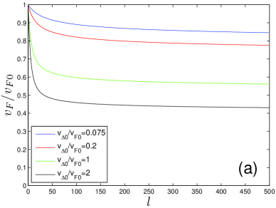
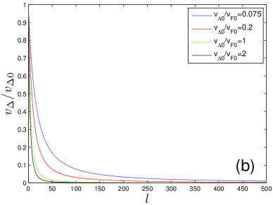
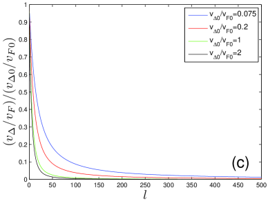
Figure 1: (a), (b), and (c) show how $v_{F}$, $v_{\Delta}$, and $v_{\Delta}/v_{F}$ flow with a varying length scale $l$ respectively in the clean case. The initial values of velocity ratio are $v_{\Delta 0}/v_{F0}=0.075,0.2,1,2$.

However, in the present nodal fermion system, the above two criteria are no longer equivalent. We will show by explicit calculations in this section that the damping rate of nodal fermions vanishes more rapidly than the energy, but the residue $Z_{f}$ vanishes, i.e., $Z_{f}\rightarrow 0$.

3.1 Fermion damping rate and quasiparticle residue

Now we calculate the fermion damping rate and the residue $Z_{f}$ utilizing the solutions of the RG equations (11)-(15). The unusual renormalization of fermion velocities need to be taken into account in an appropriate manner. We only present the results obtained in the clean limit $C_{g}=0$ in this section, and include the effect of random gauge potential in the next section.

After solving RG equations (11)-(13) self-consistently, we show the $l$-dependence of fermion velocities $v_{F}$, $v_{\Delta}$ and ratio $v_{\Delta}/v_{F}$ obtained at different initial values of ratio $v_{\Delta 0}/v_{F0}$ in figures 1(a), (b) and (c) respectively. All the quantities $v_{F}$, $v_{\Delta}$, and $v_{\Delta}/v_{F}$ decrease with growing $l$ and flow eventually to zero as $l\rightarrow+\infty$, but apparently $v_{F}$ decreases much more slowly than $v_{\Delta}$. If we use the ratio $v_{\Delta}/v_{F}$ to characterize the velocity anisotropy, it is clear that the nematic order drives an extreme velocity anisotropy $v_{\Delta}/v_{F}\rightarrow 0$. For later use, it is helpful to extract an approximate analytical expressions for the velocities. Considering the leading and sub-leading terms, the solution for $v_{\Delta}/v_{F}$ is given by

$$\frac{v_{\Delta}}{v_{F}}\sim\frac{\pi^{2}N}{8}\frac{1}{l\ln(c_{s}l)}=\frac{\pi^{2}N}{8}\frac{1}{l\left[\ln(l)+\ln\left(c_{s}\right)\right]},$$ (24)

with $c_{s}\approx 0.3809/N$, which is consistent with the expression in reference [24]. In the long wavelength limit, $l\rightarrow\infty$, $\ln(c_{s})/\ln(l)\rightarrow 0$, so the sub-leading term can be ignored. Retaining only the leading term, the asymptotic behavior of velocity ratio can be well approximated by

$$\frac{v_{\Delta}}{v_{F}}\sim\frac{\pi^{2}N}{8}\frac{1}{l\ln(l)}.$$ (25)

Substituting the asymptotic form of $v_{\Delta}/v_{F}$ into equation (11), we obtain

$$\frac{dv_{F}}{dl}\sim-\frac{\pi^{2}c_{1}}{8}\frac{v_{F}}{l\ln(l)}$$ (26)

with $c_{1}\approx 0.078$ for large $l$. Solving this equation, we express the renormalized $v_{F}$ as

$$v_{F}(l)\sim\frac{1}{(\ln l)^{c_{2}}}$$ (27)

with $c_{2}=\frac{\pi^{2}c_{1}}{8}$. It can also be found that $v_{\Delta}$ at large $l$ behaves approximately as

$$v_{\Delta}(l)\sim\frac{\pi^{2}N}{8}\frac{1}{l\left[\ln(l)\right]^{1+c_{2}}}.$$ (28)

According to equations (27) and (28), both $v_{F}$ and $v_{\Delta}$ vanish as $l\rightarrow+\infty$.

To examine the impact of singular fermion velocity renormalization and extreme velocity anisotropy on the properties of nodal fermions, we will compute a number of physical quantities. Coming first is the quasiparticle residue $Z_{f}$. Apart from the widely used definition given by equation (18), the residue $Z_{f}$ can also be calculated within the RG framework. The interaction induced renormalization of fermion field $\Psi$ is encoded in the residue $Z_{f}$, which exhibits the following $l$-dependence

$$Z_{f}=e^{\int_{0}^{l}\left(C_{1}-C_{g}\right)dl^{\prime}}$$ (29)

or alternatively

$$\frac{dZ_{f}}{dl}=\left(C_{1}-C_{g}\right)Z_{f}.$$ (30)

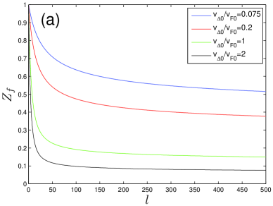
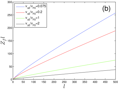
Figure 2: $l$-dependence of $Z_{f}$ in the clean case is presented in (a), and of $Z_{f}l$ in (b). The initial values of velocity ratio are $v_{\Delta 0}/v_{F0}=0.075,0.2,1,2$.

The $l$-dependence of $Z_{f}$ can be easily obtained from the above equation, and is presented in figure 2(a). We find that $Z_{f}$ flows to zero in the limit $l\rightarrow+\infty$, which indicates the breakdown of normal Fermi liquid and the absence of well-defined Landau quasiparticles. However, $Z_{f}$ decreases very slowly with growing $l$, thus the deviation of the system from a normal Fermi liquid ought to be quite weak. To see this point, we plot the $l$-dependence of $Z_{f}l$ in figure 2(b), and find that

$$\lim_{l\rightarrow+\infty}Z_{f}l\rightarrow+\infty.$$ (31)

Therefore, the residue $Z_{f}$ obtained at nematic QCP vanishes with growing $l$ more slowly than that of a MFL [51], where $Z_{f}\sim 1/l$. According to equation (18), one can speculate that

$$\lim_{\omega\rightarrow 0}\frac{\mathrm{Re}\Sigma_{\mathrm{nem}}^{R}(\omega)}{\omega\ln(\omega_{0}/\omega)}\rightarrow 0,$$ (32)

since a large length scale $l$ corresponds to a low energy $\omega$. This speculation in turn implies that the imaginary part of the retarded fermion self-energy $\mathrm{Im}\Sigma_{\mathrm{nem}}^{R}(\omega)$ should display the following low-energy behavior,

$$\lim_{\omega\rightarrow 0}\frac{\mathrm{Im}\Sigma_{\mathrm{nem}}^{R}(\omega)}{\omega}\rightarrow 0.$$ (33)

To make the above discussions more quantitative, we are now going to make a detailed analysis of the asymptotic behavior of $Z_{f}$. At large running scale $l$, the equation of $Z_{f}$ can be approximated by

$$\frac{dZ_{f}}{dl}\sim-\frac{c_{4}}{N}\frac{v_{\Delta}}{v_{F}}Z_{f}\sim-\frac{c_{5}}{l\ln l}Z_{f},$$ (34)

where $c_{4}\approx 0.426$ and $c_{5}=\frac{\pi^{2}c_{4}}{8}\approx 0.523$. Solving this equation leads to the asymptotic behavior

$$Z_{f}\sim\frac{1}{\left(\ln l\right)^{c_{5}}}\rightarrow 0$$ (35)

in the limit $l\rightarrow+\infty$. To proceed, it proves convenient to utilize the relationship between $\omega$ and $l$:

$$\omega=\omega_{\mathrm{0}}e^{-l},$$ (36)

where $\omega_{\mathrm{0}}$ is a cutoff. Then the real part of retarded self-energy is approximated by

$$\mathrm{Re}\Sigma_{\mathrm{nem}}^{R}(\omega) \sim \omega\left\{\ln\left[\ln\left(\frac{\omega_{0}}{\omega}\right)\right]\right\}^{c_{5}}$$ (37)

as $\omega\rightarrow 0$. Using the K.-K. relation, we obtain the imaginary part of self-energy

$$\mathrm{Im}\Sigma_{\mathrm{nem}}^{R}(\omega) \sim \frac{\pi}{2}\frac{|\omega|}{\ln\left(\frac{\omega_{0}}{\omega}\right)\left\{\ln\left[\ln\left(\frac{\omega_{0}}{\omega}\right)\right]\right\}^{1-c_{5}}}.$$ (38)

From equation (38), it is easy to verify that this fermion damping rate is smaller than that in a MFL and manifests the asymptotic behavior $\lim_{\omega\rightarrow 0}\mathrm{Im}\Sigma_{\mathrm{nem}}^{R}(\omega)/\omega\rightarrow 0$, confirming the above analysis based on numerical results. According to the conventional notion of quantum many-body physics, one would expect the system to behave like a normal Fermi liquid. However, in the low energy limit $\omega\rightarrow 0$, the residue $Z_{f}$ actually vanishes:

$$Z_{f}\sim\frac{1}{\left\{\ln\left[\ln\left(\frac{\omega_{0}}{\omega}\right)\right]\right\}^{c_{5}}}\rightarrow 0,$$ (39)

which clearly implies that the system under consideration is actually a non-Fermi liquid and the nodal fermions do not have a well-defined quasiparticle peak in the spectral function. We see that the above residue $Z_{f}$ flows to zero at a lower speed than that of a MFL, i.e., $Z_{f}\sim\frac{1}{\ln(\omega_{0}/\omega)}$. Therefore, the quantum critical fluctuation of nematic order gives rise to an even weaker violation of ordinary Fermi liquid theory than a MFL. To the best of our knowledge, this sort of unconventional non-Fermi liquid state has not been reported previously.

It is now interesting to compare this unconventional non-Fermi liquid state with graphene. In graphene, early perturbative calculations revealed that Dirac fermions exhibit MFL behavior with damping rate $\mathrm{Im}\Sigma^{R}(\omega)\sim\omega$ and vanishing $Z_{f}$ [53]. Nevertheless, subsequent careful RG studies [53, 54, 55, 56] have found that, the fermion damping rate actually depends on energy as $\mathrm{Im}\Sigma^{R}(\omega)\propto\omega/\ln^{2}\omega$ at zero temperature due to the long-range Coulomb interaction, whereas the corresponding $Z_{f}$ flows to a finite value as $\omega\rightarrow 0$. Therefore, graphene is a normal Fermi liquid. In contrast, the massless nodal fermions constitute a non-Fermi liquid at the nematic QCP, because $Z_{f}$ vanishes in the lowest energy limit. The crucial difference between these two cases can be understood as follows. At nematic QCP, the fermion velocities are driven to vanish by the nematic order, so the effective fermion-nematic interaction is significantly pronounced. In graphene, however, the fermion velocity is dramatically enhanced at low energies by Coulomb interaction, which then weakens the effective Coulomb interaction and guarantees the validity of the Fermi liquid description. These two interacting Dirac fermion systems provide interesting new insight on the effects of strong electron correlations and also on the criterion of non-Fermi liquid states.

Moreover, an important lesson one can learn from the research experience of graphene is that, RG may lead to qualitatively different spectral properties of fermions from that obtained by ordinary perturbative expansion approach. Indeed, this is the main motivation that has promoted us to make an extensive RG analysis of the spectral properties of nodal fermions at the nematic QCP.

Figure 3: Fermion DOS $\rho(\omega)$ in the clean limit at different initial values $v_{\Delta 0}/v_{F0}=0.075,0.2,1,2.$

3.2 Density of states and specific heat

We have showed in the last subsection that the nodal fermions exhibit unconventional non-Fermi liquid behaviors at the nematic QCP. In this subsection, we will compute two important quantities, namely DOS and specific heat, on the basis of the RG solutions with the goal to gain a better understanding of the non-Fermi liquid state.

The fermion DOS can calculated from the retarded Green functions of nodal fermions via the definition [25]

$$\rho(\omega) = \sum_{a=1}^{N}\int\frac{dk_{x}dk_{y}}{(2\pi)^{2}}\frac{1}{\pi}\mathrm{Tr}\left[\mathrm{Im}G_{1a}^{R}(v_{F}k_{x},v_{\Delta}k_{y},\omega)+\mathrm{Im}G_{2a}^{R}(v_{F}k_{x},v_{\Delta}k_{y},\omega)\right]$$ (40)

$$= \frac{1}{v_{\Delta}v_{F}}\sum_{a=1}^{N}\int\frac{dk_{x}^{\prime}dk_{y}^{\prime}}{(2\pi)^{2}}\frac{1}{\pi}\mathrm{Tr}\left[\mathrm{Im}G_{1a}^{R}(k_{x}^{\prime},k_{y}^{\prime},\omega)+\mathrm{Im}G_{2a}^{R}(k_{x}^{\prime},k_{y}^{\prime},\omega)\right].$$

In the absence of interactions, the fermion DOS is well-known to be linear in $\omega$, namely $\rho(\omega)\propto\omega$. This linear behavior will be changed once the interaction effects are considered. After including the fermion velocity renormalization, employing the method presented in [25], the flow equation for $\rho(\omega)$ is given by

$$\frac{d\ln\rho}{d\ln\omega} = \left\{\begin{array}[]{ll}\frac{1+C_{1}-C_{2}-C_{3}-C_{g}}{1-C_{1}+C_{2}+C_{g}},&\mathrm{if}\quad v_{\Delta}<v_{F},\\ \\ \frac{1+C_{1}-C_{2}-C_{3}-C_{g}}{1-C_{1}+C_{3}+C_{g}},&\mathrm{if}\quad v_{\Delta}>v_{F}.\end{array}\right.$$ (44)

In cuprates, the initial value of velocity ratio $v_{\Delta 0}/v_{F0}$ is known to be much smaller than $1$ [57]. Additionally, due to the quantum fluctuation of nematic order, $v_{\Delta}/v_{F}$ decreases monotonously as the energy scale is lowering. Therefore, for a given initial value $v_{\Delta 0}/v_{F0}<1$, we only need to consider the case $v_{\Delta}<v_{F}$. In order to show that the conclusion is independent of the condition $v_{\Delta 0}/v_{F0}<1$, we also plot the curves for the case $v_{\Delta 0}/v_{F0}=2$ in figures 3 and 4. The RG equations of DOS and specific heat are also given with a generalized form. In the clean limit, we plot the results for $\rho(\omega)$ in figure 3. We see from figure 3(a) that $\rho(\omega)$ is apparently not linear in $\omega$, but displays the asymptotic behavior

$$\lim_{\omega\rightarrow 0}\frac{\rho(\omega)}{\omega}\rightarrow+\infty.$$ (45)

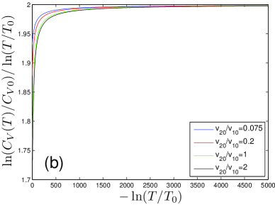
Figure 4: Specific heat $C_{V}(T)$ in the clean limit at different initial values $v_{\Delta 0}/v_{F0}=0.075,0.2,1,2.$

On the other hand, figure 3(b) implies that

$$\lim_{\omega\rightarrow 0}\frac{\ln(\rho(\omega)/\rho_{0})}{\ln(\omega/\omega_{0})}\rightarrow 1.$$ (46)

This DOS $\rho(\omega)$ is qualitatively different from the power law function $\rho(\omega)\sim\omega^{1-\alpha}$, where $\alpha$ is a small finite value, obtained previously in reference [25].

In the non-interacting limit, the fermion specific heat depends on $T$ as $C_{V}(T)\propto T^{2}$. As shown in B, including the influence of the quantum fluctuation of nematic order and random gauge potential leads us to

$$\frac{d\ln C_{V}}{d\ln T} = \left\{\begin{array}[]{ll}2+\frac{2C_{1}-C_{2}-C_{3}-2C_{g}}{1-C_{1}+C_{2}+C_{g}},&\mathrm{if}\quad v_{\Delta}<v_{F},\\ \\ 2+\frac{2C_{1}-C_{2}-C_{3}-2C_{g}}{1-C_{1}+C_{3}+C_{g}},&\mathrm{if}\quad v_{\Delta}>v_{F}.\end{array}\right.$$ (50)

At low $T$, $C_{V}(T)$ behaves as

$$\lim_{T\rightarrow 0}\frac{C_{V}(T)}{T^{2}}\rightarrow+\infty,$$ (51)

which is visualized in figure 4(a). Apparently, the original quadratic $T$-dependence of $C_{V}(T)$ obtained in the non-interacting limit is significantly altered. According to figure 4(b), we can express $C_{V}(T)$ at very small $T$ as

$$\lim_{T\rightarrow 0}\frac{\ln(C_{V}(T)/C_{V0})}{\ln(T/T_{0})}\rightarrow 2,$$ (52)

which is also distinct from the power law $T$-dependence $C_{V}(T)\sim T^{2-\beta}$, where $\beta$ is a small finite constant, obtained previously [25].

Simple analysis reveal that the three parameters $C_{1}$, $C_{2}$, and $C_{3}$ appearing in the RG equations (44) and (50) all flow to zero in the lowest energy limit [24]. This asymptotic behavior makes it impossible to express $\rho(\omega)$ and $C_{V}(T)$ by power law functions. As given in C, the low energy behavior of $\rho(\omega)$ and the low-$T$ behavior of $C_{V}(T)$ can be approximately expressed as

$$\rho(\omega) \sim \left(\frac{\omega}{\omega_{0}}\right)\ln\left(\frac{\omega_{0}}{\omega}\right)\left(\ln\ln\left(\frac{\omega_{0}}{\omega}\right)\right)^{a_{\rho}}\exp\left[\frac{1}{2}\left(\ln\ln\ln\left(\frac{\omega_{0}}{\omega}\right)\right)^{2}\right],$$ (53)

$$C_{V}(T) \sim \left(\frac{T}{T_{0}}\right)^{2}\ln\left(\frac{T_{0}}{T}\right)\left(\ln\ln\left(\frac{T_{0}}{T}\right)\right)^{a_{C}}\exp\left[\frac{1}{2}\left(\ln\ln\ln\left(\frac{T_{0}}{T}\right)\right)^{2}\right],$$ (54)

where $a_{\rho}$ and $a_{C}$ are two negative constants. At $N=2$, $a_{\rho}\approx-1.896$ and $a_{C}\approx-1.466$.

We notice that our RG equation for $C_{V}(T)$ (50) is not exactly the same as that obtained by Xu et al. [25]. This difference does not affect our conclusion that $C_{V}(T)$ is not a power law function at low $T$. Indeed, if we start from the RG equation of $C_{V}(T)$ presented in [25], we reach the same conclusion. A more detailed discussion is presented in B and C.

4 Impact of Random gauge potential

In this section, we investigate the impact of random gauge potential on the quantum critical behaviors near the nematic QCP. We will first show the RG solutions obtained in the presence of random gauge potential, and then re-calculate the fermion DOS and specific heat after considering the influence of disorder scattering. To this end, we need to retain a nonzero $C_{g}$ in the RG equations (11)-(15), (30), (44), and (50), and then solve these RG equations numerically.

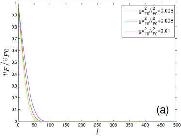
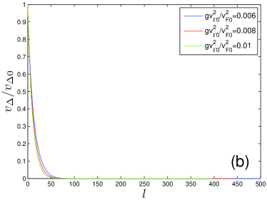
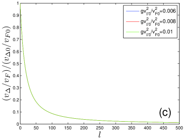
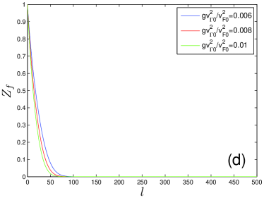
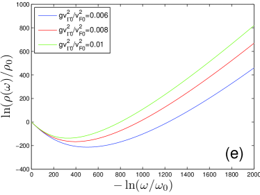
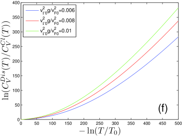
Figure 5: Flows of the quantities $v_{F}$, $v_{\Delta}$, $v_{\Delta/v_{F}}$, $Z_{f}$, $\rho$, $C_{V}$ are shown in (a), (b), (c), (d), (e), and (f) respectively at the initial value $v_{\Delta 0}/v_{F0}=0.075$ in the presence of random gauge potential. We have chosen $v_{\Gamma 0}^{2}g/v_{F0}^{2}=0,006,0.008,0.01$ and $v_{\Gamma 10}=v_{\Gamma 20}=v_{\Gamma 0}$ for random gauge potential.

4.1 Flow of effective disorder strength

In order to make a direct comparison to the clean case in which $C_{g}=0$ and to explicitly see the influence of a nonzero $C_{g}$ on the running behaviors of various parameters, we plot the $l$-dependence of $v_{F}$, $v_{\Delta}$, $v_{\Delta}/v_{F}$, and $Z_{f}$ in figures 5(a)-(d). Moreover, we show the $\omega$-dependence of $\rho(\omega)$ in figure 5(e) and the $T$-dependence of $C_{V}$ in figure 5(f), respectively. We will discuss under what circumstances these RG results are modified in the next subsection.

Comparing figures 3(a) and (b) with figures 5(a) and (b), we see that the detailed $l$-dependence of $v_{F}$ and $v_{\Delta}$ are both altered dramatically by the random gauge potential. As shown in figure 3(c) and figure 5(c), the velocity ratio $v_{\Delta}/v_{F}$ exhibits exactly the same $l$-dependence in the clean and disordered cases, which originates from the fact that $C_{g}$ does not enter into the RG equation of velocity ratio $v_{\Delta}/v_{F}$. According to figure 2(a) and figure 5(d), the renormalization factor $Z_{f}$ flows to zero in the disordered case much more rapidly than the clean case.

As shown in figure 5(e), the DOS $\rho(\omega)$ is divergent in the lowest energy limit due to random gauge potential. This is completely different from the behaviors of clean case presented in figure 3. In figure 5(f), we plot the ratio between $C_{V}^{\mathrm{Dis}}/C_{V}^{\mathrm{Cl}}$, where $C_{V}^{\mathrm{Dis}}$ and $C_{V}^{\mathrm{Cl}}$ are the specific heat obtained in disordered and clean cases, respectively. Since the solutions of the RG equations about DOS and specific heat are modified substantially in the disordered case, it turns out that random gauge potential is a relevant perturbation in the present system. To verify the relevance of random gauge potential, we should appeal to the RG analysis of the effective disorder strength.

In the action term $S_{\mathrm{dis}}$ given in equation (4), the parameters that characterize the fermion-disorder coupling seem to be $v_{\Gamma 1}$ and $v_{\Gamma 2}$. It can be seen from the RG equations that $v_{\Gamma 1}$ flows in precisely the same way as $v_{F}$, and that $v_{\Gamma 2}$ as $v_{\Delta}$. Thus, both $v_{\Gamma 1}$ and $v_{\Gamma 2}$ are strongly renormalized and driven to vanish as $l\rightarrow+\infty$. However, this does not mean that the disorders can be simply neglected. Indeed, whether disorders are important is determined by the ratio between the interaction energy given by $S_{\mathrm{dis}}$ and the fermion energy $E_{k}\propto\left(v_{F}^{2}k_{x}^{2}+v_{\Delta}^{2}k_{y}^{2}\right)^{1/2}$. We can see that this ratio is defined by $C_{g}$, which enters into the RG equations for the parameters $v_{F}$, $v_{\Delta}$, $v_{\Gamma 1}$, and $v_{\Gamma 2}$. The effective strength of random gauge potential should be measured by $C_{g}$, rather than $v_{\Gamma 1}$ and $v_{\Gamma 2}$. Recall that $C_{g}$ is a function of five parameters, i.e., $v_{F}$, $v_{\Delta}$, $v_{\Gamma 1}$, $v_{\Gamma 2}$, and $g$. Among these parameters, $g$ is assumed to be a dimensionless constant, but the other four parameters flow strongly with the varying $l$. Detailed RG analysis revealed that $C_{g}$ goes to infinity, namely

$$C_{g} = \frac{g}{2\pi}\left(\frac{v_{\Gamma 10}^{2}}{v_{F0}^{2}}\frac{v_{F}}{v_{\Delta}}+\frac{v_{\Gamma 20}^{2}}{v_{\Delta 0}^{2}}\frac{v_{\Delta}}{v_{F}}\right)\rightarrow+\infty,$$ (55)

in the limit $l\rightarrow+\infty$ as a consequence of the singular renormalization of the fermion velocities ratio $v_{\Delta}/v_{F}$. More quantitatively, the large scale behavior of $C_{g}$ can be described by

$$C_{g}\sim c_{3}l\ln l,$$ (56)

where $c_{3}=\frac{4g}{\pi^{3}N}\frac{v_{\Gamma 10}^{2}}{v_{F0}^{2}}$.

It is necessary to explain here why the effective strength of random gauge potential should be represented by $C_{g}$, rather than solely by the coefficients $v_{\Gamma i}$ with $i=1,2$, and why $C_{g}\rightarrow\infty$ in the lowest energy limit. In an interacting fermion system, the effective strength of the interaction is characterized by the ratio between the interaction energy scale and the kinetic energy of fermions. This ratio is widely used in condensed matter physics to judge whether an interacting fermion system can be defined as a strongly correlated system or not. For instance, the normal metal with a high density of itinerant electrons is believed to be a weakly interacting system since the energy scale of Coulomb potential is much smaller than the Fermi energy. In a massless Dirac fermion system (such as graphene), the effective strength of long-range Coulomb interaction is defined as $\alpha\sim\frac{e^{2}}{v_{F}}$, where $e^{2}$ appears in the action of the Coulomb interaction as a coupling coefficient and the fermion velocity $v_{F}$ reflects the order of the kinetic energy [54, 56]. Another example comes from the effective BCS model of Dirac fermion systems, where the effective strength of pairing interaction is characterized by $g\sim\frac{u}{v_{F}}$ with $u$ being the coupling coefficient of pairing interaction and $v_{F}$ fermion velocity [58, 59].

This criterion also applies to disordered systems. When massless Dirac fermions couple to random gauge potential, the effective strength of random gauge potential should be defined by $C_{g}\sim\frac{v_{\Gamma i}^{2}}{v_{F}v_{\Delta}}$, rather than the coefficient of fermion-disorder coupling $v_{\Gamma i}$ [47, 48]. When $v_{\Gamma i}$ flows to zero in the lowest energy limit, $C_{g}$ does not necessarily vanish since there is a possibility that $v_{F}$ and $v_{\Delta}$ may vanish more (or equally) rapidly than $v_{\Gamma i}$. When the nodal fermions couple to both the quantum fluctuation of nematic order and random gauge potential, the four parameters $v_{F}$, $v_{\Delta}$, $v_{\Gamma 1}$, and $v_{\Gamma 2}$ all flow to zero in the lowest energy limit, but the effective strength of random gauge potential becomes very large, namely $C_{g}\rightarrow\infty$. This originates from the fact that $\frac{v_{\Gamma 1}}{v_{F}}=\frac{v_{\Gamma 10}}{v_{\Gamma 20}}$ and $\frac{v_{\Gamma 2}}{v_{\Delta}}=\frac{v_{\Gamma 20}}{v_{\Delta 0}}$ are constants, while at the same time the velocity ratio $v_{\Delta}/v_{F}\rightarrow 0$. The behavior $C_{g}\rightarrow\infty$ at low energies indicates that random gauge potential is relevant. To see this point, we neglect the nematic order and consider only the coupling of nodal fermions to random gauge potential, which results in simplified RG equations:

$$\frac{dv_{F}}{dl}=-C_{g}v_{F},\,\frac{dv_{\Delta}}{dl}=-C_{g}v_{F},\,\frac{d(v_{F}/\Delta)}{dl}=0,\,\frac{dv_{\Gamma 1}}{dl}=-C_{g}v_{F},\,\frac{dv_{\Gamma 2}}{dl}=-C_{g}v_{F}.$$ (57)

Using the two relations $\frac{v_{\Gamma 1}}{v_{F}}=\frac{v_{\Gamma 10}}{v_{\Gamma 20}}$ and $\frac{v_{\Gamma 2}}{v_{\Delta}}=\frac{v_{\Gamma 20}}{v_{\Delta 0}}$, it is easy to show that

$$C_{g}=\frac{g}{2\pi}\frac{v_{\Gamma 1}^{2}+v_{\Gamma 2}^{2}}{v_{F}v_{\Delta}}=\frac{g}{2\pi}\frac{v_{\Gamma 10}^{2}+v_{\Gamma 20}^{2}}{v_{F0}v_{\Delta 0}}=C_{g0}.$$ (58)

In this case, $v_{F}$, $v_{\Delta}$, $v_{\Gamma 1}$, and $v_{\Gamma 2}$ depend on length scale $l$ as

$$\frac{v_{F}}{v_{F0}}=\frac{v_{\Delta}}{v_{\Delta 0}}=\frac{v_{\Gamma 1}}{v_{\Gamma 10}}=\frac{v_{\Gamma 2}}{v_{\Gamma 20}}=e^{-C_{g0}l},$$ (59)

which all vanish rapidly in the limit $l\rightarrow\infty$. Since $C_{g}$ is a constant, random gauge potential is marginal. From the above calculations, we can conclude that the behavior $C_{g}\rightarrow\infty$ obtained in the presence of both nematic fluctuation and random gauge potential is directly related to the extreme velocity anisotropy $v_{\Delta}/v_{F}\rightarrow 0$ induced by the quantum fluctuation of nematic order. The flow of $C_{g}$ towards strong coupling regime is a clear signature that random gauge potential should have substantial physical effects on the low-energy behaviors of nodal fermions, which will be discussed in the next subsection.

We notice other interesting correlated electron models in which the coupling coefficient of an interaction vanishes at low energies, but the interaction is not negligible due to the more (or equally) rapid decrease of the kinetic energy of electrons. Recently, Sur and Lee studied the influence of quantum fluctuations of an antiferromagnetic (AF) order at an AF quantum critical point in a metal supporting one-dimensional Fermi surface [60]. In particular, they showed that the coupling coefficient of the interaction flows to zero at low energies. However, the fermion velocity also vanishes, thus the interaction cannot be simply neglected. Actually, Sur and Lee found that the interaction drives the system to become a so-called quasi-local strange metal that is apparently qualitatively different from the free fermion system.

4.2 Physical effects of random gauge potential

How should we understand the divergence of $C_{g}$? In order to answer this question, we first consider the non-interacting system that contains only nodal fermions and random gauge potential. In this case, the RG equation of fermion DOS becomes

$$\frac{d\ln\rho}{d\ln\omega}=\frac{1-C_{g0}}{1+C_{g0}},$$ (60)

with

$$C_{g0}=\frac{g}{2\pi}\frac{v_{\Gamma 10}^{2}+v_{\Gamma 20}^{2}}{v_{F0}v_{\Delta 0}}.$$ (61)

If $C_{g0}<1$, we have

$$\rho(\omega)\sim\omega^{\alpha}\quad\mathrm{with}\quad\alpha=\frac{1-C_{g0}}{1+C_{g0}},$$ (62)

where $\alpha$ satisfies $0<\alpha<1$. In this case, the RG equation for specific heat is given by

$$\frac{d\ln C_{V}}{d\ln T}=2-\frac{2C_{g0}}{1+C_{g0}}.$$ (63)

The solution of this equation is given by

$$C_{V}(T)\sim T^{\beta}\quad\mathrm{with}\quad\beta=2-\frac{2C_{g0}}{1+C_{g0}}.$$ (64)

If $C_{g}>1$, it is easy to get

$$\rho(\omega)\rightarrow\infty$$ (65)

in the limit $\omega\rightarrow 0$. The divergence $\rho(\omega)$ indicates the emergence of a disorder dominated diffusive state, in which a finite disorder scattering rate $\gamma$ and a finite zero-energy DOS $\rho(0)$ are generated [49, 61, 62]. The value $C_{g}=1$ defines a QCP for the quantum phase transition between the ballistic and diffusive states of nodal fermions. Therefore, a weak random gauge potential gives rise to power law behavior of $\rho(\omega)$, whereas a sufficiently strong disorder can trigger the quantum phase transition to a diffusive state.

In the presence of both nematic critical fluctuation and random gauge potential, the fact that $C_{g}\rightarrow\infty$ in the lowest energy limit signals the development of a disorder dominated diffusive state and the generation of a finite $\gamma$ and a finite $\rho(0)$ even in the case of weak random gauge potential. Although the perturbative RG method provides a powerful tool to judge whether and when a phase transition takes place, it cannot be used to compute the precise value of $\gamma$. To calculate $\gamma$, one usually needs to construct a self-consistent equation for the retarded fermion self-energy by properly considering both the fermion-disorder scattering and the influence of quantum critical fluctuation of nematic order [66]. This is an interesting yet complicated issue, which is beyond the scope of the present work and subjected to future research. Here, we use the RG method to make a rough estimation for the energy scale of $\gamma$. As shown in Fig. 5(e), for small given values of $C_{g0}$ and $v_{\Delta 0}/v_{F0}$, the solution of the RG equation of DOS should have the following properties: $\rho(\omega)$ decreases as the varying energy scale decreases, but tends to increase when the energy scale exceeds a critical value $E_{c}(C_{g0},v_{\Delta 0}/v_{F0})$, which is a function of $C_{g0}$ and $v_{\Delta 0}/v_{F0}$. The magnitude of $\gamma$ should be an increasing function of $E_{c}$. In the following calculations of $\rho(0)$ and $C_{V}(T)$, we will regard $\gamma$ as an undetermined constant. Fortunately, the qualitative behaviors of $\rho(0)$ and $C_{V}(T)$ in the low energy regime is independent of the precise value of $\gamma$.

The imaginary part of retarded fermion self-energy can be generically written as

$$\mathrm{Im}\Sigma^{R}(\omega)\approx\gamma+\mathrm{Im}\Sigma_{\mathrm{nem}}^{R}(\omega),$$ (66)

where $\mathrm{Im}\Sigma_{\mathrm{nem}}^{R}(\omega)$ is the contribution induced solely by the nematic order. The disorder-induced scattering rate $\gamma$ represents a characteristic energy scale. At energies higher than $\gamma$, namely $\omega>\gamma$, $\mathrm{Im}\Sigma_{\mathrm{nem}}^{R}(\omega)$ dominates over $\gamma$ and all the RG results for $v_{F}$, $v_{\Delta}$, $Z_{f}$, $\rho(\omega)$, and $C_{V}(T)$ shown in figures 5(a)-(f) are still applicable. At $\omega<\gamma$, the diffusive motion of nodal fermions and its interplay with critical nematic fluctuation govern the low-energy properties of the system.

Once a finite $\gamma$ is generated, the renormalized velocities $v_{F}$ and $v_{\Delta}$ no more vanish at low energies, which is apparently different from the clean case. Instead, as the energy scale decreases, both $v_{F}$ and $v_{\Delta}$ are saturated to certain finite values, denoted by $v_{F0}^{\prime}$ and $v_{\Delta 0}^{\prime}$, below the energy scale set by $\gamma$. Hence, there is no extreme velocity anisotropy in the diffusive state. The fermion DOS and specific heat also exhibit different behaviors comparing to the clean case. To demonstrate the difference in DOS, we write the retarded propagators of nodal fermions in the forms:

$$G_{1a}^{R}(\omega,\mathbf{k}) = \frac{1}{-(\omega+i\gamma)+v_{F0}^{\prime}k_{x}\tau^{z}+v_{\Delta 0}^{\prime}k_{y}\tau^{x}},$$ (67)

$$G_{2a}^{R}(\omega,\mathbf{k}) = \frac{1}{-(\omega+i\gamma)+v_{F0}^{\prime}k_{y}\tau^{z}+v_{\Delta 0}^{\prime}k_{x}\tau^{x}}.$$ (68)

Calculations find that the fermion DOS depends on $\omega$ as

$$\rho(\omega) = \frac{N\gamma}{2\pi v_{F0}^{\prime}v_{\Delta 0}^{\prime}}\left[\ln\left(\frac{\left(\gamma^{2}-\omega^{2}+v_{F0}^{\prime}v_{\Delta 0}^{\prime}\Lambda^{2}\right)^{2}+4\omega^{2}\gamma^{2}}{\left(\gamma^{2}-\omega^{2}\right)^{2}+4\omega^{2}\gamma^{2}}\right)\right.$$ (69)

$$\left.+\frac{2\omega}{\gamma}\arctan\left(\frac{\gamma^{2}-\omega^{2}+v_{F0}^{\prime}v_{\Delta 0}^{\prime}\Lambda^{2}}{2\omega\gamma}\right)-\frac{2\omega}{\gamma}\arctan\left(\frac{\gamma^{2}-\omega^{2}}{2\omega\gamma}\right)\right].$$

In the case $\sqrt{v_{F0}^{\prime}v_{\Delta 0}^{\prime}}\Lambda\gg\gamma$, we have

$$\rho(0)\approx \frac{2N\gamma}{\pi v_{F0}^{\prime}v_{\Delta 0}^{\prime}}\ln\left(\frac{\sqrt{v_{F0}^{\prime}v_{\Delta 0}^{\prime}}\Lambda}{\gamma}\right).$$ (70)

In order to compute the specific heat, it is convenient to invoke the standard Matsubara formalism of fermion propagators, i.e.,

$$G_{1a}(\omega_{n},\mathbf{k}) = \frac{1}{-i(\omega_{n}+\gamma\mathrm{sgn}(\omega_{n}))+v_{F0}^{\prime}k_{x}\tau^{z}+v_{\Delta 0}^{\prime}k_{y}\tau^{x}},$$

$$G_{2a}(\omega_{n},\mathbf{k}) = \frac{1}{-i(\omega_{n}+\gamma\mathrm{sgn}(\omega_{n}))+v_{F0}^{\prime}k_{y}\tau^{z}+v_{\Delta 0}^{\prime}k_{x}\tau^{x}},$$

where $\omega_{n}=(2n+1)\pi T$ with $n$ being integer. The fermion free energy is given by

$$F=-\frac{2NT}{v_{F0}^{\prime}v_{\Delta 0}^{\prime}}\sum_{\omega_{n}}\int\frac{d^{2}k}{(2\pi)^{2}}\ln\left[\left(\omega_{n}+\gamma\mathrm{sgn}(\omega_{n})\right)^{2}+k^{2}\right].$$

Summing over $\omega_{n}$ leads to

$$F \approx -\frac{4N}{\pi v_{F0}^{\prime}v_{\Delta 0}^{\prime}}\int\frac{d^{2}k}{(2\pi)^{2}}\left\{k\arctan\left(\frac{k}{\pi T+\gamma}\right)+\frac{\gamma}{2}\ln\left[\left(\pi T+\gamma\right)^{2}+k^{2}\right]\right\}.$$ (71)

Now the fermion specific heat in the low energy regime can be approximately given by

$$C_{V} \approx \frac{6NT}{v_{F0}^{\prime}v_{\Delta 0}^{\prime}}\gamma\ln\left(\frac{\Lambda}{\gamma}\right),$$ (72)

which depends on $T$ linearly. We can see that DOS and specific heat obtained in the diffusive state exhibit entirely different behaviors from the unconventional non-Fermi liquid state below the energy scale $\gamma$.

We finally make a brief remark on the behavior of the system staying away from the nematic QCP. Suppose the system stays at a distance $r$ to the QCP, the RG results are still valid and the fermion velocity ratio is still renormalized at energies higher than the scale corresponding to $r$. However, the renormalization terminates at certain low energy scale. Therefore, the effective strength of random gauge potential is moderately enhanced compared its bare value, though $C_{g}$ does not diverge.

5 Comparison with experiments

In this section, we address the possible connection between the theoretical results obtained in the last sections and the phenomenology of cuprate superconductors. We are particularly interested in three existing experimental findings about some of the unusual properties of the superconducting dome.

5.1 Anomalous residual linear-$T$ term of specific heat in cuprates

We first discuss the residual specific heat in cuprates. Due to the line nodes of $d$-wave gap, the specific heat in the superconducting phase of cuprates is expected to exhibit a $T^{2}$ behavior, i.e., $C_{V}(T)\propto T^{2}$, at low $T$. This expectation is generically consistent with experiments [67]. In the lowest $T$ limit, experiments have observed a residual linear $T$ term of $C_{V}(T)$ [67, 68, 69, 70], which is usually attributed to the finite fermion DOS generated by disorder scattering and is also well consistent with the result given by equation (72). There is, however, an unexpected experimental finding [67, 70] that the residual specific heat of YBCO is obviously larger in magnitude than that of La_2-xSr_xCuO₄ (LSCO), although the former material is known to be cleaner than the latter. Apparently, disorder scattering alone is not capable of accounting for this experimental fact. Recently, coexistence of $d$-wave superconductivity with a loop current order was proposed to give a possible explanation [71, 72, 73] for the large residual linear-$T$ term of specific heat in YBCO. In this scenario, when $d$-wave superconductivity coexists with a loop current order, two of four nodal points are converted to finite Fermi pockets of Bougoliubov quasiparticles, which then generates a finite $\rho(0)$ and a residual linear-$T$ term of specific heat [71, 72, 73, 74]. The recent ultrasound measurements showed the possible evidence for the existence of loop current order in YBCO[75, 76].

Here we propose an alternative explanation for the above anomalous experimental results of residual specific heat. Our RG analysis found that the effective strength of random gauge potential, being the most relevant disorder to cuprates [48], is strongly enhanced by the critical nematic fluctuation, which in turn increases the residual value of the specific heat. To understand the role of quantum nematic fluctuation, we firstly consider only the coupling of nodal fermions to random gauge potential. In this special case, $C_{g}$ does not flow and thus remains a constant, namely $C_{g}=C_{g0}$. If $C_{g0}$ is very small, which means the system is only slightly disordered, the behavior of $\rho(\omega)$ and specific heat would be governed by equations (62) and (64), respectively. In this case, the system does not develop a finite $\rho(0)$ and there is no residual liner-$T$ term of specific heat. If the system is quite disordered such that $C_{g0}>1$, it enters a diffusive state with a finite scattering rate $\gamma$, which induces a finite $\rho(0)$ and a residual linear-$T$ term of specific heat. Apparently, the residual specific heat is larger in more disordered systems, which is not consistent with the aforementioned experiments of residual specific heat. If we consider both the quantum fluctuation of nematic order and random gauge potential, $C_{g}$ is significantly enhanced and flows to strong coupling at low energies even if $C_{g0}$ takes an arbitrarily small value. This implies that a cleaner compound might acquire a larger amount of $\gamma$ and naturally a larger $\rho(0)$.

To make a more careful comparison between theories and experiments, we now briefly discuss the doping dependence of our results. We use $\delta$ to denote the doping concentration and $\delta_{c}$ the nematic QCP. At zero temperature, the mass of nematic field $\phi$ is proportional to the difference between $\delta$ and $\delta_{c}$, namely $r\sim|\delta-\delta_{c}|$. When the cuprate is at a distance $r$ away from the nematic QCP, the quantum fluctuation of nematic order is not critical, but remains important for small $r$. At the energy scales larger than $r$, the fermion velocity anisotropy is still considerably enhanced, which leads $C_{g}$ to flow to larger values. For a given small value of $C_{g0}$, $C_{g}$ can flow to a sufficiently large value to induce a diffusive state and generate a finite scattering rate $\gamma$, provided that $r$ is made sufficiently small. In this case, the quantum fluctuation of nematic order can result in a finite $\rho(0)$ and a finite residual linear-$T$ term of specific heat. If the bare value $C_{g0}$ is large enough, random gauge potential itself suffices to generate a finite $\gamma$. Including the quantum fluctuation of nematic order leads to larger values of both $C_{g}$ and $\gamma$. In any case, the quantum fluctuation of nematic order tends to amplify $\gamma$, which naturally increase $\rho(0)$ and the residual specific heat.

A number of recent experiments provided strong evidence supporting the existence of nematic order in YBCO, whereas there is little evidence for nematicity in LSCO. Although YBCO is cleaner than LSCO, the quantum fluctuation of nematic order in the former superconductor can drive $C_{g}$ to flow to much larger values. As a consequence, the residual linear-in-$T$ term of specific heat of YBCO would be larger than that of LSCO. We emphasize that, disorder itself cannot explain the anomalous behaviors of the residual specific heat observed in YBCO and LSCO, and it is necessary to consider the interplay of quantum nematic fluctuation and random gauge potential.

For the above elaboration, we know that the roles played by the quantum nematic fluctuation and random gauge potential depends on doping $\delta$. To simplify discussion, we assume the bare value $C_{g0}$ displays only a weak $\delta$-dependence. Since the quantum fluctuation of nematic order is most pronounced at the nematic QCP, the scattering rate $\gamma$ and consequently the coefficient of the residual liner-$T$ term of specific heat are maximal at the QCP, and decrease as the system moves away from this QCP. This doping dependence is observable, and can be examined by experiments. Within the loop current order scenario, both the zero-energy DOS $\rho(0)$ and the residual linear-$T$ term of specific heat are proportional to the order parameter of the loop current order, which decreases with the growing doping in the underdoped region.

Early experiments [67, 68, 69] found that the coefficient of linear-$T$ term of specific heat at optimally doped YBCO is roughly $2$ mJ$\cdot$mol^-1$\cdot$K^-2. More recent measurements performed in underdoped YBCO [70] revealed that this coefficient is $1.85\pm 0.06$ mJ$\cdot$mol^-1$\cdot$K^-2. We feel that the currently available experimental data about the doping dependence of this coefficient are still quite limited. We expect more extensive measurements would be performed in the future to extract a more quantitative doping dependence of the coefficient, which could help to judge whether the scenario proposed in this paper works.

5.2 Strong damping rate of nodal fermions in optimally doped BSCCO

We next apply the RG results to understand the observed damping rate of nodal fermions in cuprates. Valla et al. [77] have performed extensive angle resolved photoemission spectroscopy measurements in optimally doped Bi₂Sr₂CaCu₂O_8+δ (BSCCO). Their main discovery is that the nodal fermions exhibit a MFL-type damping rate in the normal state above $T_{c}$, which is in general consistency with the observed linear resistivity. They further found [77] that the linear damping rate is not sensitive to the onset of superconductivity and persists well below $T_{c}$. This was out of expectation since previous BCS weak coupling analysis [1, 78] had predicted a quite weak damping rate, i.e., $\mathrm{Im}\Sigma^{R}(\omega,T)\propto\max(\omega^{3},T^{3})$, in the superconducting phase. Several scenarios [1, 20, 79] were proposed to account for the nearly MFL behavior. In particular, Vojta et al. [20] and Khveshchenko and Paaske [79] have argued that the strong fermion damping may arise from a secondary phase transition from a $d_{x^{2}-y^{2}}$-wave superconducting state to a $d_{x^{2}-y^{2}}+is$ or $d_{x^{2}-y^{2}}+id_{xy}$-wave superconducting state.

Experimentally, the existence of a nematic phase was observed in BSCCO by Lawler et al. [13]. More recent experimental studies of Fujita et al. provided further evidence pointing towards the existence of a nematic QCP in the vicinity of optimal doping in BSCCO [14, 19]. Therefore, it seems natural to account for the experimental finding of Valla et al. by considering the quantum critical fluctuation of nematic order. We have showed through RG analysis that the nodal fermion damping rate caused by critical nematic fluctuation, described by $\mathrm{Im}\Sigma_{\mathrm{nem}}^{R}(\omega)$, is slightly weaker than that of a MFL. In realistic experiments, it is difficult to distinguish this non-Fermi liquid state from a MFL state. Therefore, presence of a nematic QCP provides an alternative scenario for the nearly MFL behavior observed in optimally doped BSCCO. However, the nearly MFL behavior occurs only at energies higher than the value $\omega_{\gamma}$ set by disorder scattering rate $\gamma$. Indeed, at $\omega<\omega_{\gamma}$, $\gamma$ dominates over $\mathrm{Im}\Sigma_{\mathrm{nem}}^{R}(\omega)$, thus a finite zero-energy DOS $\rho(0)$ is generated. To summarize, our RG results are qualitatively consistent with the quasiparticle self-energy $\mathrm{Im}\Sigma(\omega,T)=\gamma+\max(\omega,T)$ observed in reference [77].

5.3 Temperature dependence of fermion velocity in BSCCO

Another experiment is the observation of Plumb et al. [80] that the fermion velocity $v_{F}$ along the nodal directions increases as $T$ grows in BSCCO. We know from RG results that the critical nematic fluctuations drive the fermion velocities to vanish in the lowest energy limit. This means the velocities must increase as the energy scale is growing. Therefore, the nematic quantum fluctuation will induce increment of fermion velocities when the thermal energy increases with growing $T$, which is qualitatively well consistent with the observation of Plumb et al. Technically, one can translate the $l$-dependence of fermion velocity to a $T$-dependence by making the transformation $T=T_{0}e^{-l}$ [31, 81]. With the help of this transformation, it is easy to show that the fermion velocity $v_{F}$ is an increasing function of $T$. Therefore, the singular renormalization of fermion velocities of nodal fermions induced by the quantum fluctuation of namatic order, which is first discovered by Huh and Sachdev [24], agrees with the $T$-dependence of $v_{F}$ observed in reference [80].

6 Summary and discussions

In summary, we have found that the nodal fermions of $d$-wave superconductors constitute an unconventional non-Fermi liquid, which exhibits a weaker violation of Fermi liquid description than a MFL, due to the quantum critical fluctuation of nematic order. This unusual state represents a novel quantum state of matter that cannot be well captured by the traditional classification of (non-) Fermi liquids and thus enriches our knowledge of strong electron correlation effects. We also have calculated the fermion DOS and specific heat after incorporating the unusual renormalization of fermion velocities. When a gauge-potential-type disorder is added to the system, we have analyzed its interplay with the quantum fluctuation of nematic order, and found that the effective disorder strength flows to strong coupling, leading to diffusive motion of nodal fermions. Therefore, even a weak random gauge potential can drive a quantum phase transition from a unconventional non-Fermi liquid state to a disorder dominated diffusive state. However, the unusual fermion damping induced by the nematic order is more important than the disorder scattering at high temperatures, where the nodal fermions still display the unconventional non-Fermi liquid behaviors. We finally have discussed the connection between our theoretic results and a number of interesting experiments in the context of some cuprate superconductors.

We now would like compare our work to the existing extensive works on the non-Fermi liquid behaviors in two-dimensional metals produced by the quantum critical fluctuation of nematic order. At the QCP of Pomeranchuk instability in two-dimensional metals, the quantum fluctuation of nematic order can lead to very strong fermion damping [36, 82, 83, 84, 85, 86]. To the leading order, it is found [36, 82, 83, 84, 85, 86] the fermion damping rate behaves as $\mathrm{Im}\Sigma(\omega)\sim\omega^{2/3}$ and the quasiparticle residue $Z_{f}\sim\omega^{1/3}$. Since $Z_{f}$ vanishes in the limit $\omega\rightarrow 0$, this QCP exhibits non-Fermi liquid behavior. In this paper, we have considered the interaction between the quantum fluctuation of nematic order and massless nodal fermions in the superconducting dome of cuprate superconductors. It is apparent that the quantum critical fluctuation of nematic order gives rise to a stronger fermion damping effect in metals than in the superconducting dome of cuprates. This difference should be owing to the different forms of the kinetic energies of fermionic excitations. In the context of cuprates, the kinetic energy of the massless Dirac fermions excited from the superconducting gap nodes is $E=\sqrt{v_{F}^{2}k_{x}^{2}+v_{\Delta}^{2}k_{y}^{2}}$. In contrast, in a two-dimensional metal with a finite Fermi surface, the kinetic energy of fermions can be written as $E=v_{F}k_{x}+\frac{k_{y}^{2}}{2m}$, where $k_{x}$ is the momentum component perpendicular to the Fermi surface and $k_{y}$ is the momentum component along the tangential direction [36, 82, 83, 84, 85, 86]. In the low-energy regime, the latter kinetic energy is smaller that the former for the same given values of momenta, which indicates that the interaction plays a more important role in the latter system than the former. To further demonstrate this difference, we consider the different roles of the long-range Coulomb interaction in a two-dimensional Dirac semimetal and a two-dimensional semi-Dirac semimetal. In a Dirac semimetal, the kinetic energy of Dirac fermions is simply $E=v_{F}k$ with $k=\sqrt{k_{x}^{2}+k_{y}^{2}}$. RG analysis showed that the residue $Z_{f}$ approaches a finite value at low energies, so the system is a normal Fermi liquid[52, 53, 54, 55, 56]. In a semi-Dirac semimetal, the kinetic energy of fermions is written as $E=\sqrt{v_{F}^{2}k_{x}^{2}+\frac{k_{y}^{2}}{4m^{2}}}$ [87, 88]. In this case, the long-range Coulomb interaction drives $Z_{f}$ to vanish in the lowest energy limit, i.e., $Z_{f}\rightarrow 0$, which apparently implies the breakdown of Fermi liquid behavior [87]. Once again, we see that the ratio between the interaction energy scale and the kinetic energy is a crucial quantity to determine the low-energy behaviors of an interacting fermion system.

The coupling of nodal fermions to the quantum fluctuation of antiferromagnetic (AF) order is also an interesting problem [7, 89]. Uemura [7] considered the coupling of nodal fermions to the $(\pi,\pi)$ AF fluctuation, and suggested a possibility that the $(\pi,\pi)$ AF fluctuation can connect two nodal charges in different hole pockets and then generate a bound state of two nodal charges. More recently, Pelissetto et al. studied a number of different couplings between nodal fermions and AF fluctuations using RG method [89]. An interesting results is that, though most of these couplings are irrelevant, there emerges a nearly marginal coupling between nodal fermions and an effective, AF-order induced nematic fluctuation. This nearly marginal coupling is found [89] to results in a fermion damping rate that is nearly linear in energy or temperature.

The electronic nematic state has been observed not only in some cuprate superconductors, but also in a number of iron-based superconductors [90]: 122 family, such as hole doped Ba_1-xK_xFe₂As₂, electron doped Ba(Fe_1-xCo₂)₂As₂, and isovalent-doped BaFe₂(As_1-xP_x)₂; 111 family, such as NaFeAs; 1111 family, such as LaFeAsO; 11 family, such as FeSe [90, 91]. In most of these compounds, the nematic order emerges in accompany with a spin density wave (SDW) order. However, there are also exceptions. For instance, the nematic order is observed in FeSe without any evidence for SDW order [90, 91, 92, 93, 94, 95, 96, 97, 98]. Whether the nematic order observed in iron-based superconductors is generated by the fluctuation of SDW order or the orbital degrees of freedom is still in fierce debate [90, 91, 92, 93, 94, 95, 96, 97, 98, 99]. Recent experimental studies have unambiguously showed that there is a QCP in the superconducting dome at the optimal doping of BaFe₂(As_1-xP_x)₂. This QCP may correspond to the critical point for a SDW order or nematic QCP [100, 101], and is expected to exhibit rich quantum critical phenomena. Moreover, there are clear evidences that the superconducting gap of BaFe₂(As_1-xP_x)₂ has nodal line points [100]. Since the quantum fluctuation of nematic order is peaked at zero momentum [31, 91, 102], the nodal fermions excited from the nodal line points might couple strongly to the quantum fluctuation of nematic order at the nematic QCP [31]. This coupling is physically analogous to the model considered in this work, and it would be interesting to study this coupling by means of RG method. The RG analysis performed in this work could be generalized to study the possible non-Fermi liquid behavior and disorder effects in the context of BaFe₂(As_1-xP_x)₂ and other iron based superconductors, where the multi-band effects and different gap symmetry need to be seriously taken into account.

Appendix A Expressions of $C_{1,2,3}$

The expressions of $C_{1}$, $C_{2}$, and $C_{3}$ that appear in equations (11)-(15) are given by

$$C_{1}=\frac{2(v_{\Delta}/v_{F})}{N\pi^{3}}\int^{\infty}_{-\infty}dx\int^{2\pi}_{0}d\theta\frac{x^{2}-\cos^{2}\theta-(v_{\Delta}/v_{F})^{2}\sin^{2}\theta}{(x^{2}+\cos^{2}\theta+(v_{\Delta}/v_{F})^{2}\sin^{2}\theta)^{2}}\mathcal{G}(x,\theta),$$ (73)

$$C_{2}=\frac{2(v_{\Delta}/v_{F})}{N\pi^{3}}\int^{\infty}_{-\infty}dx\int^{2\pi}_{0}d\theta\frac{-x^{2}+\cos^{2}\theta-(v_{\Delta}/v_{F})^{2}\sin^{2}\theta}{(x^{2}+\cos^{2}\theta+(v_{\Delta}/v_{F})^{2}\sin^{2}\theta)^{2}}\mathcal{G}(x,\theta),$$ (74)

$$C_{3}=\frac{2(v_{\Delta}/v_{F})}{N\pi^{3}}\int^{\infty}_{-\infty}dx\int^{2\pi}_{0}d\theta\frac{x^{2}+\cos^{2}\theta-(v_{\Delta}/v_{F})^{2}\sin^{2}\theta}{(x^{2}+\cos^{2}\theta+(v_{\Delta}/v_{F})^{2}\sin^{2}\theta)^{2}}\mathcal{G}(x,\theta),$$ (75)

with

$$\mathcal{G}^{-1}=\frac{x^{2}+\cos^{2}\theta}{\sqrt{x^{2}+\cos^{2}\theta+(v_{\Delta}/v_{F})^{2}\sin^{2}\theta}}+\frac{x^{2}+\sin^{2}\theta}{\sqrt{x^{2}+\sin^{2}\theta+(v_{\Delta}/v_{F})^{2}\cos^{2}\theta}}.$$ (76)

Appendix B RG equation for specific heat

The free energy density $\mathcal{F}=T\ln\mathcal{Z}/V$ is formally given by

$$\mathcal{F}=\left(\xi_{\tau}\xi_{x}\xi_{y}\right)^{-1},$$ (77)

where $\xi_{\tau}\sim\frac{1}{T}$, $\xi_{x}=v_{F}\xi_{\tau}$, and $\xi_{y}=v_{\Delta}\xi_{\tau}$. We can rewrite $\mathcal{F}$ as

$$\mathcal{F}\sim\frac{1}{v_{F}v_{\Delta}}T^{3},$$ (78)

which yields the following specific heat:

$$C_{V}=-T\frac{\partial^{2}\mathcal{F}}{\partial T^{2}}\sim\frac{1}{v_{F}v_{\Delta}}T^{2}.$$ (79)

It is then easy to get

$$\frac{d\ln C_{V}}{d\ln T}=2+\frac{d\ln\left(\frac{1}{v_{F}v_{\Delta}}\right)}{d\ln T}.$$ (80)

At a given $T$, the corresponding momentum scale should be determined by the larger component of the fermion velocities [25], i.e.,

$$\tilde{p}=\frac{T}{\max(v_{F},v_{\Delta})},$$ (81)

which then gives rise to

$$\frac{d\ln T}{d\ln\tilde{p}}=1+\frac{d\ln\max(v_{F},v_{\Delta})}{d\ln\tilde{p}}.$$ (82)

The scaling equation for $C_{V}$ is converted to

$$\frac{d\ln C_{V}}{d\ln T} = 2+\frac{d\ln\left(\frac{1}{v_{F}v_{\Delta}}\right)}{d\ln\tilde{p}\frac{d\ln T}{d\ln\tilde{p}}}=2+\frac{d\ln\left(\frac{1}{v_{F}v_{\Delta}}\right)}{d\ln\tilde{p}\left(1+\frac{d\ln\max(v_{F},v_{\Delta})}{d\ln\tilde{p}}\right)}.$$ (83)

Since $d\ln\tilde{p}\sim-dl$, we find that

$$\frac{d\ln C_{V}}{d\ln T}=2+\frac{\frac{d\ln v_{F}}{dl}+\frac{d\ln v_{\Delta}}{dl}}{\left(1-\frac{d\ln\max(v_{F},v_{\Delta})}{dl}\right)}.$$ (84)

Substituting equations (11) and (12) into (84) leads us to

$$\frac{d\ln C_{V}}{d\ln T}=\left\{\begin{array}[]{ll}2+\frac{2C_{1}-C_{2}-C_{3}-2C_{g}}{1-C_{1}+C_{2}+C_{g}},&\mathrm{if}\quad v_{\Delta}/v_{F}<1,\\ \\ 2+\frac{2C_{1}-C_{2}-C_{3}-2C_{g}}{1-C_{1}+C_{3}+C_{g}},&\mathrm{if}\quad v_{\Delta}/v_{F}>1.\end{array}\right.$$ (88)

The quantum fluctuation of nematic order drives the velocity ratio $v_{\Delta}/v_{F}$ to monotonously decrease as one goes to lower and lower energies. It is known that the bare ratio $v_{\Delta 0}/v_{F0}<1$ in cuprate superconductors [1], which make it possible to simplify the RG equation to

$$\frac{d\ln C_{V}}{d\ln T}=2+\frac{2C_{1}-C_{2}-C_{3}-2C_{g}}{1-C_{1}+C_{2}+C_{g}}.$$ (89)

In the clean limit, $C_{g}=0$, so the equation becomes

$$\frac{d\ln C_{V}}{d\ln T}=2+\frac{2C_{1}-C_{2}-C_{3}}{1-C_{1}+C_{2}}.$$ (90)

This equation is slightly different from the RG equation for specific heat presented in [25], where the equation is

$$\frac{d\ln C_{V}}{d\ln T}=\frac{2+2C_{1}-C_{2}-C_{3}}{1-C_{1}+C_{2}}.$$ (91)

The numerical solutions for equation (91) are shown in figure 6.

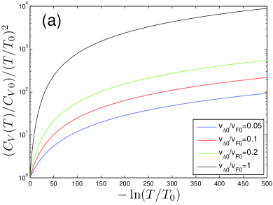
Figure 6: Numerical results for $C_{V}(T)$ obtained from the RG equation of specific heat given in [25] at different initial values $v_{\Delta 0}/v_{F0}=0.05,0.1,0.2,1$.

We notice that the specific heat obtained from equation (91) also satisfies $\lim_{T\rightarrow 0}C_{V}(T)/T^{2}\rightarrow\infty$ and $\lim_{T\rightarrow 0}\ln\left(C_{V}(T)\right)/\ln(T)\rightarrow 2$, which indicates that the specific heat is enhanced comparing to the case of non-interacting nodal fermion system. However, as will be shown in Appendix C, it cannot be expressed as a power law function. The reason is that the three parameters $C_{1}$, $C_{2}$, and $C_{3}$ appearing in equation (91) all vanish in the lowest energy limit, rather than approaching certain finite values.

Appendix C Approximate analytical expressions of DOS and specific heat

In order to show that the DOS and specific heat in clean limit do not exhibit power law behaviors, we now derive their approximate analytical expressions in the low-energy regime from the RG results. The RG equation of DOS is given by

$$\frac{d\ln\rho}{d\ln\omega}=\frac{1+C_{1}-C_{2}-C_{3}}{1-C_{1}+C_{2}}$$ (92)

in the absence of disorders. In the lowest energy limit, we know that the velocity ratio $v_{\Delta}/v_{F}\rightarrow 0$. The parameters $C_{1}$, $C_{2}$, and $C_{3}$, being functions of $v_{\Delta}/v_{F}$, all vanish [25] as $v_{\Delta}/v_{F}\rightarrow 0$. Thus the RG equation can be approximately written as

$$\frac{d\ln\rho}{d\ln\omega} \approx 1+2C_{1}-2C_{2}-C_{3}$$ (93)

$$\approx 1-\frac{2}{N}\frac{v_{\Delta}}{v_{F}}a_{1}+\frac{2}{N}\frac{v_{\Delta}}{v_{F}}a_{2}-\left(\frac{8}{\pi^{2}}\ln\left(\frac{v_{F}}{v_{\Delta}}\right)-a_{3}\right)\frac{1}{N}\frac{v_{\Delta}}{v_{F}}$$

$$\approx 1-\left(2a_{1}-2a_{2}-a_{3}\right)\frac{1}{N}\frac{v_{\Delta}}{v_{F}}-\frac{8}{N\pi^{2}}\ln\left(\frac{v_{F}}{v_{\Delta}}\right)\frac{v_{\Delta}}{v_{F}},$$

where we have used three constants $a_{1}\approx 0.426$, $a_{2}\approx 0.348$, and $a_{3}\approx 0.96$ [24]. Substituting the approximate low-energy expression of $v_{\Delta}/v_{F}$ given in equation (25) into (93), we obtain

$$\frac{d\ln\rho}{d\ln\omega} \sim 1-\left(2a_{1}-2a_{2}-a_{3}\right)\frac{1}{N}\frac{\pi^{2}N}{8}\frac{1}{l\ln(l)}-\frac{8}{N\pi^{2}}\ln\left(\frac{8}{\pi^{2}N}l\ln(l)\right)\frac{\pi^{2}N}{8}\frac{1}{l\ln(l)}$$ (94)

$$\sim 1-a_{\rho}\frac{1}{l\ln(l)}-\frac{1}{l}-\frac{\ln\ln(l)}{l\ln(l)},$$

where $a_{\rho}=\left(2a_{1}-2a_{2}-a_{3}\right)\frac{\pi^{2}}{8}+\ln\left(\frac{8}{\pi^{2}N}\right)$. For $N=2$, $a_{\rho}\approx-1.896$. Using the relationship $\omega=\omega_{0}e^{-l}$, we can solve equation (94) and then obtain the following analytical expression

$$\rho(\omega)\sim\left(\frac{\omega}{\omega_{0}}\right)\ln\left(\frac{\omega_{0}}{\omega}\right)\left(\ln\ln\left(\frac{\omega_{0}}{\omega}\right)\right)^{a_{\rho}}\exp\left[\frac{1}{2}\left(\ln\ln\ln\left(\frac{\omega_{0}}{\omega}\right)\right)^{2}\right],$$ (95)

which is applicable for small $\omega$.

The RG equation for specific heat is shown in equation (90). At low energies, it can be approximated as

$$\frac{d\ln C_{V}}{d\ln T} \sim 2+2C_{1}-C_{2}-C_{3}$$ (96)

$$\sim 2-\frac{2}{N}\frac{v_{\Delta}}{v_{F}}a_{1}+\frac{1}{N}\frac{v_{\Delta}}{v_{F}}a_{2}-\left(\frac{8}{\pi^{2}}\ln\left(\frac{v_{F}}{v_{\Delta}}\right)-a_{3}\right)\frac{1}{N}\frac{v_{\Delta}}{v_{F}}$$

$$\sim 2-a_{C}\frac{1}{l\ln(l)}-\frac{1}{l}-\frac{\ln\ln(l)}{l\ln(l)},$$

where $a_{C}=\left(2a_{1}-a_{2}-a_{3}\right)\frac{\pi^{2}}{8}+\ln\left(\frac{8}{\pi^{2}N}\right)$. At $N=2$, $a_{C}\approx-1.466$. Using the transformation $T=T_{0}e^{-l}$, we find that the specific heat at low temperature can be well approximated by the expression

$$C_{V}(T)\sim\left(\frac{T}{T_{0}}\right)^{2}\ln\left(\frac{T_{0}}{T}\right)\left(\ln\ln\left(\frac{T_{0}}{T}\right)\right)^{a_{C}}\exp\left[\frac{1}{2}\left(\ln\ln\ln\left(\frac{T_{0}}{T}\right)\right)^{2}\right].$$ (97)

By applying the same treatment, the RG equation of specific heat presented in [25], shown in equation (91), can be approximately expressed as

$$C_{V}(T)\sim\left(\frac{T}{T_{0}}\right)^{2}\ln\left(\frac{T_{0}}{T}\right)\left(\ln\ln\left(\frac{T_{0}}{T}\right)\right)^{a_{C}^{\prime}}\exp\left[\frac{1}{2}\left(\ln\ln\ln\left(\frac{T_{0}}{T}\right)\right)^{2}\right],$$ (98)

where $a_{C}^{\prime}=\left(4a_{1}-3a_{2}-a_{3}\right)\frac{\pi^{2}}{8}+\ln\left(\frac{8}{\pi^{2}N}\right)$. At $N=2$, $a_{C}^{\prime}\approx-1.273$. The above two functions do not exhibit power law dependence on temperature.

References

References

- [1] Orenstein J and Millis A J 2000 Science 288 468
- [2] Lee P A, Nagaosa N and Wen X-G 2006 Rev. Mod. Phys. 78 17
- [3] Keimer B, Kivelsoin S A, Norman M R, Uchida S and Zaanen J 2015 Nature (London) 518 179
- [4] Tsuei C C and Kirtley J R 2000 Rev. Mod. Phys. 72 969
- [5] Damascelli A, Hussian Z and Shen Z-X 2003 Rev. Mod. Phys. 75 473
- [6] Norman M R 2005 Adv. Phys. 54 715
- [7] Uemura Y J 2004 J. Phys.: Condens. Matter 16 S4515
- [8] Norman M R 2011 Science 332 196
- [9] Scalapino 2012 Rev. Mod. Phys. 84 1383
- [10] Ando Y, Segawa K, Komiya S and Lavrov A N 2002 Phys. Rev. Lett. 88 137005
- [11] Hinkov V, Haug D, Fauquéx B, Bourges P, Sidis Y, Ivanov A, Bernhard C, Lin C T and Keimer B 2008 Science 319 597
- [12] Daou R, Chang J, LeBoeuf D, Cyr-Choinière O, Laliberté F, Doiron-Leyraud N, Ramshaw B J, Liang R, Bonn D A, Hardy W N and Taillefer L 2010 Nature (London) 463 519
- [13] Lawler M J, Fujita K, Lee J, Schmidt A R, Kohsaka Y, Kim C K, Eisaki H, Uchida S, Davis J C, Sethna J P and Kim E-A 2010 Nature (London) 466 347
- [14] Fujita K, Kim C K, Lee I, Lee J, Hamidian M H, Firmo I A, Mukhopadhyay S, Eisaki H, Uchida S, Lawler M J, Kim E-A and Davis J C 2014 Science 344 612
- [15] Kivelson S A, Fradkin E and Emery V J 1998 Nature (London) 393 550
- [16] Kivelson S A, Bindloss I P, Fradkin E, Oganesyan V, Tranquada J M, Kapitulnik A and Howald C 2003 Rev. Mod. Phys. 75 1201
- [17] Vojta M 2009 Adv. Phys. 58 699
- [18] Fradkin E, Kivelson S A, Lawler M J, Eisenstein J P, Mackenzie A P 2010 Annu. Rev. Condens. Matter Phys. 1 153
- [19] Fradkin E, Kivelson S A and Tranquada J M 2015 Rev. Mod. Phys. 87, 457
- [20] Vojta M, Zhang Y and Sachdev S 2000 Phys. Rev. Lett. 85 4940
- [21] Vojta M, Zhang Y and Sachdev S 2000 Phys. Rev. B 62 6721
- [22] Vojta M, Zhang Y and Sachdev S 2000 Int. J. Mod. Phys. B 14 3719
- [23] Kim E-A, Lawler M J, Oreto P, Sachdev S, Fradkin E and Kivelson S A 2008 Phys. Rev. B 77 184514
- [24] Huh Y and Sachdev S 2008 Phys. Rev. B 78 064512
- [25] Xu C, Qi Y and Sachdev S 2008 Phys. Rev. B 78 134507
- [26] Fritz L and Sachdev S 2009 Phys. Rev. B 80 144503
- [27] Wang J, Liu G-Z and Kleinert H 2011 Phys. Rev. B 83 214503
- [28] Liu G-Z, Wang J-R and Wang J 2012 Phys. Rev. B 85 174525
- [29] Wang J-R and Liu G-Z 2013 New J. Phys. 15 063007
- [30] Wang J and Liu G-Z 2013 New J. Phys. 15 073039
- [31] She J-H, Lawler M J and Kim E-A 2015 Phys. Rev. B 92 035112
- [32] Pomeranchuk I J 1958 Sov. Phys. JETP 8 361
- [33] Yamase H and Kohno H 2000 J. Phys. Soc. Jpn. 69 332
- [34] Yamase H and Kohno H 2000 J. Phys. Soc. Jpn. 69 2151
- [35] Halboth C J and Metzner W 2000 Phys. Rev. Lett. 85 5162
- [36] Oganesyan V, Kivelson S A and Fradkin E Phys. Rev. B 2001 64 195109
- [37] Hubbard J 1963 Proc. R. Soc. A 276 238
- [38] Anderson P W 1987 Science 235 1196
- [39] Zanchi D and Schulz H J 1996 Phys. Rev. B 54 9509
- [40] Maier T, Jarrell M, Schulthess T C, Kent P R C and White J B 2005 Phys. Rev. Lett. 95 237001
- [41] Gull E, Parcollet O and Millis A J 2013 Phys. Rev. Lett. 110 216405
- [42] Huscroft C, Jarrell M, Maier Th, Moukouri S and Tahvildarzadeh A N 2001 Phys. Rev. Lett. 86 139
- [43] Macridin A, Jarrell M, Maier T, Kent P R C and D’Azevedo E 2006 Phys. Rev. Lett. 97 036401
- [44] Gull E, Ferrero M, Parcollet O, Georges A and Millis A J 2010 Phys. Rev. B 82 155101
- [45] Fang K, Fernando G W and A. N. Kocharian 2013 J. Phys.: Condens. Matter 25 205601
- [46] Fang K, Fernando G W, Balatsky A V and Kocharian A N 2015 Phys. Lett. A 379 2230
- [47] Nersesyan A A, Tsvelik A M and Wenger F 1994 Phys. Rev. Lett. 72 2628
- [48] Nersesyan A A, Tsvelik A M and Wenger F 1995 Nucl. Phys. B 438 561
- [49] Altland A, Simons B D and Zirnbauer M R 2002 Phys. Rep. 359 283
- [50] Giuliani G F and Vignale G 2005 Quantum Theory of the Electron Liquid (Chambridge: Cambridge University Press) chapter 8
- [51] Varma C M, Littlewood P B, Schmitt-Rink S, Abrahams E and Ruckenstein A E 1989 Phys. Rev. Lett. 63 1996
- [52] Gonzalez J, Guinea F and Vozmediano M A H 1996 Phys. Rev. Lett. 77 3589
- [53] Gonzalez J, Guinea F and Vozmediano M A H 1999 Phys. Rev. B 59 R2474
- [54] Kotov V N, Uchoa B, Pereira V M, Guinea F and Castro Neto A H 2012 Rev. Mod. Phys. 84 1067
- [55] Wang J-R and Liu G-Z 2014 Phys. Rev. B 89 195404
- [56] Hofmann J, Barnes E and Das Sarma S 2014 Phys. Rev. Lett. 113 105502
- [57] Chiao M, Hill R W, Lupien C, Taillefer L, Lambert P, Gagnon R and Fournier P 2000 Phys. Rev. B 62 3554
- [58] Kopnin N B and Sonin E B 2008 Phys. Rev. Lett. 100 246808
- [59] Nandkishore R, Maciejko J, Huse D A and Sondhi S L 2013 Phys. Rev. B 87 174511
- [60] Sur S and Lee S-S 2015 Phys. Rev. B 91 125136
- [61] Goswami P and Chakravarty S 2011 Phys. Rev. Lett. 107 196803
- [62] Roy B and Das Sarma S 2014 Phys. Rev. B 90 241112(R)
- [63] Shankar R 1994 Rev. Mod. Phys. 66 129
- [64] Metlitski M A, Mross D F, Sachdev S and Senthil T 2015 Phys. Rev. B 91 115111
- [65] Fitzpatrick A L, Kachru S, Kaplan J, Raghu S, Torroba G and Wang H 2015 Phys. Rev. B 92 045118
- [66] Balatsky A V, Vekhter I and Zhu J-X 2006 Rev. Mod. Phys. 78 373
- [67] Fisher R A, Gordon J E and Phillips N E 2007 in Handbook of High-Temperature superconductivity edited by Schrieffer J R and Brooks J S (Berlin: Springer) chapter 9
- [68] Revaz B, Genoud J-Y, Junod A, Neumaier K, Erb A and Walker E 1998 Phys. Rev. Lett. 80 3364
- [69] Wright D A, Emerson J P, Woodfield B F, Gordon J E, Fisher R A and Phillips N E 1999 Phys. Rev. Lett. 82 1550
- [70] Riggs S C, Vafek O, Kemper J B, Betts J B, Migliori A, Balakirev F F, Hardy W N, Liang R, Bonn D A and Boebinger G S 2011 Nat. Phys. 7 332
- [71] Allais A and Senthil T 2012 Phys. Rev. B 86 045118;
- [72] Kivelson S A and Varma C M arXiv:1208.6498v1
- [73] Wang L and Vafek O 2013 Phys. Rev. B 88 024506
- [74] Berg E, Chen C-C and Kivelson S A 2008 Phys. Rev. Lett. 100, 027003 (2008)
- [75] Shekhter A, Ramshaw B J, Liang R, Hardy W N, Bonn D A, Balakirev F F, McDondald R D, Betts J B, Riggs S C and Migliori A 2013 Nature (London) 498 75
- [76] Zaanen J 2013 Nature (London) 498 41
- [77] Valla T, Fedorov A V, Johnson P D, Wells B O, Hulbert S L, Li Q, Gu G D and Koshizuka N 1999 Science 285 2110
- [78] Titov M L, Yashenkin A G and Aristov D N 1995 Phys. Rev. B 52 10626
- [79] Khveshchenko D V and Paaske J 2001 Phys. Rev. Lett. 86 4672
- [80] Plumb N C, Reber T J, Koralek J D, Sun Z, Douglas J F, Aiura Y, Oka K, Eisaki H and Dessau D S 2010 Phys. Rev. Lett. 105 046402
- [81] Wang J and Liu G-Z 2015 Phys. Rev. B 92 184510
- [82] Metzer W, Rohe D and Andergassen 2003 Phys. Rev. Lett. 91 066402
- [83] Dell’Anna Luca and Metzner W 2006 Phys. Rev. B 73 045127
- [84] Rech J, Pépin C and Chubukov A V 2006 Phys. Rev. B 74 195126
- [85] Garst M and Chubukov A V 2010 Phys. Rev. B 81 235105
- [86] Metlitski M A and Sachdev S 2010 Phys. Rev. B 82 075127
- [87] Isobe H, Yang B-J, Chubukov A, Schmalian J and Nagaosa N 2016 Phys. Rev. Lett. 116 076803
- [88] Cho G Y and Moon E-G 2016 Sci. Rep. 6 19198
- [89] Pelissetto A P, Sachdev S and Vicari E 2008 Phys. Rev. Lett. 101, 027005
- [90] Chubukov A V 2015 Phys. Today 68 June 46
- [91] Fernandes F M, Chubukov A V and Schmalian J 2014 Nat. Phys. 10 97
- [92] Böhmer A E, Arai T, Hardy F, Hattori T, Iye T, Wolf T, Löhneysen, Ishida K and Meingast C 2015 Phys. Rev. Lett. 114 027001
- [93] Baek S-H, Efremov D V, Ok J M, Kim J S, Brink J v d and Büchner B 2015 Nat. Mater. 14 210
- [94] Chubukov A V, Fernandes R M and Schmalian J 2015 Phys. Rev. B 91 201105(R)
- [95] Yu R and Si Q 2015 Phys. Rev. Lett. 115 116401
- [96] Glasbrenner J K, Mazin I I, Jeschke H O, Hirschfeld P J, Fernandes R M and Valenti R 2015 Nat. Phys. 11 953
- [97] Wang F, Kivelson S A and Lee D-H 2015 Nat. Phys. 11 959
- [98] Jiang K, Hu J, Ding H and Wang Z 2016 Phys. Rev. B 93 115138
- [99] Lee C-H, Yin W-G and Ku W 2009 Phys. Rev. Lett. 103 267001
- [100] Shibauchi T, Carrington A and Matsuda Y 2014 Annu. Rev. Condens. Matter Phys. 5 113
- [101] Dioguardi A P, Kissikov T, Lin C H, Shirer K R, Lawson M M, Grafe H-J, Chu J-H, Fisher I R, Fernandes R M and Curro N J 2016 Phys. Rev. Lett. 116 107202
- [102] Fernandes R M and Schmalian J 2012 Supercond. Sci. Technol. 25 084005