Cluster Sampling Filters for Non-Gaussian Data Assimilation

Abstract

This paper presents a fully non-Gaussian version of the Hamiltonian Monte Carlo (HMC) sampling filter. The Gaussian prior assumption in the original HMC filter is relaxed. Specifically, a clustering step is introduced after the forecast phase of the filter, and the prior density function is estimated by fitting a Gaussian Mixture Model (GMM) to the prior ensemble. Using the data likelihood function, the posterior density is then formulated as a mixture density, and is sampled using a HMC approach (or any other scheme capable of sampling multimodal densities in high-dimensional subspaces). The main filter developed herein is named cluster HMC sampling filter ($\mathcal{C}\mathrm{\ell}\textnormal{HMC}$). A multi-chain version of the $\mathcal{C}\mathrm{\ell}\textnormal{HMC}$ filter, namely MC-$\mathcal{C}\mathrm{\ell}\textnormal{HMC}$ is also proposed to guarantee that samples are taken from the vicinities of all probability modes of the formulated posterior. The new methodologies are tested using a quasi-geostrophic (QG) model with double-gyre wind forcing and bi-harmonic friction. Numerical results demonstrate the usefulness of using GMMs to relax the Gaussian prior assumption in the HMC filtering paradigm.

Computer Science Technical Report CSTR-4/2016

Ahmed Attia, Azam Moosavi, and Adrian Sandu

“Cluster Sampling Filters for Non-Gaussian Data Assimilation”

Compute the Future!

1 Introduction

Data assimilation (DA) is a complex process that involves combining information from different sources in order to produce accurate estimates of the true state of a physical system such as the atmosphere. Sources of information include computational models of the system, a background probability distribution, and observations collected at discrete time instances. With model state denoted by $\mathbf{x}\,\in\mathbb{R}^{\textsc{n}_{\textnormal{var}}}\,,$ the prior probability density $\mathcal{P}^{\rm b}(\mathbf{x})$ encapsulates the knowledge about the system state before incorporating any other source of information such as the observations. Let $\mathbf{y}\,\in\mathbb{R}^{\textnormal{m}}$ be a measurement (observation) vector. The observation likelihood function $\mathcal{P}(\mathbf{y}|\mathbf{x})$ quantifies the mismatch between the model predictions (of observed quantities) and the collected measurements. A standard application of Bayes’ theorem provides the posterior probability distribution $\mathcal{P}(\mathbf{x}|\mathbf{y})$ that provides an improved description of the unknown true state of the system of interest.

In the ideal case where the underlying probability distributions are Gaussian, the model dynamics is linear, and the observations are linearly related to the model state, the posterior can be obtained analytically for example by applying Kalman filter (KF) equations  [26, 25]. For large dimensional problems the computational cost of the standard Kalman filter is prohibitive, and in practice the probability distributions are approximated using small ensembles. The ensemble-based approximation has led to the ensemble Kalman filter (EnKF) family of methods [9, 13, 14, 22]. Several modifications of EnKF, for example [19, 23, 40, 32, 36, 38], have been introduced in the literature to solve practical DA problems of different complexities.

One of the drawbacks of the EnKF family is the reliance on an ensemble update formula that comes from the linear Gaussian theory. Several approaches have been proposed in the literature to alleviate the limitations of the Gaussian assumptions. The maximum likelihood ensemble filter (MLEF) [27, 41, 42] computes the maximum a posteriori estimate of the state in the ensemble space. The iterative EnKF [18, 32] (IEnKF) extends MLEF to handle nonlinearity in models as well as in observations. IEnKF, however, assumes that the underlying probability distributions are Gaussian and the analysis state is best estimated by the posterior mode.

These families of filters can generally be tuned (e.g., using inflation and localization) for optimal performance on the problem at hand. However, if the posterior is a multimodal distribution, these filters are expected to diverge, or at best capture a single probability mode, especially in the case of long-term forecasts. Only a small number of filtering methodologies designed to work in the presence of highly non-Gaussian errors are available, and their efficiency with realistic models is yet to be established.

The Hybrid/Hamiltonian Monte Carlo (HMC) sampling filter was proposed in [6] as a fully non-Gaussian filtering algorithm, and has been extended to the four-dimensional (smoothing) setting in [6, 4, 5, 7]. The HMC sampling filter is a sequential DA filtering scheme that works by directly sampling the posterior probability distribution via an HMC approach [12, 39]. The HMC filter is designed to handle cases where the underlying probability distributions are non-Gaussian. Nevertheless, the first HMC formulation presented in [6] assumes that the prior distribution can always be approximated by a Gaussian distribution. This assumption was introduced for simplicity of implementation; however, it can be too restrictive in many cases, and may lead to inaccurate conclusions. This strong assumption needs to be relaxed in order to accurately sample from the true posterior, while preserving computational efficiency.

This work relaxes the Gaussian prior assumption in the original HMC formulation. Specifically, the prior is represented by a Gaussian Mixture Model (GMM) that is fitted to the forecast ensemble via a clustering step. The posterior is formulated accordingly. In the analysis step the resulting mixture posterior is sampled following a HMC approach. The analysis phase, however, can be easily modified to incorporate any other efficient direct sampling method. The resulting algorithm is named the cluster HMC ($\mathcal{C}\mathrm{\ell}\textnormal{HMC}$) sampling filter. In order to improve the sampling from the mixture posterior a more efficient version, named $\mathcal{C}\mathrm{\ell}\textnormal{HMC}$ filter (MC-$\mathcal{C}\mathrm{\ell}\textnormal{HMC}$), is also discussed.

Using a GMM to approximate the prior density, given the forecast ensemble, was presented in [2, 36] as a means to solve the nonlinear filtering problem. In [2], a continuous approximation of the prior density was built as a sum of Gaussian kernels, where the number of kernels is equal to the ensemble size. Assuming a Gaussian likelihood function, the posterior was formulated as a GMM with updated mixture parameters. The updated means and covariance matrices of the GMM posterior were obtained by applying the convolution rule of Gaussians to the prior mixture components and the likelihood, and the analysis ensemble was generated by direct sampling from the GMM posterior. On the other hand, the approach presented in [36] works by fitting a GMM to the prior ensemble with number of mixture components detected using Akaike information criterion. The EnKF equations are applied to each of the components in the mixture distribution to generate an analysis ensemble from the GMM posterior.

Unlike the existing approaches [2, 36], the methodology proposed herein is fully non-Gaussian, and does not limit the posterior density to a Gaussian mixture distribution or Gaussian likelihood functions. Here we sample the posterior distribution using a Hamiltonian Monte Carlo approach, however the direct sampling method can be replaced with any efficient analysis algorithm capable of dealing with high-dimensional multimodal distributions.

The remaining part of the paper is organized as follows. Section 2 reviews the original formulation of the HMC sampling filter. Section 3 presents the new algorithms $\mathcal{C}\mathrm{\ell}\textnormal{HMC}$ and MC-$\mathcal{C}\mathrm{\ell}\textnormal{HMC}$. Numerical results and discussions are presented in Section 4. Conclusions are drawn in Section 5.

2 The HMC Sampling Filter

In this section we present a brief overview of the HMC sampling methodology, followed by the original formulation of the HMC sampling filter.

2.1 HMC sampling

HMC sampling follows an auxiliary-variable approach [8, 37] to accelerate the sampling process of Markov chain Monte-Carlo (MCMC) algorithms. In this approach, the MCMC sampler is devoted to sampling the joint probability density of the target variable, along with an auxiliary variable. The auxiliary variable is chosen carefully to allow for the construction of a Markov chain that mixes faster, and is easier to simulate than sampling the marginal density of the target variable [20].

The main component of the HMC sampling scheme is an auxiliary Hamiltonian system that plays the role of the proposal (jumping) distribution. The Hamiltonian dynamical system operates in a phase space of points $(\mathbf{p},\mathbf{x})\in\mathbb{R}^{2\textsc{n}_{\textnormal{var}}}\,,$ where the individual variables are the position $\mathbf{x}\in\mathbb{R}^{\textsc{n}_{\textnormal{var}}}\,,$ and the momentum $\mathbf{p}\in\mathbb{R}^{\textsc{n}_{\textnormal{var}}}$. The total energy of the system, given the position and the momentum, is described by the Hamiltonian function $H(\mathbf{p},\mathbf{x})$. A general formulation of the Hamiltonian function (the Hamiltonian) of the system is given by:

$$H(\mathbf{p},\mathbf{x})=\frac{1}{2}\,\mathbf{p}^{T}\mathbf{M}^{-1}\mathbf{p}-\log(\phi(\mathbf{x}))=\frac{1}{2}\,\mathbf{p}^{T}\mathbf{M}^{-1}\mathbf{p}+\mathcal{J}(\mathbf{x})\,,$$ (1)

where $\mathbf{M}\in\mathbb{R}^{\textsc{n}_{\textnormal{var}}\times\textsc{n}_{\textnormal{var}}}$ is a symmetric positive definite matrix referred to as the mass matrix. The first term in the sum (1) quantifies the kinetic energy of the Hamiltonian system, while the second term is the associated potential energy.

The dynamics of the Hamiltonian system in time is described by the following ordinary differential equations (ODEs):

$$\frac{d\mathbf{x}}{dt}=\nabla_{\mathbf{p}}\,H\,,\qquad\frac{d\mathbf{p}}{dt}=-\nabla_{\mathbf{x}}\,H.$$ (2)

The time evolution of the system (2) in the phase space is described by the flow: [29, 33]

$$\Phi_{T}:\mathbb{R}^{2\textsc{n}_{\textnormal{var}}}\rightarrow\mathbb{R}^{2\textsc{n}_{\textnormal{var}}},\quad\Phi_{T}\bigl{(}\mathbf{p}(0),\mathbf{x}(0)\bigr{)}=\bigl{(}\mathbf{p}(T),\mathbf{x}(T)\bigr{)},$$ (3)

which maps the initial state of the system $(\mathbf{p}(0),\mathbf{x}(0))$ to $(\mathbf{p}(T),\mathbf{x}(T))\,,$ the state of the system at time $T$. In practical applications, the analytic flow $\Phi_{T}$ is replaced by a numerical solution using a time reversible and symplectic numerical integration method [34, 33]. The length of the Hamiltonian trajectory $T$ can generally be long, and may lead to instability of the time integrator if the step size is set to $T$. In order to accurately approximate $\Phi_{T}\,,$ the symplectic integrator typically takes $m$ steps of size $h=T/m$ where $h$ is chosen such as to maintain stability. We will use $\Phi_{T}$ hereafter to represent the numerical approximation of the Hamiltonian flow.

Given the formulation of the Hamiltonian (1), the dynamics of the Hamiltonian system is governed by the equations

$$\frac{d\mathbf{x}}{dt}=\mathbf{M}^{-1}\mathbf{p}\,,\qquad\frac{d\mathbf{p}}{dt}=-\nabla_{\mathbf{x}}\mathcal{J}(\mathbf{x})\,.$$ (4)

The canonical probability distribution of the state $(\mathbf{p},\mathbf{x})$ of the Hamiltonian system in the phase space $\mathbb{R}^{2\textsc{n}_{\textnormal{var}}}\,,$ upto a scaling factor, is given by

$$\exp{(-H(\mathbf{p},\mathbf{x}))}=\exp{\left(-\frac{1}{2}\mathbf{p}^{T}\mathbf{M}^{-1}\mathbf{p}-\mathcal{J}(\mathbf{x})\right)}\propto\exp{\left(-\frac{1}{2}\mathbf{p}^{T}\mathbf{M}^{-1}\mathbf{p}\right)}\,\phi(\mathbf{x}).$$ (5)

The product form of this joint probability distribution shows that the two variables $\mathbf{p},\,\text{and }\mathbf{x}$ are independent [34]. The marginal distribution of the momentum variable is Gaussian, $\mathbf{p}\sim\mathcal{N}(0,\mathbf{M})\,,$ while the marginal distribution of the position variable is proportional to the negative-logarithm (negative-log) of the potential energy, that is $\mathbf{x}\sim f(\mathbf{x})\propto\phi(\mathbf{x})=\exp{\left(-\mathcal{J}(\mathbf{x})\right)}$. Here $f(\mathbf{x})$ is the normalized marginal density of the position variable, while $\phi(\mathbf{x})$ drops the scaling factor (e.g. the normalization constant) of the density function.

In order to draw samples $\{\mathbf{x}(e)\}_{e=1,2,\ldots,\textsc{n}_{\textnormal{ens}}}$ from a given probability distribution $f(\mathbf{x})\propto\phi(\mathbf{x})\,,$ HMC makes the following analogy with the Hamiltonian mechanical system (2). The state $\mathbf{x}$ is viewed as a position variable, and an auxiliary momentum variable $\mathbf{p}\sim\mathcal{N}(0,\,\mathbf{M})$ is included. The negative-log of the target probability density $\mathcal{J}(\mathbf{x})=-\log(\phi(\mathbf{x}))$ is viewed as the potential energy of an auxiliary Hamiltonian system. The kinetic energy of the system is given by the negative-log of the Gaussian distribution of the auxiliary momentum variable. The mass matrix $\mathbf{M}$ is a user-defined parameter that is assumed to be symmetric positive definite. To achieve favorable performance of the HMC sampler, $\mathbf{M}$ is generally assumed to be diagonal, with values on the diagonal chosen to reflect the scale of the components of the target variable under the target density [6, 29]. The HMC sampler proceeds by constructing a Markov chain whose stationary distribution is set to the canonical joint density (5). The chain is initialized to some position and momentum values, and at each step of the chain, a Hamiltonian trajectory starting at the current state is constructed to propose a new state. A Metropolis-Hastings-like acceptance rule is used to either accept or reject the proposed state. Since both position and momentum are statistically independent, the retained position samples are actually sampled from the target density $f(\mathbf{x})$. The collected momentum samples are discarded, and the position samples are returned as the samples from the target probability distribution $f(\mathbf{x})$.

The performance of the HMC sampling scheme is greatly influenced by the settings of the Hamiltonian trajectory, that is the choice of the two parameters $m,\,h$. The step size $h$ should be small enough to maintain stability, while $m$ should be generally large for the sampler to reach distant points in the state space. The parameters of the Hamiltonian trajectory can be set empirically [29] to achieve an acceptable rejection rate of at most $25\%~{}30\%\,,$ or be automatically adapted using automatic tuning schemes such as the No-U-Turn sampler(NUTS) [21], or the Riemannian Manifold HMC sampler (RMHMC) [17].

The ideas presented in this work can be easily extended to incorporate any of the HMC sampling algorithms with automatically tuned parameters. In this paper we tune the parameters of the Hamiltonian trajectory following the empirical approach, and focus on the sampler performance due to the choice of the prior distribution in the sequential filtering context.

2.2 HMC sampling filter

In the filtering framework, following a perfect-model approach, the posterior distribution $\mathcal{P}^{\rm a}(\mathbf{x}_{k})$ at a time instance $t_{k}$ follows from Bayes’ theorem:

$$\mathcal{P}^{\rm a}(\mathbf{x}_{k})=\mathcal{P}(\mathbf{x}_{k}|\mathbf{y}_{k})=\frac{\mathcal{P}(\mathbf{y}_{k}|\mathbf{x}_{k})\mathcal{P}^{\rm b}(\mathbf{x}_{k})}{\mathcal{P}(\mathbf{y}_{k})}\propto\mathcal{P}(\mathbf{y}_{k}|\mathbf{x}_{k})\mathcal{P}^{\rm b}(\mathbf{x}_{k})\,,$$ (6)

where $\mathcal{P}^{\rm b}(\mathbf{x}_{k})$ is the prior distribution, $\mathcal{P}(\mathbf{y}_{k}|\mathbf{x}_{k})$ is the likelihood function, all at time instance $t_{k}$. $\mathcal{P}(\mathbf{y}_{k})$ acts as a scaling factor and is ignored in the HMC context.

As mentioned in Section 1, the formulation of the HMC sampling filter proposed in [6] assumes that the prior distribution $\mathcal{P}^{\rm b}(\mathbf{x}_{k})$ can be represented by a Gaussian distribution $\mathcal{N}(\mathbf{x}^{\textnormal{b}}_{k},\,\mathbf{\mathbf{B}_{k}})\,,$ that is

$$\mathcal{P}^{\rm b}(\mathbf{x}_{k})=\frac{(2\pi)^{-\frac{\textsc{n}_{\textnormal{var}}}{2}}}{\sqrt{|\mathbf{B}_{k}|}}\,\exp{\left(-\frac{1}{2}\lVert\mathbf{x}_{k}-\mathbf{x}^{\textnormal{b}}_{k}\rVert^{2}_{\mathbf{B}_{k}^{-1}}\right)}\,,$$ (7)

where $\mathbf{x}^{\textnormal{b}}_{k}\,,$ is the background state, and $\mathbf{B}_{k}\in\mathbb{R}^{\textsc{n}_{\textnormal{var}}\times\textsc{n}_{\textnormal{var}}}$ is the background error covariance matrix. The background state $\mathbf{x}^{\textnormal{b}}_{k}$ is generally taken as the mean of an ensemble of forecasts $\{\mathbf{x}^{\textnormal{b}}_{k}(e)\}_{e=1,\,2,\,\ldots,\,\textsc{n}_{\textnormal{ens}}}\,,$ obtained by forward model runs from a previous assimilation cycle. The associated weighted norm is defined as:

$$\mathbf{\lVert a-b\rVert^{2}_{\mathbf{C}}={(a-b)^{T}}{C}{(a-b)}}.$$ (8)

Under the traditional, yet non-restrictive assumption, that the observation errors are distributed according to a Gaussian distribution with zero mean, and observation error covariance matrix $\mathbf{R}_{k}\in\mathbb{R}^{\textnormal{m}\times\textnormal{m}}\,,$ the likelihood function takes the form

$$\mathcal{P}(\mathbf{y}_{k}|\mathbf{x}_{k})=\frac{(2\pi)^{-\frac{\textnormal{m}}{2}}}{\sqrt{|\mathbf{R}_{k}|}}\,\exp{\left(-\frac{1}{2}\lVert\mathbf{y}_{k}-\mathcal{H}_{k}(\mathbf{x}_{k})\rVert^{2}_{\mathbf{R}_{k}^{-1}}\right)}\,,$$ (9)

where $\mathcal{H}_{k}:\mathbb{R}^{\textsc{n}_{\textnormal{var}}}\to\mathbb{R}^{\textnormal{m}}$ is the observation operator that maps a given state $\mathbf{x}_{k}$ to the observation space at time instance $t_{k}$. The dimension of the observation space m is generally much smaller than the state space dimension, that is $\textnormal{m}\ll\textsc{n}_{\textnormal{var}}$.

The posterior follows immediately from (6), (7), and (9) as:

$$\mathcal{P}^{\rm a}(\mathbf{x}_{k}) \propto \phi(\mathbf{x}_{k})\,=\,\exp{\Bigl{(}-\mathcal{J}(\mathbf{x}_{k})\Bigr{)}}\,,$$ (10a)

$$\mathcal{J}(\mathbf{x}_{k}) = \frac{1}{2}\lVert\mathbf{x}_{k}-\mathbf{x}^{\textnormal{b}}_{k}\rVert^{2}_{\mathbf{B}_{k}^{-1}}+\frac{1}{2}\lVert\mathbf{y}_{k}-\mathcal{H}_{k}(\mathbf{x}_{k})\rVert^{2}_{\mathbf{R}_{k}^{-1}}\,,$$ (10b)

where $\mathcal{J}(\mathbf{x}_{k})$ is the negative-log of the posterior distribution (10a). The derivative of $\mathcal{J}(\mathbf{x}_{k})$ with respect to the system state $\mathbf{x}_{k}$ is given by

$$\nabla_{\mathbf{x}}\mathcal{J}(\mathbf{x}_{k})=\mathbf{B}^{-1}_{k}\,(\mathbf{x}_{k}-\mathbf{x}^{\textnormal{b}}_{k})-\mathbf{H}_{k}^{T}\,\mathbf{R}^{-1}_{k}\,\bigl{(}\mathbf{y}_{k}-\mathcal{H}_{k}(\mathbf{x})\bigr{)}\,,$$ (11)

where $\mathbf{H}_{k}=\mathcal{H}_{k}^{\prime}(\mathbf{x})$ is the linearized observation operator (e.g. the Jacobian).

The HMC sampling filter [6] proceeds in two steps, namely a forecast step and an analysis step. Given an analysis ensemble of states $\{\mathbf{x}^{\textnormal{a}}_{k-1}{(e)}\}_{e=1,2,\ldots,\textsc{n}_{\textnormal{ens}}}$ at time $t_{k-1}\,,$ an ensemble of forecasts at time $t_{k}$ is generated using the forward model $\mathcal{M}$:

$$\mathbf{x}^{\textnormal{b}}_{k}{(e)}=\mathcal{M}_{t_{k-1}\rightarrow t_{k}}\left(\mathbf{x}^{\textnormal{a}}_{k-1}{(e)}\right),\quad e=1,2,\ldots,\textsc{n}_{\textnormal{ens}}.$$ (12)

In the analysis step, the posterior (10) is sampled by running a HMC sampler with potential energy set to (10a), where $\mathbf{B}_{k}$ is approximated using the available ensemble of forecasts.

The formulation of the HMC filter presented in [6], and reviewed above, tends to be restrictive due to the assumption that the prior is always approximated by a Gaussian distribution. The prior distribution can be viewed as the result of propagating the posterior of the previous assimilation cycle using model dynamics. In the case of nonlinear model dynamics, the prior distribution is a nonlinear transformation of a non-Gaussian distribution which is generally expected to be non-Gaussian. Tracking the prior distribution exactly however is not possible, and a relaxation assumption must take place.

We propose conducting a more accurate density estimation of the prior, by fitting a GMM to the available prior ensemble, replacing the Gaussian prior with a Gaussian mixture prior.

3 Cluster Sampling Filters

3.1 Mixture models

The probability distribution $\mathcal{P}(\mathbf{x})$ is said to be a mixture of $\textsc{n}_{\textnormal{c}}$ probability distributions $\{\mathcal{C}_{i}(\mathbf{x})\}_{i=1,2,\ldots,\textsc{n}_{\textnormal{c}}}$, if $\mathcal{P}(\mathbf{x})$ takes the form:

$$\mathcal{P}(\mathbf{x})=\sum_{i=1}^{\textsc{n}_{\textnormal{c}}}{\tau_{i}\,\mathcal{C}_{i}(\mathbf{x})}\quad\textnormal{where}\quad\tau_{i}>0,~{}\forall i~{}~{}\textnormal{and}~{}~{}\sum_{i=1}^{\textsc{n}_{\textnormal{c}}}{\tau_{i}}=1\,.$$ (13)

The weights $\tau_{i}$ are commonly referred to as the mixing weights, and $\mathcal{C}_{i}(\mathbf{x})$ are the densities of the mixing components.

3.1.1 Gaussian mixture models (GMM)

A GMM is a special case of (13) where the mixture components are Gaussian densities, that is $\mathcal{C}_{i}(\mathbf{x})=\mathcal{N}(\mathbf{x};\Theta_{i})$ with $\Theta_{i}=\{\mu_{i},\,\mathbf{\Upsigma}_{i}\}$ being the parameters of the $i^{th}$ Gaussian component.

Fitting a GMM to a given data set is one of the most popular approaches for density estimation. Given a data set $\{\mathbf{x}(e)\}_{e=1,\,2,\,\ldots,\,\textsc{n}_{\textnormal{ens}}}\,,$ sampled from an unknown probability distribution $\mathcal{P}(\mathbf{x})$, one can estimate the density function $\mathcal{P}(\mathbf{x})$ by a GMM; the parameters of the GMM, i.e. the mixing weights $\tau_{i}$, the means $\mu_{i}$, and the covariances $\mathbf{\Upsigma}_{i}\,$ of the mixture components, can be inferred from the data.

The most popular approach to obtain the maximum likelihood estimate of the GMM parameters is the expectation-maximization (EM) algorithm [11]. EM is an iterative procedure that alternates between two steps, expectation (E) and maximization (M). At iteration $t+1$ the E-step computes the expectation of the complete log-likelihood based on the posterior probability of $\mathbf{x}$ belonging to the $i^{th}$ component, with the parameters $\Theta^{\{t\}}$ from the previous iteration. In particular, the following quantity $Q(\Uptheta|\Uptheta^{\{t\}})$ is evaluated:

$$\begin{split}Q(\Uptheta|\Uptheta^{\{t\}})&=\sum_{e=1}^{\textsc{n}_{\textnormal{ens}}}\sum_{i=1}^{\textsc{n}_{\textnormal{c}}}r_{e,i}\,\log{\big{(}\tau_{i}\,\mathcal{N}\left(\mathbf{x}(e);\Theta_{i}\right)\big{)}}\,,\\ r_{e,i}&=\frac{\tau_{i}^{\{t\}}\;\mathcal{N}\left(\mathbf{x}(e);\Theta_{i}^{\{t\}}\right)}{\sum_{\ell=1}^{\textsc{n}_{\textnormal{c}}}{\tau_{\ell}^{\{t\}}\;\mathcal{N}\left(\mathbf{x}(e);\Theta_{\ell}^{\{t\}}\right)}}\,,\\ w_{i}&=\sum_{e=1}^{\textsc{n}_{\textnormal{ens}}}r_{e,i}\,.\end{split}$$ (14)

Here $\Uptheta=\{\tau_{i},\Theta_{i}\}_{i=1\dots\textsc{n}_{\textnormal{c}}}$ is the parameter set of all the mixture components, and $r_{e,i}$ is the probability that the $e^{th}$ ensemble member lies under the $i^{th}$ mixture component.

In the M-step, the new parameters $\Uptheta^{\{t+1\}}=\arg\max_{\Uptheta}\,Q$ are obtained by maximizing the conditional probability $Q$ in (14) with respect to the parameters $\Uptheta$. The updated parameters $\Uptheta^{\{t+1\}}$ are given by the analytical formulas:

$$\tau_{i}^{\{t+1\}} =\frac{\sum_{e=1}^{\textsc{n}_{\textnormal{ens}}}{r_{e,i}}}{\textsc{n}_{\textnormal{ens}}}=\frac{w_{i}}{\textsc{n}_{\textnormal{ens}}}\,,$$ (15)

$$\mu_{i}^{\{t+1\}} =\sum_{e=1}^{\textsc{n}_{\textnormal{ens}}}{\mathbf{x}(e)\,\frac{r_{e,i}}{w_{i}}}\,,$$

$$\Upsigma_{i}^{\{t+1\}} =\sum_{e=1}^{\textsc{n}_{\textnormal{ens}}}{\left(\mathbf{x}(e)-\mu_{i}^{\{t+1\}}\right)\left(\mathbf{x}(e)-\mu_{i}^{\{t+1\}}\right)^{T}\,\frac{r_{e,i}}{w_{i}}}\,.$$

To initialize the parameters for the EM iterations, the mixing weights are simply chosen to be equal $\tau_{i}=\textsc{n}_{\textnormal{c}}^{-1}$, the means $\mu_{i}$ can be randomly selected from the given ensemble, and the covariance matrices of the components can be all set to covariance matrix of the full ensemble. Regardless of the initialization, the convergence of the EM algorithm is ensured by the fact that it monotonically increases the observed data log-likelihood at each iteration [11], that is:

$$\sum_{e=1}^{\textsc{n}_{\textnormal{ens}}}{\log{\left(\sum_{i=1}^{\textsc{n}_{\textnormal{c}}}{\tau_{i}^{\{t+1\}}\,\mathcal{N}\left(\mathbf{x}(e);\Theta_{i}^{\{t+1\}}\right)}\right)}}\geq\sum_{e=1}^{\textsc{n}_{\textnormal{ens}}}{\log{\left(\sum_{i=1}^{\textsc{n}_{\textnormal{c}}}{\tau_{i}^{\{t\}}\,\mathcal{N}\left(\mathbf{x}(e);\Theta_{i}^{\{t\}}\right)}\right)}}\,.$$

EM algorithm achieves the improvement of the data log-likelihood indirectly by improving the quantity $Q(\Uptheta|\Uptheta^{\{t\}})$ over consecutive iterations, i.e. $Q(\Uptheta|\Uptheta^{\{t+1\}})\geq Q(\Uptheta|\Uptheta^{\{t\}})$.

3.1.2 Model selection

Before EM iterations start, the number of mixture components $\textsc{n}_{\textnormal{c}}$ must be detected. To choose the number of components in the prior mixture model selection is employed. Model selection is a process of selecting a model in the set of a candidate models that gives the best trade-off between model fit and complexity. Here, the best number of components $\textsc{n}_{\textnormal{c}}$ can be selected with common model selection methodologies such as Akaike Information Criterion (AIC) and Bayesian Information Criterion (BIC):

$$AIC =-2\,\sum_{e=1}^{\textsc{n}_{\textnormal{ens}}}{\log{\left(\sum_{i=1}^{\textsc{n}_{\textnormal{c}}}{\widehat{\tau}_{i}\,\mathcal{N}\left(\mathbf{x}(e);\widehat{\Theta}_{i}\right)}\right)}}+{2\,(3\textsc{n}_{\textnormal{c}}-1)}\,,$$ (16)

$$BIC =-2\,\sum_{e=1}^{\textsc{n}_{\textnormal{ens}}}{\log{\left(\sum_{i=1}^{\textsc{n}_{\textnormal{c}}}{\widehat{\tau}_{i}\,\mathcal{N}\left(\mathbf{x}(e);\widehat{\Theta}_{i}\right)}\right)}}+{\log(\textsc{n}_{\textnormal{ens}})\,(3\textsc{n}_{\textnormal{c}}-1)}\,,$$

where $\{\widehat{\tau}_{i},\,\widehat{\Theta}_{i}\}_{i=1\dots\textsc{n}_{\textnormal{c}}}$ is the set of optimal parameters for the candidate GMM model with $\textsc{n}_{\textnormal{c}}$ components.

The best number of components $\textsc{n}_{\textnormal{c}}$ minimizes the AIC or BIC criterion [24, 35]. The main difference between the two criteria, as explained by the second terms in Equation (16), is that BIC imposes greater penalty on the number of parameters ($3\textsc{n}_{\textnormal{c}}-1$) of the candidate GMM model. For small or moderate numbers of samples BIC often chooses models that are too simple because of its heavy penalty on complexity.

3.2 Cluster HMC sampling filter ($\mathcal{C}\mathrm{\ell}\textnormal{HMC}$)

The prior distribution is approximated by a GMM fitted to the forecast ensemble, e.g., using an EM clustering step. The prior PDF reads:

$$\mathcal{P}^{\rm b}(\mathbf{x}_{k})=\sum_{i=1}^{\textsc{n}_{\textnormal{c}}}{\mathbf{\tau}_{k,i}\,\mathcal{N}(\mathbf{x};\mathbf{\mu}_{k,i},\,\mathbf{\Upsigma}_{k,i})}\,=\sum_{i=1}^{\textsc{n}_{\textnormal{c}}}{\mathbf{\tau}_{k,i}\,\frac{(2\pi)^{-\frac{\textsc{n}_{\textnormal{var}}}{2}}}{\sqrt{|\mathbf{\Upsigma}_{k,i}|}}\,\exp{\left(-\frac{1}{2}\lVert\mathbf{x}-\mathbf{\mu}_{k,i}\rVert^{2}_{\mathbf{\mathbf{\Upsigma}_{k,i}}^{-1}}\right)}}\,,$$ (17)

where the weights $\mathbf{\tau}_{k,i}$ quantify the probability that an ensemble member $\mathbf{x}_{k}(e)$ belongs to the $i^{th}$ component, and $(\mathbf{\mu}_{k,i},\,\mathbf{\Upsigma}_{k,i})$ are the mean and the covariance matrix associated with the $i^{th}$ component of the mixture model at time instance $t_{k}$.

Assuming Gaussian observation errors, the posterior can be formulated using equations (6), (9), and (17) as follows:

$$\begin{split}f(\mathbf{x}_{k})&=\mathcal{P}^{\rm a}(\mathbf{x}_{k})\\ &=\frac{(2\pi)^{-\frac{\textnormal{m}}{2}}}{\sqrt{|\mathbf{R}_{k}|}}\,\exp{\left(-\frac{1}{2}\lVert\mathcal{H}_{k}(\mathbf{x}_{k})-\mathbf{y}_{k}\rVert^{2}_{\mathbf{R}_{k}^{-1}}\right)}\,\sum_{i=1}^{\textsc{n}_{\textnormal{c}}}{\mathbf{\tau}_{k,i}\,\frac{(2\pi)^{-\frac{\textsc{n}_{\textnormal{var}}}{2}}}{\sqrt{|\mathbf{\Upsigma}_{k,i}|}}\,\exp{\left(-\frac{1}{2}\lVert\mathbf{x}_{k}-\mathbf{\mu}_{k,i}\rVert^{2}_{\mathbf{\mathbf{\Upsigma}_{k,i}}^{-1}}\right)}}\\ &\propto\phi(\mathbf{x}_{k})=\sum_{i=1}^{\textsc{n}_{\textnormal{c}}}{\frac{\mathbf{\tau}_{k,i}}{\sqrt{|\mathbf{\Upsigma}_{k,i}|}}\,\exp{\left(-\frac{1}{2}\lVert\mathbf{x}_{k}-\mathbf{\mu}_{k,i}\rVert^{2}_{\mathbf{\mathbf{\Upsigma}_{k,i}}^{-1}}-\frac{1}{2}\lVert\mathcal{H}_{k}(\mathbf{x}_{k})-\mathbf{y}_{k}\rVert^{2}_{\mathbf{R}_{k}^{-1}}\right)}}\,.\end{split}$$ (18)

In general the posterior PDF (18) will not correspond to a Gaussian mixture due to the nonlinearity of the observation operator. This makes analytical solutions not possible. Here we seek to sample directly from the posterior PDF (18).

The HMC sampling requires setting the potential energy term in the Hamiltonian (1) to the negative-log of the posterior distribution (18). The potential energy term $\mathcal{J}(\mathbf{x}_{k})$ is:

$$\mathcal{J}(\mathbf{x}_{k}) =-\log{\left(\sum_{i=1}^{\textsc{n}_{\textnormal{c}}}{\frac{\mathbf{\tau}_{k,i}}{\sqrt{|\mathbf{\Upsigma}_{k,i}|}}\,\exp{\left(-\frac{1}{2}\lVert\mathbf{x}_{k}-\mathbf{\mu}_{k,i}\rVert^{2}_{\mathbf{\mathbf{\Upsigma}_{k,i}}^{-1}}-\frac{1}{2}(\lVert\mathcal{H}_{k}(\mathbf{x}_{k})-\mathbf{y}_{k}\rVert^{2}_{\mathbf{R}_{k}^{-1}}\right)}}\right)}$$ (19a)

$$=\frac{1}{2}\lVert\mathcal{H}_{k}(\mathbf{x}_{k})-\mathbf{y}_{k}\rVert^{2}_{\mathbf{R}_{k}^{-1}}-\log{\left(\sum_{i=1}^{\textsc{n}_{\textnormal{c}}}{\frac{\mathbf{\tau}_{k,i}}{\sqrt{|\mathbf{\Upsigma}_{k,i}|}}\,\exp{\left(-\frac{1}{2}\lVert\mathbf{x}_{k}-\mathbf{\mu}_{k,i}\rVert^{2}_{\mathbf{\mathbf{\Upsigma}_{k,i}}^{-1}}\right)}}\right)}$$

$$=\frac{1}{2}\lVert\mathcal{H}_{k}(\mathbf{x}_{k})-\mathbf{y}_{k}\rVert^{2}_{\mathbf{R}_{k}^{-1}}-\log{\left(\sum_{i=1}^{\textsc{n}_{\textnormal{c}}}{\frac{\mathbf{\tau}_{k,i}}{\sqrt{|\mathbf{\Upsigma}_{k,i}|}}\,\exp{\big{(}-\mathcal{J}_{k,i}(\mathbf{x}_{k})\big{)}}}\right)}\,,$$

where

$$\mathcal{J}_{k,i}(\mathbf{x}_{k})=\frac{1}{2}\lVert\mathbf{x}_{k}-\mathbf{\mu}_{k,i}\rVert^{2}_{\mathbf{\mathbf{\Upsigma}_{k,i}}^{-1}}\,.$$ (19b)

Equation (19) is expected to suffer from numerical difficulties due to evaluating the logarithm of a sum of very small values. To address the accumulation of roundoff errors, and without loss of generality, we assume from now on that the terms in Equation (19) under the sum are sorted in decreasing order, i.e. $(\mathbf{\tau}_{k,i}/\sqrt{|\mathbf{\Upsigma}_{k,i}|})\,\exp{\left(-\mathcal{J}_{k,i}(\mathbf{x}_{k})\right)}\,>\,(\tau_{k,i+1}/\sqrt{|\mathbf{\Upsigma}_{k,i+1}|})\,\exp{\left(-\mathcal{J}_{k,i+1}(\mathbf{x}_{k})\right)}$, $\forall\,i=1,\ldots,\textsc{n}_{\textnormal{c}}-1$.

The potential energy function (19) is rewritten as:

$$\mathcal{J}(\mathbf{x}_{k}) =\frac{1}{2}\lVert\mathcal{H}_{k}(\mathbf{x}_{k})-\mathbf{y}_{k}\rVert^{2}_{\mathbf{R}_{k}^{-1}}$$ (20a)

$$\hskip 28.45274pt-\left[\log{\left(\frac{\tau_{k,1}\,\exp{\left(-\mathcal{J}_{k,1}(\mathbf{x}_{k})\right)}}{\sqrt{|\mathbf{\Upsigma}_{k,1}|}}\right)}+\log{\left(1+\sum_{i=2}^{\textsc{n}_{\textnormal{c}}}{\frac{\frac{\mathbf{\tau}_{k,i}}{\sqrt{|\mathbf{\Upsigma}_{k,i}|}}\,\exp{\left(-\mathcal{J}_{k,i}(\mathbf{x}_{k})\right)}}{\frac{\tau_{k,1}}{\sqrt{|\mathbf{\Upsigma}_{k,1}|}}\,\exp{\left(-\mathcal{J}_{k,1}(\mathbf{x}_{k})\right)}}}\right)}\right]$$

$$=\frac{1}{2}\lVert\mathcal{H}_{k}(\mathbf{x}_{k})-\mathbf{y}_{k}\rVert^{2}_{\mathbf{R}_{k}^{-1}}+\mathcal{J}_{k,1}(\mathbf{x}_{k})$$ (20b)

$$\hskip 28.45274pt-\log{\left(\frac{\tau_{k,1}}{\sqrt{|\mathbf{\Upsigma}_{k,1}|}}\right)}-\log{\left(1+\sum_{i=2}^{\textsc{n}_{\textnormal{c}}}{\frac{\mathbf{\tau}_{k,i}\,\sqrt{|{\Upsigma}_{k,1}|}}{\tau_{k,1}\,\sqrt{|\mathbf{\Upsigma}_{k,i}|}}\,\exp{\big{(}\mathcal{J}_{k,1}(\mathbf{x}_{k})-\mathcal{J}_{k,i}(\mathbf{x}_{k})\big{)}}}\right)}.$$

The gradient of the potential energy (20) is:

$$\nabla_{\mathbf{x}_{k}}\mathcal{J}(\mathbf{x}_{k}) =\mathbf{H}_{k}^{T}\mathbf{R}_{k}^{-1}(\mathcal{H}_{k}(\mathbf{x}_{k})-\mathbf{y}_{k})+\nabla_{\mathbf{x}_{k}}\mathcal{J}_{k,1}(\mathbf{x}_{k})$$ (21a)

$$\quad-\frac{1}{\left(1+\sum_{i=2}^{\textsc{n}_{\textnormal{c}}}{\frac{\tau_{k,i}\,\sqrt{|\mathbf{\Upsigma}_{k,1}|}}{\tau_{k,1}\,\sqrt{|\mathbf{\Upsigma}_{k,i}|}}\,\exp\big{(}\mathcal{J}_{k,1}(\mathbf{x}_{k})-\mathcal{J}_{k,i}(\mathbf{x}_{k})\big{)}}\right)}$$

$$\hskip 28.45274pt\cdot\sum_{i=2}^{\textsc{n}_{\textnormal{c}}}\Big{\{}\frac{\mathbf{\tau}_{k,i}\,\sqrt{|\Upsigma_{k,1}|}}{\tau_{k,1}\,\sqrt{|\mathbf{\Upsigma}_{k,i}|}}\,\exp\big{(}\mathcal{J}_{k,1}(\mathbf{x}_{k})-\mathcal{J}_{k,i}(\mathbf{x}_{k})\big{)}\cdot$$

$$\hskip 56.9055pt\cdot\Bigl{[}\nabla_{\mathbf{x}_{k}}\mathcal{J}_{k,1}(\mathbf{x}_{k})-\nabla_{\mathbf{x}_{k}}\mathcal{J}_{k,i}(\mathbf{x}_{k})\Bigr{]}\Big{\}}\,,$$

where $$\nabla_{\mathbf{x}_{k}}\mathcal{J}_{k,i}(\mathbf{x}_{k})$$ is given by:

$$\nabla_{\mathbf{x}_{k}}\mathcal{J}_{k,i}(\mathbf{x}_{k})=\mathbf{\Upsigma}_{k,i}^{-1}(\mathbf{x}_{k}-\mathbf{\mu}_{k,i})\,\,\quad\forall\,i=1,2,\ldots,\textsc{n}_{\textnormal{c}}.$$ (21b)

In the case where the mixture contains a single component (one Gaussian distribution) the potential energy function (20) and it’s gradient (21) reduce to the following, respectively:

$$\begin{split}\mathcal{J}(\mathbf{x}_{k})&=\frac{1}{2}\lVert\mathbf{x}_{k}-\mathbf{x}^{\textnormal{b}}_{k}\rVert^{2}_{\mathbf{B}_{k}^{-1}}+\frac{1}{2}\lVert\mathcal{H}_{k}(\mathbf{x}_{k})-\mathbf{y}_{k}\rVert^{2}_{\mathbf{R}_{k}^{-1}}\,,\\ \nabla_{\mathbf{x}_{k}}\mathcal{J}(\mathbf{x}_{k})&=\mathbf{B}_{k}^{-1}\left(\mathbf{x}_{k}-\mathbf{x}^{\textnormal{b}}_{k}\right)+\mathbf{H}_{k}^{T}\mathbf{R}_{k}^{-1}\left(\mathcal{H}_{k}(\mathbf{x}_{k})-\mathbf{y}_{k}\right)\,.\end{split}$$ (22)

This shows that the $\mathcal{C}\mathrm{\ell}\textnormal{HMC}$ sampling filter proposed herein reduces to the original HMC filter the EM algorithm detects a single component during the prior density approximation phase.

The $\mathcal{C}\mathrm{\ell}\textnormal{HMC}$ sampling algorithm

As in the HMC sampling filter, information about the analysis probability density at the previous time $t_{k-1}$ is captured by the analysis ensemble of states $\{\mathbf{x}^{\textnormal{a}}_{k-1}{(e)}\}_{e=1,\ldots,\textsc{n}_{\textnormal{ens}}}$. The forecast step consists of two stages. First, the model (12) is used to integrate each analysis ensemble member forward to time $t_{k}$ where observations are available. Next, a clustering scheme (e.g., EM) is used to generate the parameters of the GMM. The analysis step constructs a Markov chain starting from an initial state $\mathbf{x}_{k}^{0}$, and proceeds by sampling the posterior PDF (18) at stationarity. Here the superscript over $\mathbf{x}_{k}$ refers to the iteration number in the Markov chain.

The steps of the $\mathcal{C}\mathrm{\ell}\textnormal{HMC}$ sampling filter are detailed in Algorithm 1. As discussed in [6], Algorithm 1 can be used either as a non-Gaussian filter, or as a replenishment tool for parallel implementations of the traditional filters such as EnKF.

1:  Forecast step: given an analysis ensemble $\{\mathbf{x}^{\textnormal{a}}_{k-1}{(e)}\}_{e=1,2,\ldots,\textsc{n}_{\textnormal{ens}}}$ at time $t_{k-1}$;

1. generate the forecast ensemble using the model $\mathcal{M}$:

   $$\mathbf{x}^{\textnormal{b}}_{k}{(e)}=\mathcal{M}_{t_{k-1}\rightarrow t_{k}}\left(\mathbf{x}^{\textnormal{a}}_{k-1}{(e)}\right),\quad e=1,2,\ldots,\textsc{n}_{\textnormal{ens}}.$$

2. Use AIC/BIC criteria to detect the number of mixture components $\textsc{n}_{\textnormal{c}}$ in the GMM, then use EM to estimate the GMM parameters $\{(\mathbf{\tau}_{k,i};\,\mathbf{\mu}_{k,i},\,\mathbf{\Upsigma}_{k,i})\}_{i=1,2,\ldots,\textsc{n}_{\textnormal{c}}}$.

2:  Analysis step: given the observation $\mathbf{y}_{k}$ at time point $t_{k}\,,$ follow the steps $i$ to $v$:

1. Initialize the Markov Chain ($\mathbf{x}_{k}^{0}$) to be to the best estimate available, e.g. to the mean of the joint forecast ensemble, or the mixture component mean with maximum likelihood.

2. Choose a positive definite mass matrix $\mathbf{M}$. A recommended choice is to set $\mathbf{M}$ to be a diagonal matrix whose diagonal is equal to the diagonal of the posterior precision matrix. The precisions calculated from the prior ensemble can be used as a proxy.

3. Set the potential energy function to (20), and it’s derivative to (21).

4. Initialize the chain with a state $\mathbf{x}_{k}^{0}$ and generate $\textsc{n}_{\textnormal{ens}}$ ensemble members from the posterior distribution (18) as follows:

   1. Draw a random vector $\mathbf{p}^{r}\sim\mathcal{N}(0,\mathbf{M})$.

   2. Use a symplectic numerical integrator (e.g. Verlet, 2-Stage, or 3-Stage [34, 6]) to advance the current state $(\mathbf{p}^{r},\,\mathbf{x}_{k}^{r})$ by a pseudo-time increment $T$ to obtain a proposal state $(\mathbf{p}^{*},\,\mathbf{x}_{k}^{*})$:

      $$(\mathbf{p}^{*},\,\mathbf{x}_{k}^{*})=\Phi_{T}\bigl{(}(\mathbf{p}^{r},\,\mathbf{x}_{k}^{r})\bigr{)}.$$ (23)

   3. Evaluate the energy loss : $\Delta H=H(\mathbf{p}^{*},\,\mathbf{x}_{k}^{*})-H(\mathbf{p}^{r},\,\mathbf{x}_{k}^{r}).$

   4. Calculate the acceptance probability: $a^{(r)}=1\wedge e^{-\Delta H}.$

   5. Discard both $\mathbf{p}^{*},\,\mathbf{p}^{r}$.

   6. (Acceptance/Rejection) Draw a uniform random variable $u^{(r)}\sim\mathcal{U}(0,1)$:

      1. If $a^{(r)}>u^{(r)}$ accept the proposal as the next sample: $\mathbf{x}_{k}^{r+1}:=\mathbf{x}_{k}^{*}$;

      2. If $a^{(r)}\leq u^{(r)}$ reject the proposal and continue with the current state: $\mathbf{x}_{k}^{r+1}:=\mathbf{x}_{k}^{r}$.

   7. Repeat steps $1$ to $6$ until $\textsc{n}_{\textnormal{ens}}$ distinct samples are drawn.

5. Use the generated samples $\{\mathbf{x}^{\textnormal{a}}_{k}(e)\}_{e=1,2,\ldots,\textsc{n}_{\textnormal{ens}}}$ as an analysis ensemble. The analysis ensemble can be used to infer the posterior moments, e.g. posterior mean and posterior covariance matrix.

3:  Increase time $k:=k+1$ and repeat steps 1 and 2.

Algorithm 1 Cluster HMC sampling filter ($\mathcal{C}\mathrm{\ell}\textnormal{HMC}$)

3.3 Computational considerations

To initialize the Markov chain one seeks a state that is likely with respect to the analysis distribution. Therefore one can start with the background ensemble mean, or with the mean of the component that has the highest weight. Alternatively, one can apply a traditional EnKF step and use the mean analysis to initialize the chain.

The joint ensemble mean and covariance matrix can be evaluated using the forecast ensemble, or using the GMM parameters. Given the GMM parameters $(\mathbf{\tau}_{k,i};\,\mathbf{\mu}_{k,i},\,\mathbf{\Upsigma}_{k,i})$, the joint background mean and covariance matrix are, respectively:

$${\bf\overline{x}}^{\rm b}_{k} = \sum_{i=1}^{\textsc{n}_{\textnormal{c}}}{\mathbf{\tau}_{k,i}\,\mathbf{\mu}_{k,i}}\,,$$ (24a)

$$\mathbf{B}^{\rm ens}_{k} = \sum_{i=1}^{\textsc{n}_{\textnormal{c}}}{\mathbf{\tau}_{k,i}\,\mathbf{\Upsigma}_{k,i}}+\sum_{i=1}^{\textsc{n}_{\textnormal{c}}}{\mathbf{\tau}_{k,i}\,(\mathbf{\mu}_{k,i}-{\bf\overline{x}}^{\rm b}_{k})(\mathbf{\mu}_{k,i}-{\bf\overline{x}}^{\rm b}_{k})^{T}\,.}$$ (24b)

Both the potential energy (20) and it’s gradient (21) require evaluating the determinants of the covariance matrices associated with the mixture components. This is a computationally expensive process that is best avoided for large-scale problems. A simple remedy is to force the covariance matrices $\Upsigma_{k,i},\,\forall i=1,2,\ldots,\textsc{n}_{\textnormal{c}}$ to be diagonal while constructing the GMM.

When the Algorithm 1 is applied sequentially at some steps a single mixture component could be detected in the prior ensemble. In this case forcing a diagonal covariance structure does not help; in this case the ensemble covariance is calculated and the standard HMC sampler step is applied.

3.4 A multi-chain version of the $\mathcal{C}\mathrm{\ell}\textnormal{HMC}$ filter (MC-$\mathcal{C}\mathrm{\ell}\textnormal{HMC}$)

Given the special geometry of the posterior mixture distribution one can construct separate Markov chains for different components of the posterior. These chains can run in parallel to independently sample different regions of the analysis distribution. By running a Markov chain starting at each component of the mixture distribution we ensure that the proposed algorithm navigates all modes of the posterior, and covers all regions of high probability.

The parameters of the jumping distribution for each of the chains can be tuned locally based on the statistics of the ensemble points belonging to the corresponding component in the mixture. This approach is potentially very efficient, not only because it reduces the total running time of the sampler, but also because it favors an increase acceptance rate. The local ensemble size (sample size per chain) can be specified based on the prior weight of the corresponding component multiplied by the likelihood of the mean of that component. Every chain is initialized to the mean of the corresponding component in the prior mixture. The diagonal of the mass matrix can be set globally for all components, for example using the diagonal of the precision matrix of the forecast ensemble, or can be chosen locally based on the second-order moments estimated from the prior ensemble under the corresponding component in the prior mixture. This local choice of the mass matrix does not change the marginal density of the target variable.

4 Numerical Results

We first apply the proposed algorithms, $\mathcal{C}\mathrm{\ell}\textnormal{HMC}$ and MC-$\mathcal{C}\mathrm{\ell}\textnormal{HMC}$ to sample a simple one-dimensional mixture distribution. The proposed methodologies are then tested using a quasi-geostrophic (QG) model and compared against the original HMC sampling filter and against EnKF. We mainly use a nonlinear 1.5-layer reduced-gravity QG model with double-gyre wind forcing and bi-harmonic friction [31].

4.1 One-dimensional test problem

We start with a prior ensemble generated from a GMM with $\textsc{n}_{\textnormal{c}}=5$ and the following mixture parameters:

$$\begin{split}\{(\tau_{i};\,\mu_{i},\sigma_{i}^{2})\}_{i=1,\dots,5}=\{(0.2;\,-2.4,0.05),\,(0.1;\,-1.0,0.07),\,(0.1;\,0,0.02),\,\\ (0.3;\,1.0,0.06),\,(0.3;\,2.4,0.1)\,\}\,.\end{split}$$ (25)

The EM algorithm is used to construct a GMM approximation of the true probability distribution from which the given prior ensemble is drawn. The model selection criterion used here is AIC. The generated GMM approximation of the prior has $\textsc{n}_{\textnormal{c}}=4$ and the following parameters:

$$\begin{split}\{(\tau_{i};\,\mu_{i},\sigma_{i}^{2})\}_{i=1,\dots,4}=\{(0.169;\,-2.370,0.052),\,(0.278;\,-0.727,0.423),\\ (0.229;\,1.070,0.065),\,(0.324;\,2.436,0.159)\,\}\,.\end{split}$$ (26)

The prior ensemble and the GMM approximation of the true prior are shown in Figure 1.

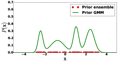
Figure 1: The one-dimensional example. A random sample of size $\textsc{n}_{\textnormal{ens}}=100$ generated from a GMM with parameters given by (25), and a GMM constructed by EM algorithm with AIC model selection criterion.

Assuming the observation likelihood function is given by:

$$\mathcal{P}(\mathbf{y}|\mathbf{x})=\frac{1}{\sqrt{1.2}\,\sqrt{2\pi}}\,\,\exp{\Bigl{(}-\frac{1}{2}\,\frac{\left(\mathbf{x}-\mathbf{y}\right)^{2}}{1.2}\Bigr{)}}\,,$$ (27)

with an observation $\mathbf{y}=-0.06858$, the posterior and the histograms of $1000$ sample points generated by $\mathcal{C}\mathrm{\ell}\textnormal{HMC}$, and MC-$\mathcal{C}\mathrm{\ell}\textnormal{HMC}$ algorithms, are shown in Figure 2. In this example, the symplectic integrator used is Verlet with pseudo-time stepping parameters $T=mh$ with $m=20$, and $h=0.05$. Since the chains are initialized to the means of the prior mixture components, the burn-in stage is waived, i.e.. the number of burn-in steps is set to zero. To reduce the correlation between the ensemble members of one chain we discard $15$ states (mixing steps) between each two consecutive sampled points. In the MC-$\mathcal{C}\mathrm{\ell}\textnormal{HMC}$ filter, the ensemble size per component (per chain) is set to $\textsc{n}_{\textnormal{ens}}\times\ell_{i}\times\tau_{i}$, where $\ell_{i}$ is the likelihood of the mean of the $i^{\rm th}$ component in the prior mixture.

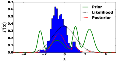
(a) $\mathcal{C}\mathrm{\ell}\textnormal{HMC}$

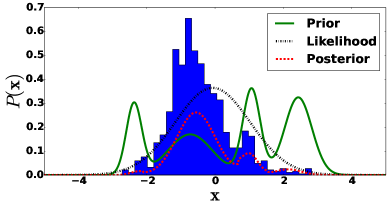
(b) MC-$\mathcal{C}\mathrm{\ell}\textnormal{HMC}$

Figure 2: The one-dimensional example. A GMM, a Gaussian likelihood, and the resulting posterior, along with histograms of $1000$ sample points generated by the $\mathcal{C}\mathrm{\ell}\textnormal{HMC}$, and the MC-$\mathcal{C}\mathrm{\ell}\textnormal{HMC}$ sampling algorithms. The sampling schemes are indicated under each panel. The symplectic integrator used is Verlet with pseudo-time stepping parameters $T=mh$ with $m=20$, and $h=0.045$. The number of burn-in steps is zero, and the number of mixing steps is $15$.

The results reported in Figures 2(a) and 2(b) show that both $\mathcal{C}\mathrm{\ell}\textnormal{HMC}$ and MC-$\mathcal{C}\mathrm{\ell}\textnormal{HMC}$ algorithms are capable of generating ensembles with mass distribution accurately representing the underlying target posterior. $\mathcal{C}\mathrm{\ell}\textnormal{HMC}$ however fails to sample one of the probability modes, while MC-$\mathcal{C}\mathrm{\ell}\textnormal{HMC}$ generates samples from the vicinities of all posterior probability modes.

An implementation of the $\mathcal{C}\mathrm{\ell}\textnormal{HMC}$ and MC-$\mathcal{C}\mathrm{\ell}\textnormal{HMC}$ sampling algorithms is available from [3].

4.2 Quasi-geostrophic model

We employ the QG-1.5 model described by Sakov and Oke [31]. This model is a numerical approximation of the equations:

$$q_{t} =\psi_{x}-\varepsilon J(\psi,q)-A\Delta^{3}\psi+2\pi\sin(2\pi y)\,,$$ (28)

$$q =\Delta\psi-F\psi\,,$$

$$J(\psi,q) \equiv\psi_{x}q_{x}-\psi_{y}q_{y}\,,$$

where $\Delta:=\partial^{2}/\partial x^{2}+\partial^{2}/\partial y^{2}$ and $\psi$ is either the stream function or the surface elevation. We use the values of the model coefficients  (28) from [31], as follows: $F=1600$, $\varepsilon=10^{-5}$, and $A=2\times 10^{-12}$. The domain of the model is a $1\times 1$ [space units] square, with $0\leq x\leq 1,\,0\leq y\leq 1\,,$ and is discretized by a grid of size $129\times 129$ (including boundaries). Boundary conditions used are $\psi=\Delta\psi=\Delta^{2}\psi=0$. The model state dimension is $\textsc{n}_{\textnormal{var}}=16641$, while the model trajectories belong to affine subspaces with dimensions of the order of $10^{2}-10^{3}$ [31].

The time integration scheme used is the fourth-order Runge-Kutta scheme with a time step $1.25$ [time units].

For all experiments in this work, the model is run over $1000$ model time steps, with observations made available every $10$ time steps. In this synthetic model the scales are not relevant, and we use generic space, time, and solution amplitude units.

4.2.1 Observations and observation operators

Two observation operators are used with this model.

• First we use a standard linear operator to observe $300$ components of $\psi$. The observation error variance is $4.0$  [units squared]. Synthetic the observations are obtained by adding white noise to measurements of the see height level (SSH) extracted from a model run with lower viscosity.

• The second observation operator measures the magnitude of the flow velocity $\sqrt{u^{2}+v^{2}}$. The flow velocity components $u,\,v$ are obtained using a finite difference approximation of the following relations to the stream function:

  $$u=+\frac{\partial\psi}{\partial y}\,,\quad v=-\frac{\partial\psi}{\partial x}.$$ (29)

In both cases, the observed components are uniformly distributed over the state vector length, with a random offset, that is updated at each assimilation cycle.

The reference initial state along with an example of the observational grid used, and the initial forecast state are shown in Figure 3.

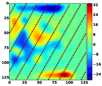
(a) Reference initial state and observational grid

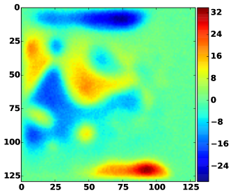
(b) Mean of the initial forecast ensemble

Figure 3: The QG-1.5 model. The red dots in panel 3(a) indicate the location of observations for one of the test cases employed.

4.2.2 Filter tuning

We used a deterministic implementation of EnKF (DEnKF) with parameters tuned as suggested in [31]. Specifically, we apply a covariance localization by means of a Hadamard product as explained in [23]. The localization function used is Gaspari-Cohn [16] with localization radius set to $12$ grid cells. Inflation is applied with factor $\delta=1.06$ to the analysis ensemble of anomalies at the end of each assimilation cycle of DEnKF.

The parameters of the HMC and $\mathcal{C}\mathrm{\ell}\textnormal{HMC}$ sampling filters are tuned empirically in a preprocessing step in the HMC filter to guarantee a rejection rate at most between $25\%$ to $30\%$. Here we tune the parameters of the Hamiltonian trajectory only once at the beginning of the assimilation experiment. Specifically, the step size parameters of the symplectic integrator are set to $h=0.075,\,m=25$ in the presence of the linear observation operator, and are set to $h=0.015,\,m=25$ when the nonlinear observation operator (29) is used. The integrator used for the Hamiltonian system in all experiments is the three-stage symplectic integrator [6, 34]. The mass matrix $\mathbf{M}$ is chosen to be a diagonal matrix whose diagonal is set to the diagonal of the precision matrix of the forecast ensemble. In the current experiments, the first $50$ steps of the Markov chains are discarded as a burn-in stage. Alternatively, one can run a suboptimal minimization of the negative-log of the posterior to achieve convergence to the posterior.

The parameters of the MC-$\mathcal{C}\mathrm{\ell}\textnormal{HMC}$ filter are set as follows. The step size parameters of the symplectic integrator are set to $h=0.05/\textsc{n}_{\textnormal{c}}$, $m=15$ in the experiments with linear observation operator, and $h=0.0075/\textsc{n}_{\textnormal{c}}$, $m=15$ in the case of the nonlinear observation operator (29). The mass matrix is a diagonal matrix whose diagonal is set to the diagonal of the precision matrix of the forecast ensemble labeled under the corresponding mixture component. To avoid numerical problems related to very small ensemble variances, for example in the case of outliers, the variances are averaged with the modeled forecast variances of $5$ [units squared].

The prior GMM is built with number of components determined using AIC model selection criteria, with a lower bound of $5$ of the number of ensemble members belonging to each component of the mixture. This lower bound is enforced as a means to ameliorate the effect of outliers on the GMM construction. In all experiments involving $\mathcal{C}\mathrm{\ell}\textnormal{HMC}$, and MC-$\mathcal{C}\mathrm{\ell}\textnormal{HMC}$, the diagonal covariances relaxation assumption is imposed. However, this structure is not imposed if only one mixture component is detected, and $\mathcal{C}\mathrm{\ell}\textnormal{HMC}$ and MC-$\mathcal{C}\mathrm{\ell}\textnormal{HMC}$ filters fall back to the original HMC filter. For cases where a component contains a very small number of ensemble members covariance tapering [15] can prove useful.

4.2.3 Assessment metrics

To assess the accuracy of the tested filters we use the root mean squared error (RMSE):

$${\rm RMSE}=\sqrt{\frac{1}{\textsc{n}_{\textnormal{var}}}\sum_{i=1}^{\textsc{n}_{\textnormal{var}}}{(x_{i}-x_{i}^{\rm true})^{2}}}\,,$$ (30)

where $\mathbf{x}^{\rm true}={\psi}^{\rm true}$ is the reference state of the system and $\mathbf{x}$ is the analysis state, e.g. the average of the analysis ensemble. Here $\textsc{n}_{\textnormal{var}}=129\times 129=16641$ is the dimension of the model state.We also use Talagrand (rank) histogram [1, 10] to assess the quality of the ensemble spread around the true state.

4.2.4 Results with linear observation operator

Figure 4 presents the RMSE (30) results of the analyses obtained using EnKF, HMC, $\mathcal{C}\mathrm{\ell}\textnormal{HMC}$, and MC-$\mathcal{C}\mathrm{\ell}\textnormal{HMC}$ filters in the presence of a linear observation operator. Figure 4 shows that the results of all HMC filter versions improve quickly at the first few assimilation windows. While the results of the original HMC filter improve quickly at the first few assimilation windows, the performance of the original HMC filter degrades compared to the DEnKF filter performance especially in the long run. We believe that the two main factors contribute to the HMC filter degradation are the parameter tuning, and the development of non-Gaussianity in the prior distribution. The $\mathcal{C}\mathrm{\ell}\textnormal{HMC}$ analysis drifts away quickly from the true trajectory. This is mainly because the HMC sampling strategy is unable to cover all probability modes in the posterior distribution. To guarantee that the sampling filter covers the truth well, the sampler has to be able to sample properly from all posterior probability modes. This is achieved by design by the MC-$\mathcal{C}\mathrm{\ell}\textnormal{HMC}$ filter. The MC-$\mathcal{C}\mathrm{\ell}\textnormal{HMC}$ version produces RMSE results comparable to the RMSE obtained by DEnKF.

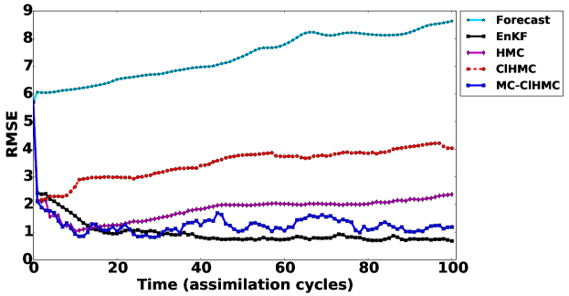
Figure 4: Data assimilation results with the linear observation operator. RMSE of the (30) analyses obtained by EnKF, HMC, $\mathcal{C}\mathrm{\ell}\textnormal{HMC}$, and MC-$\mathcal{C}\mathrm{\ell}\textnormal{HMC}$ filters.

As discussed in [6] the performance of HMC filter can be further enhanced by automatically tuning the parameters of the symplectic integrator at the beginning of each assimilation cycle. Here however we are mainly interested in assessing the performance of the new methodologies compared to the original HMC filter using equivalent settings.

It is important to note that the MC-$\mathcal{C}\mathrm{\ell}\textnormal{HMC}$ filter requires shorter Hamiltonian trajectories to explore the space under each local mixture component, which results in computational savings. Additional savings can be obtains by running the chains in parallel to sample different regions of the posterior.

Since we are not interested in only a single best estimate of the true state of the system, RMSE alone is not sufficient to judge the quality of the filtering system. The analysis ensemble sampled from the posterior should be spread widely enough to cover the truth and avoid filter collapse. The rank histograms of the analysis ensembles are shown in Figure 5. The two small spikes in Figure 5(b) suggest that the performance of the original HMC filter could be enhanced by increasing the length of the Hamiltonian trajectories in some assimilation cycles.

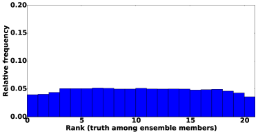
(a) DEnKF

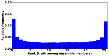
(b) HMC

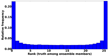
(c) $\mathcal{C}\mathrm{\ell}\textnormal{HMC}$ +AIC

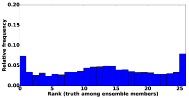
(d) MC-$\mathcal{C}\mathrm{\ell}\textnormal{HMC}$ +AIC

Figure 5: Data assimilation results with the linear observation operator. The rank histograms of where the truth ranks among posterior ensemble members. The ranks are evaluated for every $16^{th}$ variable in the state vector (past the correlation bound) at $100$ assimilation times.

The rank histogram shown in Figure 5(c) shows that the analysis ensembles produced by the $\mathcal{C}\mathrm{\ell}\textnormal{HMC}$ filter tend to be under-dispersed. Since the ensemble size is relatively small and the prior GMM is multimodal, with regions of low-probability between the different mixture components, a multimodal mixture posterior with isolated components is obtained. As explained in [30], this is a case where HMC sampling in general can suffer from being entrapped in a local minimum (and fails to jump between different high probability modes). This behavior is expected to result in ensemble collapse, as seen in Figure 5(c), leading to filter degradation in the long run as illustrated by the RMS errors shown in Figure 4.

The results shown in Figure 5(c) suggest that the analysis ensemble collected by $\mathcal{C}\mathrm{\ell}\textnormal{HMC}$ fails to cover all mixture components, thereby losing its dispersion when it is applied repetitively. This is supported by the results in Figure 6, where the rank histograms are plotted using results from the first two, five, and ten cycles, respectively.

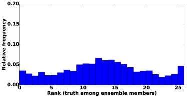
(a) $\mathcal{C}\mathrm{\ell}\textnormal{HMC}$ +AIC; first two observation windows

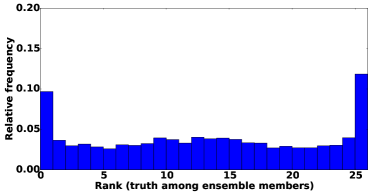
(b) $\mathcal{C}\mathrm{\ell}\textnormal{HMC}$ +AIC; first five observation windows

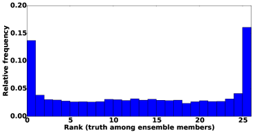
(c) $\mathcal{C}\mathrm{\ell}\textnormal{HMC}$ +AIC; first ten observation windows

Figure 6: Data assimilation results using a linear observation operator. Rank histograms of where the truth ranks among posterior ensemble members. The ranks are evaluated for every $16^{th}$ variable in the state vector (past the correlation bound). Rank histograms of $\mathcal{C}\mathrm{\ell}\textnormal{HMC}$ results obtained at the first two, five, and ten assimilation cycles respectively are shown. The model selection criterion used is AIC.

The ensemble collapse can be avoided if we force the sampler to collect ensemble members from all the probability modes. This is illustrated by the rank histograms of results obtained using the MC-$\mathcal{C}\mathrm{\ell}\textnormal{HMC}$ filter with AIC criteria as shown in Figure 5(d).

We believe that having isolated regions of high probability, e.g., with very small number of ensemble members in each component, can be the critical factor leading the poor long-term performance of $\mathcal{C}\mathrm{\ell}\textnormal{HMC}$. This is alleviated here by imposing a minimum number of $3$ ensemble points in each component, e.g. via hard assignment, of the mixture while constructing the GMM approximation of the prior.

With automatic tuning of the Hamiltonian parameters the performance of both HMC and MC-$\mathcal{C}\mathrm{\ell}\textnormal{HMC}$ filters is expected to be greatly enhanced. We have only shown the results of $\mathcal{C}\mathrm{\ell}\textnormal{HMC}$, and MC-$\mathcal{C}\mathrm{\ell}\textnormal{HMC}$ with AIC information criterion; experiments carried out using other model selection criteria such as BIC have proven to be very similar.

To help decide whether to apply the original formulation of the HMC filter, or the proposed methodology, one can run tests of non-Gaussianity on the forecast ensemble. To asses non-Gaussianity of the forecast several numeric or visualization normality tests are available, e.g., the Mardia test [28] based on multivariate extensions of skewness and kurtosis measures. Indication of non-Gaussianity can be found by visually inspecting several bivariate contour plots of the joint distribution of selected components in the state vector. Visualization methods for multivariate normality assessment such as chi-square QQ-plots can be very useful as well. Figure 7 shows several chi-square QQ-plots of the forecast ensembles generated from the result of EnKF, HMC, and MC-$\mathcal{C}\mathrm{\ell}\textnormal{HMC}$ filters at different time instances. These plots show strong signs of non-Gaussianity in the forecast ensemble, and suggest that the Gaussian-prior assumption may in general lead to inaccurate conclusions.

(a) EnKF; t=300

(b) EnKF; t=775

(c) EnKF; t=1000

(d) EnKF; t=1200

(e) HMC; t=300

(f) HMC; t=775

(g) HMC; t=1000

(h) HMC; t=1200

(i) MC-$\mathcal{C}\mathrm{\ell}\textnormal{HMC}$; t=300

(j) MC-$\mathcal{C}\mathrm{\ell}\textnormal{HMC}$; t=775

(k) MC-$\mathcal{C}\mathrm{\ell}\textnormal{HMC}$; t=1000

(l) MC-$\mathcal{C}\mathrm{\ell}\textnormal{HMC}$; t=1200

Figure 7: Data assimilation with a linear observation operator. Chi-square Q-Q plots for the forecast ensembles obtained from propagating analyses of EnKF, HMC, and MC-$\mathcal{C}\mathrm{\ell}\textnormal{HMC}$ filtering systems to times t=300, 775, 1000, and 1200 provide a strong indication of non-Gaussianity. The filtering methodology, and the assimilation time are given under each panel. Localization is applied to the ensemble covariance matrix to avoid singularity while evaluating the Mahalanobis distances of the ensemble members.

4.2.5 Results with nonlinear wind-magnitude observations

In the presence of a nonlinear observation operator the distribution is expected to show even stronger signs of non-Gaussianity. With stronger non-Gaussianity, the cluster methodology is expected to outperform the original formulation of the HMC sampling filter.

Figure 8 shows RMSE results, with the nonlinear observation operator (29), for the analyses obtained by HMC, $\mathcal{C}\mathrm{\ell}\textnormal{HMC}$, MC-$\mathcal{C}\mathrm{\ell}\textnormal{HMC}$ filtering systems. While EnKF diverges under the current settings after the third cycle (results omitted for clarity), HMC, $\mathcal{C}\mathrm{\ell}\textnormal{HMC}$, and MC-$\mathcal{C}\mathrm{\ell}\textnormal{HMC}$ continue to behave similar to the case where the linear observation operator is used.

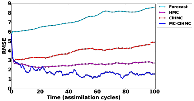
Figure 8: Data assimilation results with the nonlinear observation operator (29). RMSE of the analyses obtained by HMC, $\mathcal{C}\mathrm{\ell}\textnormal{HMC}$, and MC-$\mathcal{C}\mathrm{\ell}\textnormal{HMC}$ filtering schemes. In this experiment, EnKF analysis diverged after the third cycle, and it’s RMSE results have been omitted for clarity.

Figure 9 shows rank histograms of HMC, $\mathcal{C}\mathrm{\ell}\textnormal{HMC}$, and MC-$\mathcal{C}\mathrm{\ell}\textnormal{HMC}$, with a nonlinear observation operator. We can see that $\mathcal{C}\mathrm{\ell}\textnormal{HMC}$ performance is similar to the case when the linear observation operator is used. It seems to be entrapped into a local minimum losing its dispersion quickly. The results of the MC-$\mathcal{C}\mathrm{\ell}\textnormal{HMC}$ filter avoid this effect and show a reasonable spread.

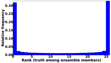
(a) HMC

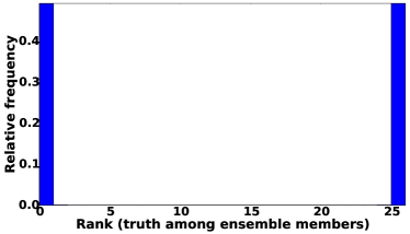
(b) $\mathcal{C}\mathrm{\ell}\textnormal{HMC}$ +AIC

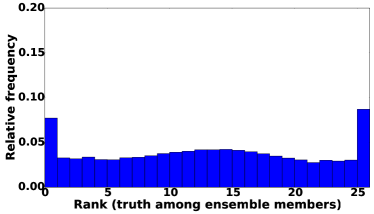
(c) MC-$\mathcal{C}\mathrm{\ell}\textnormal{HMC}$ +AIC

Figure 9: Data assimilation results using the nonlinear observation operator (29). The rank histograms of where the truth ranks among posterior ensemble members. The ranks are evaluated for every $16^{th}$ variable in the state vector (past the correlation bound) at $100$ assimilation times. The filtering scheme used is indicated under each panel.

The results presented here suggest that the cluster formulation of the HMC sampling filter is advantageous, especially in the presence of highly nonlinear observation operator, or strong indication of non-Gaussianity.

5 Conclusions and Future Work

This work presents a new formulation of the HMC sampling filter for non-Gaussian data assimilation. The new formulation, named the Cluster HMC sampling filter ($\mathcal{C}\mathrm{\ell}\textnormal{HMC}$), relaxes the Gaussian prior assumption. The prior density is represented more accurately via a GMM fitted to the forecast ensemble. The initial formulation of the $\mathcal{C}\mathrm{\ell}\textnormal{HMC}$ filter presented here is not expected to outperform the original HMC filter unless the sampler is capable of efficiently sampling multimodal distributions with modes separated by large regions of low probability. A multi-chain version of $\mathcal{C}\mathrm{\ell}\textnormal{HMC}$, namely MC-$\mathcal{C}\mathrm{\ell}\textnormal{HMC}$, is developed in order to achieve this goal.

Numerical experiments are carried out using a nonlinear 1.5-layer reduced-gravity quasi geostrophic model in the presence of observation operators of different levels of nonlinearity. The results show that the new methodologies are much more efficient that the original HMC sampling filter especially in the presence of a highly nonlinear observation operator.

The MC-$\mathcal{C}\mathrm{\ell}\textnormal{HMC}$ is an algorithm that deserves further investigation. For example the local sample sizes here are selected based on the prior weight multiplied by the likelihood of the corresponding component mean. An optimal selection of the local ensemble size is required to guarantee efficient sampling from the target distribution.

Instead of using MC-$\mathcal{C}\mathrm{\ell}\textnormal{HMC}$ filter, one can use $\mathcal{C}\mathrm{\ell}\textnormal{HMC}$ with geometrically tempered Hamiltonian sampler as recently proposed in [30], such as to guarantee navigation between separate modes of the posterior. Alternatively, the posterior distribution can be split into $\textsc{n}_{\textnormal{c}}$ target distributions with different potential energy functions and associated gradients. This is equivalent to running independent HMC sampling filters in different regions of the state space under the target posterior.

The authors have started to investigate the ideas discussed here, in addition to testing the proposed methodologies with automatically tuned HMC samplers.

References

References

- [1] Jeffrey L Anderson. A method for producing and evaluating probabilistic forecasts from ensemble model integrations. Journal of Climate, 9(7):1518–1530, 1996.
- [2] Jeffrey L Anderson and Stephen L Anderson. A Monte Carlo implementation of the nonlinear filtering problem to produce ensemble assimilations and forecasts. Monthly Weather Review, 127(12):2741–2758, 1999.
- [3] Ahmed Attia. Cluster HMC sampling algorithms: one-dimensional examples. http://csl.cs.vt.edu/software.php, 2016. [Online; accessed ].
- [4] Ahmed Attia, Vishwas Rao, and Adrian Sandu. A sampling approach for four dimensional data assimilation. In Dynamic Data-Driven Environmental Systems Science, pages 215–226. Springer, 2015.
- [5] Ahmed Attia, Vishwas Rao, and Adrian Sandu. A Hybrid Monte-Carlo sampling smoother for four dimensional data assimilation. International Journal for Numerical Methods in Fluids, 2016. fld.4259.
- [6] Ahmed Attia and Adrian Sandu. A Hybrid Monte Carlo sampling filter for non-Gaussian data assimilation. AIMS Geosciences, 1(geosci-01-00041):41–78, 2015.
- [7] Ahmed Attia, Razvan Stefanescu, and Adrian Sandu. The reduced-order Hybrid Monte-Carlo sampling smoother. International Journal for Numerical Methods in Fluids, 2016. fld.4255.
- [8] Julian Besag and Peter J Green. Spatial statistics and Bayesian computation. Journal of the Royal Statistical Society. Series B (Methodological), pages 25–37, 1993.
- [9] Gerrit Burgers, Peter Jan van Leeuwen, and Geir Evensen. Analysis scheme in the Ensemble Kalman Filter. Monthly Weather Review, 126:1719–1724, 1998.
- [10] G Candille and O Talagrand. Evaluation of probabilistic prediction systems for a scalar variable. Quarterly Journal of the Royal Meteorological Society, 131(609):2131–2150, 2005.
- [11] Arthur P Dempster, Nan M Laird, and Donald B Rubin. Maximum likelihood from incomplete data via the em algorithm. Journal of the royal statistical society. Series B (methodological), pages 1–38, 1977.
- [12] Simon Duane, Anthony D Kennedy, Brian J Pendleton, and Duncan Roweth. Hybrid Monte Carlo. Physics Letters B, 195(2):216–222, 1987.
- [13] Geir Evensen. Sequential data assimilation with a nonlinear quasi-geostrophic model using Monte Carlo methods to forcast error statistics . Journal of Geophysical Research, 99(C5):10143–10162, 1994.
- [14] Geir Evensen. The Ensemble Kalman Filter: theoretical formulation and practical implementation. Ocean Dynamics, 53, 2003.
- [15] Reinhard Furrer, Marc G Genton, and Douglas Nychka. Covariance tapering for interpolation of large spatial datasets. Journal of Computational and Graphical Statistics, 15(3), 2006.
- [16] Gregory Gaspari and Stephen E Cohn. Construction of correlation functions in two and three dimensions. Quarterly Journal of the Royal Meteorological Society, 125:723–757, 1999.
- [17] Mark Girolami and Ben Calderhead. Riemann manifold Langevin and Hamiltonian Monte Carlo methods. Journal of the Royal Statistical Society: Series B (Statistical Methodology), 73(2):123–214, 2011.
- [18] Yaqing Gu, Dean S Oliver, et al. An iterative ensemble Kalman filter for multiphase fluid flow data assimilation. Spe Journal, 12(04):438–446, 2007.
- [19] Thomas M Hamill, Jeffrey S Whitaker, and Chris Snyder. Distance-dependent filtering of background error covariance estimates in an ensemble Kalman filter. Monthly Weather Review, 129:2776–2790, 2001.
- [20] David M Higdon. Auxiliary variable methods for Markov chain Monte Carlo with applications. Journal of the American Statistical Association, 93(442):585–595, 1998.
- [21] Matthew D Hoffman and Andrew Gelman. The no-u-turn sampler: Adaptively setting path lengths in Hamiltonian Monte Carlo. The Journal of Machine Learning Research, 15(1):1593–1623, 2014.
- [22] Peter L Houtekamer and Herschel L Mitchell. Data assimilation using an ensemble Kalman filter technique . Monthly Weather Review, 126:796–811, 1998.
- [23] Peter L Houtekamer and Herschel L Mitchell. A sequential ensemble Kalman filter for atmospheric data assimilation . Monthly Weather Review, 129:123–137, 2001.
- [24] Xuelei Hu and Lei Xu. Investigation on several model selection criteria for determining the number of cluster. Neural Information Processing-Letters and Reviews, 4(1):1–10, 2004.
- [25] Rudolph E Kalman and Richard S Bucy. New results in linear filtering and prediction theory. Journal of basic engineering, 83(1):95–108, 1961.
- [26] Rudolph Emil Kalman. A new approach to linear filtering and prediction problems . Transaction of the ASME- Journal of Basic Engineering, 82:35–45, 1960.
- [27] Andrew C Lorenc. Analysis methods for numerical weather prediction. Quarterly Journal of the Royal Meteorological Society, 112:1177–1194, 1986.
- [28] Kanti V Mardia. Measures of multivariate skewness and kurtosis with applications. Biometrika, 57(3):519–530, 1970.
- [29] Radford M Neal et al. MCMC using Hamiltonian dynamics. Handbook of Markov chain Monte Carlo, 2011.
- [30] Akihiko Nishimura and David Dunson. Geometrically Tempered Hamiltonian Monte Carlo. arXiv preprint arXiv:1604.00872, 2016.
- [31] Pavel Sakov and Peter R Oke. A deterministic formulation of the ensemble Kalman filter: an alternative to ensemble square root filters. Tellus A, 60(2):361–371, 2008.
- [32] Pavel Sakov, Dean S Oliver, and Laurent Bertino. An iterative EnKF for strongly nonlinear systems. Monthly Weather Review, 140(6):1988–2004, 2012.
- [33] Jesus-Maria Sanz-Serna and Mari-Paz Calvo. Numerical Hamiltonian problems, volume 7. Chapman & Hall London, 1994.
- [34] JM Sanz-Serna. Markov chain Monte Carlo and numerical differential equations. In Current Challenges in Stability Issues for Numerical Differential Equations, pages 39–88. Springer, 2014.
- [35] Gideon Schwarz et al. Estimating the dimension of a model. The annals of statistics, 6(2):461–464, 1978.
- [36] Keston W Smith. Cluster ensemble Kalman filter. Tellus A, 59(5):749–757, 2007.
- [37] A Sokal. Monte Carlo methods in statistical mechanics: foundations and new algorithms. Springer, 1997.
- [38] Michael K Tippett, Jeffrey L Anderson, Craig H Bishop, Thomas M Hamill, and Jeffrey S Whitaker. Ensemble square root filters. Monthly Weather Review, 131:1485–1490, 2003.
- [39] Raiul Toral and AL Ferreira. A general class of Hybrid Monte Carlo methods. In Proceedings of Physics Computing, volume 94, pages 265–268, 1994.
- [40] Jeffrey S Whitaker and Thomas M Hamill. Ensemble data assimilation without perturbed observations. Monthly Weather Review, 130:1913–1924, 2002.
- [41] Milija Zupanski. Maximum likelihood ensemble filter: Theoretical aspects. Monthly Weather Review, 133(6):1710–1726, 2005.
- [42] Milija Zupanski, I Michael Navon, and Dusanka Zupanski. The Maximum Likelihood Ensemble Filter as a non-differentiable minimization algorithm. Quarterly Journal of the Royal Meteorological Society, 134(633):1039–1050, 2008.