Indirect Maximum Entropy Bandwidth

Abstract

This paper proposes a new method of bandwidth selection in kernel estimation of density and distribution functions motivated by the connection between maximisation of the entropy of probability integral transforms and maximum likelihood in classical parametric models. The proposed estimators are designed to indirectly maximise the entropy of the leave-one-out kernel estimates of a distribution function, which are the analogues of the parametric probability integral transforms.

The estimators based on minimisation of the Cramér-von Mises discrepancy, near-solution of the moment-based estimating equations, and inversion of the Neyman smooth test statistic are discussed and their performance compared in a simulation study. The bandwidth minimising the Anderson-Darling statistic is found to perform reliably for a variety of distribution shapes and can be recommended in practice.

The results will also be of interest to anyone analysing the cross-validation bandwidths based on leave-one-out estimates or evaluation of nonparametric density forecasts.

Keywords: Kernel density estimation; distribution function; probability integral transform; cross-validation; permutohedron.

AMS subject classification: 62G05, 62G07.

1 Introduction

Let $X_{1},\ldots,X_{n}$ be a sample of independent, identically distributed random variables with an absolutely continuous distribution function (d.f.) $F$ and density $f$. The kernel estimators of $F$ (KDFE) and $f$ (KDE) at a point $x$ are

$$\widehat{F}(x;b)=n^{-1}\sum_{i=1}^{n}K_{b}(x-X_{i}),\quad b\geq 0,$$ (1)

(Nadaraya, 1964; Watson and Leadbetter, 1964) and

$$\hat{f}(x;b)=n^{-1}\sum_{i=1}^{n}k_{b}(x-X_{i}),\quad b>0,$$ (2)

(Rosenblatt, 1956; Parzen, 1962) respectively, where $k_{b}(z)=k(z/b)/b$ and $K_{b}(z)=K(z/b)=\int_{-\infty}^{z/b}k(v)dv$ are the kernels, with $k$ being symmetric about the origin and integrating to unity, and $b=b_{n}$ is the bandwidth sequence. The empirical distribution function (EDF) can be obtained as a special case of (1) with $b=0$, viz. $F_{n}(x)=\widehat{F}(x;0)=n^{-1}\sum_{i=1}^{n}\mathbbm{1}\left\{X_{i}\leq x\right\}$. It is well known that under mild conditions $\widehat{F}$ and $\hat{f}$ are uniformly strongly consistent and asymptotically normal estimators of $F$ and $f$, respectively (Yamato, 1973; Silverman, 1978).

By far the most common measure of fit in kernel smoothing is the mean integrated squared error (MISE). Other less commonly applied criteria include the $L_{1}$ norm (Devroye and Györfi, 1985), the Kullback-Leibler (KL) divergence (Hall, 1987), and the Hellinger distance (Kanazawa, 1993). One consequence of using the curve-fitting framework to evaluate the quality of the estimates (1) and (2) is that in general the bandwidths optimal for KDE and KDFE differ (intuitively, the d.f. is easier to estimate than the density). For example, the bandwidths optimal in the MISE sense for $\widehat{F}$ and $\hat{f}$ are asymptotically of order $n^{-1/5}$ and $n^{-1/3}$, respectively (see e.g. Wand and Jones, 1995). Thus the ability to recover an estimate of a d.f. from that of a density, and vice versa, using the identity $\widehat{F}(x;b)=\int_{-\infty}^{x}\hat{f}(z;b)dz$ is lost.

This paper posits an alternative framework for bandwidth selection in kernel estimation of density and distribution functions. To motivate the proposed methods consider the classical parametric setup where $Z_{i}$, $i=1,\ldots,n$, are independent random variables with common d.f. $G$ and density $g$, and the model is given by the family of d.f.’s $\mathscr{F}=\{F_{\theta}(z):\theta\in\Theta\subseteq\mathbbm{R}^{p}\}$ with densities $f_{\theta}$. The model $\mathscr{F}$ may or may not contain the true distribution $G$. The probability integral transform (PIT) of $Z_{i}$ under the model $F_{\theta}$ is defined as $V_{i}(\theta)=F_{\theta}(Z_{i})$. The vector of PITs, $V(\theta)=\left(V_{1}(\theta),\ldots,V_{n}(\theta)\right)^{\mathsf{T}}$, is distributed on $I^{n}=[0,1]^{n}$, the $n$-dimensional unit hypercube placed in the positive orthant of $\mathbbm{R}^{n}$ with one vertex at the origin; the components of $V(\theta)$ are independent and have a common d.f., $Q_{\theta}(u)$, $u\in[0,1]$, say, with density $q_{\theta}$.

It is well known that under appropriate regularity conditions the following equalities hold:

$$\operatorname*{argmin}_{\theta\in\Theta}\;D\left(g\|f_{\theta}\right)=\operatorname*{argmax}_{\theta\in\Theta}\;\operatorname{E}_{G}\left[\ln f_{\theta}(Z)\right]=\operatorname*{argmax}_{\theta\in\Theta}\;h\left(U(\theta)\right)=\operatorname*{argmin}_{\theta\in\Theta}\;D\left(q_{\theta}\|r\right),$$ (3)

where $r$ denotes the uniform density on $[0,1]$, $D(g\|f)=\int g(z)\ln\left(\left.g(z)\right/f(z)\right)dz$ is the relative entropy of $g$ with respect to $f$ (the KL between $g$ and $f$), and $h(Z)=-\int f(z)\ln f(z)dz$ is the Shannon differential entropy of a random vector $Z$ with density $f$, hereinafter simply the entropy. The first two equalities underpin the quasi- (or pseudo-) maximum likelihood (Akaike, 1973; White, 1982) and the maximum spacings estimators (Shao and Hahn, 1994). The third equality in (3) can be used to motivate testing the goodness of fit or evaluation of density forecasts by checking the uniformity of PITs (Gneiting et al., 2007; Diebold et al., 1998), although such tests are usually motivated by the fact that PITs are uniform if $F_{\theta}=G$ (Neyman, 1937; Rosenblatt, 1952), thus bypassing the maximum entropy interpretation.

It is thus natural to consider an alternative class of estimators for $\theta$ defined as minimisers of KL or other distance or discrepancy measure between $Q_{\theta}$ ($q_{\theta}$) and the uniform d.f. (density). In view of (3) such estimators can be called the indirect maximum entropy (iMaxEnt) estimators. The idea of fine-tuning the model to achieve uniformity of PITs (combined with independence of $V_{i}$’s in a time series context) has been put forward in e.g. Dawid (1984), but to the best of my knowledge no such estimators have been formally studied before. Clearly, if $G=F_{\theta_{0}}\in\mathscr{F}$, then in all cases in (3) the optimum is achieved with $f_{\theta}=g$ and $V_{i}(\theta)$ independent, uniformly distributed on a unit interval. Under the appropriate regularity conditions the iMaxEnt estimators will then also be consistent for $\theta_{0}$. When $G\notin\mathscr{F}$ the pseudo-true values of iMaxEnt estimators will generally differ from the maximiser of the entropy of $V(\theta)$. However, if the model provides a close approximation to the true distribution, one can expect all such pseudo-true values to be similar.

While the iMaxEnt estimators for parametric models are not further pursued here, the ideas carry over to kernel estimation of density and distribution functions. Specifically, for a fixed kernel the estimators (1) and (2) can be viewed as a model indexed by the bandwidth parameter, and the natural analogue of the PIT under this model is the leave-one-out kernel estimate of a d.f. at a sample value $x_{i}$. Then a bandwidth which results in the joint distribution of the leave-one-out estimates being close to uniform over their support can be seen as the bandwidth indirectly maximising the Shannon entropy of PITs.

The properties of the leave-one-out estimates are examined in Section 2, and several estimation procedures for the indirect maximum entropy bandwidth are proposed. Performance of selected estimators is evaluated in a small simulation study reported in Section 3. Section 4 concludes. Proofs and other technical results are given in the appendices and the supplement.

Notation.  For a nonzero vector $w\in\mathbbm{R}^{n}$ and a real number $t$, $H_{w,t}$ denotes the hyperplane $H_{w,t}=\{x\in\mathbbm{R}^{n}:\left\langle w,x\right\rangle=t\}$. For a point $x=(x_{1},\ldots,x_{n})$ in $\mathbbm{R}^{n}$ the permutohedron $P_{n}(x)$ is the convex hull of all vectors obtained from $x$ by permutations of the coordinates, $P_{n}(x)=\mathop{\mathrm{conv}}\left((x_{\sigma(1)},\ldots,x_{\sigma(n)})|\sigma\in S_{n}\right)$, where $S_{n}$ is the symmetric group. $P_{n}(n-1,n-2,\ldots,0)$ is called the regular permutohedron. The dimension of $P_{n}(x)$ is at most $n-1$, and if not all the coordinates of $x$ are equal, then $\dim P_{n}(x)=n-1$. $\mathop{\mathrm{Vol}}\nolimits_{n-1}\left(P_{n}\right)$ denotes the usual $(n-1)$-dimensional volume of the projection of $P_{n}$ onto $x_{n}=0$.

2 Main results

2.1 Assumptions

Assumption 1

(a) $X_{1},\ldots,X_{n}$ are independent, identically distributed random variables from an absolutely continuous distribution $F$ with a bounded density function $f$;
(b) $f$ possesses a fourth derivative which is continuous and square integrable.

Assumption 2

(a) The kernel, $k:\mathbbm{R}\mapsto[0,\infty)$ is a bounded function, $k(-x)=k(x)$, $\int_{-\infty}^{\infty}k(x)dx=1$, and $\mu_{2}(k)=\int_{-\infty}^{\infty}x^{2}k(x)dx<\infty$;
(b) $\mu_{4}(k)=\int_{-\infty}^{\infty}x^{4}k(x)dx<\infty$, and $\psi_{2,1}(K)=2\int_{-\infty}^{\infty}xK(x)k(x)dx<\infty$.

Assumption 3

The bandwidth $b>0$ is a non-stochastic sequence such that as $n\to\infty$, $b\to 0$ and $bn\to\infty$.

Assumptions 1(a), 2(a), and 3 are standard in the smoothing literature. The requirement that $bn\to\infty$ in Assumption (3) is needed for consistency of the KDE (2). Assumption 2(a) is the definition of a second order kernel. Kernels of orders higher than two are not considered here because they necessarily take negative values and thus the resultant density estimates are not necessarily non-negative and the d.f. estimates not necessarily non-decreasing. This would both undermine the connection with parametric models and cause some of the subsequent results to break down.

Assumptions 1(b) and 2(b) are used for the asymptotic expansions.

2.2 The leave-one-out estimates

Considering the KDFE (1) (and KDE (2)) as a family of models indexed by a parameter $b>0$ for a given $k$, the natural analogue of the probability integral transform is the leave-one-out estimate of $F$ at $x_{i}$, $i=1,\ldots,n$, viz.

$$V_{i}(b)=\widehat{F}_{(-i)}(X_{i};b)=\frac{1}{n-1}\sum_{\begin{subarray}{c}j=1\\ j\neq i\end{subarray}}^{n}K_{b}(X_{i}-X_{j}),\qquad n\geq 2.$$ (4)

Equivalently, $V_{i}(b)=\int_{-\infty}^{x_{i}}\hat{f}_{(-i)}(z;b)dz$, where $\hat{f}_{(-i)}(z;b)$ is the KDE (2) constructed using all but the $i^{th}$ observation. Under Assumptions 1(a) and 2(a), the components of $V(b)=\left(V_{1}(b),\ldots,V_{n}(b)\right)^{\mathsf{T}}$ are identically distributed on the $[0,1]$ interval with a marginal CDF $G(v)=G(v;n,b)$, say, but are dependent by construction, viz. for $i\neq j$, $\operatorname{corr}(V_{i},V_{j})=-1/(n-1)$ by symmetry.

Lemma 1

If Assumptions 1(a) and 2(a) hold, then the support of the leave-one-out estimates $V(b)$, $b\geq 0$, is the the regular permutohedron scaled by $(n-1)^{-1}$, viz.

$$\Pi_{n}=P_{n}\left(1,(n-2)/(n-1),(n-3)/(n-1),\ldots,1/(n-1),0\right). \square$$

$\Pi_{n}$ is an $(n-1)$-dimensional polytope that lies in the central section of a unit hypercube, $\Pi_{n}\subset\left(I^{n}\cap H_{\boldsymbol{\iota}_{n},n/2}\right)$, and its barycentre is $c=\boldsymbol{\iota}_{n}/2$, where $\boldsymbol{\iota}_{n}$ is an $n$-vector of ones. In particular, $\sum_{i=1}^{n}V_{i}=n/2$ and the joint distribution of $V(b)$ is singular. $\operatorname{E}V_{j}=1/2$ and all the higher moments of $V_{j}$ approach the respective moments of the uniform distribution on $[0,1]$ as $n\to\infty$ and $b\to 0$ at the rate $\max(b^{2},n^{-1})$.

Lemma 2

If Assumptions 1(a,b), 2(a,b), and 3 hold, then as $n\to\infty$, for $r\geq 2$, $j=1,\ldots,n$,

$$\operatorname{E}V_{j}^{r}=\frac{1}{r+1}-\frac{1}{2}\mu_{2}(k)\xi_{2,r}(F)b^{2}+\frac{r-1}{2(r+1)}n^{-1}-\psi_{2,1}(K)\xi_{1,r}(F)bn^{-1}+\mathit{O}\left(\max(b^{2}n^{-1},b^{4},n^{-2})\right),$$

where for $r\geq 2$, $\xi_{2,r}(F)=\frac{r(r-1)}{2}\int_{-\infty}^{\infty}F^{r-2}(x)f^{3}(x)dx$, $\xi_{1,r}(F)=\int_{-\infty}^{\infty}\frac{r(r-1)}{2}F^{r-2}(x)f^{2}(x)dx$, and $0<\xi_{r}(F)\leq\frac{r}{2}\sup_{x}f^{2}(x)$, $0<\xi_{1,r}(F)\leq\frac{r}{2}\sup_{x}f(x)$. $\square$

2.3 The indirect maximum entropy bandwidth

Following the ideas outlined in the introduction it is natural to seek a bandwidth which maximises the entropy of $V(b)$. By the Maximum Entropy Principle, the (possibly infeasible) MaxEnt bandwidth, $b^{\circ}$, would be such that $V(b^{\circ})$ is uniformly distributed over its support, $\Pi_{n}$. Since the components of $V(b)$ are identically distributed, the marginal distribution of $V_{i}(b)$, $G(v)$, and the density, $g(v)$, are estimable. The MaxEnt bandwidth can therefore be estimated indirectly by minimising an appropriate distance or discrepancy measure between $G$ (or $g$) and the marginal d.f. (density) of the components of a random vector distributed uniformly over $\Pi_{n}$.

Lemma 3

Suppose an $n$-vector $(u_{1},\ldots,u_{n})^{\mathsf{T}}$ has a (singular) uniform distribution on a permutohedron $\Pi_{n}$, then the marginal distributions of $u_{i}$, $i=1,\ldots,n$, are identical with probability density function given by

$$l_{n}(u)=\frac{n-1}{n^{n-2}}\mathop{\mathrm{Vol}}\nolimits_{n-2}\left(P_{n-1}\left(n-1,n-2,\ldots,j+1,\;2j-1-(n-1)u,\;j-2,\ldots,0\right)\right),$$ (5)

for $u\in\left[\frac{j-1}{n-1},\frac{j}{n-1}\right]$, $j=1,\ldots,n-1$. The marginal density at $0$ and $1$ is $l_{n}(0)=l_{n}(1)=\left(1-1/n\right)^{n-2}$. $\square$

The density (5), the corresponding d.f. $L_{n}(u)=\int_{0}^{u}l_{n}(t)dt$, $u\in[0,1]$, moments or other quantities of interest can be computed exactly or approximated as described in Appendix A. Figure 1 shows the exact density $l_{n}(u)$ for $n=2,\ldots,11$ (panel A) and the approximated density for $n=100,\ldots,1000000$ (panel B). The values of the first five even central moments of a random variable with density $l_{n}(u)$ for $n$ between $2$ and $1,000,000$ are tabulated in the Supplement.

(A) Exact density (5) for $n=2,\ldots,11$	(B) Estimated density for $n=100,\ldots,1,000,000$

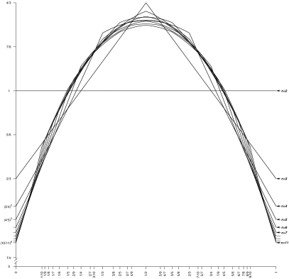
Legend: $u$ on the horizontal axes, density on the vertical axes.
Panel (B): Beta kernel density estimates (Chen, 1999) on an equispaced grid of $1000$ points from $5e8/n$ random uniform draws on $\Pi_{n}$ and bandwidth $0.001$. Estimates are symmetrised, adjusted at the endpoints, and rescaled to integrate to unity.

Figure 1: The marginal density $l_{n}(u)$

The indirect maximum entropy (iMaxEnt) bandwidth can be defined as the bandwidth which results in the distribution of $V_{i}$’s being close to the uniform distribution over $\Pi_{n}$, (5). To illustrate the idea, let $n=3$ and $f$ and $k$ be the standard normal densities. The top panel of Figure 2 shows $5,000$ random draws of $V(b)=\left(V_{1}(b),V_{2}(b),V_{3}(b)\right)^{\mathsf{T}}$ with $b=0.5,\,1.25$, and $2$. The corresponding marginal density of $V_{i}(b)$ (histogram) together with $l_{3}$ (solid line) is shown in the bottom panel. The distribution of $V(b)$ with $b=1.25$ is visually uniform over $\Pi_{3}$ with the marginal being close to $l_{3}$, whereas the left and right panels correspond to bandwidths which are too small and too big, respectively.

$5,000$ random draws
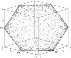
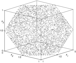
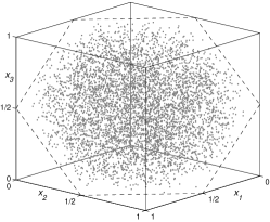
$b=0.5$	$b=1.25$	$b=2$
Marginal distribution ($1,5$ million draws)
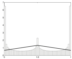
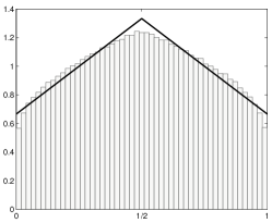
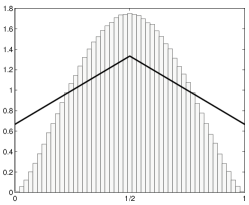
$b=0.5$	$b=1.25$	$b=2$

Figure 2: An illustration of the indirect maximum entropy bandwidth

To operationalise the definition of the iMaxEnt bandwidth the remainder of this section considers three criteria of closeness chosen chiefly for their simplicity including simple calculating forms. Small sample performance is evaluated in a simulation study reported in Section 3.

2.3.1 Minimum Cramér-von Mises estimators

Let $F$ and $G$ be two distribution functions with common support. The weighted Cramér–von Mises (CvM) discrepancy (Smirnov, 1937) is defined as

$$\omega_{\psi}^{2}(G,F)=\int_{-\infty}^{\infty}\left[G(z)-F(z)\right]^{2}\psi\left(F(z)\right)dF(z)=\int_{0}^{1}\left[G\left(F^{-1}(t)\right)-t\right]^{2}\psi(t)dt,$$ (6)

where $\psi$ is a weight function which is typically taken to be non-negative and smooth. Special cases of (6) include the classical CvM criterion, $\omega^{2}$, when $\psi(t)=1$, $t\in[0,1]$, and the Anderson-Darling (AD) statistic, $\omega_{AD}^{2}$, when $\psi(t)=t^{-1}(1-t)^{-1}$, $t\in(0,1)$ (Anderson and Darling, 1952).

The min-CvM iMaxEnt bandwidth is defined as

$$\hat{b}_{CvM}=\operatorname*{argmin}_{b>0}\;\omega_{\psi}^{2}(G_{n},L_{n}),$$ (7)

where $G_{n}=G_{n}(v;b)$ is the EDF of $V_{i}(b)$, $i=1,\ldots,n$. The CvM criterion $\omega^{2}_{\alpha;\epsilon}=\omega_{\psi}^{2}$ with the weight function $\psi(t)=t^{\alpha-1}(1-t)^{\alpha-1}\mathbbm{1}\left\{\epsilon\leq t\leq 1-\epsilon\right\}$, where $\alpha\geq 0$, and $0\leq\epsilon\ll 1/2$ is a (small) trimming constant, is attractive as it has a simple calculating form given in Appendix D and includes both $\omega^{2}=\omega^{2}_{1;0}$ and $\omega_{AD}^{2}=\omega^{2}_{0;0}$ as special cases. In practice, $L_{n}$ can be estimated on a grid of points in $[0,1]$ as described in Appendix A, and evaluation of $u_{i}=L_{n}\left(V_{i}(b)\right)$ can be done by interpolation (linear or otherwise). Then $\omega_{\alpha;\epsilon}^{2}(G_{n},L_{n})$ can be easily calculated from the order statistics $u_{(1)}\leq\cdots\leq u_{(n)}$.

An interesting connection exists between the above procedure and the Sarda (1993) cross-validation criterion (Appendix B). In particular, the unweighted version of the cross-validation criterion is numerically equivalent, up to an additive constant, to the CvM discrepancy between $G_{n}$ and the uniform d.f. on $[0,1]$, $R$, viz. $\operatorname{CV}_{1}(b)=\omega^{2}(G_{n},R)+1/(6n^{2})$. However, while asymptotically the minimiser of $\omega^{2}(G,R)$ is well defined, the integrated variance of $G_{n}$, $\operatorname{IVar}G_{n}$, adds an extra term making $\operatorname{E}\operatorname{CV}_{1}$ an increasing function of $b$. That is to say, the $\operatorname{CV}_{1}$ criterion cannot work.

The $\mathit{O}\left(bn^{-1}\right)$ term from $\operatorname{IVar}G_{n}$ causing $CV_{1}$ to break down is still present in the expansion of $\operatorname{E}\omega^{2}(G_{n},L_{n})$, of course, but it does not dominate asymptotically as in $\operatorname{E}CV_{1}$. In particular, if Conjecture 1(b) in Section 2.4 holds, then by the same method as in the proof of Lemma B.1, the leading terms in an expansion of $\omega^{2}(G,L)$ are $a_{1}b^{4}-a_{2}b^{2}n^{-1/2}+a_{3}n^{-1}$, where $a_{1}=\mu_{2}^{2}(k)\zeta_{1}(F)/4$, as in Lemma B.1, and $a_{2},a_{3}$ are some positive constants depending on $\gamma_{m}$’s in Conjecture 1(b). Thus $\operatorname{E}\omega^{2}(G_{n},L_{n})$ generally has a well-defined minimum away from zero, and the minimiser is of order $n^{-1/4}$ asymptotically. However, in finite samples, there is typically a second (local or global) minimum at $b=0$, even for the normal density. In some particularly unfavourable cases, for example for the strongly skewed distribution (#3 in Figure 5), only $\omega^{2}_{\alpha;\epsilon}$ with $\alpha$ very close to zero appears to perform well provided care is taken to ensure the correct minimum is chosen; see Figure 3 for an illustration.

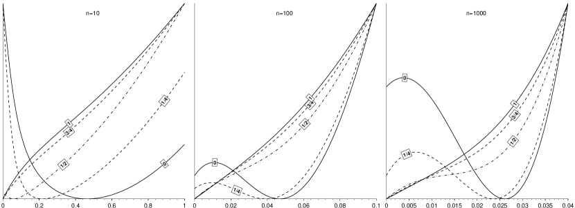
Horizontal axes–bandwidth; vertical axes (not to scale)–CvM criteria, $\omega^{2}_{\alpha;\epsilon}$, for $\alpha=0,1/4,1/2,3/4$, and $1$, and $\epsilon=0.001$.

Figure 3: CvM criteria for the strongly skewed density

2.3.2 Moment-based estimating equations

Moment-based estimators provide a simple, appealing alternative alleviating some of the problems with the min-CvM procedure. Let $m_{j,n}$, $j=2,3,\ldots$ be the central moments of the distribution $l_{n}(u)$ defined in (5). The $r$-moment iMaxEnt bandwidth, $\hat{b}_{MEE}$, can be defined as the near-solution to the $(r-1)$ estimating equations

$$n^{-1}\sum_{i=1}^{n}(V_{i}(\hat{b})-1/2)^{j}-m_{j,n}=0,\quad j=2,3,\ldots,r.$$ (8)

(Since $V_{i}$’s sum to $n/2$ for all $b$, the first moment contains no identifying information.) $\hat{b}$ in (8) can be estimated using Generalised Empirical Likelihood (GEL) methods (Newey and Smith, 2004).

The simplest moment-based bandwidth sets the sample variance of $V_{i}$’s equal to $m_{2,n}$. For example when $f$ and $k$ are both standard normal densities,

$$\operatorname{Var}V_{1}(b)=\frac{n-2}{n-1}\frac{1}{\pi}\arctan\sqrt{\frac{3+b^{2}}{1+b^{2}}}+\frac{1}{n-1}\frac{1}{\pi}\arctan\sqrt{\frac{4+b^{2}}{b^{2}}}-\frac{1}{4}.$$

The bandwidth $b$ solving $\operatorname{Var}V_{1}(b)=m_{2,n}$ is shown in Figure 4 (iMaxEnt–$m_{2}$). Bandwidths minimising the exact MISE of $\hat{f}$ (min-MISE KDE) and $\widehat{F}$ (min-MISE KDFE) are shown for comparison.

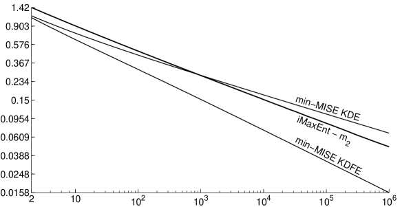
Horizontal axis–$n$, log scale; vertical axis–bandwidth, $b$, log scale.

Figure 4: $2^{nd}$ moment-based iMaxEnt bandwidth

When the true density is close to normal the $2^{nd}$ moment-based iMaxEnt bandwidth can be expected to perform well in the sense of the resultant distribution of $V_{i}$ being close to $l_{n}$ in other metrics as well. This is confirmed by the simulation study (Figure 6 in Section 3). In general, inclusion of the $3^{rd}$ and $4^{th}$ moments is advisable to capture skewness and kurtosis, respectively. However, estimators based on much higher moments are likely to become increasingly sensitive to outliers.

2.3.3 Neyman smooth test

A useful alternative to the moment-based estimators can be obtained by inverting the Neyman (1937) smooth test statistic. Let $\rho_{k}(v)$, $k=0,1,2,\ldots$ be the orthonormal shifted Legendre polynomials, i.e. orthonormal polynomials with respect to the uniform density on $[0,1]$. The Neyman smooth test statistic based on the first $r$ polynomials is defined as

$$S_{r}(b)=\sum_{j=1}^{r}\left[\frac{1}{\sqrt{n}}\sum_{i=1}^{n}\rho_{j}\left(u_{i}(b)\right)\right]^{2}=n\bar{\rho}_{r}^{\mathsf{T}}\bar{\rho}_{r},$$ (9)

where $\bar{\rho}_{r}=n^{-1}\sum_{i=1}^{n}\left(\rho_{1}(u_{i}(b)),\ldots,\rho_{r}(u_{i}(b))\right)^{\mathsf{T}}$ and $u_{i}(b)=L_{n}(V_{i}(b))$ as before. The estimator of the iMaxEnt bandwidth based on the first $r\geq 2$ polynomials is defined as a minimiser of (9), viz. $\hat{b}_{NS}=\operatorname*{argmin}_{b>0}S_{r}(b)$.

Quite generally, $\hat{b}_{MEE}$ and $\hat{b}_{NS}$ with the same $r$ can be expected to be similar as, loosely speaking, $\hat{b}_{NS}$ can be viewed as a restricted version of $\hat{b}_{MEE}$. $\hat{b}_{NS}$ is computationally faster and can be more stable with high $r$ since it does not involve computation of the covariance matrix of MEE (8). The choice of $r$ can be based on the same considerations as above; see also discussion in Bera and Ghosh (2002) and references therein.

2.4 Remarks on asymptotic behaviour

To obtain asymptotic expansions for the proposed bandwidth estimator the knowledge of the limiting behaviour of $l_{n}(u)$ in required. While there is no formal proof, intuition and simulation evidence (see Supplement) suggest that the following conjecture is true.

Conjecture 1

As $n\to\infty$

1. $l_{n}(u)$ approaches the uniform density, $l_{n}(u)\to 1$ for all $u\in(0,1)$, except at the end points where $l_{n}(0)=l_{n}(1)=\left(1-1/n\right)^{n-2}\to e^{-1}$, and

2. the moments of a random variable with density $l_{n}(u)$ approach the moments of the uniform distribution at a rate $n^{-1/2}$ from below, i.e. $\int_{0}^{1}u^{m}l_{n}(u)du=\frac{1}{m+1}-\gamma_{m}n^{-1/2}+\mathit{o}\left(n^{-1/2}\right)$ for $m\geq 2$ and some finite constants $\gamma_{m}>0$. $\square$

If Assumptions 1(a,b), 2(a,b), and 3 hold, and Conjecture 1(b) is true, then in view of Lemma 2, the bandwidth setting $G=L_{n}$ will be of order $n^{-1/4}$ as $n\to\infty$. Asymptotically, the iMaxEnt bandwidth will be in-between the KDE and KDFE MISE-minimising bandwidths, which are of order $n^{-1/5}$ and $n^{-1/3}$, respectively. This is true at least for the simple examples such as shown in Figure 4.

3 Simulation study

This section investigates performance of selected iMaxEnt bandwidth estimators in small and medium samples via simulation using the first six normal mixture distributions defined in Table 1 of Marron and Wand (1992) as examples (Figure 5). The densities have been scaled to have zero mean and unit variance. Among the advantages of working with normal mixtures is the availability of exact MISE expressions for the class of Gaussian-based kernels given in Marron and Wand (1992) for KDE and Oryshchenko (2016) for KDFE. The values of the exact MISE-minimising bandwidths for KDE and KDFE are shown in Figure 7 (‘D’ and ‘C’ bandwidths, respectively) and drawn in Figure 6 as vertical dashed and solid lines, respectively. These provide reference points for the iMaxEnt bandwidth, expected to be in-between the two asymptotically.

#1: Gaussian	#2: Skewed unimodal	#3: Strongly skewed
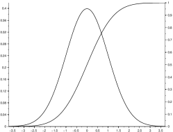
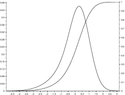
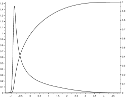
#4: Kurtotic unimodal	#5: Outlier	#6: Bimodal
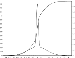
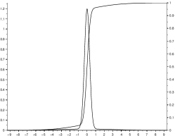
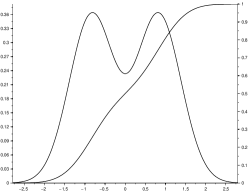
Density on the left vertical axes, d.f. on the right.

Figure 5: Selected normal mixture distributions

For each mixture distribution, Figure 6 shows density estimates and boxplots (minimum, $1^{st}$, $2^{nd}$, and $3^{rd}$ quartiles, and maximum) of the nine iMaxEnt bandwidth estimators:

• The min-CvM estimators with weight function $\psi(t)=t^{\alpha-1}(1-t)^{\alpha-1}\mathbbm{1}\left\{\epsilon\leq t\leq 1-\epsilon\right\}$ for $\alpha=0,\,1/2$, and $1/4$ (CvM-0 or AD, CvM-1/2, and CvM-1/4, respectively), and $\epsilon=0.001$.

• The MEE estimators based on the $2^{nd}$ (CUE-2), $2^{nd}$ and $3^{rd}$ (CUE-3), and $2^{nd}$, $3^{rd}$, and $4^{th}$ moments (CUE-4). These are the continuously updating estimators (CUE), which is a special case of GEL. Performance of other members of the GEL class of estimators, including Empirical Likelihood, was much worse and is therefore not shown.

• The minimum Neyman smooth test estimators based on the first 2, 3, and 4 polynomials (NSm-2, -3, and -4, respectively).

Figure 7 shows the $l_{n}$ density (thick solid line) and estimated densities of $V_{i}(b)$ for five selected values of the bandwidth: the KDE and KDFE min-MISE bandwidths (‘D’ and ‘C’) and the median values of CvM-0 (AD), NSm-2, and NSm-4 iMaxEnt bandwidths. In both Figure 6 and 7 the kernel is Gaussian, and the sample sizes are (left to right) 10, 100, and 1000. Results are based on 10 and 100 thousand replications, respectively.

As expected, all bandwidth estimators produce similar results for the normal density. This is also largely true for the moderately skewed density, although the importance of the third moment is noticeable. Somewhat surprisingly, the estimators produce not too dissimilar results for the outlier density in moderate samples, with the importance of the fourth moment now being pronounced, and the larger right tail in small samples reflecting the presence of outliers.

The situation is strikingly different for the densities with significant departures from normality. As was noted in Section 2.3.1 (Figure 3), the min-CvM bandwidth for the strongly skewed density is likely to be zero for $\alpha$ much larger than zero, which is indeed the case. The NSm-3, NSm-4, and CUE-4, but not CUE-3, yield similar results, followed by the min-AD bandwidth; all delivering the distribution of $V_{i}$ reasonably close to $l_{n}$ (Figure 7). The NSm-2 and CUE-2 behave differently, of course, since they only use the information in the second moment. The difference in behaviour of NSm-3 and CUE-3 is somewhat puzzling. Similar picture emerges for the bimodal density (#6) with the estimators using the first four moments producing the most promising results, followed closely by AD.

None of the moment-based (or Neyman smooth test) bandwidth estimators can be recommended for the kurtotic unimodal density (#4): the NSm-4 and CUE-4 estimators deliver a bandwidth which is too small, whereas the estimates using the $2^{nd}$ and $3^{rd}$ moments are too big. The min-CvM bandwidths appear to be the best in this case.

In general, the min-CvM bandwidth with $\alpha=0$ (min-AD) can be recommended for densities that exhibit significant departures from normality, although it is advisable to examine the profile of the criterion over the relevant range of $b$ to ensure the correct minimum is selected. For regularly shaped densities, the moment-based estimators may be preferred. An estimate of the resultant density or d.f. of $V_{i}$ can be used as a further diagnostic tool to ascertain the adequacy of the chosen bandwidth by either a visual examination or comparison of the distances from $l_{n}$ or $L_{n}$.

#1: Gaussian

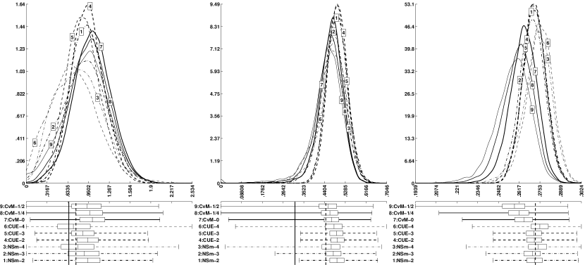
#2: Skewed unimodal

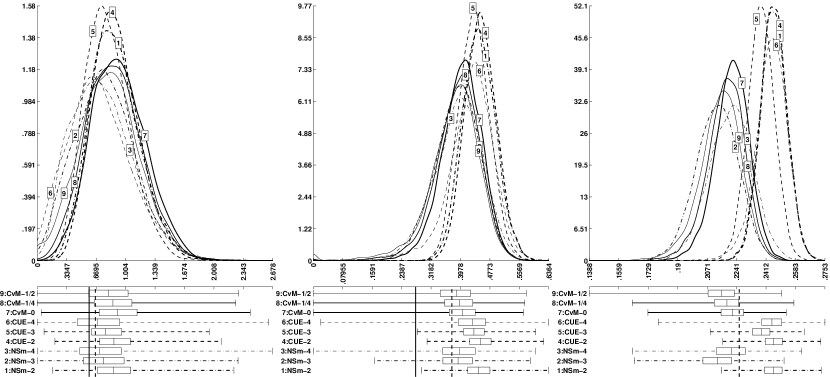
#3: Strongly skewed

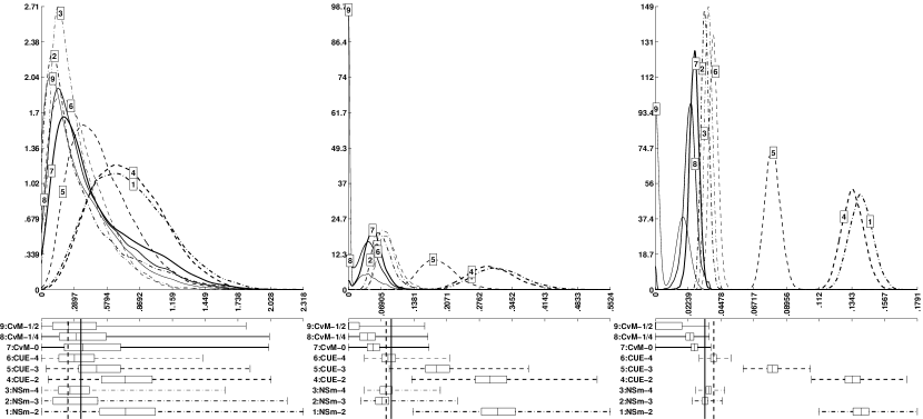
Figure 6: Performance of selected iMaxEnt bandwidth estimators

#4: Kurtotic unimodal

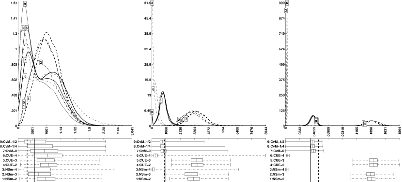
#5: Outlier

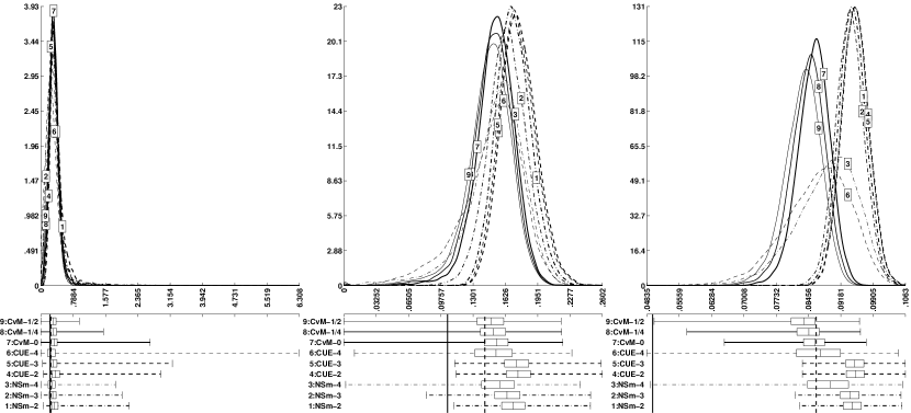
#6: Bimodal

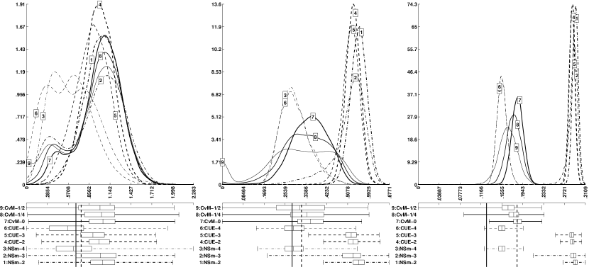
Figure 6 (Cont.): Performance of selected iMaxEnt bandwidth estimators

#1: Gaussian
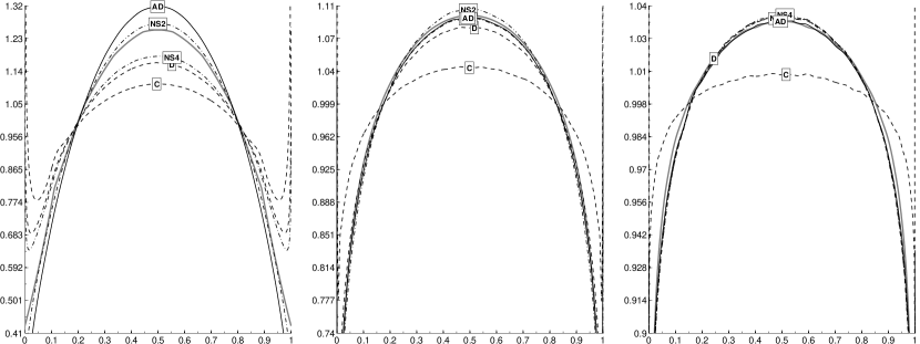
Bandwidths: NS2: 0.9374 C: 0.6495 NS4: 0.7915 D: 0.7585 AD:  1.0091	Bandwidths: NS2: 0.4931 C: 0.3147 NS4: 0.4687 D: 0.4455 AD:  0.4712	Bandwidths: NS2: 0.2717 C: 0.1517 NS4: 0.2740 D: 0.2723 AD:  0.2648
#2: Skewed unimodal
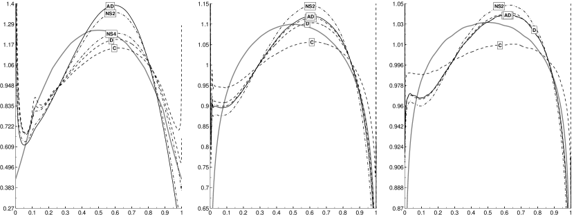
Bandwidths: NS2: 0.8636 C: 0.5896 NS4: 0.7095 D: 0.6602 AD:  0.9145	Bandwidths: NS2: 0.4465 C: 0.2764 NS4: 0.3955 D: 0.3743 AD:  0.4034	Bandwidths: NS2: 0.2454 C: 0.1317 NS4: 0.2211 D: 0.2257 AD:  0.2218
#3: Strongly skewed
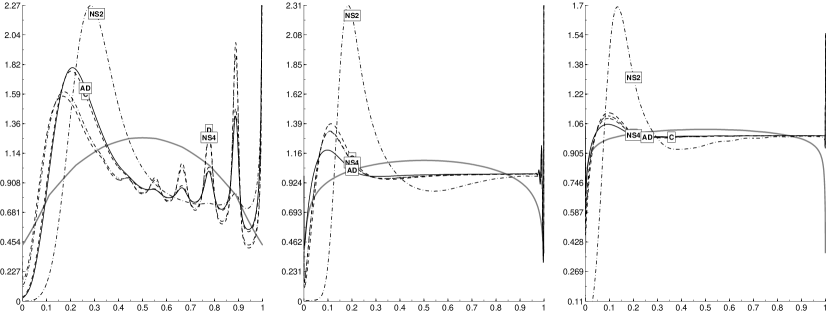
Bandwidths: NS2: 0.7446 C: 0.3496 NS4: 0.2528 D: 0.2355 AD:  0.3673	Bandwidths: NS2: 0.3149 C: 0.0904 NS4: 0.0787 D: 0.0796 AD:  0.0523	Bandwidths: NS2: 0.1405 C: 0.0338 NS4: 0.0363 D: 0.0399 AD:  0.0266

Figure 7: Marginal density of PITs for selected bandwidth values

#4: Kurtotic unimodal
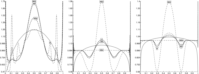
Bandwidths: NS2: 0.7414 C: 0.4362 NS4: 0.4418 D: 0.2419 AD:  0.6980	Bandwidths: NS2: 0.3113 C: 0.0993 NS4: 0.0091 D: 0.0958 AD:  0.0868	Bandwidths: NS2: 0.1400 C: 0.0407 NS4: 0.0010 D: 0.0539 AD:  0.0458
#5: Outlier
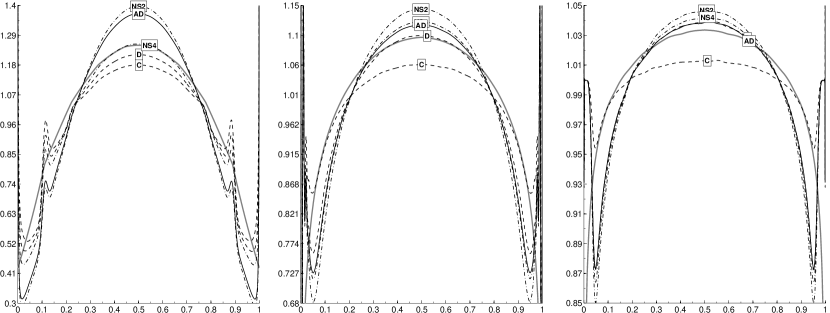
Bandwidths: NS2: 0.3331 C: 0.2250 NS4: 0.2664 D: 0.2457 AD:  0.3202	Bandwidths: NS2: 0.1700 C: 0.1042 NS4: 0.1569 D: 0.1418 AD:  0.1534	Bandwidths: NS2: 0.0944 C: 0.0496 NS4: 0.0894 D: 0.0863 AD:  0.0859
#6: Bimodal
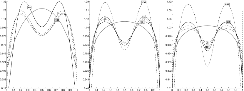
Bandwidths: NS2: 1.0421 C: 0.6762 NS4: 0.6422 D: 0.7477 AD:  1.0449	Bandwidths: NS2: 0.5532 C: 0.2825 NS4: 0.2875 D: 0.3207 AD:  0.3578	Bandwidths: NS2: 0.2923 C: 0.1270 NS4: 0.1554 D: 0.1838 AD:  0.1848

Figure 7 (Cont.): Marginal density of PITs for selected bandwidth values

4 Concluding remarks

This paper proposes a framework for choosing a single bandwidth for kernel estimators of both density and distribution functions motivated by the role of probability integral transforms in classical parametric modelling and their relationship to entropy maximisation. The leave-one-out estimates of a d.f. at sample values, $V_{i}$’s, are the analogues of PITs in parametric models. If the maximum entropy distribution were achieved, the $V_{i}$’s would be jointly uniformly distributed over the rescaled regular permutohedron $\Pi_{n}$. In general this cannot be achieved in finite sample, but the bandwidth can be chosen so that the distribution of $V_{i}$’s is close to the MaxEnt distribution. The proposed estimation procedures for the iMaxEnt bandwidth are fully operationalisable for finite $n$. Several estimators are examined in a simulation study, and the bandwidth minimising the Anderson-Darling version of the Cramér-von Mises discrepancy is found to perform reliably and—in a loose sense—robustly for a variety of distribution shapes.

Validity of Conjecture 1 remains an open question that further research could usefully address. If it holds, the resultant iMaxEnt bandwidth will be found to asymptotically occupy the in-between position relative to the KDE and KDFE MISE-minimising bandwidths, reinforcing the use of the iMaxEnt procedure as a unifying framework for kernel estimation of density and distribution functions. However, the absence of the proof is not a hindrance for the practical implementation of the proposed method in finite samples.

Appendices

Appendix A Uniform distribution over a regular permutohedron

A.1 Exact calculation of the marginal density

The expression for the marginal density given in Lemma 3 is exact but requires calculation of volume of certain permutohedra. The latter can be computed exactly using the following result due to Postnikov (2009, Theorem 3.1.). Suppose that $x_{1}>\cdots>x_{n}$, and let $\lambda_{1},\ldots,\lambda_{n}\in\mathbbm{R}$ be fixed distinct numbers. Then the volume of the permutohedron $P_{n}=P_{n}(x_{1},\ldots,x_{n})$ is equal to

$$\mathop{\mathrm{Vol}}\nolimits_{n-1}\left(P_{n}\right)=\frac{1}{(n-1)!}\sum_{\sigma\in S_{n}}\frac{\left(\lambda_{\sigma(1)}x_{1}+\cdots+\lambda_{\sigma(n)}x_{n}\right)^{n-1}}{(\lambda_{\sigma(1)}-\lambda_{\sigma(2)})(\lambda_{\sigma(2)}-\lambda_{\sigma(3)})\cdots(\lambda_{\sigma(n-1)}-\lambda_{\sigma(n)})},$$ (A.1)

where $S_{n}$ is the symmetric group. (See also Theorem 3.2 and section 16 in Postnikov (2009) for alternative expressions for the volume of permutohedra.) The $\lambda_{i}$’s in (A.1) cancel out and the resultant expression for $\mathop{\mathrm{Vol}}\nolimits_{n-1}\left(P_{n}\right)$ is a homogeneous polynomial of degree $n-1$ in $x_{1},\ldots,x_{n}$. For a given $n$, the marginal density (5) is then a piecewise $(n-2)$-degree polynomial on intervals $[(j-1)/(n-1),\;j/(n-1)]$, $j=1,\ldots,n-1$. For example, $l_{2}(u)=1$ if $u\in[0,1]$,

$$l_{3}(u)=\begin{cases}\frac{2}{3}\left(2u+1\right)&\;\text{if}\;u\in[0;1/2]\\ \frac{2}{3}\left(3-2u\right)&\;\text{if}\;u\in[1/2;1]\\ \end{cases}$$

$$l_{4}(u)=\begin{cases}\frac{3}{32}\left(9u^{2}+18u+6\right)&\;\text{if}\;u\in[0;1/3]\\ \frac{3}{32}\left(-18u^{2}+18u+9\right)&\;\text{if}\;u\in[1/3;2/3]\\ \frac{3}{32}\left(9u^{2}-36u+33\right)&\;\text{if}\;u\in[2/3;1]\\ \end{cases}$$

and so on.

A.2 Approximation of the marginal density by simulation

As $n$ increases, it quickly becomes impractical to use expression (A.1) as it involves summation over $n!$ permutations. One can then resort to numerical approximation of $l_{n}$ based on random draws from a uniform distribution over $\Pi_{n}$ which can be obtained using a simple rejection method. Specifically, draw random variates $u_{1},\ldots,u_{n-1}$ from a uniform distribution over a cube $I^{n-1}$, set $u_{n}=n/2-(u_{1}+\cdots+u_{n-1})$, and reject if $u=(u_{1},\ldots,u_{n})^{\mathsf{T}}\notin I^{n}$. The accepted draws are distributed uniformly over $I^{n}\cap H_{\boldsymbol{\iota}_{n},n/2}$, the central section of $I^{n}$. The draws are then rejected if $u\notin\Pi_{n}$ by calling a membership oracle.

The following result due to Rado (1952) requires only sorting to verify membership of $u$ in $\Pi_{n}$. This can be done only in $\mathit{O}\left(n\log n\right)$ operations. For any $x\in\mathbbm{R}^{n}$ let $x_{[1]}\geq\cdots\geq x_{[n]}$ denote the components of $x$ in decreasing order (reverse order statistics). Then for $x,y\in\mathbbm{R}^{n}$, $x$ is said to be majorized by $y$ ($y$ majorizes $x$), denoted as $x\prec y$ (or $y\succ x$), if

$$\sum_{i=1}^{k}x_{[i]}\leq\sum_{i=1}^{k}y_{[i]},\quad k=1,\ldots,n,$$

where there is equality with $k=n$. Furthermore, $x\prec y$ if and only if $x\in P_{n}(y)$. That is, to verify if $u\in\Pi_{n}$, one has only to verify if $u\in H_{\boldsymbol{\iota}_{n},n/2}$ is majorized by $(1,(n-2)/(n-1),(n-3)/(n-1),\ldots,1/(n-1),0)$. The overall acceptance rate of the above method is $\mathit{O}\left(n^{-1}\right)$.

The density $l_{n}$ and the corresponding d.f., moments, or any other functionals of $l_{n}$ can be approximated from the simulated data by the standard techniques.

Appendix B Sarda (1993) cross-validation criterion

Sarda (1993) proposed choosing the bandwidth for KDFE by minimising the following cross-validation (CV) criterion:

$$\operatorname{CV}_{\psi}(b)=n^{-1}\sum_{i=1}^{n}\left[V_{i}(b)-F_{n}(x_{i})\right]^{2}\psi(x_{i}),$$ (B.1)

where $\psi$ is a non-negative weight function. $\operatorname{CV}_{\psi}(b)$ is designed to approximate the weighted MISE

$$\operatorname{MISE}_{\psi}\widehat{F}(\cdot;b)=\operatorname{E}\int_{-\infty}^{\infty}\left[\widehat{F}(x;b)-F(x)\right]^{2}\psi(x)dF(x).$$

Summing in (B.1) over $i$ in the order of $x_{(i)}$ (see footnote 1), it can be seen that the CV criterion with $\psi(x)\equiv 1$ is computationally equivalent (up to an additive constant) to the classical CvM discrepancy between the EDF of $V$, $G_{n}$, and the uniform d.f. on $[0,1]$, $R$, viz. $\operatorname{CV}_{1}(b)=\omega^{2}(G_{n},R)+1/(6n^{2})$.

Lemma B.1

If Assumptions 1(a,b), 2(a,b), and 3 hold, then as $n\to\infty$ and $b\to 0$,

$$\begin{split}\omega^{2}(G,R)&=\frac{1}{4}\mu_{2}^{2}(k)\zeta_{1}(F)b^{4}-\frac{1}{2}\mu_{2}(k)R_{3}(f)b^{2}n^{-1}+\frac{1}{12}n^{-2}+\frac{1}{2}\mu_{2}(k)\psi_{2,1}(K)\zeta_{2}(F)b^{3}n^{-1}\\ &\quad-\psi_{2,1}(K)R_{2}(f)bn^{-2}+\mathit{O}\left(\max(b^{4}n^{-1},b^{6},b^{2}n^{-2},n^{-3})\right),\end{split}$$

where $R_{j}(f)=\int f(x)^{j}dx$, and $\zeta_{1}(F)$ and $\zeta_{1}(F)$ are constants depending on $F$ defined in (C.1). $\square$

In view of Lemma 2, one expects the bandwidth obtained by minimising a discrepancy between $G$ and the uniform distribution to be of order $n^{-1/2}$, which is indeed the same as the bandwidth minimising the two leading terms in $\omega^{2}(G,R)$. However, $\operatorname{E}\operatorname{CV}_{1}(b)=\omega^{2}(G,R)+\operatorname{IVar}G_{n}+1/(6n^{2})$, where $\operatorname{IVar}G_{n}=\int_{0}^{1}\operatorname{E}\left[G_{n}(t)-G(t)\right]^{2}dt$ is the integrated variance of $G_{n}$. This adds an extra term of order $b/n$, entering $\operatorname{E}\operatorname{CV}_{1}$ with a positive sign. This term dominates asymptotically and therefore $\operatorname{E}\operatorname{CV}_{1}$ is an increasing function of $b$, minimized by $b=0$. This provides an alternative confirmation of the failure of $\operatorname{CV}_{1}$ first pointed out in Altman and Léger (1995). In can be shown that the offending term is due to the correlation between $\mathbbm{1}\left\{V_{i}\leq t\right\}$ and $\mathbbm{1}\left\{V_{j}\leq t\right\}$, $i\neq j$.

Appendix C Proofs

Proof of Lemma 1. By Assumption 2(a), $K_{b}(0)=1/2$ and $K_{b}(-z)=1-K_{b}(z)$. Collecting the $\binom{n}{2}$ values of $\kappa_{ij}=K_{b}(X_{i}-X_{j})$, $i,j=1,\ldots,n$, $j>i$, in an $n(n-1)/2$-vector $\kappa=\left(\kappa_{12},\ldots,\kappa_{1n},\kappa_{23},\ldots,\kappa_{2n},\ldots,\kappa_{(n-1)n}\right)^{\mathsf{T}}$, the leave-one-out PITs (4), $V=(V_{1},\ldots,V_{n})^{\mathsf{T}}$, can be written as $(n-1)V+1=p(\kappa)=A(2\kappa-1)+(n+1)/2$, where $A=[a_{1},\ldots,a_{n(n-1)/2}]$ is an $n\times n(n-1)/2$ matrix with $a_{l}=(e_{i}-e_{j})/2$, $i=1,\ldots,n-1$, $j=i+1,\ldots,n$, where $e_{i},\ldots,e_{n}$ are the standard basis vectors in $\mathbbm{R}^{n}$.

Remark now that $2\kappa-1$ lies in the $n(n-1)/2$-cube $C^{n(n-1)/2}=[-1,1]^{n(n-1)/2}$, and the image of $C^{n(n-1)/2}$ under the affine projection $p(\kappa)$ is the permutohedron $P_{n}(1,2,\ldots,n)$; see Ziegler (1995, Sec.7.3). Therefore, the support of $V$ is $\Pi_{n}$, as required. $\blacksquare$

Proof of Lemma 2. If Assumptions 1(a,b) and 2(a,b) hold, then by an expansion around $x$ as $b\to 0$, for $r=1,2,\ldots$,

$$\begin{split}\operatorname{E}_{X_{1}}K_{b}^{r}(x-X_{1})&=\int_{-\infty}^{\infty}rK^{r-1}(z)k(z)F(x-bz)dz\\ &=F(x)-\psi_{r,1}(K)f(x)b+\frac{1}{2}\psi_{r,2}(K)f^{(1)}(x)b^{2}-\frac{1}{6}\psi_{r,3}(K)f^{(2)}(x)b^{3}+\mathit{O}\left(b^{4}\right),\end{split}$$

where for $j=0,1,2,\ldots$, $\psi_{r,j}(K)=\int_{-\infty}^{\infty}z^{j}rK^{r-1}(z)k(z)dz$; $\psi_{r,0}=1$ and $\psi_{1,j}=\mu_{j}(k)$, which is zero if $j$ is odd by symmetry of $k$. Then $\operatorname{E}_{X_{1}}K_{b}(x-X_{1})=F(x)+\frac{1}{2}\mu_{2}(k)f^{(1)}(x)b^{2}+\mathit{O}\left(b^{4}\right)$, and $\operatorname{E}_{X_{1}}K_{b}^{2}(x-X_{1})=F(x)-\psi_{2,1}(K)f(x)b+\mathit{O}\left(b^{2}\right)$. Thus, for $r\geq 2$,

$$\begin{split}\operatorname{E}V_{1}^{r}&=\int_{-\infty}^{\infty}\left[\frac{1}{(n-1)^{r}}\sum_{j_{1}=2}^{n}\cdots\sum_{j_{r}=2}^{n}\operatorname{E}_{X_{j_{1}},\ldots,X_{j_{r}}}\prod_{i=1}^{r}K_{b}(x-X_{j_{i}})\right]f(x)dx\\ &=\left[1-\binom{r}{2}n^{-1}\right]\int_{-\infty}^{\infty}\left[\operatorname{E}_{X_{1}}K_{b}(x-X_{1})\right]^{r}f(x)dx\\ &\qquad+n^{-1}\binom{r}{2}\int_{-\infty}^{\infty}\left[\operatorname{E}_{X_{1}}K_{b}(x-X_{1})\right]^{r-2}\left[\operatorname{E}_{X_{1}}K_{b}^{2}(x-X_{1})\right]f(x)dx+\mathit{O}\left(n^{-2}\right)\\ &=\frac{1}{r+1}-\frac{1}{2}\mu_{2}(k)\xi_{2,r}(F)b^{2}+\frac{r-1}{2(r+1)}n^{-1}-\psi_{2,1}(K)\xi_{1,r}(F)bn^{-1}+\mathit{O}\left(\max(b^{2}n^{-1},h^{4},n^{-2})\right),\end{split}$$

where $\xi_{2,r}(F)=-\int_{-\infty}^{\infty}rF^{r-1}(x)f^{(1)}(x)f(x)dx$ and $\xi_{1,r}(F)=\int_{-\infty}^{\infty}\frac{r(r-1)}{2}F^{r-2}(x)f^{2}(x)dx$. Furthermore, integration by parts yields $\xi_{2,r}(F)=\frac{r(r-1)}{2}\int_{-\infty}^{\infty}F^{r-2}(x)f^{3}(x)dx>0$. Finally, by Hölder’s inequality with exponents $1$ and $\infty$, $\xi_{2,r}(F)\leq\frac{r}{2}\sup_{x}f^{2}(x)$, and $\xi_{1,r}(F)\leq\frac{r}{2}\sup_{x}f(x)$. $\blacksquare$

Proof of Lemma 3. Since $\mathop{\mathrm{Vol}}\nolimits_{n-1}\left(\Pi_{n}\right)=n^{n-2}/(n-1)^{n-1}$, for $u\in[0,1]$, $l_{n}(u)=(n-1)^{n-1}\mathop{\mathrm{Vol}}\nolimits_{n-2}\left(\Pi_{n}\cap H_{e_{1},u}\right)/n^{n-2}$. Recognising that the sections $\Pi_{n}\cap H_{e_{1},u}$ are themselves permutohedra and applying Theorem 1 in Gaiha and Gupta (1977), we obtain for $u\in\left[\frac{j-1}{n-1},\frac{j}{n-1}\right]$, $j=1,\ldots,n-1$,

$$\Pi_{n}\cap H_{e_{1},u}=(n-1)^{-1}P_{n-1}(n-1,n-2,\ldots,j+1,2j-1-(n-1)u,j-2,\ldots,0),$$

which gives (5) as required. Noting that the sections $\Pi_{n}\cap H_{e_{1},0}$ and $\Pi_{n}\cap H_{e_{1},1}$ are translated copies of $\Pi_{n-1}$, one immediately obtains that the marginal density at $0$ and $1$ is $l_{n}(0)=l_{n}(1)=\left(1-1/n\right)^{n-2}\xrightarrow{n\to\infty}e^{-1}$. $\blacksquare$

Proof of Lemma B.1. Let $\rho_{r}(v)$, $r=0,1,2,\ldots$, be the shifted Legendre polynomials orthonormal with respect to the uniform density on the unit interval, viz. $\int_{0}^{1}\rho_{r}(v)\rho_{s}(v)dv=\delta_{rs}$, where $\delta_{rs}$ is the Kronecker delta (see footnote 2). Let $\rho_{r}^{(s)}(v)=\frac{d^{s}}{dv^{s}}\rho_{r}(v)$ for $s=0,1,2,\ldots$ denote the derivatives, and $\rho_{r}^{(-1)}(v)=\int_{0}^{v}\rho_{r}(t)dt$ be the first antiderivative of $\rho_{r}$. Then $q(v)$ can be expanded into a generalised Fourier series as $q(v)=1+\sum_{r=1}^{\infty}c_{r}\rho_{r}(v)$, where the coefficients are given by

$$c_{r}=\int_{0}^{1}\rho_{r}(v)g(v)dv=(-1)^{r}\sqrt{2r+1}\sum_{i=0}^{r}\binom{r}{i}\binom{r+i}{i}(-1)^{i}\operatorname{E}V_{1}^{i}.$$

Specifically, $c_{0}=1$, $c_{1}=0$, and for $r\geq 2$, $c_{r}=\sqrt{2r+1}\tilde{c}_{r}$, with

$$\tilde{c}_{r}=-\frac{1}{2}\mu_{2}(k)\tilde{\xi}_{2,r}(F)b^{2}+\mathbbm{1}\left\{r\;\text{even}\right\}n^{-1}-\psi_{2,1}(K)\tilde{\xi}_{1,r}(F)bn^{-1}+\mathit{O}\left(\max(b^{2}n^{-1},b^{4},n^{-2})\right),$$

where $\tilde{\xi}_{2,r}(F)=\frac{1}{2}\int_{-\infty}^{\infty}\frac{\rho_{r}^{(2)}\left(F(x)\right)}{\sqrt{2r+1}}f^{3}(x)dx=\int_{-\infty}^{\infty}\frac{\rho_{r}\left(F(x)\right)}{\sqrt{2r+1}}f^{(2)}(x)dx$ and $\tilde{\xi}_{1,r}(F)=\frac{1}{2}\int_{-\infty}^{\infty}\frac{\rho_{r}^{(2)}\left(F(x)\right)}{\sqrt{2r+1}}f^{2}(x)dx$. Note that $\tilde{\xi}_{2,2}(F)=6R_{3}(f)$ and $\tilde{\xi}_{1,2}(F)=6R_{2}(f)$.

Expanding $G(v)=v+\sum_{r=2}^{\infty}c_{r}\rho_{r}^{-1}(v)$ and using repeated integration by parts to find that for $n,m\geq 2$,

$$\sqrt{2n+1}\sqrt{2m+1}\int_{0}^{1}\rho_{n}^{(-1)}(v)\rho_{m}^{(-1)}(v)dv=\begin{cases}\frac{2n+1}{2(2n-1)(2n+3)}&\text{ if }n=m,\\ -\frac{1}{4(2n-1)}&\text{ if }\left|n-m\right|=2,\\ 0&\text{ otherwise},\end{cases}$$

yields

$$\begin{split}\omega^{2}(G,R)&=\sum_{r=2}^{\infty}\sum_{s=2}^{\infty}\tilde{c}_{r}\tilde{c}_{s}\sqrt{2r+1}\sqrt{2s+1}\int_{0}^{1}\rho_{r}^{-1}(v)\rho_{s}^{-1}(v)dv=\sum_{r=2}^{\infty}\left[\frac{(2r+1)\tilde{c}_{r}^{2}}{2(2r-1)(2r+3)}-\frac{\tilde{c}_{r}\tilde{c}_{r+2}}{2(2r+3)}\right]\\ &=\frac{1}{4}\mu_{2}^{2}(k)\zeta_{1}(F)b^{4}-\frac{1}{2}\mu_{2}(k)\theta_{1}b^{2}n^{-1}+\theta_{2}n^{-2}+\frac{1}{2}\mu_{2}(k)\psi_{2,1}(K)\zeta_{2}(F)b^{3}n^{-1}-\psi_{2,1}(K)\theta_{3}bn^{-2}\\ &\quad+\mathit{O}\left(\max(b^{4}n^{-1},b^{6},b^{2}n^{-2},n^{-3})\right),\end{split}$$

where

$$\begin{split}\zeta_{1}(F)&=\sum_{r=2}^{\infty}\left[\frac{(2r+1)}{2(2r-1)(2r+3)}\tilde{\xi}_{2,r}^{2}(F)-\frac{1}{2(2r+3)}\tilde{\xi}_{2,r}(F)\tilde{\xi}_{2,r+2}(F)\right],\\ \zeta_{2}(F)&=\sum_{r=2}^{\infty}\left[\frac{2(2r+1)}{2(2r-1)(2r+3)}\tilde{\xi}_{1,r}(F)\tilde{\xi}_{2,r}(F)-\frac{1}{2(2r+3)}\left(\tilde{\xi}_{1,r+2}(F)\tilde{\xi}_{2,r}(F)+\tilde{\xi}_{2,r+2}(F)\tilde{\xi}_{1,r}(F)\right)\right],\end{split}$$ (C.1)

$$\theta_{1}=\sum_{r=2}^{\infty}\left[\frac{\tilde{\xi}_{2,r}(F)}{2(2r-1)}-\frac{\tilde{\xi}_{2,r+2}(F)}{2(2r+3)}\right]\mathbbm{1}\left\{r\;\text{even}\right\}=\frac{1}{6}\tilde{\xi}_{2,2}(F)+\sum_{s=2}^{\infty}\frac{\tilde{\xi}_{2,2s}(F)}{2(4s-1)}-\sum_{s=1}^{\infty}\frac{\tilde{\xi}_{2,2(s+1)}(F)}{2(4(s+1)-1)}=R_{3}(f),$$

$$\theta_{2}=\sum_{r=2}^{\infty}\frac{\mathbbm{1}\left\{r\;\text{even}\right\}}{(2r-1)(2r+3)}=\sum_{s=1}^{\infty}\frac{1}{(4(s-1)+3)(4s+3)}=\frac{1}{12},$$

$$\theta_{3}=\sum_{r=2}^{\infty}\left[\frac{\tilde{\xi}_{1,r}(F)}{2(2r-1)}-\frac{\tilde{\xi}_{1,r+2}(F)}{2(2r+3)}\right]\mathbbm{1}\left\{r\;\text{even}\right\}=\frac{1}{6}\tilde{\xi}_{1,2}(F)+\sum_{s=2}^{\infty}\frac{\tilde{\xi}_{1,2s}(F)}{2(4s-1)}-\sum_{s=1}^{\infty}\frac{\tilde{\xi}_{1,2(s+1)}(F)}{2(4(s+1)-1)}=R_{2}(f),$$

as required $\blacksquare$

Appendix D Beta-weighted Cramér–von Mises criteria

Let $\omega_{\alpha,\beta;\epsilon}^{2}$ denote the CvM discrepancy (6) with $\psi(t)=t^{\alpha-1}(1-t)^{\beta-1}\mathbbm{1}\left\{\epsilon\leq t\leq 1-\epsilon\right\}$, $\alpha,\beta\geq 0$, $0\leq\epsilon<1/2$, and let $B(x;\alpha,\beta)=\int_{0}^{x}t^{\alpha-1}(1-t)^{\beta-1}dt$ and $B(\alpha,\beta)=B(1;\alpha,\beta)$ denote the incomplete and complete beta functions, respectively. Let $U_{i}=F(Z_{i})$ and $u_{(1)}\leq\cdots\leq u_{(n)}$ be the respective order statistics with $u_{(0)}\equiv 0$ and $u_{(n+1)}\equiv 1$. Then in view of the second equality in (6) and because $G_{n}\circ F^{-1}$ is the EDF of $U$, unless $\alpha=\beta=0$,

$$\omega_{\alpha,\beta;\epsilon}^{2}=\sum_{j=0}^{n}\int_{u_{(j)}}^{u_{(j+1)}}\left[\frac{j}{n}-t\right]^{2}\psi(t)dt=\frac{1}{n}\sum_{j=j_{min}}^{j_{max}}\left[2B(u_{(j)};\alpha+1,\beta)-\frac{2j-1}{n}B(u_{(j)};\alpha,\beta)\right]+A_{\alpha,\beta;\epsilon},$$ (D.1)

where $j_{min}$ is the smallest index $j=1,\ldots,n$ such that $u_{(j_{min})}\geq\epsilon$, $j_{max}$ is the greatest index such that $u_{(j_{max})}\leq 1-\epsilon$, $u_{(j_{min}-1)}\equiv\epsilon$, $u_{(j_{max}+1)}\equiv 1-\epsilon$, and

$$\begin{split}A_{\alpha,\beta;\epsilon}&=\int_{0}^{1-\epsilon}\left[t-\frac{j_{max}}{n}\right]^{2}t^{\alpha-1}(1-t)^{\beta-1}dt-\int_{0}^{\epsilon}\left[t-\frac{j_{min}-1}{n}\right]^{2}t^{\alpha-1}(1-t)^{\beta-1}dt.\\ &=B(1-\epsilon;\alpha+2,\beta)-B(\epsilon;\alpha+2,\beta)\\ &\qquad-\frac{2j_{max}}{n}B(1-\epsilon;\alpha+1,\beta)+\frac{2(j_{min}-1)}{n}B(\epsilon;\alpha+1,\beta)+\frac{j_{max}^{2}}{n^{2}}B(1-\epsilon;\alpha,\beta)-\frac{(j_{min}-1)^{2}}{n^{2}}B(\epsilon;\alpha,\beta).\end{split}$$

When there is no trimming ($\epsilon=0$), $j_{min}=1$, $j_{max}=n$, and $A_{\alpha,\beta;\epsilon}=B(\alpha,\beta+2)$. Another special case of interest is the trimmed classical CvM when $\alpha=\beta=1$, viz.

$$\omega_{1,1;\epsilon}^{2}=\frac{1}{n}\sum_{j=j_{min}}^{j_{max}}\left[u_{(j)}-\frac{2j-1}{2n}\right]^{2}+\frac{j_{max}-j_{min}+1}{12n^{3}}+\frac{1}{3}\left(1-\epsilon-\frac{j_{max}}{n}\right)^{3}-\frac{1}{3}\left(\epsilon-\frac{j_{min}-1}{n}\right)^{3}.$$

(When $\epsilon=0$ the second term becomes $1/(12n^{2})$ and the last two terms are zero).

For the case $\alpha=\beta=0$ (Anderson-Darling criterion) and $\epsilon>0$ we have

$$\begin{split}\omega_{0,0;\epsilon}^{2}&=\frac{1}{n}\sum_{j=j_{min}}^{j_{max}}\left[-2\ln(1-u_{(j)})-\frac{2j-1}{n}\left(\ln(u_{(j)})-\ln(1-u_{(j)})\right)\right]\\ &\qquad-1+2\epsilon+\left[\frac{j_{max}^{2}}{n^{2}}+\left(\frac{j_{min}-1}{n}-1\right)^{2}\right]\ln(1-\epsilon)-\left[\left(\frac{j_{max}}{n}-1\right)^{2}+\frac{(j_{min}-1)^{2}}{n^{2}}\right]\ln(\epsilon).\end{split}$$

With $\epsilon=0$, $\omega_{AD}^{2}=\omega_{0,0;0}^{2}=-\frac{1}{n^{2}}\sum_{j=1}^{n}(2j-1)\left[\ln(u_{(j)})+\ln(1-u_{(n-j+1)})\right]-1$.

Supplement to ‘Indirect Maximum Entropy Bandwidth’ Vitaliy Oryshchenko^$\ast$
University of Manchester

Appendix S.1 $2^{\text{nd}}$—$10^{\text{th}}$ even central moments of a random variable with density $l_{n}(u)$ for $n=2,\ldots,1,000,000$

Tables S.1.2–S.1.5 list values of the first five even central moments of a random variable with density $l_{n}(u)$ for $n$ between $2$ and $1,000,000$. The values for $n=2,\ldots,11$ are exact. For $12\leq n\leq 100,000$, the values are obtained by simulation from $\left\lceil 1e5\times n\right\rceil/1e4$ random draws from a uniform distribution on $\Pi_{n}$ and exploiting the fact that all marginals are identical. For $n=177,828,\;316,228,\;562,341$, and $1,000,000$ the number of random draws is $6000,\;4000,\;900$, and $500$, respectively.

The values in the tables are displayed as $m_{2}\times 1e5$, $m_{4}\times 1e6$, $m_{6}\times 1e6$, $m_{8}\times 1e7$, and $m_{10}\times 1e8$, rounded to a nearest integer. For example, for $n=2$, $m_{2}\approx 0.08333$, $m_{4}\approx 0.012500$, $m_{6}\approx 0.002232$, $m_{8}\approx 0.0004340$, and $m_{10}\approx 0.00008878$.

Figure S.1.1 plots the moments against $n$ (on a log-scale). In each case the following regression was estimated on subsamples $n\geq 10$, $n\geq 100$, $n\geq 1,000$, $n\geq 10,000$:

$$\log_{10}\left(\hat{m}_{2k}-m_{2k,0}\right)=\alpha+\beta\log_{10}(n),\quad k=1,\ldots,5,$$ (S.1.1)

where $\hat{m}_{2k}$ are the tabulated moments of a random variable with density $l_{n}(u)$ and $m_{2k,0}$ are the central moments of a uniform random variable on $[0,1]$. The estimates are given in Table S.1.1. The constants shown in Figure S.1.1 are determined by restricting $\beta=-1/2$ in (S.1.1) and using the subsample $n\geq 10,000$.

Table S.1.1: Regression fit for the marginal even central moments of a random variable distributed uniformly on the permutohedron $\Pi_{n}$

	Estimates of $\beta$ in (S.1.1)				Estimates of $10^{\alpha}$ in (S.1.1)
$2k$	$n\geq 10$	$n\geq 100$	$n\geq 1,000$	$n\geq 10,000$	$n\geq 10$	$n\geq 100$	$n\geq 1,000$	$n\geq 10,000$
2	-0.4512	-0.4748	-0.4896	-0.4944	0.0677	0.0814	0.0927	0.0974
4	-0.4388	-0.4677	-0.4868	-0.4942	0.0151	0.0189	0.0224	0.0242
6	-0.4288	-0.4619	-0.4844	-0.4935	0.0032	0.0042	0.0051	0.0056
8	-0.4204	-0.4569	-0.4823	-0.4927	0.0007	0.0009	0.0012	0.0013
10	-0.4131	-0.4525	-0.4804	-0.4921	0.0002	0.0002	0.0003	0.0003

These finite sample results motivate the conjecture that as $n\to\infty$, the marginal moments of a random variable distributed uniformly on the permutohedron $\Pi_{n}$ approach the respective moments of the uniform random variable on $[0,1]$ from below at a rate $n^{-1/2}$.

Table S.1.2: Central moments of $l_{n}$, $n=2,\ldots,99$

$n$	$m_{2}$	$m_{4}$	$m_{6}$	$m_{8}$	$m_{10}$	$n$	$m_{2}$	$m_{4}$	$m_{6}$	$m_{8}$	$m_{10}$
2	8333	12500	2232	4340	8878	51	7202	9864	1648	3041	5957
3	6944	9722	1674	3183	6412	52	7211	9881	1652	3048	5973
4	6597	8912	1504	2824	5642	53	7219	9899	1655	3056	5989
5	6483	8609	1434	2670	5300	54	7226	9915	1659	3063	6004
6	6451	8493	1404	2596	5129	55	7234	9932	1662	3070	6020
7	6452	8460	1391	2562	5042	56	7242	9948	1665	3077	6034
8	6469	8468	1388	2548	5000	57	7249	9963	1669	3084	6049
9	6494	8497	1391	2546	4986	58	7256	9979	1672	3091	6064
10	6522	8537	1396	2552	4988	59	7263	9993	1675	3097	6077
11	6552	8584	1403	2562	5001	60	7270	10009	1678	3104	6092
12	6582	8634	1411	2575	5022	61	7276	10023	1681	3111	6106
13	6611	8684	1419	2589	5046	62	7283	10037	1684	3117	6119
14	6640	8735	1428	2604	5073	63	7289	10051	1687	3123	6132
15	6667	8785	1437	2620	5102	64	7296	10065	1690	3129	6144
16	6694	8834	1446	2636	5132	65	7302	10079	1693	3135	6158
17	6719	8882	1454	2652	5162	66	7308	10093	1696	3141	6171
18	6744	8928	1463	2669	5194	67	7314	10106	1698	3147	6184
19	6767	8973	1471	2685	5225	68	7320	10118	1701	3153	6196
20	6790	9016	1480	2700	5255	69	7326	10130	1704	3158	6207
21	6811	9058	1487	2716	5285	70	7331	10143	1706	3164	6220
22	6832	9099	1495	2731	5315	71	7337	10155	1709	3169	6231
23	6852	9138	1503	2745	5345	72	7342	10167	1711	3174	6242
24	6871	9176	1510	2760	5373	73	7348	10179	1714	3180	6254
25	6889	9213	1517	2774	5402	74	7353	10191	1716	3185	6265
26	6907	9248	1524	2788	5430	75	7358	10202	1719	3190	6276
27	6924	9282	1531	2801	5456	76	7363	10213	1721	3195	6287
28	6940	9315	1537	2814	5483	77	7368	10224	1723	3200	6298
29	6956	9347	1544	2827	5509	78	7373	10234	1726	3205	6308
30	6971	9379	1550	2839	5535	79	7378	10245	1728	3210	6319
31	6986	9408	1556	2851	5559	80	7383	10256	1730	3214	6329
32	7000	9437	1562	2863	5583	81	7387	10266	1732	3219	6339
33	7014	9466	1567	2874	5607	82	7392	10276	1734	3223	6349
34	7027	9493	1573	2885	5630	83	7396	10287	1737	3228	6359
35	7040	9520	1578	2896	5652	84	7401	10297	1739	3233	6369
36	7052	9546	1583	2907	5675	85	7406	10307	1741	3237	6379
37	7064	9571	1588	2917	5697	86	7410	10316	1743	3242	6388
38	7076	9596	1593	2927	5718	87	7414	10325	1745	3246	6398
39	7087	9620	1598	2937	5738	88	7418	10335	1747	3250	6407
40	7099	9643	1603	2947	5759	89	7422	10344	1749	3255	6416
41	7109	9665	1607	2956	5778	90	7426	10353	1751	3259	6425
42	7119	9687	1612	2966	5798	91	7430	10362	1753	3263	6434
43	7130	9709	1616	2975	5817	92	7435	10371	1755	3267	6443
44	7140	9731	1621	2984	5836	93	7438	10380	1756	3271	6452
45	7150	9751	1625	2993	5854	94	7442	10388	1758	3275	6460
46	7159	9771	1629	3001	5873	95	7446	10397	1760	3279	6469
47	7168	9791	1633	3010	5890	96	7450	10405	1762	3283	6478
48	7177	9810	1637	3018	5908	97	7453	10414	1764	3286	6486
49	7186	9828	1641	3026	5925	98	7457	10422	1766	3290	6495
50	7195	9847	1645	3033	5941	99	7460	10429	1767	3294	6502

Table S.1.3: Central moments of $l_{n}$, $n=100,\ldots,1,000$

$n$	$m_{2}$	$m_{4}$	$m_{6}$	$m_{8}$	$m_{10}$	$n$	$m_{2}$	$m_{4}$	$m_{6}$	$m_{8}$	$m_{10}$
100	7465	10438	1769	3298	6510	320	7807	11223	1940	3674	7345
102	7472	10454	1772	3305	6527	327	7812	11235	1943	3680	7358
105	7482	10476	1777	3315	6549	335	7817	11248	1946	3686	7373
107	7488	10491	1780	3322	6564	343	7823	11261	1949	3693	7388
110	7498	10513	1785	3332	6586	351	7828	11273	1951	3699	7402
112	7504	10527	1788	3339	6600	359	7833	11286	1954	3705	7415
115	7513	10547	1792	3348	6621	368	7839	11298	1957	3711	7430
118	7521	10567	1796	3357	6641	376	7844	11310	1960	3717	7443
120	7527	10579	1799	3363	6654	385	7849	11322	1962	3723	7456
123	7536	10598	1803	3372	6674	394	7854	11334	1965	3729	7470
126	7544	10617	1807	3381	6693	404	7859	11347	1968	3736	7485
129	7551	10634	1811	3389	6710	413	7864	11358	1970	3741	7497
132	7559	10651	1815	3397	6729	423	7869	11370	1973	3747	7511
135	7566	10667	1818	3405	6745	433	7874	11382	1976	3753	7524
138	7573	10684	1822	3412	6762	443	7879	11393	1978	3759	7537
142	7582	10704	1826	3422	6784	453	7883	11404	1981	3764	7549
145	7589	10719	1829	3429	6799	464	7888	11416	1983	3770	7563
148	7595	10734	1833	3436	6815	475	7893	11427	1986	3776	7576
152	7604	10753	1837	3445	6834	486	7898	11439	1988	3782	7589
156	7612	10771	1841	3454	6855	498	7903	11450	1991	3787	7602
159	7618	10785	1844	3460	6868	509	7907	11460	1993	3792	7614
163	7625	10802	1848	3469	6887	521	7911	11470	1996	3798	7626
167	7632	10819	1851	3477	6904	534	7916	11482	1998	3804	7639
171	7640	10835	1855	3484	6922	546	7920	11491	2000	3808	7650
175	7647	10852	1858	3492	6939	559	7925	11503	2003	3814	7663
179	7653	10866	1862	3499	6955	572	7929	11513	2005	3819	7675
183	7660	10881	1865	3507	6971	586	7934	11524	2008	3825	7687
187	7666	10896	1868	3514	6987	599	7938	11533	2010	3830	7699
192	7673	10913	1872	3522	7005	614	7942	11543	2012	3835	7709
196	7679	10927	1875	3528	7020	628	7946	11554	2014	3840	7721
201	7686	10942	1878	3536	7037	643	7950	11564	2017	3845	7733
206	7693	10959	1882	3544	7055	658	7955	11573	2019	3850	7744
210	7699	10971	1885	3550	7068	673	7958	11583	2021	3855	7756
215	7705	10987	1888	3558	7085	689	7963	11593	2023	3860	7767
221	7713	11004	1892	3566	7104	705	7967	11602	2025	3865	7778
226	7719	11018	1895	3573	7119	722	7970	11611	2027	3870	7789
231	7725	11032	1898	3580	7134	739	7974	11621	2030	3875	7800
236	7731	11045	1901	3586	7148	756	7978	11630	2032	3879	7811
242	7737	11060	1904	3594	7165	774	7982	11639	2034	3884	7822
248	7744	11075	1908	3601	7181	792	7986	11649	2036	3889	7833
254	7750	11090	1911	3608	7197	811	7990	11658	2038	3893	7843
260	7756	11104	1914	3615	7213	830	7993	11667	2040	3898	7853
266	7761	11117	1917	3621	7227	850	7997	11676	2042	3903	7865
272	7767	11130	1920	3628	7242	870	8001	11684	2044	3907	7875
278	7773	11143	1922	3634	7256	890	8004	11693	2046	3911	7884
285	7779	11158	1926	3641	7272	911	8008	11702	2048	3916	7895
292	7785	11172	1929	3648	7288	933	8012	11710	2050	3920	7905
298	7790	11183	1931	3654	7301	955	8015	11719	2052	3925	7915
305	7795	11196	1934	3660	7315	977	8019	11727	2054	3929	7925
313	7802	11211	1938	3668	7332	1000	8022	11735	2055	3933	7934

Table S.1.4: Central moments of $l_{n}$, $n=1,000,\ldots,10,000$

$n$	$m_{2}$	$m_{4}$	$m_{6}$	$m_{8}$	$m_{10}$	$n$	$m_{2}$	$m_{4}$	$m_{6}$	$m_{8}$	$m_{10}$
1000	8022	11735	2055	3933	7934	3199	8155	12058	2129	4102	8324
1024	8025	11744	2057	3938	7945	3275	8157	12062	2130	4105	8329
1048	8029	11751	2059	3942	7954	3352	8158	12067	2132	4107	8335
1072	8032	11759	2061	3946	7963	3430	8161	12072	2133	4110	8341
1097	8035	11767	2063	3950	7973	3511	8163	12077	2134	4113	8347
1123	8038	11775	2065	3954	7982	3594	8164	12082	2135	4115	8353
1150	8041	11783	2066	3958	7991	3678	8166	12086	2136	4117	8358
1177	8045	11791	2068	3962	8001	3765	8168	12091	2137	4120	8364
1205	8048	11798	2070	3966	8010	3854	8170	12096	2138	4122	8370
1233	8051	11806	2072	3970	8019	3944	8172	12101	2139	4125	8376
1262	8054	11813	2073	3974	8028	4037	8174	12105	2140	4127	8381
1292	8057	11821	2075	3977	8036	4132	8175	12109	2141	4129	8387
1322	8060	11828	2077	3982	8045	4229	8177	12113	2142	4132	8391
1353	8063	11835	2078	3985	8054	4329	8179	12117	2143	4134	8396
1385	8066	11843	2080	3989	8063	4431	8181	12122	2144	4136	8402
1417	8069	11849	2082	3993	8071	4535	8183	12126	2145	4139	8408
1451	8072	11857	2083	3997	8080	4642	8184	12130	2146	4141	8412
1485	8075	11864	2085	4000	8088	4751	8186	12134	2147	4143	8417
1520	8078	11871	2086	4004	8096	4863	8188	12139	2148	4145	8423
1556	8081	11877	2088	4007	8105	4977	8189	12143	2149	4147	8428
1592	8083	11884	2089	4011	8112	5094	8191	12147	2150	4149	8433
1630	8086	11891	2091	4014	8120	5214	8192	12150	2151	4152	8438
1668	8089	11898	2093	4018	8129	5337	8194	12154	2152	4153	8442
1707	8092	11904	2094	4021	8136	5462	8195	12158	2152	4155	8447
1748	8095	11911	2096	4025	8145	5591	8197	12162	2153	4157	8452
1789	8097	11917	2097	4028	8153	5722	8199	12166	2154	4160	8457
1831	8099	11923	2098	4031	8159	5857	8200	12170	2155	4162	8461
1874	8102	11930	2100	4035	8167	5995	8202	12174	2156	4164	8466
1918	8105	11936	2101	4038	8174	6136	8203	12177	2157	4166	8470
1963	8107	11942	2103	4041	8183	6280	8204	12180	2158	4167	8474
2009	8110	11948	2104	4044	8189	6428	8206	12184	2159	4169	8479
2057	8112	11955	2106	4048	8198	6579	8207	12187	2159	4171	8484
2105	8115	11960	2107	4051	8205	6734	8209	12191	2160	4173	8488
2154	8117	11966	2108	4054	8211	6893	8210	12195	2161	4175	8492
2205	8120	11972	2110	4057	8219	7055	8212	12198	2162	4177	8496
2257	8122	11978	2111	4060	8225	7221	8213	12201	2163	4179	8501
2310	8124	11983	2112	4063	8233	7391	8214	12205	2163	4181	8505
2364	8126	11989	2113	4066	8239	7565	8216	12208	2164	4182	8509
2420	8129	11995	2115	4069	8246	7743	8217	12211	2165	4184	8513
2477	8131	12000	2116	4072	8253	7925	8219	12215	2166	4186	8517
2535	8133	12005	2117	4075	8260	8111	8220	12218	2166	4188	8521
2595	8135	12011	2118	4077	8265	8302	8221	12221	2167	4189	8525
2656	8138	12016	2120	4080	8273	8498	8222	12224	2168	4191	8529
2719	8140	12022	2121	4083	8279	8697	8223	12226	2168	4192	8532
2783	8142	12028	2122	4086	8287	8902	8225	12230	2169	4194	8536
2848	8144	12032	2124	4089	8292	9112	8226	12233	2170	4196	8540
2915	8146	12038	2125	4092	8299	9326	8227	12236	2171	4197	8544
2984	8149	12043	2126	4094	8305	9545	8228	12239	2171	4199	8547
3054	8151	12048	2127	4097	8311	9770	8230	12243	2172	4201	8552
3126	8153	12053	2128	4100	8318	10000	8231	12246	2173	4203	8556

Table S.1.5: Central moments of $l_{n}$, $n=12,589,\ldots,1,000,000$

$n$	$m_{2}$	$m_{4}$	$m_{6}$	$m_{8}$	$m_{10}$	$n$	$m_{2}$	$m_{4}$	$m_{6}$	$m_{8}$	$m_{10}$
12589	8242	12273	2179	4217	8589	63096	8292	12397	2208	4284	8746
15849	8252	12297	2185	4230	8620	79433	8296	12408	2211	4290	8761
19953	8260	12318	2190	4241	8647	100000	8300	12418	2213	4296	8773
25119	8268	12338	2194	4252	8672	177828	8308	12438	2218	4307	8799
31623	8275	12355	2198	4261	8693	316228	8315	12454	2221	4315	8819
39811	8281	12371	2202	4270	8713	562341	8319	12465	2224	4321	8834
50119	8287	12385	2205	4278	8731	1000000	8323	12474	2226	4326	8844

(a) $2^{\text{nd}}$ central moment

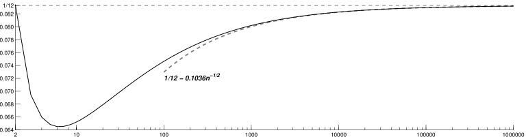
(b) $4^{\text{th}}$ central moment

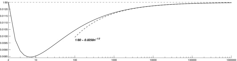
(c) $6^{\text{th}}$ central moment

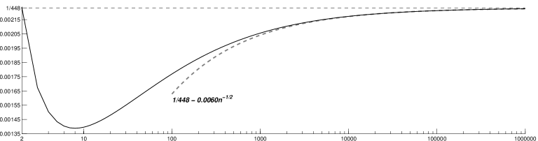
(d) $8^{\text{th}}$ central moment

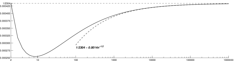
(e) $10^{\text{th}}$ central moment

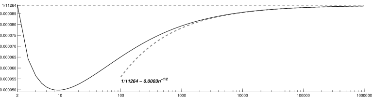
Horizontal axes: sample size, $n$, log-scale.

Black line—central moments of $U_{i}$; dashed grey line—$a_{j,n}=m_{j,0}-c_{j}n^{-1/2}$, where $m_{j,0}$ are the $j^{th}$ central moments of the uniform distribution, and constants $c_{j}$ are determined numerically.

Figure S.1.1: Even central moments of $U_{i}$ and asymptotic fit

Appendix S.2 Additional Monte Carlo results

Tables S.2.1–S.2.6 list the $0$, $0.025$, $0.25$, $0.5$, $0.75$, $0.975$, and $1^{st}$ quantiles (denoted as min, $2.5^{th}$-p., $1^{st}$ Q., median, $3^{rd}$ Q., $97.5^{th}$-p., and max, respectively), as well as the sample average and standard deviation of the simulated distribution of selected bandwidth estimators for sample sizes $10$, $100$, and $1,000$. The estimators are: minimum Neyman Smooth Test (min-Neyman Sm.) estimators using the first $k=2$, $3$, or $4$ polynomials; the moment-based estimators (MEE) based on the first $m=2$, $3$, and $4$ moments; and the minimum weighted Cramér-von Mises estimators with the weight function $\psi(t)=t^{\alpha-1}(1-t)^{\alpha-1}\mathbbm{1}\left\{\epsilon\leq t\leq 1-\epsilon\right\}$ for $\alpha=0$ (the Anderson-Darling criterion), $1/4$, and $1/2$, and $\epsilon=0.001$.

Table S.2.1: Performance of iMaxEnt bandwidth estimators: Density #1 (Gaussian)

	min-Neyman Sm.			MEE (CUE)			min-CvM
	$k=2$	$k=3$	$k=4$	$m=2$	$m=3$	$m=4$	$\alpha=0$	$\alpha=1/4$	$\alpha=1/2$
$n=10$; min-MISE bandwidths: 0.6495 (KCDFE), 0.7585 (KDE).
min	0.0969	0.0000	0.0000	0.1591	0.1329	0.0000	0.0609	0.0001	0.0000
$2.5^{th}$-p.	0.4605	0.2117	0.2155	0.4988	0.4074	0.1090	0.4247	0.3368	0.1985
$1^{st}$ Q.	0.7580	0.6359	0.5319	0.7734	0.6914	0.4785	0.8161	0.7582	0.6949
median	0.9374	0.8828	0.7915	0.9350	0.8601	0.7193	1.0091	0.9674	0.9262
$3^{rd}$ Q.	1.1260	1.1140	1.0366	1.1009	1.0369	0.9777	1.1982	1.1657	1.1433
$97.5^{th}$-p.	1.5279	1.5389	1.4991	1.4542	1.4050	1.5845	1.5854	1.5696	1.5631
max	1.9337	2.0041	2.3252	1.8648	1.8544	2.5339	2.0393	2.0875	2.0204
avg.	0.9510	0.8745	0.8005	0.9454	0.8712	0.7456	1.0090	0.9623	0.9105
st.dev.	0.2726	0.3460	0.3456	0.2449	0.2556	0.3765	0.2891	0.3083	0.3432
$n=100$; min-MISE bandwidths: 0.3147 (KCDFE), 0.4455 (KDE).
min	0.3319	0.2294	0.0180	0.3380	0.3379	0.0620	0.0325	0.0000	0.0000
$2.5^{th}$-p.	0.4084	0.3678	0.3226	0.4165	0.4108	0.3354	0.3600	0.3272	0.2734
$1^{st}$ Q.	0.4628	0.4436	0.4291	0.4668	0.4626	0.4442	0.4386	0.4268	0.4168
median	0.4931	0.4776	0.4687	0.4949	0.4911	0.4805	0.4712	0.4629	0.4562
$3^{rd}$ Q.	0.5231	0.5104	0.5060	0.5231	0.5191	0.5154	0.5008	0.4961	0.4922
$97.5^{th}$-p.	0.5832	0.5734	0.5735	0.5771	0.5738	0.5819	0.5576	0.5556	0.5565
max	0.6654	0.6577	0.6822	0.6666	0.6627	0.7046	0.6366	0.6416	0.6468
avg.	0.4936	0.4759	0.4635	0.4955	0.4911	0.4756	0.4677	0.4579	0.4475
st.dev.	0.0442	0.0514	0.0642	0.0411	0.0417	0.0620	0.0512	0.0595	0.0734
$n=1000$; min-MISE bandwidths: 0.1517 (KCDFE), 0.2723 (KDE).
min	0.2447	0.2400	0.2271	0.2448	0.2447	0.2311	0.2246	0.2092	0.1939
$2.5^{th}$-p.	0.2566	0.2541	0.2522	0.2569	0.2567	0.2554	0.2456	0.2391	0.2329
$1^{st}$ Q.	0.2667	0.2647	0.2678	0.2667	0.2664	0.2695	0.2588	0.2546	0.2507
median	0.2717	0.2703	0.2740	0.2716	0.2714	0.2753	0.2648	0.2617	0.2586
$3^{rd}$ Q.	0.2768	0.2756	0.2798	0.2766	0.2763	0.2808	0.2705	0.2680	0.2655
$97.5^{th}$-p.	0.2867	0.2857	0.2903	0.2861	0.2859	0.2909	0.2804	0.2790	0.2771
max	0.3004	0.3000	0.3023	0.2995	0.2994	0.3024	0.2944	0.2938	0.2936
avg.	0.2717	0.2702	0.2734	0.2716	0.2713	0.2748	0.2644	0.2609	0.2576
st.dev.	0.0076	0.0080	0.0095	0.0074	0.0074	0.0089	0.0089	0.0102	0.0115

Table S.2.2: Performance of iMaxEnt bandwidth estimators: Density #2 (Skewed unimodal)

	min-Neyman Sm.			MEE (CUE)			min-CvM
	$k=2$	$k=3$	$k=4$	$m=2$	$m=3$	$m=4$	$\alpha=0$	$\alpha=1/4$	$\alpha=1/2$
$n=10$; min-MISE bandwidths: 0.5896 (KCDFE), 0.6602 (KDE).
min	0.1763	0.0000	0.0000	0.2014	0.0772	0.0000	0.0455	0.0000	0.0000
$2.5^{th}$-p.	0.4025	0.1658	0.1935	0.4388	0.3590	0.1052	0.3667	0.2980	0.1737
$1^{st}$ Q.	0.6860	0.5250	0.4822	0.7083	0.6171	0.4557	0.7062	0.6472	0.5849
median	0.8636	0.7536	0.7095	0.8726	0.7772	0.6834	0.9145	0.8610	0.8100
$3^{rd}$ Q.	1.0614	0.9872	0.9573	1.0604	0.9610	0.9375	1.1354	1.0772	1.0333
$97.5^{th}$-p.	1.5016	1.4683	1.4505	1.4538	1.3567	1.5366	1.5682	1.5241	1.4975
max	2.2357	2.2825	2.6780	2.0919	1.9552	2.6282	2.4228	2.2569	2.2912
avg.	0.8872	0.7650	0.7373	0.8942	0.8004	0.7158	0.9301	0.8725	0.8136
st.dev.	0.2820	0.3373	0.3384	0.2606	0.2550	0.3670	0.3085	0.3141	0.3356
$n=100$; min-MISE bandwidths: 0.2764 (KCDFE), 0.3743 (KDE).
min	0.2923	0.1658	0.0000	0.3073	0.2814	0.0200	0.0000	0.0000	0.0000
$2.5^{th}$-p.	0.3635	0.2659	0.2446	0.3717	0.3559	0.2637	0.2845	0.2529	0.2045
$1^{st}$ Q.	0.4170	0.3503	0.3493	0.4229	0.4059	0.3919	0.3671	0.3545	0.3433
median	0.4465	0.3913	0.3955	0.4513	0.4339	0.4307	0.4034	0.3949	0.3874
$3^{rd}$ Q.	0.4774	0.4298	0.4372	0.4804	0.4619	0.4655	0.4373	0.4306	0.4251
$97.5^{th}$-p.	0.5385	0.4963	0.5085	0.5379	0.5182	0.5312	0.4975	0.4947	0.4919
max	0.6364	0.5868	0.6008	0.6222	0.6005	0.6355	0.5678	0.5717	0.5752
avg.	0.4475	0.3887	0.3900	0.4522	0.4344	0.4237	0.4000	0.3896	0.3786
st.dev.	0.0444	0.0593	0.0687	0.0421	0.0418	0.0649	0.0553	0.0620	0.0730
$n=1000$; min-MISE bandwidths: 0.1317 (KCDFE), 0.2257 (KDE).
min	0.2154	0.1649	0.1638	0.2161	0.2089	0.1788	0.1727	0.1638	0.1388
$2.5^{th}$-p.	0.2303	0.1882	0.1949	0.2310	0.2233	0.2241	0.2000	0.1941	0.1882
$1^{st}$ Q.	0.2403	0.2046	0.2123	0.2407	0.2333	0.2387	0.2151	0.2112	0.2076
median	0.2454	0.2130	0.2211	0.2457	0.2384	0.2446	0.2218	0.2185	0.2155
$3^{rd}$ Q.	0.2505	0.2212	0.2292	0.2507	0.2435	0.2504	0.2281	0.2253	0.2229
$97.5^{th}$-p.	0.2604	0.2357	0.2444	0.2603	0.2530	0.2609	0.2398	0.2376	0.2359
max	0.2732	0.2516	0.2619	0.2728	0.2636	0.2753	0.2529	0.2573	0.2502
avg.	0.2454	0.2128	0.2207	0.2457	0.2383	0.2441	0.2213	0.2179	0.2147
st.dev.	0.0077	0.0122	0.0125	0.0075	0.0076	0.0093	0.0100	0.0110	0.0120

Table S.2.3: Performance of iMaxEnt bandwidth estimators: Density #3 (Strongly skewed)

	min-Neyman Sm.			MEE (CUE)			min-CvM
	$k=2$	$k=3$	$k=4$	$m=2$	$m=3$	$m=4$	$\alpha=0$	$\alpha=1/4$	$\alpha=1/2$
$n=10$; min-MISE bandwidths: 0.3496 (KCDFE), 0.2355 (KDE).
min	0.0033	0.0000	0.0000	0.0611	0.0418	0.0000	0.0007	0.0000	0.0000
$2.5^{th}$-p.	0.2310	0.0019	0.0580	0.2523	0.1440	0.0158	0.0628	0.0352	0.0009
$1^{st}$ Q.	0.5177	0.1025	0.1507	0.5313	0.3299	0.1542	0.2035	0.1576	0.0986
median	0.7446	0.2329	0.2528	0.7424	0.4890	0.2922	0.3673	0.3057	0.2414
$3^{rd}$ Q.	1.0080	0.4991	0.4251	0.9806	0.7002	0.4692	0.7009	0.5741	0.4881
$97.5^{th}$-p.	1.5372	1.2927	0.9154	1.4364	1.1893	0.8705	1.3658	1.2358	1.0910
max	2.3178	2.1789	1.6234	2.0319	1.8464	1.4259	2.0109	2.0164	1.8115
avg.	0.7832	0.3564	0.3171	0.7691	0.5378	0.3330	0.4870	0.4064	0.3293
st.dev.	0.3443	0.3489	0.2260	0.3115	0.2763	0.2291	0.3638	0.3256	0.2971
$n=100$; min-MISE bandwidths: 0.0904 (KCDFE), 0.0796 (KDE).
min	0.1361	0.0264	0.0335	0.1336	0.0861	0.0336	0.0000	0.0000	0.0000
$2.5^{th}$-p.	0.2234	0.0399	0.0489	0.2135	0.1233	0.0505	0.0039	0.0000	0.0000
$1^{st}$ Q.	0.2805	0.0573	0.0667	0.2675	0.1622	0.0700	0.0394	0.0237	0.0000
median	0.3149	0.0700	0.0787	0.2991	0.1863	0.0834	0.0523	0.0407	0.0001
$3^{rd}$ Q.	0.3522	0.0853	0.0922	0.3341	0.2134	0.0992	0.0655	0.0567	0.0229
$97.5^{th}$-p.	0.4294	0.1281	0.1272	0.4049	0.2751	0.1423	0.0972	0.0919	0.0816
max	0.5524	0.2304	0.1936	0.5244	0.3800	0.2147	0.1697	0.1673	0.1607
avg.	0.3178	0.0733	0.0810	0.3020	0.1896	0.0866	0.0527	0.0408	0.0138
st.dev.	0.0529	0.0226	0.0201	0.0493	0.0385	0.0233	0.0214	0.0249	0.0250
$n=1000$; min-MISE bandwidths: 0.0338 (KCDFE), 0.0399 (KDE).
min	0.1119	0.0250	0.0273	0.1068	0.0601	0.0299	0.0000	0.0000	0.0000
$2.5^{th}$-p.	0.1256	0.0291	0.0315	0.1206	0.0702	0.0343	0.0200	0.0103	0.0000
$1^{st}$ Q.	0.1352	0.0322	0.0346	0.1297	0.0765	0.0378	0.0245	0.0208	0.0000
median	0.1405	0.0339	0.0363	0.1348	0.0800	0.0397	0.0266	0.0236	0.0000
$3^{rd}$ Q.	0.1459	0.0358	0.0382	0.1400	0.0837	0.0418	0.0287	0.0263	0.0182
$97.5^{th}$-p.	0.1566	0.0395	0.0418	0.1501	0.0910	0.0460	0.0327	0.0327	0.0253
max	0.1791	0.0457	0.0472	0.1719	0.1058	0.0519	0.0379	0.0368	0.0366
avg.	0.1406	0.0340	0.0364	0.1349	0.0802	0.0398	0.0265	0.0232	0.0084
st.dev.	0.0079	0.0027	0.0026	0.0076	0.0054	0.0030	0.0033	0.0055	0.0097

Table S.2.4: Performance of iMaxEnt bandwidth estimators: Density #4 (Kurtotic unimodal)

	min-Neyman Sm.			MEE (CUE)			min-CvM
	$k=2$	$k=3$	$k=4$	$m=2$	$m=3$	$m=4$	$\alpha=0$	$\alpha=1/4$	$\alpha=1/2$
$n=10$; min-MISE bandwidths: 0.4362 (KCDFE), 0.2419 (KDE).
min	0.0478	0.0000	0.0000	0.0667	0.0596	0.0000	0.0000	0.0000	0.0000
$2.5^{th}$-p.	0.1998	0.0682	0.0009	0.2558	0.1821	0.0481	0.1012	0.0703	0.0072
$1^{st}$ Q.	0.5128	0.2729	0.1590	0.5968	0.5044	0.3983	0.3318	0.2468	0.1650
median	0.7414	0.5510	0.4418	0.8105	0.7274	0.7922	0.6980	0.5072	0.3404
$3^{rd}$ Q.	0.9893	0.8701	0.8649	1.0381	0.9695	1.1740	1.0586	0.9220	0.7430
$97.5^{th}$-p.	1.5106	1.4689	1.4905	1.5072	1.4355	1.9674	1.6003	1.5006	1.3734
max	2.2317	2.2405	2.5601	2.1840	2.1644	3.0406	2.3337	2.3306	2.3325
avg.	0.7682	0.6061	0.5437	0.8288	0.7468	0.8270	0.7248	0.6051	0.4786
st.dev.	0.3423	0.3915	0.4396	0.3218	0.3301	0.5223	0.4348	0.4167	0.3882
$n=100$; min-MISE bandwidths: 0.0993 (KCDFE), 0.0958 (KDE).
min	0.1334	0.0945	0.0000	0.1494	0.1493	0.0000	0.0000	0.0000	0.0000
$2.5^{th}$-p.	0.2009	0.1715	0.0000	0.2233	0.2199	0.0001	0.0001	0.0000	0.0000
$1^{st}$ Q.	0.2698	0.2479	0.0035	0.2976	0.2941	0.0138	0.0678	0.0646	0.0614
median	0.3113	0.2943	0.0091	0.3394	0.3362	0.0271	0.0868	0.0829	0.0797
$3^{rd}$ Q.	0.3576	0.3434	0.0209	0.3854	0.3821	0.0436	0.1077	0.1016	0.0979
$97.5^{th}$-p.	0.4499	0.4377	0.0738	0.4726	0.4703	0.5694	0.1914	0.1654	0.1524
max	0.5760	0.5754	0.6515	0.5884	0.5876	0.8544$(^{*}$	0.5693	0.5473	0.3918
avg.	0.3150	0.2970	0.0177	0.3417	0.3384	0.0555$(^{*}$	0.0901	0.0837	0.0787
st.dev.	0.0634	0.0688	0.0350	0.0636	0.0640	0.1209$(^{*}$	0.0455	0.0394	0.0369
$n=1000$; min-MISE bandwidths: 0.0407 (KCDFE), 0.0539 (KDE).
min	0.1071	0.1070	0.0000	0.1100	0.1100	0.0014	0.0000	0.0000	0.0000
$2.5^{th}$-p.	0.1223	0.1210	0.0003	0.1255	0.1254	0.0020	0.0340	0.0326	0.0315
$1^{st}$ Q.	0.1338	0.1324	0.0008	0.1373	0.1371	0.0024	0.0424	0.0413	0.0406
median	0.1400	0.1389	0.0010	0.1436	0.1434	0.0026	0.0458	0.0447	0.0439
$3^{rd}$ Q.	0.1466	0.1455	0.0013	0.1503	0.1502	0.0029	0.0490	0.0478	0.0471
$97.5^{th}$-p.	0.1598	0.1590	0.0022	0.1637	0.1635	0.0036	0.0550	0.0536	0.0527
max	0.1821	0.1761	0.0044	0.1864	0.1855	0.0066	0.0626	0.0609	0.0597
avg.	0.1403	0.1391	0.0011	0.1439	0.1437	0.0027	0.0455	0.0443	0.0435
st.dev.	0.0095	0.0096	0.0005	0.0097	0.0097	0.0004	0.0056	0.0056	0.0057

$(^{*}$– without one extreme value of $\hat{b}$ ($1.62e7$).

Table S.2.5: Performance of iMaxEnt bandwidth estimators: Density #5 (Outlier)

	min-Neyman Sm.			MEE (CUE)			min-CvM
	$k=2$	$k=3$	$k=4$	$m=2$	$m=3$	$m=4$	$\alpha=0$	$\alpha=1/4$	$\alpha=1/2$
$n=10$; min-MISE bandwidths: 0.2250 (KCDFE), 0.2457 (KDE).
min	0.0640	0.0000	0.0000	0.0615	0.0396	0.0000	0.0035	0.0001	0.0000
$2.5^{th}$-p.	0.1577	0.0686	0.0606	0.1718	0.1429	0.0315	0.1208	0.1003	0.0652
$1^{st}$ Q.	0.2637	0.2063	0.1808	0.2766	0.2412	0.1637	0.2550	0.2362	0.2169
median	0.3331	0.2889	0.2664	0.3517	0.3094	0.2515	0.3202	0.3056	0.2937
$3^{rd}$ Q.	0.4203	0.3708	0.3506	0.4562	0.3944	0.3530	0.3957	0.3829	0.3699
$97.5^{th}$-p.	0.7102	0.5808	0.5321	0.9540	0.8014	0.7970	0.6231	0.5659	0.5309
max	2.1502	1.9930	1.8215	2.9251	3.2072	6.3076	2.6660	1.5242	0.9372
avg.	0.3591	0.2956	0.2713	0.3993	0.3461	0.3044	0.3356	0.3134	0.2942
st.dev.	0.1559	0.1362	0.1250	0.2111	0.1920	0.3517	0.1374	0.1188	0.1172
$n=100$; min-MISE bandwidths: 0.1042 (KCDFE), 0.1418 (KDE).
min	0.1103	0.0831	0.0018	0.1129	0.1116	0.0105	0.0000	0.0000	0.0000
$2.5^{th}$-p.	0.1385	0.1256	0.0749	0.1433	0.1414	0.0715	0.1108	0.1008	0.0894
$1^{st}$ Q.	0.1588	0.1518	0.1385	0.1637	0.1619	0.1317	0.1412	0.1374	0.1340
median	0.1700	0.1641	0.1569	0.1753	0.1734	0.1531	0.1534	0.1506	0.1481
$3^{rd}$ Q.	0.1822	0.1772	0.1717	0.1878	0.1862	0.1693	0.1652	0.1629	0.1609
$97.5^{th}$-p.	0.2068	0.2025	0.1985	0.2135	0.2119	0.1974	0.1874	0.1857	0.1844
max	0.2482	0.2483	0.2381	0.2602	0.2588	0.2295	0.2204	0.2190	0.2186
avg.	0.1709	0.1642	0.1524	0.1762	0.1745	0.1480	0.1524	0.1489	0.1457
st.dev.	0.0174	0.0195	0.0298	0.0179	0.0180	0.0311	0.0196	0.0216	0.0239
$n=1000$; min-MISE bandwidths: 0.0496 (KCDFE), 0.0863 (KDE).
min	0.0825	0.0816	0.0492	0.0832	0.0832	0.0484	0.0657	0.0573	0.0500
$2.5^{th}$-p.	0.0885	0.0877	0.0728	0.0892	0.0891	0.0700	0.0782	0.0759	0.0740
$1^{st}$ Q.	0.0924	0.0917	0.0843	0.0930	0.0929	0.0819	0.0834	0.0820	0.0807
median	0.0944	0.0938	0.0894	0.0950	0.0949	0.0872	0.0859	0.0847	0.0835
$3^{rd}$ Q.	0.0964	0.0959	0.0935	0.0971	0.0970	0.0917	0.0882	0.0870	0.0861
$97.5^{th}$-p.	0.1004	0.0999	0.0996	0.1011	0.1010	0.0985	0.0922	0.0913	0.0906
max	0.1055	0.1053	0.1057	0.1063	0.1062	0.1047	0.0975	0.0962	0.0960
avg.	0.0944	0.0938	0.0885	0.0951	0.0950	0.0864	0.0857	0.0844	0.0832
st.dev.	0.0030	0.0031	0.0070	0.0030	0.0030	0.0074	0.0036	0.0039	0.0042

Table S.2.6: Performance of iMaxEnt bandwidth estimators: Density #6 (Bimodal)

	min-Neyman Sm.			MEE (CUE)			min-CvM
	$k=2$	$k=3$	$k=4$	$m=2$	$m=3$	$m=4$	$\alpha=0$	$\alpha=1/4$	$\alpha=1/2$
$n=10$; min-MISE bandwidths: 0.6762 (KCDFE), 0.7477 (KDE).
min	0.1650	0.0000	0.0000	0.2074	0.1339	0.0000	0.0299	0.0135	0.0000
$2.5^{th}$-p.	0.5363	0.1650	0.1791	0.5699	0.4130	0.0605	0.3304	0.2530	0.0503
$1^{st}$ Q.	0.8782	0.6794	0.4048	0.8565	0.7416	0.3118	0.8568	0.7935	0.7134
median	1.0421	1.0104	0.6422	0.9936	0.9079	0.5619	1.0449	1.0253	1.0051
$3^{rd}$ Q.	1.2075	1.2247	0.8900	1.1333	1.0648	0.7828	1.2094	1.2073	1.2034
$97.5^{th}$-p.	1.5158	1.5642	1.3381	1.3894	1.3447	1.2107	1.5034	1.5182	1.5239
max	1.9962	2.0315	2.2831	1.7784	1.7643	1.9298	2.0276	2.0825	2.0183
avg.	1.0383	0.9370	0.6683	0.9908	0.8988	0.5669	1.0066	0.9724	0.9256
st.dev.	0.2478	0.3888	0.3192	0.2075	0.2379	0.3102	0.2966	0.3338	0.3877
$n=100$; min-MISE bandwidths: 0.2825 (KCDFE), 0.3207 (KDE).
min	0.4091	0.1820	0.1426	0.4101	0.3491	0.1374	0.0000	0.0000	0.0000
$2.5^{th}$-p.	0.4845	0.3212	0.2002	0.4707	0.4468	0.1963	0.2129	0.1394	0.0000
$1^{st}$ Q.	0.5302	0.4869	0.2529	0.5100	0.4994	0.2518	0.3051	0.2754	0.2185
median	0.5532	0.5291	0.2875	0.5298	0.5221	0.2883	0.3578	0.3419	0.3129
$3^{rd}$ Q.	0.5753	0.5598	0.3288	0.5496	0.5436	0.3320	0.4084	0.4110	0.4142
$97.5^{th}$-p.	0.6154	0.6070	0.4316	0.5865	0.5817	0.4318	0.4857	0.4987	0.5129
max	0.6771	0.6744	0.5466	0.6388	0.6360	0.5404	0.5651	0.5944	0.5889
avg.	0.5523	0.5137	0.2948	0.5296	0.5202	0.2959	0.3556	0.3387	0.2989
st.dev.	0.0335	0.0700	0.0585	0.0295	0.0345	0.0606	0.0728	0.0955	0.1444
$n=1000$; min-MISE bandwidths: 0.1270 (KCDFE), 0.1838 (KDE).
min	0.2695	0.2138	0.1229	0.2641	0.2552	0.1230	0.1321	0.0848	0.0000
$2.5^{th}$-p.	0.2815	0.2660	0.1388	0.2760	0.2745	0.1387	0.1632	0.1509	0.1318
$1^{st}$ Q.	0.2886	0.2836	0.1495	0.2828	0.2819	0.1494	0.1774	0.1685	0.1558
median	0.2923	0.2891	0.1554	0.2865	0.2857	0.1553	0.1848	0.1776	0.1670
$3^{rd}$ Q.	0.2958	0.2935	0.1615	0.2899	0.2893	0.1614	0.1921	0.1869	0.1784
$97.5^{th}$-p.	0.3026	0.3010	0.1747	0.2965	0.2960	0.1744	0.2063	0.2046	0.2004
max	0.3109	0.3107	0.1955	0.3043	0.3042	0.1957	0.2299	0.2341	0.2294
avg.	0.2922	0.2877	0.1557	0.2863	0.2855	0.1556	0.1847	0.1777	0.1669
st.dev.	0.0054	0.0088	0.0091	0.0052	0.0055	0.0091	0.0110	0.0137	0.0176

References

- (1)
- Akaike (1973) Akaike, H. (1973), Information theory and an extension of the maximum likelihood principle, in B. N. Petrov and F. Caski, eds, ‘Proceedings of the Second International Symposium on Information Theory’, Akademiai Kiado, pp. 267–281.
- Altman and Léger (1995) Altman, N. and Léger, C. (1995), ‘Bandwidth selection for kernel distribution function estimation’, Journal of Statistical Planning and Inference 46(2), 195–214. doi: 10.1016/0378-3758(94)00102-2
- Anderson and Darling (1952) Anderson, T. W. and Darling, D. A. (1952), ‘Asymptotic theory of certain “goodness of fit” criteria based on stochastic processes’, Annals of Mathematical Statistics 23(2), 193–212. doi: 10.1214/aoms/1177729437
- Bera and Ghosh (2002) Bera, A. K. and Ghosh, A. (2002), Neyman’s smooth test and its applications in econometrics, in A. Ullah, A. T. Wan and A. Chaturvedi, eds, ‘Handbook of Applied Econometrics and Statistical Inference’, Vol. 165 of Statistics: textbooks and monographs, Marcel Dekker, chapter 10, pp. 177–230.
- Chen (1999) Chen, S. X. (1999), ‘Beta kernel estimators for density functions’, Computational Statistics & Data Analysis 31(2), 131–145. doi: 10.1016/S0167-9473(99)00010-9
- Dawid (1984) Dawid, A. P. (1984), ‘Statistical theory: The prequential approach’, Journal of the Royal Statistical Society. Series A (General) 147(2), 278–292. doi: 10.2307/2981683
- Devroye and Györfi (1985) Devroye, L. and Györfi, L. (1985), Nonparametric Density Estimation: The View, John Wiley & Sons.
- Diebold et al. (1998) Diebold, F. X., Gunther, T. A. and Tay, A. S. (1998), ‘Evaluating density forecasts, with applications to financial risk management’, International Economic Review 39, 863–883. doi: 10.2307/2527342
- Gaiha and Gupta (1977) Gaiha, P. and Gupta, S. K. (1977), ‘Adjacent vertices on a permutohedron’, SIAM Journal on Applied Mathematics 32(2), 323–327. doi: 10.1137/0132025
- Gneiting et al. (2007) Gneiting, T., Balabdaoui, F. and Raftery, A. E. (2007), ‘Probabilistic forecasts, calibration and sharpness’, Journal of the Royal Statistical Society: Series B (Statistical Methodology) 69(2), 243–268. doi: 10.1111/j.1467-9868.2007.00587.x
- Hall (1987) Hall, P. (1987), ‘On Kullback–Leibler loss and density estimation’, Annals of Statistics 15(4), 1491–1519. doi: 10.1214/aos/1176350606
- Kanazawa (1993) Kanazawa, Y. (1993), ‘Hellinger distance and Kullback–Leibler loss for the kernel density estimator’, Statistics & Probability Letters 18(4), 315–321. doi: 10.1016/0167-7152(93)90022-B
- Marron and Wand (1992) Marron, J. S. and Wand, M. P. (1992), ‘Exact mean integrated squared error’, Annals of Statistics 20(2), 712–736. doi: 10.1214/aos/1176348653
- Nadaraya (1964) Nadaraya, E. A. (1964), ‘Some new estimates for distribution functions’, Theory of Probability and its Applications 9(3), 497–500. doi: 10.1137/1109069
- Newey and Smith (2004) Newey, W. K. and Smith, R. J. (2004), ‘Higher order properties of GMM and generalized empirical likelihood estimators’, Econometrica 72(1), 219–255. doi: 10.1111/j.1468-0262.2004.00482.x
- Neyman (1937) Neyman, J. (1937), “‘Smooth test” for goodness of fit’, Skandinavisk Aktuarietidskrift 20, 149–199. doi: 10.1080/03461238.1937.10404821
- Olver et al. (2010) Olver, F. W. J., Lozier, D. W., Boisvert, R. F. and Clark, C. W., eds (2010), NIST Handbook of Mathematical Functions, Cambridge University Press, New York, NY.
- Oryshchenko (2016) Oryshchenko, V. (2016), Exact mean integrated squared error of kernel distribution function estimators, preprint, arXiv: 1606.06993 [stat.ME]. URL: http://arxiv.org/abs/1606.06993
- Parzen (1962) Parzen, E. (1962), ‘On estimation of a probability density function and mode’, Annals of Mathematical Statistics 33(3), 1065–1076. doi: 10.1214/aoms/1177704472
- Postnikov (2009) Postnikov, A. (2009), ‘Permutohedra, associahedra, and beyond’, International Mathematics Research Notices 2009(6), 1026–1106. doi: 10.1093/imrn/rnn153
- Rado (1952) Rado, R. (1952), ‘An inequality’, Journal of The London Mathematical Society 27(1), 1–6. doi: 10.1112/jlms/s1-27.1.1
- Rosenblatt (1952) Rosenblatt, M. (1952), ‘Remarks on a multivariate transformation’, Annals of Mathematical Statistics 23(3), 470–472. doi: 10.1214/aoms/1177729394
- Rosenblatt (1956) Rosenblatt, M. (1956), ‘Remarks on some nonparametric estimates of a density function’, Annals of Mathematical Statistics 27(3), 832–837. doi: 10.1214/aoms/1177728190
- Sarda (1993) Sarda, P. (1993), ‘Smoothing parameter selection for smooth distribution functions’, Journal of Statistical Planning and Inference 35(1), 65–75. doi: 10.1016/0378-3758(93)90068-H
- Shao and Hahn (1994) Shao, Y. and Hahn, M. G. (1994), Maximum spacing estimates: A generalization and improvement on maximum likelihood estimates, in J. Hoffmann-Jørgensen, J. Kuelbs and M. B. Marcus, eds, ‘Probability in Banach Spaces, 9’, Vol. 35 of Progress in Probability, Boston: Birkhäuser, pp. 417–431. doi: 10.1007/978-1-4612-0253-0
- Silverman (1978) Silverman, B. W. (1978), ‘Weak and strong uniform consistency of the kernel estimate of a density and its derivatives’, Annals of Statistics 6(1), 177–184. doi: 10.1214/aos/1176344076
- Smirnov (1937) Smirnov, N. V. (1937), ‘On the distribution of the criterion of von Mises’, Matematicheskii Sbornik 2(44)(5), 973–993. (In Russian). URL: http://mi.mathnet.ru/rus/msb/v44/i5/p973
- Wand and Jones (1995) Wand, M. P. and Jones, M. C. (1995), Kernel Smoothing, Vol. 60 of Monographs on Statistics and Applied Probability, Chapman & Hall.
- Watson and Leadbetter (1964) Watson, G. S. and Leadbetter, M. R. (1964), ‘Hazard analysis II’, Sankhyā: The Indian Journal of Statistics, Series A 26(1), 101–116. URL: http://www.jstor.org/stable/25049316
- White (1982) White, H. (1982), ‘Maximum likelihood estimation of misspecified models’, Econometrica 50(1), 1–25.
- Yamato (1973) Yamato, H. (1973), ‘Uniform convergence of an estimator of a distribution function’, Bulletin of Mathematical Statistics 15(3-4), 69–78. URL: http://ci.nii.ac.jp/naid/120001036895/
- Ziegler (1995) Ziegler, G. M. (1995), Lectures on Polytopes, Vol. 152 of Graduate Texts in Mathematics, Springer. doi: 10.1007/978-1-4613-8431-1