Composing Scalable Nonlinear Algebraic Solvers

Abstract

Most efficient linear solvers use composable algorithmic components, with the most common model being the combination of a Krylov accelerator and one or more preconditioners. A similar set of concepts may be used for nonlinear algebraic systems, where nonlinear composition of different nonlinear solvers may significantly improve the time to solution. We describe the basic concepts of nonlinear composition and preconditioning and present a number of solvers applicable to nonlinear partial differential equations. We have developed a software framework in order to easily explore the possible combinations of solvers. We show that the performance gains from using composed solvers can be substantial compared with gains from standard Newton-Krylov methods.

1 Introduction

Large-scale algebraic solvers for nonlinear partial differential equations (PDEs) are an essential component of modern simulations. Newton-Krylov methods [23] have well-earned dominance. They are generally robust and may be built from preexisting linear solvers and preconditioners, including fast multilevel preconditioners such as multigrid [5, 7, 9, 67, 73] and domain decomposition methods [55, 63, 64, 66]. Newton’s method starts from whole-system linearization. The linearization leads to a large sparse linear system where the matrix may be represented either explicitly by storing the nonzero coefficients or implicitly by various “matrix-free” approaches [11, 42]. However, Newton’s method has a number of drawbacks as a stand-alone solver. The repeated construction and solution of the linearization cause memory bandwidth and communication bottlenecks to come to the fore with regard to performance. Also possible is a lack of convergence robustness when the initial guess is far from the solution. Luckily, a large design space for nonlinear solvers exists to complement, improve, or replace Newton’s method. Only a small part of this space has yet been explored either experimentally or theoretically.

In this paper we consider a wide collection of solvers for nonlinear equations. In direct equivalence to the case of linear solvers, we use a small number of algorithmic building blocks to produce a vast array of solvers with different convergence and performance properties. Two related solver techniques, nonlinear composition and preconditioning, are be used to construct these solvers. The contributions of this paper are twofold: introduction of a systematic approach to combining nonlinear solvers mathematically and in software and demonstration of the construction of efficient solvers for several problems of interest. Implementations of the solvers in this paper are available in the PETSc library and may be brought to bear on relevant applications, whether simulated on a laptop or on a supercomputer.

2 Background

We concern ourselves with the solution of nonlinear equations of the form

$$\mathbf{F}(\mathbf{x})=\mathbf{b}$$ (2.1)

for a general discretized nonlinear function $\mathbf{F}:\mathbb{R}^{n}\rightarrow\mathbb{R}^{n}$ and right hand side (RHS) $\mathbf{b}$. We define the nonlinear residual as

$$\mathbf{r}(\mathbf{x})=\mathbf{F}(\mathbf{x})-\mathbf{b}.$$ (2.2)

We retain both notations as certain solvers (Section 5.3) require the RHS to be modified. We will use

$$\mathbf{J}(\mathbf{x})=\frac{\partial\mathbf{F}(\mathbf{x})}{\partial\mathbf{x}}$$ (2.3)

to denote the Jacobian of $\mathbf{F}(\mathbf{x})$.

The linear system

$$\mathbf{A}\mathbf{x}=\mathbf{b}$$

with residual

$$\mathbf{r}(\mathbf{x})=\mathbf{A}\mathbf{x}-\mathbf{b}$$

is an important special case from which we can derive valuable insight into solvers for the nonlinear problem. Stationary solvers for linear systems repeatedly apply a linear operator in order to progressively improve the solution. The application of a linear stationary solver by defect correction may be written as

$$\mathbf{x}_{i+1}=\mathbf{x}_{i}-\mathbf{P}^{-1}\left(\mathbf{A}\mathbf{x}_{i}-\mathbf{b}\right),$$ (2.4)

where $\mathbf{P}^{-1}$ is a linear operator, called a preconditioner, whose action approximates, in some sense, the inverse of $\mathbf{A}$. The Jacobi, Gauss-Seidel, and multigrid iterations are all examples of linear stationary solvers.

composition of linear preconditioners $\mathbf{P}^{-1}$ and $\mathbf{Q}^{-1}$ may proceed in two different ways, producing two new stationary solvers. The first is the additive combination

$$\mathbf{x}_{i+1}=\mathbf{x}_{i}-\left(\alpha_{\mathbf{P}}\mathbf{P}^{-1}+\alpha_{\mathbf{Q}}\mathbf{Q}^{-1}\right)\left(\mathbf{A}\mathbf{x}_{i}-\mathbf{b}\right),$$

with weights $\alpha_{\mathbf{P}}$ and $\alpha_{\mathbf{Q}}$. The second is the multiplicative combination

$$\mathbf{x}_{i+1/2} = \mathbf{x}_{i}-\mathbf{P}^{-1}\left(\mathbf{A}\mathbf{x}_{i}-\mathbf{b}\right)$$

$$\mathbf{x}_{i+1} = \mathbf{x}_{i+1/2}-\mathbf{Q}^{-1}\left(\mathbf{A}\mathbf{x}_{i+1/2}-\mathbf{b}\right).$$

compositions consisting of $\mathbf{P}^{-1}$ and $\mathbf{Q}^{-1}$ are an effective acceleration strategy if $\mathbf{P}^{-1}$ eliminates a portion of the error space and $\mathbf{Q}^{-1}$ handles the rest. A now mature theory for these compositions was developed in the 1980s and 1990s in the context of domain decomposition methods [62, 66].

Linear left- and right-preconditioning, when used in conjunction with Krylov iterative methods [58], is standard practice for the parallel solution of linear systems of equations. We write the use of a linear Krylov method as $\text{K}(\mathbf{A},\mathbf{x},\mathbf{b}),$ where $\mathbf{A}$ is the matrix, $\mathbf{x}$ the initial solution, and $\mathbf{b}$ the RHS.

Linear left-preconditioning recasts the problem as

$$\mathbf{P}^{-1}(\mathbf{A}\mathbf{x}-\mathbf{b})=0,$$

while right-preconditioning takes two stages,

$$\mathbf{A}\mathbf{P}^{-1}\mathbf{y}=\mathbf{b}$$

$$\mathbf{P}^{-1}\mathbf{y}=\mathbf{x},$$

where one solves for the preconditioned solution $\mathbf{y}$ and then transforms $\mathbf{y}$ using $\mathbf{P}^{-1}$ to the solution of the original problem.

3 Nonlinear Composed Solvers

We take the basic patterns from the previous section and apply them to the nonlinear case. We emphasize that unlike the linear case, the nonlinear case requires the approximate solution as well as the residual to be defined both in the outer solver and in the preconditioner. With this in mind, we will show how composition and preconditioning may be systematically transferred to the nonlinear case.

We use the notation $\mathbf{x}_{i+1}=\mathbf{M}(\mathbf{r},\mathbf{x}_{i})$ for the action of a nonlinear solver. In most cases, but not always, $\mathbf{r}=\mathbf{r}(\mathbf{x}_{i})$, that is, $\mathbf{r}$ is simply the most recent residual. It is also useful to consider the action of a solver that is dependent on the previous $m$ approximate solutions and the previous $m$ residuals and as $\mathbf{x}_{i+1}=\mathbf{M}(\mathbf{r},\mathbf{x}_{i-m+1},\cdots,\mathbf{x}_{i},\mathbf{r}_{i-m+1},\cdots,\mathbf{r}_{i})$. Methods that store and use information from previous iterations such as previous solutions, residuals, or step directions will have those listed in the per-iteration inputs as well.

Nonlinear composition consists of a sequence or series of two (or more) solution methods $\mathbf{M}$ and $\mathbf{N}$, which both provide an approximate solution to (2.1). Nonlinear preconditioning, on the other hand, may be cast as a modification of the residual $\mathbf{r}$ through application of an inner method $\mathbf{N}$. The modified residual is then provided to an outer solver $\mathbf{M},$ which solves the preconditioned system.

An additive composition may be written as

$$\mathbf{x}_{i+1}=\mathbf{x}_{i}+\alpha_{\mathbf{M}}\left(\mathbf{M}(\mathbf{r},\mathbf{x}_{i})-\mathbf{x}_{i}\right)+\alpha_{\mathbf{N}}\left(\mathbf{N}(\mathbf{r},\mathbf{x}_{i})-\mathbf{x}_{i}\right)$$ (3.1)

for weights $\alpha_{\mathbf{M}}$ and $\alpha_{\mathbf{N}}$. The multiplicative composition is

$$\mathbf{x}_{i+1}=\mathbf{M}(\mathbf{r},\mathbf{N}(\mathbf{r},\mathbf{x}_{i}))=\mathbf{M}(\mathbf{r}(\mathbf{N}(\mathbf{r}(\mathbf{x}_{i}),\mathbf{x}_{i}),\mathbf{N}(\mathbf{r}(\mathbf{x}_{i}),\mathbf{x}_{i})),$$ (3.2)

which simply states: update the solution using the current solution and residual with the first solver and then update the solution again using the resulting new solution and new residual with the second solver.. Nonlinear left-preconditioning may be directly recast from the linear stationary solver case:

$$\mathbf{P}^{-1}\left(\mathbf{A}\mathbf{x}-\mathbf{b}\right)=0,$$ (3.3)

which we can rewrite as a fixed-point problem

$$\mathbf{x}-\mathbf{P}^{-1}\left(\mathbf{A}\mathbf{x}-\mathbf{b}\right)=\mathbf{x}$$ (3.4)

with nonlinear analog

$$\mathbf{x}=\mathbf{N}(\mathbf{r},\mathbf{x})$$ (3.5)

so the equivalent preconditioned nonlinear problem can be reached by subtracting $\mathbf{x}$ from both sides, giving

$$\mathbf{x}-\mathbf{N}(\mathbf{r},\mathbf{x})=0.$$ (3.6)

Thus, the left-preconditioned residual is given by

$$\mathbf{r}^{l}(\mathbf{x})=\mathbf{x}-\mathbf{N}(\mathbf{r},\mathbf{x}).$$ (3.7)

Under the certain circumstances the recast system will have better conditioning and less severe nonlinearities than the original system. The literature provides several examples of nonlinear left-preconditioning: nonlinear successive over relaxation (SOR) has been used in place of linear left-applied SOR [19], additive Schwarz-preconditioned inexact Newton (ASPIN) [16] uses an overlapping nonlinear additive Schwarz method to provide the left-preconditioned problem for a Newton’s method solver. Walker and Ni’s fixed-point preconditioned Anderson mixing [69] uses a similar methodology. Many of these methods or variants thereof are discussed and tested later in this paper.

Nonlinear right-preconditioning involves a different recasting of the residual. This time, we treat the nonlinear solver $\mathbf{N}$ as a nonlinear transformation of the problem to one with solution $\mathbf{y}$, as $\mathbf{x}=\mathbf{P}^{-1}\mathbf{y}$ is a linear transformation of $\mathbf{x}$. Accordingly, the nonlinear system in (2.1) can be rewritten as the solution of the system perturbed by the preconditioner

$$\mathbf{F}(\mathbf{N}(\mathbf{F},\mathbf{y}))=\mathbf{b}$$ (3.8)

and the solution by outer solver $\mathbf{M}$ as

$$\mathbf{y}_{i+1}=\mathbf{M}(\mathbf{r}(\mathbf{N}(\mathbf{F},\cdot)),\mathbf{x}_{i})$$ (3.9)

followed by

$$\mathbf{x}_{i+1}=\mathbf{N}(\mathbf{r},\mathbf{y}_{i+1}).$$

Nonlinear right-preconditioning may be interpreted as $\mathbf{M}$ putting preconditioner $\mathbf{N}$ “within striking distance” of the solution. Once can solve for $\mathbf{y}$ in (3.8) directly, with an outer solver using residual $\mathbf{r}(\mathbf{N}(\mathbf{r},\mathbf{x}))$. However, the combination of inner solve and function evaluation is significantly more expensive than computing $\mathbf{F}(\mathbf{x})$ and should be avoided. We will show that when $\mathbf{M}(\mathbf{r},\mathbf{x})$ is a Newton-Krylov solver, (3.9) is equivalent to (3.2). Considering them as having similar mathematical and algorithmic properties is appropriate in general.

In the special case of Newton’s method, nonlinear right-preconditioning is referred to by Cai [15] and Cai and Li [17] as nonlinear elimination [45]. The idea behind nonlinear elimination is to use a local nonlinear solver to fully resolve difficult localized nonlinearities when they begin to cause difficulties for the global Newton’s method; see Section 4.4. Grid sequencing [41, 65] and pseudo-transient [39] continuation methods work by a similar principle, using precursor solves to put Newton’s method at an initial guess from which it has fast convergence. Alternating a global linear or nonlinear step with local nonlinear steps has been studied as the LATIN method [20, 43, 44]. Full approximation scheme (FAS) preconditioned nonlinear GMRES (NGMRES), discussed below, for recirculating flows [72] is another application of nonlinear right-preconditioning, where the FAS iteration is stabilized and accelerated by constructing a combination of several previous FAS iterates.

For solvers based on a search direction, left-preconditioning is much more natural. In fact, general line searches may be expressed as left-preconditioning by the nonlinear Richardson method. Left-preconditioning also has the property that for problems with poorly scaled residuals, the inner solver may provide a tenable search direction when one could not be found based on the original residual. A major difficulty with the left-preconditioned option is that the function evaluation may be much more expensive. Line searches involving the direct computation of $\mathbf{x}-\mathbf{M}(\mathbf{r},\mathbf{x})$ at points along the line may be overly expensive given that the computation of the residual now requires nonlinear solves. Line searches over $\mathbf{x}-\mathbf{M}(\mathbf{r},\mathbf{x})$ may also miss stagnation of weak inner solvers and must be monitored. One may also base the line search on the unpreconditioned residual. The line search based on $\mathbf{x}-\mathbf{M}(\mathbf{r},\mathbf{x})$ is often recommended [37] and is the “correct” one for general left-preconditioned nonlinear solvers.

Our basic notation for compositions and preconditioning is described in Table 1.

Table 1: Nonlinear compositions and preconditioning given outer and inner solver $\mathbf{M}$ and $\mathbf{N}$.

Composition Type	Symbol	Statement	Abbreviation
Additive Composite	$+$	$\mathbf{x}+\alpha_{\mathbf{M}}\left(\mathbf{M}(\mathbf{r},\mathbf{x})-\mathbf{x}\right)+\alpha_{\mathbf{N}}\left(\mathbf{N}(\mathbf{r},\mathbf{x})-\mathbf{x}\right)$	$\mathbf{M}+\mathbf{N}$
Multiplicative Composite	$*$	$\mathbf{M}(\mathbf{r},\mathbf{N}(\mathbf{r},\mathbf{x}))$	$\mathbf{M}*\mathbf{N}$
Left-Preconditioning	$-_{L}$	$\mathbf{M}(\mathbf{x}-\mathbf{N}(\mathbf{r},\mathbf{x}),\mathbf{x})$	$\mathbf{M}-_{L}\mathbf{N}$
Right-Preconditioning	$-_{R}$	$\mathbf{M}(\mathbf{r}(\mathbf{N}(\mathbf{r},\mathbf{x})),\mathbf{x})$	$\mathbf{M}-_{R}\mathbf{N}$
Inner Linearization Inversion	$\backslash$	$\mathbf{y}=\mathbf{J}(\mathbf{x})^{-1}\mathbf{r}(\mathbf{x})=\text{K}(\mathbf{J}(\mathbf{x}),\mathbf{y}_{0},\mathbf{r}(\mathbf{x}))$	$\text{NEWT}\backslash\text{K}$

4 Solvers

We now introduce several algorithms, the details of their implementation and use, and an abstract notion of how they may be composed. We first describe outer solution methods and how composition is applied to them. We then move on to solvers used primarily as inner methods. The distinction is arbitrary but leads to the discussion of decomposition methods in Section 5.

4.1 Line Searches

The most popular strategy for increasing robustness or providing globalization in the solution of nonlinear PDEs is the line search. Given a functional $f(\mathbf{x})$, a starting point $\mathbf{x}_{i}$, and a direction $\mathbf{d}$, we compute $\lambda\approx\displaystyle\arg\min_{\mu>0}f(\mathbf{x}_{i}+\mu\mathbf{d})$. The functional $f(\cdot)$ may be $\|\mathbf{r}(\cdot)\|_{2}^{2}$ or a problem-specific objective function. Theoretical guarantees of convergence may be made for many line search procedures if $\mathbf{d}$ is a descent direction. In practice, many solvers that do not converge when only full or simply damped steps are used converge well when combined with a line search. Different variants of line searches are appropriate for different solvers. We may organize the line searches into two groups based on a single choice taken in the algorithm: whether the full step is likely to be sufficient (for example, with Newton’s method near the solution) or not. If it is likely to be sufficient, the algorithm should default to taking the full step in a performance-transparent way. If not, and some shortening or lengthening of the step is assumed to be required, the line search begins from the premise that it must determine this scaling factor.

In the numerical solution of nonlinear PDEs, we generally want to guarantee progress in the minimization of $f(\mathbf{x})=\|\mathbf{r}\|_{2}^{2}$ at each stage. However, $\nabla\|\mathbf{r}\|^{2}_{2}$ is not $\mathbf{r}$, but instead $2\mathbf{J}^{\top}(\mathbf{x})\mathbf{r}(\mathbf{x})$. With Newton’s method, the Jacobian has been computed and iteratively inverted before the line search and may be used in the Jacobian-vector product. Also note that the transpose product is not required for the line search, since the slope of $f(\mathbf{x})$ in the direction of step $\mathbf{y}$ may be expressed as the scalar quantity $s=\mathbf{r}(\mathbf{x})^{T}(\mathbf{J}(\mathbf{x})\mathbf{y})$. A cubic backtracking (BT) line search as described in Dennis and Schnabel [25] is used in conjunction with methods based on Newton’s method in this work. The one modification necessary is that it is modified to act on the optimization problem arising from $\|\mathbf{r}(\mathbf{x})\|^{2}_{2}$. BT defaults to taking the full step if that step is sufficient with respect to the Wolfe conditions [74], and does no more work unless necessary. The backtracking line search may stagnate entirely for ill-conditioned Jacobian [68]. For a general step BT is not appropriate for a few reasons. First, steps arising from methods other than Newton’s method are more likely to be ill-scaled, and as such the assumption that the full-step is appropriate is generally invalid. For this reason we only use BT in the case of Newton’s method. Second, there are also cases where we lose many of the other assumptions that make BT appropriate. Most of the algorithms described here, for example, do not necessarily assemble the Jacobian and require many more iterations than does Newton’s method. Jacobian assembly, just to perform the line search, in these cases would become extremely burdensome. This situation removes any possibility of using many of the technologies we could potentially import from optimization, including safeguards and guarantees of minimization. However, in many cases one can still assume that the problem has optimization-like qualities. Suppose that $\mathbf{r}(\mathbf{x})$ is the gradient of some (hidden) objective functional $f(\mathbf{x})$ instead of $\|\mathbf{r}\|_{2}^{2}$. Trivially, one may minimize the hidden $f(\mathbf{x}+\lambda\mathbf{y})$ by finding its critical points, which are roots of

$$\mathbf{y}^{\top}\mathbf{r}(\mathbf{x}+\lambda\mathbf{y})=\frac{df(\mathbf{x}+\lambda\mathbf{y})}{d\lambda},$$

by using a secant method. The resulting critical point (CP) line search is outlined in Alg. 1.

Alg. 1 CP Line Search

1:procedure CP($\mathbf{r},\mathbf{y},\lambda_{0},n$)

2:     $\lambda_{-1}=0$

3:     for  $i=0$  do $n-1$

4:         $\lambda_{i+1}=\lambda_{i}-\frac{\mathbf{y}^{\top}\mathbf{r}(\mathbf{x}+\lambda_{i}\mathbf{y})(\lambda_{i}-\lambda_{i-1})}{\mathbf{y}^{\top}\mathbf{r}(\mathbf{x}+\lambda_{i}\mathbf{y})-\mathbf{y}^{\top}\mathbf{r}(\mathbf{x}+\lambda_{i-1}\mathbf{y})}$

5:     end for

6:return $\lambda_{n}$

CP differs from BT in that it will not minimize $\|\mathbf{r}(\mathbf{x}+\lambda\mathbf{y})\|_{2}$ over $\lambda$. However, CP shows much more rapid convergence than does L2 for certain solvers and problems. Both line searches may be started from $\lambda_{0}$ as an arbitrary or problem-dependent damping parameter, and $\lambda_{-1}=0$. In practice, one iteration is usually satisfactory. For highly nonlinear problems, however, overall convergence may be accelerated by a more exact line search corresponding to a small number of iterations. CP has also been suggested for nonlinear conjugate gradient methods [61].

If our assumption of optimization-like qualities in the problem becomes invalid, then we can do little besides attempt to find a minimum of $\|\mathbf{r}(\mathbf{x}+\lambda\mathbf{y})\|_{2}$. An iterative secant search for a minimum value of $\|\mathbf{r}(\mathbf{x}+\lambda\mathbf{y}\|_{2}$ is defined in Alg. 2.

Alg. 2 L2 Line Search

1:procedure L2($\mathbf{r},\mathbf{y},\lambda_{0},n$)

2:     $\lambda_{-1}=0$

3:     for  $i=0$  do $n-1$

4:         $\nabla_{\mathbf{y}}\|\mathbf{r}(\mathbf{x}+\lambda_{i}\mathbf{y})\|^{2}_{2}=\frac{3\|\mathbf{r}(\mathbf{x}+\lambda_{i}\mathbf{y})\|^{2}_{2}-4\|\mathbf{r}(\mathbf{x}+\frac{1}{2}(\lambda_{i}+\lambda_{i-1})\mathbf{y})\|_{2}^{2}+\|\mathbf{r}(\mathbf{x}+\lambda_{i-1}\mathbf{y}))\|^{2}_{2}}{(\lambda_{i}-\lambda_{i-1})}$

5:         $\nabla_{\mathbf{y}}\|\mathbf{r}(\mathbf{x}+\lambda_{i-1}\mathbf{y})\|^{2}_{2}=\frac{\|\mathbf{r}(\mathbf{x}+\lambda_{i}\mathbf{y})\|^{2}_{2}-4\|\mathbf{r}(\mathbf{x}+\frac{1}{2}(\lambda_{i}+\lambda_{i-1})\mathbf{y})\|_{2}^{2}+3\|\mathbf{r}(\mathbf{x}+\lambda_{i-1}\mathbf{y}))\|^{2}_{2}}{(\lambda_{i}-\lambda_{i-1})}$

6:         $\lambda_{i+1}=\lambda_{i}-\frac{\nabla_{\mathbf{y}}\|\mathbf{r}(\mathbf{x}+\lambda_{i}\mathbf{y})\|^{2}_{2}(\lambda_{i}-\lambda_{i-1})}{\nabla_{\mathbf{y}}\|\mathbf{r}(\mathbf{x}+\lambda_{i}\mathbf{y})\|_{2}^{2}-\nabla_{\mathbf{y}}\|\mathbf{r}(\mathbf{x}+\lambda_{i-1}\mathbf{y})\|_{2}^{2}}$

7:     end for

8:return $\lambda_{n}$

When converged, L2 is equivalent to an optimal damping in the direction of the residual and will forestall divergence. $\nabla_{\mathbf{y}}$ is calculated by polynomial approximation, requiring two additional residual evaluations per application. In practice and in our numerical experiments the number of inner iterations $n$ is $1$.

4.2 Nonlinear Richardson (NRICH)

The nonlinear analogue to the Richardson iteration is merely the simple application of a line search. NRICH takes a step in the negative residual direction and scales that step sufficiently to guarantee convergence. NRICH is known as steepest descent [32] in the optimization context where $\mathbf{r}$ is the gradient of a functional $f(\cdot)$ noted above. NRICH is outlined in Alg. 3.

Alg. 3 Nonlinear Richardson Iteration

1:procedure NRICH($\mathbf{r},\mathbf{x}_{i}$)

2:     $\phantom{\mathbf{x}_{i+1}}\mathllap{\mathbf{d}}=-\mathbf{r}(\mathbf{x}_{i})$

3:     $\mathbf{x}_{i+1}=\mathbf{x}_{i}+\lambda\mathbf{d}$ $\triangleright$ $\lambda$ determined by line search

4:return $\mathbf{x}_{i+1}$

NRICH is often slow to converge for general problems and stagnates quickly. However, different step directions than $\mathbf{r}$ may be generated by nonlinear preconditioning and can improve convergence dramatically.

Alg. 4 Nonlinear Richardson Iteration: Left-Preconditioned by $\mathbf{M}()$

1:procedure NRICH($\mathbf{x}-\mathbf{M}(\mathbf{r},\mathbf{x}),\mathbf{x}_{i}$)

2:     $\phantom{\mathbf{x}_{i+1}}\mathllap{\mathbf{d}}=\mathbf{M}(\mathbf{r},\mathbf{x}_{i})-\mathbf{x}_{i}$

3:     $\mathbf{x}_{i+1}=\mathbf{x}_{i}+\lambda\mathbf{d}$ $\triangleright$ $\lambda$ determined by line search

4:return $\mathbf{x}_{i+1}$

As shown in Alg. 4, we replace the original residual equation $\mathbf{r}(\mathbf{x})$ with $\mathbf{x}-\mathbf{M}(\mathbf{r},\mathbf{x})$ and apply NRICH to the new problem. There are two choices for $\mathbf{r}$ in the line search. The first is based on minimizing the original residual, as in the unpreconditioned case; the second minimizes the norm of the preconditioned residual instead. Minimizing the unpreconditioned residual with a preconditioned step is more likely to stagnate, as there is no guarantee that the preconditioned step is a descent direction with respect to the gradient of $\|\mathbf{r}(\mathbf{x})\|_{2}^{2}$.

4.3 Anderson Mixing (ANDERSON)

ANDERSON[2] constructs a new approximate solution as a combination of several previous approximate solutions and a new trial.

Alg. 5 Anderson Mixing

1:procedure ANDERSON($\mathbf{r},\mathbf{x}_{i}\cdots\mathbf{x}_{i-m+1}$ )

2:     $\mathbf{x}_{i}^{M}=\mathbf{x}_{i}+\lambda\mathbf{r}(\mathbf{x}_{i})$

3:     minimize $\left\|\mathbf{r}(\left(1-\sum^{i-1}_{k=i-m}\alpha_{k}\right)\mathbf{x}_{i}^{M}+\sum_{k=i-m}^{i-1}\alpha_{k}\mathbf{x}_{k})\right\|_{2}$ over $\left\{\alpha_{i-m}\cdots\alpha_{i}\right\}$

4:     $\mathbf{x}_{i+1}=\left(1-\sum^{i}_{k=i-m}\alpha_{k}\right)\mathbf{x}_{i}^{M}+\sum^{i-1}_{k=i-m}\alpha_{k}\mathbf{x}^{M}_{k}$

5:return $\mathbf{x}_{i+1}$

In practice, the nonlinear minimization problem in Alg. 5 is simplified. The $\alpha_{i}$ are computed by considering the linearization

$$\mathbf{r}((1-\sum^{i-1}_{k=i-m}\alpha_{k})\mathbf{x}^{M}_{i}+\sum^{i-1}_{k=i-m}\mathbf{x}^{M}_{k})\approx(1-\sum^{i-1}_{k=i-m}\alpha_{k})\mathbf{r}(\mathbf{x}^{M}_{i})+\sum^{i-1}_{k=i-m}\mathbf{r}(\mathbf{x}^{M}_{k})$$ (4.1)

and solving the related linear least squares problem

$$[\mathbf{r}(\mathbf{x}_{j})-\mathbf{r}(\mathbf{x}^{M})]^{\top}[\mathbf{r}(\mathbf{x}_{i})-\mathbf{r}(\mathbf{x}^{M})]\alpha_{j}=\mathbf{r}(\mathbf{x}_{i})^{\top}[\mathbf{r}(\mathbf{x}_{i})-\mathbf{r}(\mathbf{x}^{M})].$$ (4.2)

ANDERSON solves (4.2) by dense factorization. The work presented here uses the SVD-based least-squares solve from LAPACK in order to allow for potential singularity of the system arising from stagnation to be detected outside of the subsystem solve. A number of related methods fall under the broad category of nonlinear series accelerator methods. These include Anderson mixing as stated above. Nonlinear GMRES NGMRES [71] is a variant that includes conditions to avoid stagnation and direct inversion in the iterative subspace (DIIS) [54], which formulates the minimization problem in an alternative fashion. Both right- and left-preconditioning can be applied to Anderson mixing. With right-preconditioning the computation of $\mathbf{x}_{i}^{M}=\mathbf{x}_{i-1}+\lambda\mathbf{d}$ is replaced with $\mathbf{x}^{M}=\mathbf{M}(\mathbf{r},\mathbf{x}_{i-1})$ and $\mathbf{r}(\mathbf{x}_{i})$ with $\mathbf{r}(\mathbf{x}^{M})$. This incurs an extra function evaluation, although this is usually included in the nonlinear preconditioner application. Left-preconditioning can be applied by replacing $\mathbf{r}$ with $\mathbf{r}^{l}$. Right-preconditioned NGMRES has been applied for recirculating flows [72] using FAS  and in stabilizing lagged Newton’s methods [18, 59]. Simple preconditioning of NGMRES has also been proposed in the optimization context [22]. Preconditioned Anderson mixing has been leveraged as an outer accelerator for the Picard iteration [47, 70].

We can use the same formulation expressed in (4.2) to determine $\alpha_{\mathbf{M}}$ and $\alpha_{\mathbf{N}}$ (or any number of weights) in (3.1), using the solutions and final residuals from a series of inner nonlinear solvers instead of the sequence of previous solutions. This sort of residual-minimizing technique is generally applicable in additive compositions of solvers. All instances of additive composition in the experiments use this formulation.

4.4 Newton-Krylov Methods (NEWT$\backslash$K)

In Newton-Krylov methods, the search direction is determined by inexact iterative inversion of the Jacobian applied to the residual by using a preconditioned Krylov method.

Alg. 6 Newton-Krylov Method

1:procedure NEWT$\backslash$K($\mathbf{r},\mathbf{x}_{i}$)

2:     $\phantom{\mathbf{x}_{i+1}}\mathllap{\mathbf{d}}=\mathbf{J}(\mathbf{x}_{i})^{-1}\mathbf{r}(\mathbf{x}_{i})$ $\triangleright$ approximate inversion by Krylov method

3:     $\mathbf{x}_{i+1}=\mathbf{x}_{i}+\lambda\mathbf{d}$ $\triangleright$ $\lambda$ determined by line search

4:return $\mathbf{x}_{i+1}$

NEWT$\backslash$K cannot be guaranteed to converge far away from the solution, and it is routinely enhanced by a line search. In our formalism, NEWT$\backslash$K with a line search can be expressed as NRICH left-preconditioned by NEWT$\backslash$K  coming from Alg. 4. However, we will consider line-search globalized NEWT$\backslash$K as the standard, and will omit the outer NRICH when using it, leading to Alg. 6. Other globalizations, such as trust-region methods, are also often used in the context of optimization but will not be covered here.

NEWT$\backslash$K is the general-purpose workhorse of a majority of simulations requiring solution of nonlinear equations. Numerous implementations and variants exist, both in the literature and as software [12, 27]. The general organization of the components of NEWT$\backslash$K is shown in Fig. 1. Note that the vast majority of potential customization occurs at the level of the linear preconditioner and that access to fast solvers is limited to that step.

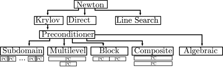
Fig. 1: Organization of a Newton-Krylov solver with potential points of customization. Although one can alter the type, parameters, or tolerances of Newton’s method, the Krylov solver, or the line search, we see that the majority of the potential customization and composition occurs at the level of the preconditioner. Possibilities include the use of algebraic preconditioners, such as direct solvers or sparse factorizations, or domain decomposition, multigrid, or composite solvers, which all have subcomponent solvers and preconditioners. These divisions may either be by subdomain, as with the additive Schwarz methods, or by physics field components, as with block preconditioners (for example, one block for pressures and one for velocities).

Nonlinear right-preconditioning of Newton’s method may take two forms. We describe our choice and comment on the alternative. At first glance, right-preconditioning of Newton’s method requires construction or application of the right-preconditioned Jacobian

$$\frac{\partial\mathbf{F}(\mathbf{M}(\mathbf{r},\mathbf{y}))}{\partial\mathbf{y}}=\mathbf{J}(\mathbf{M}(\mathbf{r},\mathbf{y}))\frac{\partial\mathbf{M}(\mathbf{r},\mathbf{y})}{\partial\mathbf{y}},$$ (4.3)

and we note that the computation of $\frac{\partial\mathbf{M}(\mathbf{r},\mathbf{y}_{i})}{\partial\mathbf{y}_{i}}$ is generally impractical. Consider the application of nonlinear right preconditioning on an iteration of Newton’s method, which would proceed in two steps:

$$\mathbf{y}_{i+1} =\mathbf{x}_{i}-\lambda\left(\frac{\partial\mathbf{M}(\mathbf{r},\mathbf{x}_{i})}{\partial\mathbf{x}_{i}}\right)^{-1}\mathbf{J}\left(\mathbf{M}(\mathbf{r},\mathbf{x}_{i})\right)^{-1}\mathbf{r}(\mathbf{M}(\mathbf{r},\mathbf{x}_{i}))$$

$$\mathbf{x}_{i+1} =\mathbf{M}(\mathbf{r},\mathbf{y}_{i+1}).$$

We may nest these two steps as

$$\mathbf{x}_{i+1}=\mathbf{M}(\mathbf{r},\mathbf{x}_{i}-\lambda\left(\frac{\partial\mathbf{M}(\mathbf{r},\mathbf{x}_{i})}{\partial\mathbf{x}_{i}}\right)^{-1}\mathbf{J}(\mathbf{M}(\mathbf{r},\mathbf{x}_{i}))^{-1}\mathbf{r}(\mathbf{M}(\mathbf{r},\mathbf{x}_{i}))),$$ (4.4)

and by Taylor expansion one may say that

$$\mathbf{M}(\mathbf{r},\mathbf{x}-\lambda\mathbf{d})=\mathbf{M}(\mathbf{r},\mathbf{x})-\lambda\left(\frac{\partial\mathbf{M}(\mathbf{r},\mathbf{x})}{\partial\mathbf{x}}\right)\mathbf{d}+...,$$

giving us the simplification

$$x_{i+1} \approx\mathbf{M}(\mathbf{r},\mathbf{x}_{i})-\lambda\left(\frac{\partial\mathbf{M}(\mathbf{r},\mathbf{x}_{i})}{\partial\mathbf{x}_{i}}\right)\left(\frac{\partial\mathbf{M}(\mathbf{r},\mathbf{x}_{i})}{\partial\mathbf{x}_{i}}\right)^{-1}\mathbf{J}(\mathbf{M}(\mathbf{r},\mathbf{x}_{i}))^{-1}\mathbf{r}(\mathbf{M}(\mathbf{r},\mathbf{x}_{i})))$$

$$=\mathbf{M}(\mathbf{r},\mathbf{x}_{i})-\lambda\mathbf{J}(\mathbf{M}(\mathbf{r},\mathbf{x}_{i}))^{-1}\mathbf{r}(\mathbf{M}(\mathbf{r},\mathbf{x}_{i}))$$

In this form, NEWT$\backslash$K$(\mathbf{F}(\mathbf{M}(\mathbf{r},\mathbf{x})),\mathbf{x})$ is easily implemented, as shown in Alg. 7.

Alg. 7 Right-Preconditioned Newton-Krylov Method

1:procedure NK($\mathbf{r}(\mathbf{M}(\mathbf{r},\mathbf{x})),\mathbf{x}_{i}$)

2:     $\phantom{\mathbf{x}_{i+1}}\mathllap{\mathbf{x}_{i+\frac{1}{2}}}=\mathbf{M}(\mathbf{r},\mathbf{x}_{i})$

3:     $\phantom{\mathbf{x}_{i+1}}\mathllap{\mathbf{d}}=\mathbf{J}(\mathbf{x}_{i+\frac{1}{2}})^{-1}\mathbf{r}(\mathbf{x}_{i+\frac{1}{2}})$

4:     $\mathbf{x}_{i+1}=\mathbf{x}_{i+\frac{1}{2}}+\lambda\mathbf{d}$ $\triangleright$ $\lambda$ determined by line search

5:return $\mathbf{x}_{i+1}$

Note that $\text{NEWT}\backslash\text{K}-_{R}\mathbf{M}$ is merely $\mathbf{M}*\text{NEWT}\backslash\text{K}$ in this form: one solver runs after the other. The connection between composition and preconditioning in Newton’s method provides an inkling of the advantages afforded to NEWT$\backslash$K as an inner composite solver combined with other methods. An alternative approach applies an approximation to (4.3) directly [4]. The approximation is

$$\mathbf{F}(\mathbf{M}(\mathbf{r},\mathbf{y}_{i})) =\mathbf{J}(\mathbf{M}(\mathbf{r},\mathbf{y}_{i}))\left(\frac{\partial\mathbf{M}(\mathbf{r},\mathbf{y}_{i})}{\partial\mathbf{y}_{i}}\right)(\mathbf{y}_{i+1}-\mathbf{y}_{i})$$

$$\approx\mathbf{J}(\mathbf{M}(\mathbf{r},\mathbf{y}_{i}))(\mathbf{M}(\mathbf{r},\mathbf{y}_{i}+[\mathbf{y}_{i+1}-\mathbf{y}_{i}])-\mathbf{x}_{i}),$$

which is solved for $\left[\mathbf{y}_{i+1}-\mathbf{y}_{i}\right]$. Right-preconditioning by the approximation requires an application of the nonlinear preconditioner for every inner Krylov iterate and limits our choices of Krylov solver to those tolerant of nonlinearity, such as flexible GMRES [57].

Alg. 8 Left-Preconditioned Newton-Krylov Method

1:procedure NEWT$\backslash$K($\mathbf{x}-\mathbf{M}(\mathbf{r},\mathbf{x}),\mathbf{x}_{i}$)

2:     $\phantom{\mathbf{x}_{i+1}}\mathllap{\mathbf{d}}=\frac{\partial(\mathbf{x}_{i}-\mathbf{M}(\mathbf{r},\mathbf{x}_{i}))}{\partial\mathbf{x}_{i}}^{-1}(\mathbf{x}_{i}-\mathbf{M}(\mathbf{r},\mathbf{x}_{i}))$ $\triangleright$ approximate inversion by Krylov method

3:     $\mathbf{x}_{i+1}=\mathbf{x}_{i}+\lambda\mathbf{d}$ $\triangleright$ $\lambda$ determined by line search

4:return $\mathbf{x}_{i+1}$

For nonlinear left-preconditioning, shown in Alg. 8, we replace the computation $\mathbf{r}(\mathbf{x}_{i})$ with $\mathbf{x}_{i}-\mathbf{M}(\mathbf{r},\mathbf{x}_{i})$ and take the Jacobian of the function as an approximation of

$$\frac{\partial(\mathbf{x}_{i}-\mathbf{M}(\mathbf{r},\mathbf{x}_{i}))}{\mathbf{x}_{i}}=\mathbf{I}-\frac{\partial\mathbf{M}(\mathbf{r},\mathbf{x}_{i})}{\partial\mathbf{x}_{i}},$$ (4.5)

where now the Jacobian is a linearization of $\mathbf{M}(\mathbf{r},\mathbf{x})$ and impractical to compute in most cases. In the particular case where the preconditioner is the nonlinear additive Schwarz method (NASM) (Section 5.2), this is known as ASPIN. In the case of NASM preconditioning, one has local block Jacobians, so the approximation of the preconditioned Jacobian as

$$\frac{\partial(\mathbf{x}-\mathbf{M}(\mathbf{r},\mathbf{x}))}{\partial\mathbf{x}}=\frac{\partial(\mathbf{x}-(\mathbf{x}-\sum_{b}\mathbf{J}^{b}(\mathbf{x}^{b})^{-1}\mathbf{r}^{b}(\mathbf{x}^{b})))}{\partial\mathbf{x}}\approx\sum_{b}\mathbf{J}^{b}(\mathbf{x}^{b*})^{-1}\mathbf{J}(\mathbf{x})$$ (4.6)

is used instead. The iteration requires only one inner nonlinear iteration and some small number of block solves, per outer nonlinear iteration. By contrast, direct differencing would require one inner iteration at each inner linear iteration for the purpose of repeated approximate Jacobian application. Note the similarity between ASPIN and the alternative form of right-preconditioning in terms of required components, with ASPIN being more convenient in the end.

4.5 Quasi-Newton (QN)

The class of methods for nonlinear systems of equations known as quasi-Newton methods [24] uses previous changes in residual and solution or other low-rank expansions [40] to form an approximation of the inverse Jacobian by a series of low rank updates. The approximate Jacobian inverse is then used to compute the search direction. If the update is done directly, it requires storing and updating the dense matrix $\mathbf{K}\approx\mathbf{J}^{-1}$, which is impractical for large systems. One may overcome this limitation by using limited-memory variants of the method [46, 51, 14, 49], which apply the approximate inverse Jacobian by a series of low-rank updates. The general form of QN methods is similar to that of NEWT$\backslash$K and is shown in Alg. 9.

Alg. 9 Quasi-Newton Update

1:procedure QN($\mathbf{r},\mathbf{x}_{i},\mathbf{s}_{i-1}\cdots\mathbf{s}_{i-m},\mathbf{y}_{i-1}\cdots\mathbf{y}_{i-m}$)

2:     $\mathbf{x}_{i+1}=\mathbf{x}_{i}-\lambda\mathbf{K}_{i}(\mathbf{K}_{0},\mathbf{s}_{i-1}...\mathbf{s}_{i-m},\mathbf{y}_{i-1}..\mathbf{y}_{i-m})\mathbf{r}(\mathbf{x}_{i})$ $\triangleright$ $\lambda$ determined by line search

3:     $\phantom{\mathbf{x}_{i+1}}\mathllap{\mathbf{s}_{i}}=\mathbf{x}_{i+1}-\mathbf{x}_{i}$

4:     $\phantom{\mathbf{x}_{i+1}}\mathllap{\mathbf{y}_{i}}=\mathbf{r}(\mathbf{x}_{i+1})-\mathbf{r}(\mathbf{x}_{i})$

5:return $\mathbf{x}_{i+1}$

A popular variant of the method, L-BFGS, can be applied efficiently by a two-loop recursion [51]:

Alg. 10 Two-Loop Recursion for L-BFGS

1:procedure $\mathbf{K}_{i}$($\mathbf{K}_{0},\mathbf{s}_{i-1}...\mathbf{s}_{i-m},\mathbf{y}_{i-1}...\mathbf{y}_{i-m},\mathbf{r}(\mathbf{x}_{i})$)

2:     $\mathbf{d}_{1}=\mathbf{r}(\mathbf{x}_{i})$

3:     for  $k=i-1$  do $i-m$

4:         $\alpha_{k}=\frac{\mathbf{s}_{k}^{\top}\mathbf{d}_{1}}{\mathbf{y}_{k}^{\top}\mathbf{s}_{k}}$

5:         $\mathbf{d}_{1}=\mathbf{d}_{1}-\alpha_{k}\mathbf{y}_{k}$

6:     end for

7:     $\mathbf{d}_{2}=\mathbf{K}_{0}\mathbf{d}_{1}$

8:     for  $k=i-m$  do $i-1$

9:         $\beta_{k}=\frac{\mathbf{y}_{k}^{\top}\mathbf{d}_{2}}{\mathbf{y}_{k}^{\top}\mathbf{s}_{k}}$

10:         $\mathbf{d}_{2}=\mathbf{d}_{2}+(\alpha_{k}-\beta_{k})\mathbf{s}_{k}$

11:     end for

12:return $\mathbf{d}_{2}$

Note that the update to the Jacobian in Alg. 10 is symmetric and shares many of the same limitations as nonlinear conjugate gradients (NCG) (Section 4.6). It may be perplexing, from an optimization perspective, to see L-BFGS and NCG applied to nonlinear PDEs as opposed to optimization problems. However, their exclusion from our discussion would be as glaring as leaving conjugate gradient methods out of a discussion of Krylov solvers for linear PDEs. In this paper we adhere to the limitations of NCG and QN and use them only for problems with symmetric Jacobians. In the case where L-BFGS is inapplicable, Broyden’s “good” and “bad” methods [13] have efficient limited memory constructions [14, 26, 29] and are recommended instead [52]. The overall performance of all these methods, however, may rival that of Newton’s method [38] in many cases. QN methods also have deep connections with Anderson mixing [28]. Anderson mixing, and the Broyden methods belong to a general class of Broyden-like methods [29].

The initial approximate inverse Jacobian $\mathbf{K}_{0}$ is often taken as the weighted [60] identity. However, one also can take $\mathbf{K}_{0}=\mathbf{J}_{0}^{-1}$ for lagged Jacobian $\mathbf{J}_{0}$. Such schemes greatly increase the robustness of lagged Newton’s methods when solving nonlinear PDEs [10]. Left-preconditioning for QN is trivial, and either the preconditioned or unpreconditioned residual may be used with the line search.

4.6 Nonlinear Conjugate Gradients

Nonlinear conjugate gradient methods [31] are a simple extension of the linear CG method but with the optimal step length in the conjugate direction determined by a line search rather than the exact formula that works in the linear case. NCG is outlined in Alg. 11. NCG requires storage of one additional vector for the conjugate direction $\mathbf{c}_{i}$ but has significantly faster convergence than does NRICH for many problems.

Alg. 11 Nonlinear CG

1:procedure NCG($\mathbf{r},\mathbf{x}_{i},\mathbf{c}_{i-1},\mathbf{r}_{i-1}$)

2:     $\phantom{\mathbf{x}_{i+1}}\mathllap{\mathbf{r}_{i}}=\mathbf{r}(\mathbf{x}_{i})$

3:     $\phantom{\mathbf{x}_{i+1}}\mathllap{\beta_{i}}=\frac{\mathbf{r}_{i}^{\top}(\mathbf{r}_{i}-\mathbf{r}_{i-1})}{\mathbf{r}_{i-1}^{\top}\mathbf{r}_{i-1}}$

4:     $\phantom{\mathbf{x}_{i+1}}\mathllap{\mathbf{c}_{i}}=-\mathbf{r}(\mathbf{x}_{i})+\beta_{i}\mathbf{c}_{i-1}$

5:     $\mathbf{x}_{i+1}=\mathbf{x}_{i}+\lambda\mathbf{c}_{i}$ $\triangleright$ $\lambda$ determined by line search

6:return $\mathbf{x}_{i+1}$

Several choices exist for constructing the parameter $\beta_{i}$ [21, 30, 31, 35]. We choose the Polak-Ribière-Polyak [53] variant. The application of nonlinear left-preconditioning is straightforward. Right-preconditioning is not conveniently applicable as is the case with QN in Section 4.5 and linear CG.

NCG has limited applicability because it suffers from the same issues as its linear cousin for problems with non-symmetric Jacobian. A common practice when solving nonlinear PDEs with NCG is to rephrase the problem in terms of the normal equations, which involves finding the root of $\mathbf{r}_{N}(\mathbf{x})=\mathbf{J}^{\top}\mathbf{r}(\mathbf{x})$. Since the Jacobian must be assembled and multiplied at every iteration, however, the normal equation solver is not a reasonable algorithmic choice, even with drastic lagging of Jacobian assembly. The normal equations also have a much worse condition number than does the original PDE. In our experiments, we use the conjugacy-ensuring CP line search.

5 Decomposition Solvers

An extremely important class of methods for linear problems is based on domain or hierarchical decomposition, and so we consider nonlinear variants of domain decomposition and multilevel algorithms. We introduce three different nonlinear solver algorithms based on point-block solves, local subdomain solves, and coarse-grid solves.

These methods require a trade-off between the amount of computation dedicated to solving local or coarse problems and the communication for global assembly and convergence monitoring. Undersolving the subproblems wastes the communication overhead of the outer iteration, and oversolving exacerbates issues of load imbalance and quickly has diminishing returns with respect to convergence. The solvers in this section exhibit a variety of features related to these trade-offs.

The decomposition solvers do not guarantee convergence. While they might converge, the obvious extension is to use them in conjunction with the global solvers as nonlinear preconditioners or accelerators. As the decomposition solvers expose more possibilities for parallelism or acceleration, their effective use in the nonlinear context should provide similar benefits to the analogous solvers in the linear context. A major disadvantage of these solvers is that each of them requires additional information about the local problems, a decomposition, or hierarchy of discretizations of the domain.

5.1 Gauss-Seidel-Newton (GSN)

Effective methods may be constructed by exact solves on subproblems. Suppose that the problem easily decomposes into $n_{b}$ small block subproblems. If Newton’s method is applied multiplicatively by blocks, the resulting algorithm is known as Gauss-Seidel-Newton and is shown in Alg. 12. Similar methods are commonly used as nonlinear smoothers [33, 34]. To construct GSN, we define the individual block Jacobians $\mathbf{J}^{b}(\mathbf{x}^{b})$ and residuals $\mathbf{r}^{b}(\mathbf{x}^{b})$; $\mathbf{R}^{b}$, which restricts to a block; and $\mathbf{P}^{b}$, which injects the solution to that block back into the overall solution. The point-block solver runs until the norm of the block residual is less than $\epsilon^{b}$ or $m_{b}$ steps have been taken.

Alg. 12 Gauss-Seidel-Newton

1:procedure GSN($\mathbf{r},\mathbf{x}_{i}$)

2:     $\mathbf{x}_{i+1}=\mathbf{x}_{i}$

3:     for  $b=1$  do $n_{b}$

4:         $\mathbf{x}^{b}_{i,0}=\mathbf{R}^{b}\mathbf{x}_{i+1}$

5:         while  $\|\mathbf{r}^{b}\|_{2}>\epsilon^{b}$ and $j<m_{b}$  do

6:              $\phantom{\mathbf{x}_{i,j}^{b}}\mathllap{j}=j+1$

7:              $\mathbf{x}_{i,j}^{b}=\mathbf{x}_{i,j-1}^{b}-\mathbf{J}^{b}(\mathbf{x}_{i,j-1}^{b})^{-1}\mathbf{r}_{i,j-1}^{b}$ $\triangleright$ direct inversion of block Jacobian

8:              $\mathbf{r}_{i,j}^{b}=\mathbf{r}^{b}(\mathbf{x}^{b}_{i,j})$

9:         end while

10:         $\mathbf{x}_{i+1}=\mathbf{x}_{i+1}-\mathbf{P}^{b}(\mathbf{x}_{i,0}^{b}-\mathbf{x}_{i,j}^{b})$

11:     end for

12:return $\mathbf{x}_{i+1}$

GSN solves small subproblems with a fair amount of computational work per degree of freedom and thus has high arithmetic intensity. It is typically greater than two times the work per degree of freedom of NRICH for scalar problems, and even more for vector problems where the local Newton solve is over several local degrees of freedom.

When used as a solver, GSN requires one reduction per iteration. However, stationary solvers, in both the linear and nonlinear case, do not converge robustly for large problems. Accordingly, GSN would typically be used as a preconditioner, making monitoring of global convergence, within the GSN iterations, unnecessary. Thus, in practice there is no synchronization; GSN is most easily implemented with multiplicative update on serial subproblems and additively in parallel.

5.2 Nonlinear Additive Schwarz Method

GSN can be an efficient underlying kernel for sequential nonlinear solvers. For parallel computing, however, an additive method with overlapping subproblems has desirable properties with respect to communication and arithmetic intensity. The nonlinear additive Schwarz methods allow for medium-sized subproblems to be solved with a general method, and the corrections from that method summed into a global search direction. Here we limit ourselves to decomposition by subdomain rather than splitting the problem into fields. While eliminating fields might be tempting, the construction of effective methods of this sort is significantly more involved than in the linear case, and many interesting problems do not have such a decomposition readily available. Using subdomain problems $\mathbf{F}^{B}$, restrictions $\mathbf{R}^{B}$, injections $\mathbf{P}^{B}$, and solvers $\mathbf{M}^{B}$, Alg. 13 outlines the NASM solver with $n_{B}$ subdomains.

Alg. 13 Nonlinear Additive Schwarz

1:procedure NASM($\mathbf{r},\mathbf{x}_{i}$)

2:     for  $B=1$  do $n_{B}$

3:         $\mathbf{x}^{B}_{0}=\mathbf{R}^{B}\mathbf{x}_{i}$

4:         $\phantom{\mathbf{x}^{B}_{0}}\mathllap{\mathbf{x}^{B}}=\mathbf{M}^{B}(\mathbf{r}^{B},\mathbf{x}^{B}_{0})$

5:         $\phantom{\mathbf{x}^{B}_{0}}\mathllap{\mathbf{y}^{B}}=\mathbf{x}^{B}_{0}-\mathbf{x}^{B}$

6:     end for

7:     $\mathbf{x}_{i+1}=\mathbf{x}_{i}-\displaystyle\sum_{B=1}^{n_{B}}\mathbf{P}^{B}\mathbf{y}^{B}$

8:return $\mathbf{x}_{i+1}$

Two choices exist for the injections $\mathbf{P}^{B}$ in the overlapping regions. We will use NASM to denote the variant that uses overlapping injection corresponding to the whole subproblem step. The second variant, restricted additive Schwarz (RAS), injects the step in a non-overlapping fashion. The subdomain solvers are typically Newton-Krylov, but the other methods described in this paper are also applicable.

5.3 Full Approximation Scheme

FAS [6] accelerates convergence by advancing the nonlinear solution on a series of coarse rediscretizations of the problem. As with standard linear multigrid, the cycle may be constructed either additively or multiplicatively, with multiplicative being more effective in terms of per-iteration convergence. Additive approaches provide the usual advantage of allowing the coarse-grid corrections to be computed in parallel. We do not consider additive FAS in this paper.

Given the smoother $\mathbf{M}_{s}(\mathbf{r},\mathbf{x})$ at each level, as well as restriction ($\mathbf{R}$), prolongation ($\mathbf{P}$) and injection ($\mathbf{\hat{R}}$) operators, and the coarse nonlinear function $\mathbf{F}^{H}$, the FAS V-cycle takes the form shown in Alg. 14.

Alg. 14 Full Approximation Scheme

1:procedure FAS($\mathbf{r},\mathbf{x}_{i}$)

2:     $\phantom{\mathbf{x}_{i+1}}\mathllap{\mathbf{x}_{s}}=\mathbf{M}_{s}(\mathbf{r},\mathbf{x}_{i})$

3:     $\phantom{\mathbf{x}_{i+1}}\mathllap{\mathbf{x}^{H}_{i}}=\mathbf{\hat{R}}\mathbf{x}_{s}$

4:     $\phantom{\mathbf{x}_{i+1}}\mathllap{\mathbf{b}^{H}}=\mathbf{R}[\mathbf{b}-\mathbf{F}(\mathbf{x}_{s})]+\mathbf{F}^{H}(\mathbf{x}^{H}_{i})$

5:     $\phantom{\mathbf{x}_{i+1}}\mathllap{\mathbf{x}_{c}}=\mathbf{x}_{s}+\mathbf{P}[\text{FAS}(\mathbf{F}^{H}-\mathbf{b}^{H},\mathbf{x}^{H}_{i})-\mathbf{x}^{H}_{i}]$

6:     $\phantom{\mathbf{x}_{i+1}}\mathllap{\mathbf{x}_{i+1}}=\mathbf{M}_{s}(\mathbf{r},\mathbf{x}_{c})$

7:return $\mathbf{x}_{i+1}$

The difference between FAS and linear multigrid is the construction of the coarse RHS $\mathbf{b}^{H}$. In FAS  it is guaranteed that if an exact solution $\mathbf{x}^{*}$ to the fine problem is found,

$$\text{FAS}(\mathbf{r}^{H}-\mathbf{b}^{H},\mathbf{\hat{R}}\mathbf{x}^{*})-\mathbf{\hat{R}}\mathbf{x}^{*}=0.$$ (5.1)

The correction is not necessary in the case of linear multigrid. However, FAS is mathematically identical to standard multigrid when applied to a linear problem.

The stellar algorithmic performance of linear multigrid methods is well documented, but the arithmetic intensity may be low. FAS presents an interesting alternative to $\text{NEWT}\backslash\text{K}-\text{MG}$, since it may be configured with high arithmetic intensity operations at all levels. The smoothers are themselves nonlinear solution methods. FAS-type methods are applicable to optimization problems as well as nonlinear PDEs [8], with optimization methods used as smoothers [50].

5.4 Summary

We have now introduced the mathematical construction of nonlinear composed solvers. We have also described two classes of nonlinear solvers, based on solving either the global problem or some partition of it. The next step is to describe a set of test problems with different limitations with respect to which methods will work for them, construct a series of instructive example solvers using composition of the previously defined solvers, and test them. We have made an effort to create flexible and robust software for composed nonlinear solvers. The organization of the software is in the spirit of PETSc and includes several interchangeable component solvers, including NEWT$\backslash$K; iterative solvers such as ANDERSON and QN that may contain an inner preconditioner; decomposition solvers such as NASM and FAS, which are built out of subdomain solvers; and metasolvers implementing compositions . A diagram enumerating the composed solver framework analogous to that of the preconditioned NEWT$\backslash$K case is shown in Fig. 2.

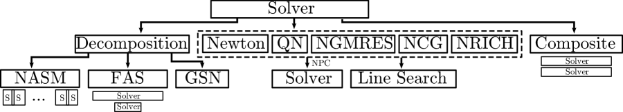
Fig. 2: Organization of the components of a composed nonlinear solver. We discard the difference between solvers and preconditioners and see that the nesting and potential for recursive customization lives at every level of the tree. Possibilities include iterative solvers (including Newton’s method) with nonlinear preconditioning, composite solvers consisting of several subsolvers, or decomposition solvers consisting of subdomain or coarse nonlinear solvers.

6 Experiments

We will demonstrate the efficacy nonlinear composition and preconditioning by experiments with a suite of nonlinear partial differential equations that show interesting behavior in regimes with difficult nonlinearities. These problems are nonlinear elasticity, the lid-driven cavity with buoyancy, and the $p$-Laplacian.

One goal of this paper is to be instructive. We first try to solve the problem efficiently with the standard solvers, then choose a subset of the above solvers for each problem and show how to gain advantage by using composition methods. Limitations of discretization or problem regime are noted, and we discuss how the solvers may be used under these limitations. We also explain how readers may run the examples in this paper and experiment with the solvers both on the test examples shown here and on their own problems. We feel we have no “skin in the game” and are not trying to show that some approaches are better or worse than others.

6.1 Methods

Our set of test algorithms is defined by the preconditioning of an iterative solver with a decomposition solver, or the composition of two solvers with different advantages. In the case of the decomposition solvers, we choose one or two configurations per test problem, in order to avoid the combinatorial explosion of potential methods that already is apparent from the two forms of composition combined with the multitude of methods.

Our primary measure of performance is time to solution, which is both problem and equipment dependent. Since it depends strongly on the relative cost of function evaluation, Jacobian assembly, matrix multiplication, and subproblem or coarse solve, we also record number of nonlinear iterations, linear iterations, linear preconditioner applications, function evaluations, Jacobian evaluations, and nonlinear preconditioner applications. These measures allow us to characterize efficiency disparities in terms of major units of computational work.

We make a good faith effort to tune each method for performance while keeping subsolver parameters invariant. Occasionally, we err on the side of oversolving for the inner solvers, to make the apples-to-apples comparison more consistent between closely related methods. The results here should be taken as a rough guide to improving solver performance and robustness. The test machine is a 64-core AMD Opteron 6274-based [1] machine with 128 GB of memory. The problems are run with one MPI process per core. Plots of convergence are generated with Matplotlib [36], and plots of solutions are generated with Mayavi [56].

6.2 Nonlinear Elasticity

A Galerkin formulation for nonlinear elasticity may be stated as

$$\int_{\Omega}F\cdot S:\nabla v\,d\Omega+\int_{\Omega}b\cdot v\,d\Omega=0$$ (6.1)

for all test functions $v\in\mathcal{V}$; $F=\nabla\mathbf{u}+I$ is the deformation gradient. We use the Saint Venant-Kirchhoff model of hyperelasticity with second Piola-Kirchhoff stress tensor $S=\lambda\mathrm{tr}(E)I+2\mu E$ for Lagrangian Green strain $E=F^{\top}F-I$ and Lamé parameters $\lambda$ and $\mu$, which may be derived from a given Young’s modulus and Poisson ratio. We solve for displacements $\mathbf{u}\in\mathcal{V}$, given a constant load vector $b$ imposed on the structure.

The domain $\Omega$ is a $60^{\circ}$ cylindrical arch of inner radius $100$ m. Homogeneous Dirichlet boundary conditions are imposed on the outer edge of the ends of the arch. The goal is to “snap through” the arch, causing it to sag under the load rather than merely compressing it. To cause the sag, we set $b=-\mathbf{e}_{y}$ and set the Lamé constants consistent with a Young’s modulus of 100 and a Poisson ratio of 0.2. The nonlinearity is highly activated during the process of snapping through and may be tuned to present a great deal of difficulty to traditional nonlinear solvers. The problem is discretized by using hexahedral $\mathbf{Q}_{1}$ finite elements on a logically structured grid, deformed to form the arch. The grid is 401x9x9, and therefore the problem has 97,443 degrees of freedom. The problem is a three-dimensional extension of a problem put forth by Wriggers [75]. The unstressed and converged solutions are shown in Fig. 3.

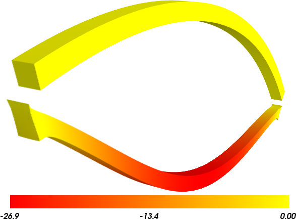
Fig. 3: Unstressed and stressed configurations for the elasticity test problem. Coloration indicates vertical displacement in meters.

For 3D hexahedral FEM discretizations, GSN and related algorithms are inefficient because for each degree of freedom each element in the support of the degree of freedom must be visited, resulting in eight visits to an interior element per sweep. Instead, we focus on algorithms requiring only a single visit to each cell, restricting us to function and Jacobian evaluations. Such approaches are also available in the general unstructured FEM case, and these experiments may guide users in regimes where no decomposition solvers are available.

For the experiments, we emphasize the role that nonlinear composition and series acceleration may play in the acceleration of nonlinear solvers. The problem is amenable to NCG, ANDERSON, and NEWT$\backslash$K with an algebraic multigrid preconditioner. We test a number of combinations of these solvers. Even though we have a logically structured grid, we approach the problem as if no reasonable grid hierarchy or domain decomposition were available. The solver combinations we use are listed in Table 2. In all the following tables, Solver denotes outer solver, LPC denotes the linear PC when applicable, NPC denotes the nonlinear PC when applicable, Side denotes the type of preconditioning, Smooth denotes the level smoothers used in the multilevel method (MG/FAS), and LS denotes line search.

Table 2: Series of solvers for the nonlinear elasticity test problem.

Name	Solver	LPC	NPC	Side	Smooth	LS
NCG	NCG					CP
$\text{NEWT}\backslash\text{K}-\text{MG}$	NEWT$\backslash$K	MG	–	–	SOR	BT
$\text{NCG}-_{L}(\text{NEWT}\backslash\text{K}-\text{MG})$	NCG	–	$\text{NEWT}\backslash\text{K}-\text{MG}$	L	SOR	CP
$\text{NGMRES}-_{R}(\text{NEWT}\backslash\text{K}-\text{MG})$	NGMRES	–	$\text{NEWT}\backslash\text{K}-\text{MG}$	R	SOR	CP
$\text{NCG}(10)+(\text{NEWT}\backslash\text{K}-\text{MG})$	NCG,NEWT$\backslash$K	MG	–	–	SOR	CP/BT
$\text{NCG}(10)*(\text{NEWT}\backslash\text{K}-\text{MG})$	NCG,NEWT$\backslash$K	MG	–	–	SOR	CP/BT

For the NEWT$\backslash$K methods, we precondition the inner GMRES solve with a smoothed aggregation algebraic multigrid method provided by the GAMG package in PETSc. The relative tolerance for the GMRES solve is $10^{-3}$. For all instances of the NCG solver, the CP line search initial guess for $\lambda$ is the final value from the previous nonlinear iteration. In the case of $\text{NGMRES}-_{R}(\text{NEWT}\backslash\text{K}-\text{MG})$ the inner line search is L2. NGMRES stores up to 30 previous solutions and residuals for all experiments. The outer line search for $\text{NCG}-_{L}(\text{NEWT}\backslash\text{K}-\text{MG})$ is a second-order secant approximation rather than first-order as depicted in Alg. 1. For the composite examples, 10 iterations of NCG are used as one of the subsolvers, denoted $\text{NCG}(10)$. The additive composition ’s weights are determined by the ANDERSON minimization mechanism as described in Section 4.3.

The example, SNES ex16.c, can be run directly by using a default PETSc installation. The command line used for these experiments is

./ex16 -da_grid_x 401 -da_grid_y 9 -da_grid_z 9 -height 3 -width 3
  -rad 100 -young 100 -poisson 0.2 -loading -1 -ploading 0

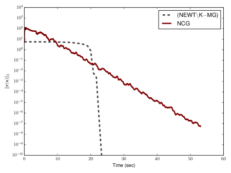
Fig. 4: $(\text{NEWT}\backslash\text{K}-\text{MG})$ and NCG convergence.

Table 3: $(\text{NEWT}\backslash\text{K}-\text{MG})$ and NCG results.

Solver	T	N. It	L. It	Func	Jac	PC	NPC
$(\text{NEWT}\backslash\text{K}-\text{MG})$	23.43	27	1556	91	27	1618	–
NCG	53.05	4495	0	8991	–	–	–

The solvers shown in Table 3 converge slowly. $\text{NEWT}\backslash\text{K}-\text{MG}$ takes 27 nonlinear iterations and 1,618 multigrid V-cycles to reach convergence. NCG requires 8,991 function evaluations and since it is unpreconditioned, scales unacceptably with problem size with respect to number of iterations. Note in Fig. 4 that while NCG takes an initial jump and then decreases at a constant rate, $\text{NEWT}\backslash\text{K}-\text{MG}$ is near stagnation until the end, when it suddenly drops into the basin of attraction.

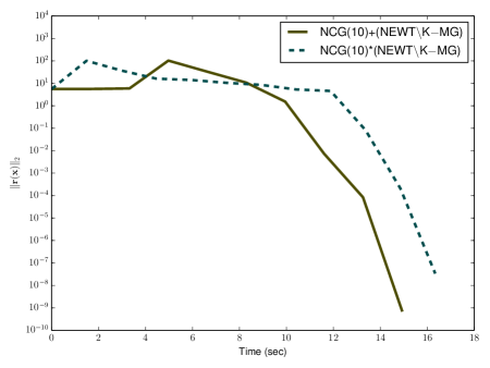
Fig. 5: $\text{NCG}(10)+(\text{NEWT}\backslash\text{K}-\text{MG})$ and $\text{NCG}(10)*(\text{NEWT}\backslash\text{K}-\text{MG})$ convergence.

Table 4: $\text{NCG}(10)+(\text{NEWT}\backslash\text{K}-\text{MG})$ and $\text{NCG}(10)*(\text{NEWT}\backslash\text{K}-\text{MG})$ results.

Solver	T	N. It	L. It	Func	Jac	PC	NPC
$\text{NCG}(10)+(\text{NEWT}\backslash\text{K}-\text{MG})$	14.92	9	459	218	9	479	–
$\text{NCG}(10)*(\text{NEWT}\backslash\text{K}-\text{MG})$	16.34	11	458	251	11	477	–

Results for composition are listed in Table 4. Additive and multiplicative composite combination provides roughly similar speedups for the problem, with more total outer iterations in the additive case. As shown in Fig. 5, neither the additive nor multiplicative methods stagnate. After the same initial jump and convergence at the pace of NCG, the basin of attraction is reached, and the entire iteration converges quadratically as should be expected with NEWT$\backslash$K.

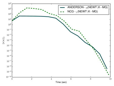
Fig. 6: $\text{NGMRES}-_{R}(\text{NEWT}\backslash\text{K}-\text{MG})$ and $\text{NCG}-_{L}(\text{NEWT}\backslash\text{K}-\text{MG})$ convergence.

Table 5: $\text{NGMRES}-_{R}(\text{NEWT}\backslash\text{K}-\text{MG})$ and $\text{NCG}-_{L}(\text{NEWT}\backslash\text{K}-\text{MG})$ results.

Solver	T	N. It	L. It	Func	Jac	PC	NPC
$\text{NGMRES}-_{R}(\text{NEWT}\backslash\text{K}-\text{MG})$	9.65	13	523	53	13	548	13
$\text{NCG}-_{L}(\text{NEWT}\backslash\text{K}-\text{MG})$	9.84	13	529	53	13	554	13

Left-preconditioning of NCG and ANDERSON with NEWT$\backslash$K$-$MG provides even greater benefits, as shown in Fig. 6 and Table 5. The number of iterations is nearly halved from the unpreconditioned case, and the number of linear preconditioner applications is only slightly increased compared with the composition cases. In Fig. 6, we see that the Newton’s method-preconditioned nonlinear Krylov solvers never dive as NEWT$\backslash$K did but maintain rapid, mostly constant convergence instead. This constant convergence is a significantly more efficient path to solution than the $\text{NEWT}\backslash\text{K}-\text{MG}$ solver alone.

6.3 Driven Cavity

The driven cavity formulation used for the next set of experiments can be stated as

$$-\Delta\mathbf{u}-\nabla\times\Omega = 0$$ (6.2)

$$-\Delta\Omega+\nabla\cdot(\mathbf{u}\Omega)-\mathrm{Gr}\nabla_{x}T = 0$$ (6.3)

$$-\Delta T+\mathrm{Pr}\nabla\cdot\mathbf{u} = 0.$$ (6.4)

The fluid motion is driven in part by a moving lid and in part by buoyancy. A Grashof number $Gr=2e4$, Prandtl number $Pr=1$, and lid velocity of 100 are used in these experiments. No-slip, rigid-wall Dirichlet conditions are imposed for $\mathbf{u}$. Dirichlet conditions are used for $\Omega$, based on the definition of vorticity, $\Omega=\nabla\times\mathbf{u}$, where along each constant coordinate boundary the tangential derivative is zero. Dirichlet conditions are used for $T$ on the left and right walls, and insulating homogeneous Neumann conditions are used on the top and bottom walls. A finite-difference approximation with the usual 5-point stencil is used to discretize the boundary value problem in order to obtain a nonlinear system of equations. Upwinding is used for the divergence (convective) terms and central differencing for the gradient (source) terms.

In these experiments, we emphasize the use of ANDERSON, MG or FAS, and GSN. The solver combinations are listed in Table 6. The multilevel methods use a simple series of structured grids, with the smallest being 5x5 and the largest being 257x257. With four fields per grid point, we have an overall system size of 264,196 unknowns. In $\text{NEWT}\backslash\text{K}-\text{MG}$, the Jacobian is rediscretized on each level. GSN is used as the smoother for FAS and solves the four-component block problem corresponding to (6.2) per grid point in a simple sweep through the processor local part of the domain.

The example, SNES ex19.c, can be run directly by using a default PETSc installation. The command line used for these experiments is

  ./ex19 -da_refine 6 -da_grid_x 5 -da_grid_y 5 -grashof 2e4 -lidvelocity 100 -prandtl 1.0

and the converged solution using these options is shown in Fig. 7.

Table 6: Solvers for the lid driven cavity problem.

Name	Solver	LPC	NPC	Side	MG/FASSmooth.	LS
$(\text{NEWT}\backslash\text{K}-\text{MG})$	NEWT$\backslash$K	MG	–	–	SOR	BT
$\text{NGMRES}-_{R}(\text{NEWT}\backslash\text{K}-\text{MG}$)	NGMRES	MG	NEWT$\backslash$K	R	SOR	–
FAS	FAS	–	–	–	GSN	–
$\text{NRICH}-_{L}\text{FAS}$	NRICH	–	FAS	L	GSN	L2
$\text{NGMRES}-_{R}\text{FAS}$	NGMRES	–	FAS	R	GSN	–
$\text{FAS}*(\text{NEWT}\backslash\text{K}-\text{MG})$	FAS/NEWT$\backslash$K	MG	–	–	SOR/GSN	BT
$\text{FAS}+(\text{NEWT}\backslash\text{K}-\text{MG})$	FAS/NEWT$\backslash$K	MG	–	–	SOR/GSN	BT

All linearized problems in the NEWT$\backslash$K iteration are solved by using GMRES with geometric multigrid preconditioning to a relative tolerance of $10^{-8}$. There are five levels, with Chebychev$-$SOR smoothers on each level. For FAS, the smoother is GSN(5). The coarse-level smoother is five iterations of NEWT$\backslash$K-LU; chosen for robustness. In the case of $\text{NGMRES}-_{R}(\text{NEWT}\backslash\text{K}-\text{MG})$ and $\text{FAS}+(\text{NEWT}\backslash\text{K}-\text{MG})$, the $\text{NEWT}\backslash\text{K}-\text{MG}$ step is damped by one half. Note that acting alone, this damping would cut the rate of convergence to linear with a rate constant $\frac{1}{2}$. The ideal step size is recovered by the minimization procedure. $\text{NEWT}\backslash\text{K}-\text{MG}$ is undamped in all other tests.

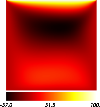
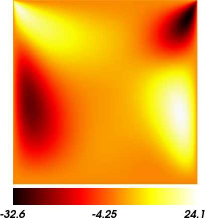
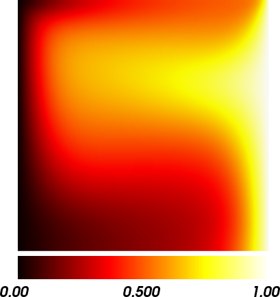
Fig. 7: $\mathbf{u}_{x}$, $\mathbf{u}_{y}$, and temperature profiles for the lid driven cavity solution.

In these experiments we emphasize the total number of V-cycles, linear and nonlinear, since they dominate the runtime and contain the lion’s share of the communication and floating-point operations.

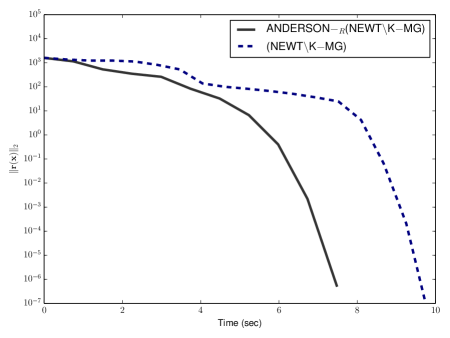
Fig. 8: $\text{NGMRES}-_{R}(\text{NEWT}\backslash\text{K}-\text{MG})$ and $(\text{NEWT}\backslash\text{K}-\text{MG})$ convergence.

Table 7: $\text{NGMRES}-_{R}(\text{NEWT}\backslash\text{K}-\text{MG})$ and $(\text{NEWT}\backslash\text{K}-\text{MG})$ results.

Solver	T	N. It	L. It	Func	Jac	PC	NPC
$\text{NGMRES}-_{R}(\text{NEWT}\backslash\text{K}-\text{MG})$	7.48	10	220	21	50	231	10
$(\text{NEWT}\backslash\text{K}-\text{MG})$	9.83	17	352	34	85	370	–

In Table 7, we see that Newton’s method converges in 17 iterations, with 370 V-cycles. Using NGMRES instead of a line search provides some benefit, as $\text{NGMRES}-(\text{NEWT}\backslash\text{K}-\text{MG})$ takes 231 V-cycles and 10 iterations.

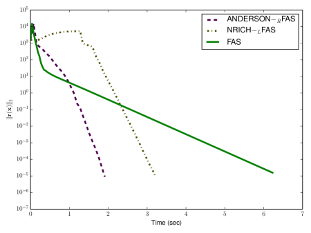
Fig. 9: $\text{NGMRES}-_{R}\text{FAS}$, $\text{NRICH}-_{L}\text{FAS}$, and FAS convergence.

Table 8: $\text{NGMRES}-_{R}\text{FAS}$, $\text{NRICH}-_{L}\text{FAS}$, and FAS results.

Solver	T	N. It	L. It	Func	Jac	PC	NPC
$\text{NGMRES}-_{R}\text{FAS}$	1.91	24	0	447	83	166	24
$\text{NRICH}-_{L}\text{FAS}$	3.20	50	0	1180	192	384	50
FAS	6.23	162	0	2382	377	754	–

$\text{NRICH}-_{L}\text{FAS}$ takes 50 V-cycles, at the expense of three more fine-level function evaluations per iteration. $\text{NGMRES}-_{R}\text{FAS}$ reduces the number of V-cycles to 24 at the expense of more communication.

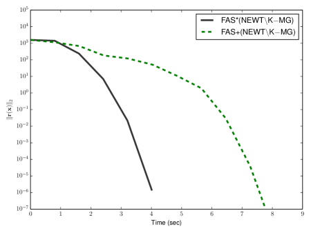
Fig. 10: $\text{FAS}*(\text{NEWT}\backslash\text{K}-\text{MG})$ and $\text{FAS}+(\text{NEWT}\backslash\text{K}-\text{MG})$ convergence.

Table 9: $\text{FAS}*(\text{NEWT}\backslash\text{K}-\text{MG})$ and $\text{FAS}+(\text{NEWT}\backslash\text{K}-\text{MG})$ results.

Solver	T	N. It	L. It	Func	Jac	PC	NPC
$\text{FAS}*(\text{NEWT}\backslash\text{K}-\text{MG})$	4.01	5	80	103	45	125	–
$\text{FAS}+(\text{NEWT}\backslash\text{K}-\text{MG})$	8.07	10	197	232	90	288	–

Composed nonlinear methods are shown in Table 9. Multiplicative composition consisting of FAS and NEWT$\backslash$K$-$MG reduces the total number of V-cycles to 130. Additive composition using the least-squares minimization is less effective, taking 298 V-cycles. Note in Fig. 10 that both the additive and multiplicative solvers show that combining FAS and NEWT$\backslash$K-MG may speed solution, with multiplicative combination being significantly more effective.

6.4 Tuning the Solvers to Obtain Convergence

We now show how the composed and preconditioned solves may be tuned for more difficult nonlinearities where the basic methods fail to converge using the same model problem. For Grashof number $\mathrm{Gr}<10^{4}$ and Prandtl number $\mathrm{Pr}=1.0$, Newton’s method converges well:

lid velocity = 100, prandtl # = 1, grashof # = 10000
  0 SNES Function norm 715.271
  1 SNES Function norm 623.41
  2 SNES Function norm 510.225
   ⋮
  6 SNES Function norm 0.269179
  7 SNES Function norm 0.00110921
  8 SNES Function norm 1.12763e-09
Nonlinear solve converged due to CONVERGED_FNORM_RELATIVE iterations 8
Number of SNES iterations = 8

For higher Grashof number, Newton’s method stagnates

./ex19 -lidvelocity 100 -grashof 5e4 -da_refine 4 -pc_type lu -snes_monitor_short -snes_converged_reason
lid velocity = 100, prandtl # = 1, grashof # = 50000
  0 SNES Function norm 1228.95
  1 SNES Function norm 1132.29
            ⋮
 29 SNES Function norm 580.937
 30 SNES Function norm 580.899

It also fails with the standard continuation strategy from coarser meshes (not shown). We next try nonlinear multigrid, in the hope that multiple updates from a coarse solution are sufficient, using GS as the nonlinear smoother,

./ex19 -lidvelocity 100 -grashof 5e4 -da_refine 4 -snes_monitor_short -snes_converged_reason -snes_type fas
       -fas_levels_snes_type ngs -fas_levels_snes_max_it 6 -snes_max_it 25
lid velocity = 100, prandtl # = 1, grashof # = 50000
  0 SNES Function norm 1228.95
  1 SNES Function norm 574.793
  2 SNES Function norm 513.02
  3 SNES Function norm 216.721
  4 SNES Function norm 85.949
  5 SNES Function norm 108.24
  6 SNES Function norm 207.469
  ⋮
 22 SNES Function norm 131.866
 23 SNES Function norm 114.817
 24 SNES Function norm 71.4699
 25 SNES Function norm 63.5413

But the residual norm just jumps around and the method does not converge. We then accelerate the method with ANDERSON and obtain convergence.

./ex19 -lidvelocity 100 -grashof 5e4 -da_refine 4 -snes_monitor_short -snes_converged_reason -snes_type anderson
       -npc_snes_max_it 1 -npc_snes_type fas  -npc_fas_levels_snes_type ngs -npc_fas_levels_snes_max_it 6
lid velocity = 100, prandtl # = 1, grashof # = 50000
  0 SNES Function norm 1228.95
  1 SNES Function norm 574.793
  2 SNES Function norm 345.592
  3 SNES Function norm 155.476
  4 SNES Function norm 70.2302
  5 SNES Function norm 40.3618
  6 SNES Function norm 29.3065
  7 SNES Function norm 14.2497
  8 SNES Function norm 4.80462
  9 SNES Function norm 4.15985
 10 SNES Function norm 2.13428
 11 SNES Function norm 1.57717
 12 SNES Function norm 0.60919
 13 SNES Function norm 0.150496
 14 SNES Function norm 0.0355709
 15 SNES Function norm 0.00705481
 16 SNES Function norm 0.00164509
 17 SNES Function norm 0.000464835
 18 SNES Function norm 6.02035e-05
 19 SNES Function norm 1.11713e-05
Nonlinear solve converged due to CONVERGED_FNORM_RELATIVE iterations 19
Number of SNES iterations = 19

We can restore the convergence to a few iterates by increasing the power of the nonlinear smoothers in FASẆe replace GSN by six iterations of Newton using the default linear solver of GMRES plus ILU(0). Note that as a solver alone this does not converge but it performs very well as a smoother for FAS.

./ex19 -lidvelocity 100 -grashof 5e4 -da_refine 4 -snes_monitor_short -snes_converged_reason -snes_type anderson
       -npc_snes_max_it 1 -npc_snes_type fas -npc_fas_levels_snes_type newtonls -npc_fas_levels_snes_max_it 6
       -npc_fas_levels_snes_linesearch_type basic -npc_fas_levels_snes_max_linear_solve_fail 30
       -npc_fas_levels_ksp_max_it 20
lid velocity = 100, prandtl # = 1, grashof # = 50000
  0 SNES Function norm 1228.95
  1 SNES Function norm 0.187669
  2 SNES Function norm 0.0319743
  3 SNES Function norm 0.00386815
  4 SNES Function norm 2.24093e-05
  5 SNES Function norm 5.38246e-08
Nonlinear solve converged due to CONVERGED_FNORM_RELATIVE iterations 5
Number of SNES iterations = 5

Thus we have demonstrated how one may experimentally add composed solvers to go from complete lack of convergence to convergence with a small number of iterations.

6.5 $p$-Laplacian

The regularized $p$-Laplacian formulation used for these experiments is

$$-\nabla\cdot((\epsilon^{2}+\frac{1}{2}|\nabla u|^{2})^{(p-2)/2}\nabla u)=c,$$

where $\epsilon=10^{-5}$ is the regularization parameter and $p$ the exponent of the Laplacian. When $p=2$ the $p$-Laplacian reduces to the Poisson equation. We consider the case where $p=5$ and $c=0.1$. The domain is $[-1,1]\times[-1,1]$ and the initial guess is $u_{0}(x,y)=xy(1-x^{2})(1-y^{2})$. The grid used is 385x385, leading to a total of 148,225 unknowns in the system. The initial and converged solutions are shown in Fig. 11.

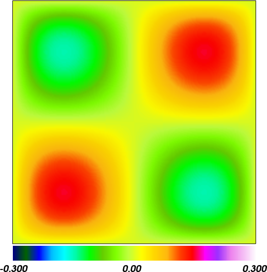
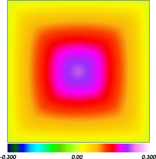
Fig. 11: Initial and converged solutions to the $p=5$ $p$-Laplacian.

The example, SNES ex15.c, can be run directly by using a default PETSc installation. The command line used for these experiments is

./ex15 -da_refine 7 -da_overlap 6 -p 5.0 -lambda 0.0 -source 0.1

Table 10: Solvers for the $p$-Laplacian problem. SubPC denotes the linear solver at the block level.

Name	Solver	LPC	NPC	Side	SubPC	LS
$\text{NEWT}\backslash\text{K}-\text{ASM}$	NEWT$\backslash$K	ASM	–	–	LU	BT
QN	QN	–	–	–		CP
RAS	RAS	–	–	–	LU	CP
$\text{RAS}+(\text{NEWT}\backslash\text{K}-\text{ASM})$	RAS/NEWT$\backslash$K	ASM	–	–	LU	BT
$\text{RAS}*(\text{NEWT}\backslash\text{K}-\text{ASM})$	RAS/NEWT$\backslash$K	ASM	–	–	LU	BT
ASPIN	NEWT$\backslash$K	–	NASM	L	LU	BT
$\text{NRICH}-_{L}(\text{RAS})$	NRICH	–	RAS	L	LU	CP
$\text{QN}-_{L}(\text{RAS})$	QN	–	RAS	L	LU	CP

We concentrate on additive Schwarz and QN methods, as listed in Table 10. We will show that combination has distinct advantages. This problem has difficult local nonlinearity that may impede global solvers, so the local solvers should be an efficient remedy. We also consider a composition of Newton’s method with RAS and nonlinear preconditioning of Newton’s method in the form of ASPIN. NASM, RAS, and linear ASM all have single subdomains on each processor that overlap each other by six grid points. We use the L-BFGS variant of QN as explained in Section 4.5. Note that the function evaluation is inexpensive for this problem and methods that use many evaluations perform well. The advantage of such methods is exacerbated by the large number of iterations required by Newton’s method. All the NEWT$\backslash$K solvers use an inner GMRES iteration with a relative tolerance of $10^{-5}$. GMRES for ASPIN is set to have an inner tolerance of $10^{-3}$.

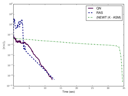
Fig. 12: QN, RAS, and $(\text{NEWT}\backslash\text{K}-\text{ASM})$ convergence.

Table 11: QN, RAS, and $(\text{NEWT}\backslash\text{K}-\text{ASM})$ results.

Solver	T	N. It	L. It	Func	Jac	PC	NPC
QN	12.24	2960	0	5921	–	–	–
RAS	12.94	352	0	1090	352	352	–
$(\text{NEWT}\backslash\text{K}-\text{ASM})$	34.57	124	3447	423	124	3574	–

Table 11 contains results for the uncomposed solvers. The default solver, $\text{NEWT}\backslash\text{K}-\text{ASM}$, takes a large number of outer Newton iterations and inner $\text{GMRES}-\text{ASM}$ iterations. In addition, the line search is consistently activated, causing an average of more than three function evaluations per iteration. Unpreconditioned QN is able to converge to the solution efficiently and will be hard to beat. QN stores up to 10 previous solutions and residuals. RAS set to do one local Newton iteration per subdomain per outer iteration proves to be efficient on its own after some initial problems, as shown in Fig. 12.

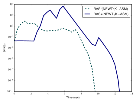
Fig. 13: $\text{RAS}*(\text{NEWT}\backslash\text{K}-\text{ASM})$ and $\text{RAS}+(\text{NEWT}\backslash\text{K}-\text{ASM})$ convergence.

Table 12: $\text{RAS}*(\text{NEWT}\backslash\text{K}-\text{ASM})$ and $\text{RAS}+(\text{NEWT}\backslash\text{K}-\text{ASM})$ results.

Solver	T	N. It	L. It	Func	Jac	PC	NPC
$\text{RAS}*(\text{NEWT}\backslash\text{K}-\text{ASM})$	9.69	24	750	142	48	811	–
$\text{RAS}+(\text{NEWT}\backslash\text{K}-\text{ASM})$	12.78	33	951	232	66	1023	–

In Table 12 and Fig. 13, we show how Newton’s method may be dramatically improved by composition with RAS and NASM. The additive composition reduces the number of outer iterations substantially. The multiplicative composition is even more effective, reducing the number of outer iterations by a factor of 5 and decreasing runtime by a factor of around 4.

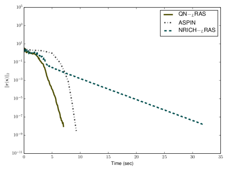
Fig. 14: $\text{QN}-_{L}\text{RAS}$ , ASPIN, and $\text{NRICH}-_{L}\text{RAS}$ convergence.

Table 13: $\text{QN}-_{L}\text{RAS}$ , ASPIN, and $\text{NRICH}-_{L}\text{RAS}$ results.

Solver	T	N. It	L. It	Func	Jac	PC	NPC
$\text{QN}-_{L}\text{RAS}$	7.02	92	0	410	185	185	185
ASPIN	9.30	13	332	307	179	837	19
$\text{NRICH}-_{L}\text{RAS}$	32.10	308	0	1889	924	924	924

The results for left-preconditioned methods are shown in Table 13 and Fig. 14. ASPIN is competitive, taking 13 iterations and having performance characteristics similar to those of the multiplicative composition solver listed in Table 12. The subdomain solvers for ASPIN are set to converge to a relative tolerance of $10^{-3}$ or 20 inner iterations. Underresolving the local problems provides an inadequate search direction and causes ASPIN to stagnate. The linear GMRES iteration also is converged to $10^{-3}$.

The most impressive improvements can be achieved by using a RAS as a nonlinear preconditioner. Simple NRICH acceleration does not provide much benefit compared with raw RAS with respect to outer iterations, and the preconditioner applications in the line search cause significant overhead. However, QN using inexact RAS as the left-preconditioned residual proves to be the most efficient solver for this problem, taking 185 Newton iterations per subdomain. Both NRICH and QN stagnate if the original residual is used in the line search instead of the preconditioned one. Subdomain QN methods [48] have been proposed before but built by using block approximate Jacobian inverses instead of working on the preconditioned system like ASPIN. As implemented here, $\text{QN}-_{L}\text{RAS}$ and ASPIN both construct left-preconditioned residuals and approximate preconditioned Jacobian constructions; both end up being very efficient.

7 Conclusion

The combination of solvers using nonlinear composition, when applied carefully, may greatly improve the convergence properties of nonlinear solvers. Hierarchical and multilevel inner solvers allow for high arithmetic intensity and low communication algorithms, making nonlinear composition a good option for extreme-scale nonlinear solvers.

Our experimentation, in this document and elsewhere, has shown that what works best when using nonlinear composition varies from problem to problem. Nonlinear composition introduces a slew of additional solver parameters at multiple levels of the hierarchy that may be tuned for optimal performance and robustness. A particular problem may be amenable to a simple solver, such as NCG, or to a combination of multilevel solvers, such as $\text{FAS}*(\text{NEWT}\backslash\text{K}-\text{MG})$. The implementation in PETSc [3] allows for considerable flexibility in user choice of solver compositions.

Admittedly, we have been fairly conservative in the scope of our solver combinations. Our almost-complete restriction to combinations of a globalized method and a decomposition method is somewhat artificial in the nonlinear case. Without this restriction, however, the combinatorial explosion of potential methods would quickly make the scope of this paper untenable. Users may experiment, for their particular problem, with combinations of some number of iterations of arbitrary combinations of nonlinear solvers, with nesting much deeper than we explore here.

The use of nonlinear preconditioning allows for solvers that are more robust to difficult nonlinear problems. While effective linear preconditioners applied to the Jacobian inversion problem may speed the convergence of the inner solves, lack of the convergence of the outer Newton’s method may doom the solve. With nonlinear preconditioning, the inner and outer treatment of the nonlinear problem allows for very rapid solution. Nonlinear preconditioning and composition solvers allow for both efficiency and robustness gains, and the widespread adoption of these techniques would reap major benefits for computational science.

Government License. The submitted manuscript has been created by UChicago Argonne, LLC, Operator of Argonne National Laboratory (“Argonne”). Argonne, a U.S. Department of Energy Office of Science laboratory, is operated under Contract No. DE-AC02-06CH11357. The U.S. Government retains for itself, and others acting on its behalf, a paid-up nonexclusive, irrevocable worldwide license in said article to reproduce, prepare derivative works, distribute copies to the public, and perform publicly and display publicly, by or on behalf of the Government.

References

- [1] Advanced Micro Devices, AMD Opteron 6200 series quick reference guide, 2012.
- [2] Donald G. Anderson, Iterative procedures for nonlinear integral equations, Journal of the ACM, 12 (1965), pp. 547–560.
- [3] Satish Balay, Shrirang Abhyankar, Mark F. Adams, Jed Brown, Peter Brune, Kris Buschelman, Victor Eijkhout, William D. Gropp, Dinesh Kaushik, Matthew G. Knepley, Lois Curfman McInnes, Karl Rupp, Barry F. Smith, and Hong Zhang, PETSc users manual, Tech. Report ANL-95/11 - Revision 3.5, Argonne National Laboratory, 2014.
- [4] Philipp Birken and Antony Jameson, On nonlinear preconditioners in Newton-Krylov methods for unsteady flows, International Journal for Numerical Methods in Fluids, 62 (2010), pp. 565–573.
- [5] J. H. Bramble, Multigrid Methods, Longman Scientific and Technical, Essex, England, 1993.
- [6] Achi Brandt, Multi-level adaptive solutions to boundary-value problems, Mathematics of Computation, 31 (1977), pp. 333–390.
- [7] Achi Brandt, Multigrid techniques: 1984 guide with applications for fluid dynamics, Tech. Report GMD-Studien Nr. 85, Gesellschaft fur Mathematik und Dataenverarbeitung, 1984.
- [8] A. Brandt and D. Ron, Multigrid solvers and multilevel optimization strategies, in Multilevel Optimization and VLSICAD, Kluwer Academic Publishers, 2003, pp. 1–69.
- [9] William L. Briggs, Van Emden Henson, and Steve F. McCormick, A Multigrid Tutorial (2nd ed.), Society for Industrial and Applied Mathematics, Philadelphia, PA, 2000.
- [10] Jed Brown and Peter Brune, Low-rank quasi-Newton updates for robust Jacobian lagging in Newton-type methods, in International Conference on Mathematics and Computational Methods Applied to Nuclear Science and Engineering, 2013, pp. 2554–2565.
- [11] P. Brown and A. Hindmarsh, Matrix-free methods for stiff systems of ODEs, SIAM Journal on Numerical Analysis, 23 (1986), pp. 610–638.
- [12] Peter N Brown and Youcef Saad, Convergence theory of nonlinear Newton-Krylov algorithms, SIAM Journal on Optimization, 4 (1994), pp. 297–330.
- [13] Charles G Broyden, A class of methods for solving nonlinear simultaneous equations, Mathematics of computation, 19 (1965), pp. 577–593.
- [14] RichardH. Byrd, Jorge Nocedal, and RobertB. Schnabel, Representations of quasi-Newton matrices and their use in limited memory methods, Mathematical Programming, 63 (1994), pp. 129–156.
- [15] X.-C. Cai, Nonlinear overlapping domain decomposition methods, Lecture Notes in Computational Science, 70 (2009), pp. 217–224.
- [16] X.-C. Cai and D. E. Keyes, Nonlinearly preconditioned inexact Newton algorithms, SIAM J. Sci. Comput., 24 (2002), pp. 183–200.
- [17] X.-C. Cai and X. Li, Inexact Newton methods with restricted additive Schwarz based nonlinear elimination for problems with high local nonlinearity, SIAM Journal on Scientific Computing, 33 (2011), pp. 746–762.
- [18] N. Carlson and K. Miller, Design and application of a gradient-weighted moving finite element code I: In one dimension, SIAM Journal on Scientific Computing, 19 (1998), pp. 728–765.
- [19] T. Chan and K. Jackson, Nonlinearly preconditioned Krylov subspace methods for discrete Newton algorithms, SIAM Journal on Scientific and Statistical Computing, 5 (1984), pp. 533–542.
- [20] Philippe Cresta, Olivier Allix, Christian Rey, and Stéphane Guinard, Nonlinear localization strategies for domain decomposition methods: Application to post-buckling analyses, Computer Methods in Applied Mechanics and Engineering, 196 (2007), pp. 1436–1446. Domain Decomposition Methods: recent advances and new challenges in engineering.
- [21] Y. H. Dai and Y. Yuan, A nonlinear conjugate gradient method with a strong global convergence property, SIAM Journal on Optimization, 10 (1999), pp. 177–182.
- [22] Hans De Sterck, Steepest descent preconditioning for nonlinear GMRES optimization, Numerical Linear Algebra with Applications, 20 (2013), pp. 453–471.
- [23] R. Dembo, S. Eisenstat, and T. Steihaug, Inexact Newton methods, SIAM Journal on Numerical Analysis, 19 (1982), pp. 400–408.
- [24] J. E. Dennis, Jr. and Jorge J. More, Quasi-Newton methods, motivation and theory, SIAM Review, 19 (1977), pp. 46–89.
- [25] J. E. Dennis Jr. and Robert B. Schnabel, Numerical Methods for Unconstrained Optimization and Nonlinear Equations, Prentice-Hall, Englewood Cliffs, NJ, 1983.
- [26] Peter Deuflhard, Roland Freund, and Artur Walter, Fast secant methods for the iterative solution of large nonsymmetric linear systems, IMPACT of Computing in Science and Engineering, 2 (1990), pp. 244–276.
- [27] Stanley C Eisenstat and Homer F Walker, Globally convergent inexact Newton methods, SIAM Journal on Optimization, 4 (1994), pp. 393–422.
- [28] V. Eyert, A comparative study on methods for convergence acceleration of iterative vector sequences, J. Comput. Phys., 124 (1996), pp. 271–285.
- [29] Haw-ren Fang and Yousef Saad, Two classes of multisecant methods for nonlinear acceleration, Numer. Linear Algebra Appl., 16 (2009), pp. 197–221.
- [30] Roger Fletcher, Practical Methods of Optimization, Volume 1, Wiley, 1987.
- [31] R. Fletcher and C. M. Reeves, Function minimization by conjugate gradients, Computer Journal, 7 (1964), pp. 149––154.
- [32] Allen A Goldstein, On steepest descent, Journal of the Society for Industrial & Applied Mathematics, Series A: Control, 3 (1965), pp. 147–151.
- [33] W. Hackbusch, Comparison of different multi-grid variants for nonlinear equations, ZAMM - Journal of Applied Mathematics and Mechanics / Zeitschrift für Angewandte Mathematik und Mechanik, 72 (1992), pp. 148–151.
- [34] Van E. Henson, Multigrid methods for nonlinear problems: an overview, Proc. SPIE, 5016 (2003), pp. 36–48.
- [35] Magnus R. Hestenes and Eduard Steifel, Methods of conjugate gradients for solving linear systems, J. Research of the National Bureau of Standards, 49 (1952), pp. 409–436.
- [36] J. D. Hunter, Matplotlib: A 2d graphics environment, Computing In Science & Engineering, 9 (2007), pp. 90–95.
- [37] F.-N. Hwang and X.-C. Cai, A parallel nonlinear additive Schwarz preconditioned inexact Newton algorithm for incompressible Navier-Stokes equations, J. Comput. Phys., 204 (2005), pp. 666–691.
- [38] C. T. Kelley, Iterative Methods for Linear and Nonlinear Equations, SIAM, Philadelphia, 1995.
- [39] C. T. Kelley and D.E. Keyes, Convergence analysis of pseudo-transient continuation, SIAM J. Numerical Analysis, 35 (1998), pp. 508–523.
- [40] Hector Klie and Mary F Wheeler, Nonlinear Krylov-secant solvers, tech. report, Dept. of Mathematics and inst. of Computational Engineering and Sciences, University of Texas at Austin, 2006.
- [41] D. Knoll and P. McHugh, Enhanced nonlinear iterative techniques applied to a nonequilibrium plasma flow, SIAM Journal on Scientific Computing, 19 (1998), pp. 291–301.
- [42] D. A. Knoll and D. E. Keyes, Jacobian-free Newton-Krylov methods: A survey of approaches and applications, J. Comp. Phys., 193 (2004), pp. 357–397.
- [43] P. Ladevèze, J.-C. Passieux, and D. Néron, The LATIN multiscale computational method and the proper generalized decomposition, Computer Methods in Applied Mechanics and Engineering, 199 (2010), pp. 1287 – 1296. Multiscale Models and Mathematical Aspects in Solid and Fluid Mechanics.
- [44] P. Ladevèze and J.G. Simmonds, Nonlinear computational structural mechanics: New approaches and non-incremental methods of calculation, Mechanical Engineering Series, Springer, 1999.
- [45] Paul J Lanzkron, Donald J Rose, and James T Wilkes, An analysis of approximate nonlinear elimination, SIAM Journal on Scientific Computing, 17 (1996), pp. 538–559.
- [46] Dong C Liu and Jorge Nocedal, On the limited memory BFGS method for large scale optimization, Mathematical Programming, 45 (1989), pp. 503–528.
- [47] P. A. Lott, H. F. Walker, C. S. Woodward, and U. M. Yang, An accelerated Picard method for nonlinear systems related to variably saturated flow, Advances in Water Resources, 38 (2012), pp. 92–101.
- [48] José Mario Martínez, SOR-secant methods, SIAM J. Numer. Anal., 31 (1994), pp. 217–226.
- [49] Hermann Matthies and Gilbert Strang, The solution of nonlinear finite element equations, International Journal for Numerical Methods in Engineering, 14 (1979), pp. 1613–1626.
- [50] Stephen G Nash, A multigrid approach to discretized optimization problems, Optimization Methods and Software, 14 (2000), pp. 99–116.
- [51] Jorge Nocedal, Updating quasi-Newton matrices with limited storage, Mathematics of Computation, 35 (1980), pp. 773–782.
- [52] Jorge Nocedal and Stephen J. Wright, Numerical Optimization, Springer-Verlag, New York, 1999.
- [53] E Polak and G Ribiere, Note sur la convergence de méthodes de directions conjuguées, Revue française d’informatique et de recherche opérationnelle, série rouge, 3 (1969), pp. 35–43.
- [54] Péter Pulay, Convergence acceleration of iterative sequences: The case of SCF iteration, Chemical Physics Letters, 73 (1980), pp. 393–398.
- [55] Alfio Quarteroni and Alberto Valli, Domain Decomposition Methods for Partial Differential Equations, Oxford Science Publications, Oxford, 1999.
- [56] P. Ramachandran and G. Varoquaux, Mayavi: 3D Visualization of Scientific Data, Computing in Science & Engineering, 13 (2011), pp. 40–51.
- [57] Youcef Saad, A flexible inner-outer preconditioned GMRES algorithm, SIAM Journal on Scientific Computing, 14 (1993), pp. 461–469.
- [58] Yousef Saad, Iterative Methods for Sparse Linear Systems, 2nd edition, SIAM, Philadelpha, PA, 2003.
- [59] Michael H Scott and Gregory L Fenves, A Krylov subspace accelerated Newton algorithm, in Proc., 2003 ASCE Structures Congress, 2003.
- [60] D. F. Shanno, Conditioning of quasi-Newton methods for function minimization, Mathematics of Computation, 24 (1970), pp. pp. 647–656.
- [61] Jonathan R Shewchuk, An introduction to the conjugate gradient method without the agonizing pain, tech. report, Carnegie Mellon University, Pittsburgh, PA, 1994.
- [62] B.F. Smith, Domain decomposition methods for partial differential equations, ICASE LARC Interdisciplinary Series in Science and Engineering, 4 (1997), pp. 225–244.
- [63] Barry F. Smith, Petter Bjørstad, and William D. Gropp, Domain Decomposition: Parallel Multilevel Methods for Elliptic Partial Differential Equations, Cambridge University Press, 1996.
- [64] B. F. Smith and X. Tu, Encyclopedia of Applied and Computational Mathematics, Springer, 2013, ch. Domain Decomposition.
- [65] M.D. Smooke and R.M.M. Mattheij, On the solution of nonlinear two-point boundary value problems on successively refined grids, Applied Numerical Mathematics, 1 (1985), pp. 463 – 487.
- [66] Andrea Toselli and Olof B Widlund, Domain Decomposition Methods: Algorithms and Theory, vol. 34, Springer, 2005.
- [67] U. Trottenberg, C.W. Oosterlee, and A. Schüller, Multigrid, Academic Press, 2001.
- [68] Raymond S Tuminaro, Homer F Walker, and John N Shadid, On backtracking failure in Newton–GMRES methods with a demonstration for the Navier–Stokes equations, Journal of Computational Physics, 180 (2002), pp. 549–558.
- [69] Homer F. Walker and Peng Ni, Anderson acceleration for fixed-point iterations, SIAM J. Numer. Anal., 49 (2011), pp. 1715–1735.
- [70] Homer F Walker, Carol S Woodward, and Ulrike M Yang, An accelerated fixed-point iteration for solution of variably saturated flow, in Proc. XVIII International Conference on Water Resources, Barcelona, 2010.
- [71] T Washio and CW Oosterlee, Krylov subspace acceleration for nonlinear multigrid schemes, Electronic Transactions on Numerical Analysis, 6 (1997), pp. 271–290.
- [72] T. Washio and C. W. Oosterlee, Krylov subspace acceleration for nonlinear multigrid schemes with application to recirculating flow, SIAM Journal on Scientific Computing, 21 (2000), pp. 1670–1690.
- [73] Pieter Wesseling, An Introduction to Multigrid Methods, R. T. Edwards, 2004.
- [74] P. Wolfe, Convergence conditions for ascent methods, SIAM Review, 11 (1969), pp. 226–235.
- [75] Peter Wriggers, Nonlinear Finite Element Methods, Springer, 2008.