Pseudomagnetic fields for sound at the nanoscale

Abstract

There is a growing effort in creating chiral transport of sound waves. However, most approaches so far are confined to the macroscopic scale. Here, we propose a new approach suitable to the nanoscale which is based on pseudo-magnetic fields. These fields are the analogue for sound of the pseudo-magnetic field for electrons in strained graphene. In our proposal, they are created by simple geometrical modifications of an existing and experimentally proven phononic crystal design, the snowflake crystal. This platform is robust, scalable, and well-suited for a variety of excitation and readout mechanisms, among them optomechanical approaches.

A novel trend has emerged recently in the design of mechanical systems, towards incorporating topological ideas. These ideas promise to pave the way towards transport along edge-channels that are either purely uni-directional Nash2015 or helical Susstrunk2015 (i.e. with two “spins” moving in opposite directions), as well as the design of novel zero-frequency boundary modes Kane2013 ; Paulose2015 . The first few experimental realizations Susstrunk2015 ; Paulose2015 ; Nash2015 ; Xiao2015 ; He2015arXiv ; RocklinarXiv2015 ; Chen2014 and a number of theoretical proposals Kane2013 ; Yang2015 ; Khanikaev2015 ; Kariyado2015 ; Bertoldi2015 ; Pal2016 ; Fleury2016 ; Mei2016 ; Chen2016 ; Rocklin2016 ; sussman2016 involve macroscopic setups. These include coupled spring systems Prodan2009 ; Bertoldi2015 ; Susstrunk2015 ; Nash2015 ; Kariyado2015 ; Pal2016 and circulating fluids Yang2015 ; Khanikaev2015 ; Chen2016 ; Lu2016 for a review Susstrunk2016 . These designs represent important proof-of-principle demonstrations of topological acoustics and could open the door to useful applications at the macroscopic scale. However, they are not easily transferred to the nanoscale, which would be even more important for potential applications.

The first proposal for engineered chiral sound wave transport at the nanoscale has been put forward in Ref. Peano2015 : an appropriately patterned slab illuminated by a laser with a suitably engineered wavefront realizes a Chern insulator for sound. The laser drive in Peano2015 breaks the time-reversal symmetry, enabling uni-directional topologically protected transport. On the other hand, there would be clear practical advantages of a design that operates without any drive and, at the same time, in a simple nanoscale geometry. By necessity, this must result in helical transport, with two counter-propagating species of excitations.

There are two important classes in this regard: (i) topological insulators, and (ii) pseudo-magnetic fields. A first idea for (i) at the nanoscale was put forward recently in Ref. Mousavi2015 . By contrast, in the present paper, we show how to engineer arbitrary spatial pseudo-magnetic field distributions for sound waves in a purely geometry-based design. In addition (and again in contrast to Mousavi2015 ), it turns out that our design can be implemented in a platform that has already been realized and reliably operated at the nanoscale, the snowflake phononic crystal SafaviNaeini2014 . That platform has the added benefit of being a well-studied optomechanical system, which, as we will show, can also provide powerful means of excitation and readout. The mechanical pseudo-magnetic fields are analogous to the pseudo-magnetic fields for electrons propagating on the curved surface of carbon nanotubes Kane1997 and in strained graphene Manes2007 ; Guinea2010 ; Levy2010 ; Low2010 . Pseudo-magnetic fields mimic real magnetic fields, but have opposite sign in the two valleys of the graphene band structure and, thus, do not break time-reversal symmetry. In the past, this concept has already been successfully transferred to a photonic waveguide system Rechtsman2013 .

Besides presenting our nanoscale design, we also put forward a general approach to pseudo-magnetic fields for Dirac quasiparticles based on the smooth breaking of the ${\cal C}_{6}$ point group and translational symmetries. Our scheme is especially well suited to patterned engineered materials such as phononic and photonic crystals. It ties into the general efforts of steering sound in acoustic metamaterials at all scales Maldovan2013 ; Popa2011 ; Khelif_Book ; Ma2015 .

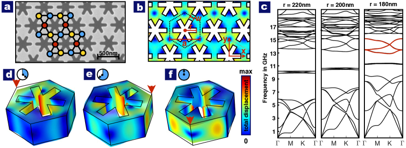
Figure 1: Snowflake crystal: geometry, band structure and displacement fields. (a) Image of a silicon snowflake phononic crystal. It is formed by upwards and downwards triangles connected by links. The links form a Kagome lattice whose Bravais sublattices are marked by circles of different colors. (b) Top view of the field $|\boldsymbol{\psi}_{m_{s},\tau}(\mathbf{x},z)|^{2}$ (time-averaged square displacement) for one normal mode at the Dirac point ($m_{s}=-1$ and valley $\tau=-1$). The dashed line indicates the border of the Wigner-Seitz cell. The relevant geometric parameters are indicated. (c) Phononic band structure ($z$-symmetric modes) for three values of the snowflake radius $r$, in silicon. The band structure is computed using a finite-element solver (COMSOL). The slab thickness is 220nm and the remaining geometry parameters, c.f. panel (b), are (a,w)=(500,75)nm. For $r=180$nm, a group of three bands (plotted in red) is separated by complete band gaps from the remaining bands. The triplet is well fitted by a Kagome lattice model and exhibits Dirac cones at the high symmetry points $\mathbf{K}$ and $\mathbf{K^{\prime}}$ (only $\mathbf{K}$ is shown). At the cone tip, the degenerate normal modes have quasi-angular momentum $m_{s}=\pm 1$. (d–f) Snapshots of the mechanical displacement field (absolute value encoded in the color scale) for the mode with quasi-angular momentum $m_{s}=-1$ and valley $\tau=-1$, within a Wigner-Seitz cell. Subsequent snapshots are taken after one third of a period (cf. the clocks). Each snapshot is the anti-clockwise rotation by a $2\pi/3$ angle around the snowflake center of the previous snapshot (cf. the arrows).

Dirac equation and gauge fields – The $2D$ Dirac Hamiltonian in the presence of a gauge field $\mathbf{A}(\mathbf{x})$ reads (we set the Planck constant and the charge equal to one) Neto2009

$$\hat{H}_{D}=m\hat{\sigma}_{z}+v(p_{x}-A_{x}(\mathbf{x}))\hat{\sigma}_{x}+v(p_{y}-A_{y}(\mathbf{x}))\hat{\sigma}_{y}.$$ (1)

Here, $m$ is the mass, $v$ is the Dirac velocity, and $\hat{\sigma}_{x,y,z}$ are the Pauli matrices. For zero mass and a constant gauge field ($m=0$ and $\mathbf{A(\mathbf{x})}=\mathbf{A}$), the band structure forms a Dirac (double) cone, where the top and bottom cones touch at the momentum $\mathbf{p}=\mathbf{A}$.

In a condensed matter setting, the Dirac Hamiltonian describes the dynamics of a particle in a honeycomb lattice, or certain other periodic potentials, within a quasimomentum valley, i.e. within the vicinity of a lattice high-symmetry point in the Brillouin zone. In this context, $\mathbf{p}$ is the quasi momentum counted off from the relevant high-symmetry point. Here, we are interested in a scenario where the Dirac Hamiltonian Eq. (1) is defined in two different valleys mapped into each other via the time-reversal symmetry operator ${\cal T}$. This scenario is realized in graphene, where the Dirac equation is defined in the two valleys around the symmetry points $\mathbf{K}$ and $\mathbf{K^{\prime}}$. For charged particles, the gauge field $\mathbf{A}(\mathbf{x})$ usually describes a real magnetic field $\mathbf{B}$, where $\mathbf{B}=\nabla\times\mathbf{A}$. In this case, the time-reversal symmetry ${\cal T}$ is broken. For $m=0$ and a constant magnetic field, the Dirac cones break up in a series of flat Landau levels Neto2009 ,

$$E_{n}={\rm sign}(n)\sqrt{|n|}\omega_{c},\quad\omega_{c}=v\sqrt{2B},$$ (2)

where $n\in Z$ and $\omega_{c}$ is the cyclotron frequency. The presence of a physical edge then leads to topologically protected gapless edge states in each valley. For a real magnetic field, the edge states in the two valleys have the same chirality. However, here, we will be interested in the case of engineered pseudo-magnetic fields, where the gauge field $\mathbf{A}(\mathbf{x})$ does not break the ${\cal T}$-symmetry. In this case, $\mathbf{B}=\nabla\times\mathbf{A}$ must have opposite sign in the two different valleys to preserve the ${\cal T}$-symmetry. It is clear that as long as one can focus on a single valley, the nature of the magnetic field (real or pseudo magnetic field) does not play any role. This holds true also in the presence of boundaries. For a given valley and gauge potential $\mathbf{A}$, exactly the same edge excitations will emerge in the presence of a pseudo- or a real magnetic field. The nature of the magnetic field only becomes apparent when the eigenstates belonging to inequivalent valleys are compared. When time-reversal is preserved (pseudo magnetic field), each edge state in one valley has a time-reversed partner with opposite velocity in the other valley. Thus, the edge states induced by a pseudo magnetic field are not chiral but rather helical.

Dirac phonons in the snowflake phononic crystal – FEM mechanical simulations of a silicon thin-film snowflake crystal are presented in Figure 1. Throughout this work, we restrict our attention to the modes that are even under the mirror symmetry $(x,y,z)\rightarrow(x,y,-z)$, i.e. the $z$-symmetric modes. The mechanical band structure is shown in Fig. 1c. It features a large number of Dirac cones at the high-symmetry point $\mathbf{K}$. Each cone has a time-reversed partner at the point $\mathbf{K}^{\prime}$ (not shown). These pairs of Dirac cones are robust structures: when the radius of the snowflake is varied, they are shifted in energy (and can possibly cross other bands) but the top and bottom cones always touch at the corresponding high-symmetry point, see panel c. In other words, the mass $m$ and the gauge field $\mathbf{A}$ are always zero in the corresponding Dirac Hamiltonian. In order to generate the desired gauge field, it is necessary to modify the pattern of holes in a way that breaks the symmetries of the crystal (see discussion below).

In preparation of this, we use the snowflake radius as a knob to engineer a pair of Dirac cones which are spectrally well isolated from other bands and have a large velocity. The snowflake crystal can be viewed as being formed by an array of triangular membranes arranged on a honeycomb lattice and connected through links (see Figure 1b). In principle, we could choose a situation where the links are narrow (large snowflake radius $r$), such that all the groups of bands are spectrally well isolated. However, then the Dirac velocities tend to be small. For wider links (smaller $r$), the motion of the adjacent edges of neighboring triangular membranes becomes strongly coupled. This give rise to normal modes where such adjacent sides oscillate in phase, resulting in large displacements of the links. We note that these links are arranged on a Kagome lattice, see Figure 1a. This observation explains the emergence (see r=180nm plot of Fig. 1e) of a group of three bands, separated from the remaining bands by complete band gaps, and supporting large velocity Dirac cones. The triplet of isolated bands can be well fitted by a Kagome lattice tight-binding model with nearest-neighbor and next-nearest neighbor hopping. The Kagome lattice model would be entirely sufficient to guide us in the engineering of the desired gauge fields. However, we prefer to pursue a more fundamental and general approach based on the symmetries of the underlying snowflake crystal.

Identifying the Dirac pseudo-spin by the symmetries – The snowflake thin-film slab crystal has ${\cal D}_{6h}$ point group symmetry. If we restrict our attention to the $z$-symmetric modes, the remaining point group is ${\cal C}_{6v}$ (six-fold rotations about the snowflake center and mirror symmetries about the vertical planes containing a lattice basis vector). The degeneracies underpinning the Kagome Dirac cones as well as the other robust cones in Fig. 1b are usually referred to as essential degeneracies. They are preserved if the point group includes at least the ${\cal C}_{6}$ symmetries (six-fold rotational symmetry about the snowflake center) or the ${\cal C}_{3v}$ symmetries (three-fold rotations and mirror symmetries about three vertical planes containing a lattice unit vector). The point group here contains both groups but, for concreteness, our explanation will focus on the ${\cal C}_{6}$ symmetry. It is useful to think of the ${\cal C}_{6}$ symmetry as a combination of a ${\cal C}_{3}$ (three-fold) symmetry group and a ${\cal C}_{2}$ (two-fold) symmetry group. The three-fold rotations ${\cal C}_{3}$ belong to the group of the high-symmetry points $\mathbf{K}$ and $\mathbf{K}^{\prime}$ (they leave each of these point invariant modulo a reciprocal lattice vector). As a consequence, at these points, the eigenmodes can be chosen to be eigenvectors of the ${\cal C}_{3}$ rotations with quasi-angular momentum $m_{{\rm s}}=0,\pm 1$. The essential degeneracies come about because the eigenvectors with non-zero quasi-angular momentum $m_{s}$ come in quadruplets (a degenerate pair in each inequivalent valley), mapped into each other via the time-reversal symmetry operator ${\cal T}$ and the rotation $\hat{R}(\pi)_{z}$ by $180^{o}$ about the snowflake center (the sole non-trivial element of the ${\cal C}_{2}$ group). If we denote the members of a quadruplet by $\boldsymbol{\psi}_{m_{s},\tau}(\mathbf{x},z)$, where $m_{s}=\pm 1$ and $\tau=\pm 1$ indicates the valley and $z$ is the vertical coordinate, we have

$$\mathbf{\boldsymbol{\psi}}_{m_{s},\tau}={\cal T}\mathbf{\boldsymbol{\psi}}_{-m_{s},-\tau}=\hat{R}(\pi)_{z}\mathbf{\boldsymbol{\psi}}_{m_{s},-\tau}={\cal T}\hat{R}(\pi)_{z}\mathbf{\boldsymbol{\psi}}_{-m_{s},\tau}.$$

Note that both ${\cal T}$ and $R(\pi)$ change the sign of the quasimomentum and, thus, of $\tau$. However, only ${\cal T}$ changes the sign of the quasi-angular momentum.

The Dirac Hamiltonian (1) for a given valley $\tau$ is obtained by projecting the underlying elasticity equations onto a two-dimensional Hilbert space spanned by the normal modes

$$\boldsymbol{\psi}_{\mathbf{p},m_{s},\tau}(\mathbf{x},z)=e^{i\mathbf{p}\cdot\mathbf{x}}\boldsymbol{\psi}_{m_{s},\tau}(\mathbf{x},z),$$ (3)

and by identifying $-m_{s}=\pm 1$ with the eigenvalues of the $\hat{\sigma}_{z}$ matrix (see Appendix B). In other words, the quasi-angular momentum $m_{s}$ plays the role of the Dirac pseudospin. A mass term is forbidden because states with equal quasimomentum and opposite quasi-angular momentum are mapped into each other by the symmetry ${\cal T}\hat{R}(\pi)_{z}$, $\boldsymbol{\psi}_{\mathbf{p},m_{s},\tau}(\mathbf{x},z)={\cal T}\hat{R}(\pi)_{z}\boldsymbol{\psi}_{\mathbf{p},-m_{s},\tau}(\mathbf{x},z)$. A gauge field $\mathbf{A}$ is also forbidden because it would couple states with different quasi-angular momentum at the symmetry point.

In our phononic Dirac system, the eigenstates $\boldsymbol{\psi}_{m_{s},\tau}(\mathbf{x},z)$ are three-dimensional complex vector fields. They yield the displacement fields,

$$\mathbf{u}_{m_{s},\tau}(\mathbf{x},z,\phi)={\rm Re}[\exp(-i\phi)\mathbf{\boldsymbol{\psi}}_{m_{s},\tau}(\mathbf{x},z)]$$ (4)

where $\phi$ is the phase of the oscillation. In this classical setting, $|\boldsymbol{\psi}_{m_{s},\tau}(\mathbf{x},z)|^{2}$ can be interpreted as the square displacement averaged over one period, $|\boldsymbol{\psi}_{m_{s},\tau}(\mathbf{x},z)|^{2}=\pi^{-1}\int_{0}^{2\pi}d\phi|\mathbf{u}_{m_{s},\tau}(\mathbf{x},z,\phi)|^{2}$. We note that the field $|\boldsymbol{\psi}_{m_{s},\tau}(\mathbf{x},z)|^{2}$ is invariant under threefold rotations about three inequivalent rotocenters: the center of the snowflake and the centers of the downwards and upwards triangles (see Figure 1b). Three snapshots of the instantaneous displacement field for the state with $m_{s}=-1$ and $\tau=-1$ are shown in Fig. 1d–f. By definition of a quasi-angular momentum eigenstate with $m_{s}=-1$, when the phase $\phi$ varies by $2\pi/3$ (after one third of a period), the instantaneous displacement field is simply rotated clockwise by the same angle. When the valley is known, the quasi-angular momentum (which here play the role of the pseudospin) can be directly read off from a single snapshot based on the position of the nodal lines. For $m_{s}\tau=1$ $(m_{s}\tau=-1)$, they are located at the center of the downwards (upwards) triangles, cf. Fig. 1b,d–f. (For a detailed explanation see Appendix B). Below, we will take advantage of our insight on the symmetries of the pseudospin eigenstates to engineer a local force field which selectively excites uni-directional waves.

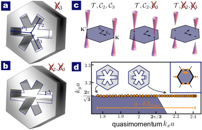
Figure 2: Snowflake geometry and Dirac cones: (a) Geometry of the snowflake unit cell, depicting a situation with a broken three-fold rotational symmetry ${\cal C}_{3}$ but preserved two-fold rotational symmetry ${\cal C}_{2}$ ($r_{1}\neq r_{2}=r_{3}$). (b) Geometry where both ${\cal C}_{3}$ and ${\cal C}_{2}$ symmetries are broken (a snowflake arm is displaced vertically by $\Delta$). (c) Resulting shape of the Dirac cones. Breaking ${\cal C}_{3}$, while time-reversal symmetry $\mathcal{T}$ and ${\cal C}_{2}$ are maintained, leads to gapless cones displaced from the high-symmetry points. When also the ${\cal C}_{2}$ symmetry is broken, a band gap (mass) separating the upper and lower cones appears. (d) Displacement of the Dirac cone for the valley $\tau=-1$, for the geometry in panel (a) when $r_{1}$ is varied from $160$nm to $200$nm, while $r_{2}=r_{3}$ and $\bar{r}=(r_{1}+r_{2}+r_{3})/3=180\text{nm}.$

Pseudo-magnetic fields and symmetry-breaking – A crucial step towards the engineering of a pseudo-magnetic field is the implementation of a spatially constant vector potential $\mathbf{A}$ in a translationally invariant system. Afterwards arbitrary magnetic field distributions can be generated straightforwardly by breaking the translational invariance smoothly.

A perturbation that breaks the ${\cal C}_{3}$ symmetry but preserves the ${\cal C}_{2}$ symmetry will simply shift the Dirac cones, without opening a gap (see Figure 2c). This can be identified with the appearance of a constant gauge field $\mathbf{A}$ in the Dirac Hamiltonian (1). As such, the connection between changes in the microscopic structure of the phononic metamaterial and the resulting gauge field can be obtained from FEM simulations by extracting the quasimomentum shift of the Dirac cones. We emphasize that, in this context, the vector potential $\mathbf{A}$ has the dimension of an inverse length.

In the snowflake phononic crystal, we can achieve the desired type of symmetry breaking (breaking ${\cal C}_{3}$ while preserving ${\cal C}_{2}$) by designing asymmetric snowflakes formed by arms of different lengths, $r_{1},$ $r_{2},$ $r_{3}$ (see Figure 2a). If only one of the arms is changed, symmetry requires that the vector potential $\mathbf{A}$ points along that arm as shown in Fig. 2d. For the Dirac cones associated with the Kagome lattice, our FEM simulations show that the cone displacement grows linearly with the length changes, as long as these remain much smaller than the average arm length $r=(r_{1}+r_{2}+r_{3})/3$. In this linear regime, and for a general combination of arm lengths, $r_{1},$ $r_{2},$ $r_{3}$, we have

$$\mathbf{A}\approx\tau f(r)\mathbf{d},\quad\mathbf{d}=(r_{1}\mathbf{e}_{1}+r_{2}\mathbf{e}_{2}+r_{3}\mathbf{e}_{3}).$$ (5)

The unit vectors $\mathbf{e}_{j}$ point into the direction of the corresponding snowflake arms, $\mathbf{e}_{j}=\cos\theta_{j}\mathbf{e}_{x}+\sin\theta_{j}\mathbf{e}_{y}$, where $\theta_{j}=2\pi(j-1)/3$. The factor $\tau=\pm 1$ appears because the vector potential has opposite sign in the two valleys as we have not broken time reversal symmetry. We note that in general changes of the arm lengths also shift the frequency of the Dirac point. When the arm lengths are chosen to be position dependent, as is required for implementing arbitrary magnetic fields, this energy shift will enter the Dirac equation as a scalar potential $V(\mathbf{x})$, which may be unwanted. However, our numerical simulations show that we can keep $V(\mathbf{x})$ approximately constant, by retaining a constant average arm length $r$.

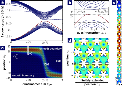
Figure 3: Band structure and displacement fields of a strip in a constant pseudo-magnetic field: (a) Band structure (only the $z$-symmetric modes are shown) and (b) zoom-in of the valley $\tau=-1$. The band structure displays multiple flat Landau plateaus in the vicinity of the $\mathbf{K}$’-point ($k_{x}a=2\pi/3$). In (b), the dashed lines indicate the energies of the Landau levels as calculated from the Dirac equation for mass $m=0$, cf. Eq. (2). In (a,b), the dot-dashed bands correspond to intrinsic non-chiral edge states located at the physical boundary of the system (see Appendix E). (c) Mode shape of the 0-th Landau level and the ensuing edge states (marked in red in panels a,b) as a function of the quasimomentum $k_{x}$. The region of the smooth boundaries (where $m\neq 0$) is marked in grey and the magnetic length $\ell_{B}$ in white. (d) Zoom-in of the displacement field of the $n=0$ Landau level. At the lattice scale, the displacement field pattern encodes the pseudospin $m_{s}=1$ of the Landau level (cf. Figure 1f). (e) Zoom-in of the edge state displacement field.

Phononic Landau levels and Edge States in a Strip – We can test these concepts by implementing a constant phononic pseudo-magnetic field in an infinite snowflake crystal strip, where we can directly test our simplified description against full microscopic simulations. The strip is of finite width $W$ in the $y$-direction (where $-W/2<y<W/2$). We can realize the corresponding vector potential in the Landau gauge, $\mathbf{A}(\mathbf{x})=(-B_{z}y,0,0)$, by varying the length $r_{1}$ along the $x$-axis, while keeping the remaining arm lengths equal, $r_{2}=r_{3}$. For concreteness we choose $B_{z}>0$ for $\tau=-1$.

The treatment of the boundaries merits special consideration. It turns out that sharp boundaries are unfavorable, as they give rise to an extra undesired edge mode that is not related to the quantum Hall effect physics that we seek to implement. Any smooth gradient of snowflake parameters near the boundaries of the sample will lead to well-defined edge states that are spatially separated from the physical system edge. In general, this could involve both a potential gradient as well as a gradient in the effective mass (gap). In our simulations, we will display results obtained for a smooth mass gradient, whose details do not matter for the qualitative behavior. A Dirac mass term appears upon breaking the ${\cal C}_{2}$ symmetry, which we here choose to do by transversally displacing one of the snowflake arms, as shown inFig. 2b, with the displacement varying smoothly in the interval $W_{{\rm bulk}}/2<|y|<W/2$.

By changing the snowflake arm lengths we can displace the Dirac cones only over a finite range of quasimomenta. In our simulations $\delta A_{{\rm max}}\approx 0.17\pi/a$, as shown in Fig. 2d. Using Eq. (2) and the definition of the magnetic length $\ell_{B}=B^{-1/2}$, we see that there is a trade-off between the cyclotron frequency $\omega_{c}$ and, thus, the achievable magnetic band gaps and the system size in the appropriate magnetic units: $\omega_{c}\leq\sqrt{2}v\delta A_{{\rm max}}/w$ where $w=W/\ell_{B}.$ For our FEM simulations we have chosen $w=6.2$.

In Fig. 3, we display the phonon band structure and the phonon wave functions (mechanical displacement fields) extracted from finite-element numerical simulations as a function of the quasimomentum $k_{x}$ along the translationally invariant (infinite) direction. We display only positive $k_{x}$ because, due to time-reversal symmetry, both the frequencies and the displacement fields are even functions of $k_{x}$. In the bulk, we expect to reproduce the well-known physics of Dirac materials in a constant (pseudo)-magnetic field Neto2009 . Indeed, the numerically extracted band structure consists of a series of flat Landau Levels at energies of precisely the predicted form $\omega=\bar{E}+E_{n}$ [$E_{n}$ is defined in Eq. (2)]; see panel (a) and the zoom-in (b) of Fig. 3. The Landau plateaus extend over a quasi momentum interval of width $\delta k_{x}\approx\delta A_{{\rm bulk}}=W_{{\rm bulk}}B$. Furthermore, in the bulk, we expect the mechanical eigenstates to be localized states of size $\ell_{B}=B^{-1/2}$ (in the $y$-direction). Their quasi momentum $k_{x}$ should be related to the position via $\bar{y}=-[k_{x}-2\pi/(3a)]/B_{z}$. This behavior is clearly visible in Fig. 3c, where we show the displacement field of the central Landau level. A zoom-in of this field (panel d) reveals that, at the lattice scale, it displays the same intensity pattern as the bulk pseudospin eigenstate $m_{s}=-1$ shown previously in Fig. 1f. This behavior is also predicted by the effective Dirac description where the central Landau level is indeed a pseudo-spin eigenstate with $m_{s}=-1$ when the magnetic field $B_{z}$ is positive Neto2009 . Note that the pseudo-magnetic field engineered here also gives rise to a Lorentz force that will curve the trajectory of phonon wavepackets traveling in the bulk of the sample. The sign of the force is determined by the valley index $\tau$.

Having demonstrated that we can implement a constant phononic pseudo-magnetic field, we now argue that our approach with smooth boundaries gives additional flexibility in the engineering of helical phononic waveguides. Each Landau level gives rise to an edge state in the region of the smooth boundaries. The typical behavior of the wavefunction is shown (for $n=0$) in Figure 3c. For decreasing quasimomenta $k_{x}$, an edge state localized on the lower edge smoothly evolves into a bulk state, and eventually into an edge state localized on the upper edge. As is clear from Fig. 3a and 3b, these pairs of edge states span the same energy interval. This behavior clearly leads to the same number of edge states (for a fixed energy) on both edges. This is crucial in view of engineering smooth helical transport on a closed loop. We emphasize that the number of states on the two edges need not necessarily (by symmetry) be equal. Indeed, graphene in a constant pseudo-magnetic field supports a different number of edge states on two opposite (sharp) edges Low2010 . In our approach, we can tune the number of edge states on each edge via the mass term. In particular, the behavior of the edge states originating from the $n=0$ Landau level is sensitive to the sign of the mass. A negative mass (as in our simulations) drags this Landau level into the band gap below. Vice versa, a positive mass will drag it into the band gap above. This behavior is related to the peculiarity of the Landau level being a pseudospin eigenstate (with $m_{s}=-1$) and, thus, an eigenstate of the mass term (with eigenvalue $m$), cf. Eq. (1).

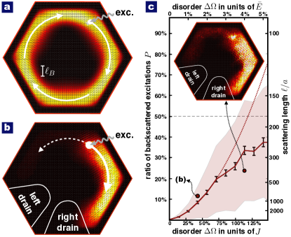
Figure 4: Tight-binding transport simulations in a finite geometry: The hexagon (height 55 unit cells) comprises an internal bulk area (height 45 unit cells) and external smooth boundaries. An engineered oscillating force (at the position indicated by the grey arrow) with frequency in the middle of a band gap (separating the Landau levels $n=-1$ and $n=0$) launches clockwise propagating sound waves. (a) Resulting displacement field (unit-cell resolved). (b) and inset of (c) Displacement field in the presence of disorder and drains where the excitation are absorbed. (c) Probability $P$ (averaged over 150 disorder implementations) that an excitation is absorbed in the left drain as a function of the disorder strength. The estimated error is represented by error bars. The shaded area represents the values of $P$ within one standard deviation. In the tight-binding model, the random onsite energies are equally distributed on an interval of width $\Delta\Omega$. For weak disorder ($\Delta\Omega/J\lesssim 70\%$ where $J$ is the average hopping rate), $P$ is well fitted by a parabola (dashed line), indicating that the transport is quasi-ballistic. In this regime, the corresponding scattering length $\ell$ is shown in the right vertical axis.

Transport in a Finite Geometry and Disorder – Any pseudo-magnetic field that is realized without explicit time-reversal symmetry breaking necessarily gives rise to helical transport, where the chirality depends on some artificial spin degree of freedom, i.e. the valley. A central question in this regard is the robustness against short-range disorder. In order to assess this, we have studied numerically transport in a finite geometry. As presented in Fig. 4, we consider a sample of hexagonal shape with smooth boundaries in the presence of a constant pseudo-magnetic field (we choose the symmetric gauge for the vector potential ${\bf A}$). In this illustrative example, a local probe drive excites vibrations near the boundaries, as indicated in Fig. 4a. Its frequency is chosen to lie inside the bulk band gap separating the $n=0$ and $n=-1$ Landau levels. In this band gap, the system supports a pair of counter-propagating helical edge states belonging to opposite valleys. One can select a propagation direction by engineering the driving force. In a simple setting, one could apply a time-dependent force that is engineered to excite only the pseudo-spin eigenstate $m_{s}=1$ in the valley $\tau=1$. This can be achieved by exerting forces at the three corners of a Wigner-Seitz cell, where the eigenstate displays a large vertical displacement, see Figure 1b-d. There is a phase delay of $2\pi/3$ between any two corners while a similar pattern of phase delays but with opposite signs occur in the other valley. Thus, a force which is modulated with the right phase delays will selectively drive the valley $\tau=1$ and excite only excitations with a particular chirality.

It turns out to be most efficient (and entirely sufficient) to implement the numerical simulations for these rather large finite-size geometries with the help of a tight-binding model on a Kagome lattice (see Appendix F). The parameters of that model can be matched to full FEM simulations that have been performed for the translationally invariant case. This allows us to systematically study the effects of disorder. In the presence of moderate levels of smooth disorder, which does not couple the two valleys, the nature of the underlying magnetic field (pseudo vs. real) will not manifest itself and the transport will largely be immune to backscattering. Here, we focus instead on lattice-scale disorder which can lead to scattering with large momentum transfer that couples the two valleys and thereby leads to backscattering. We emphasize that short-range disorder will, in practice, introduce backscattering in any purely geometric approach to acoustic helical transport. In particular, this also includes acoustic topological insulators, where generic disorder will break the unitary symmetry that ultimately protects the transport Lu2014 . To quantify the effect of lattice scale disorder, we consider a setup with two drains, one to the clockwise and one to the counter-clockwise direction, as shown in Fig. 4b. In the absence of disorder, the vibrations travel clockwise (in this example) and are absorbed in the right drain; only very weak residual backscattering occurs at the sharp hexagon corners. In the presence of lattice-scale disorder, a portion of the excitations will be backscattered and subsequently reach the left drain. In 4c, we plot the portion $P$ of excitations absorbed in the left drain, averaged over a large number of disorder implementations, as a function of the disorder strength. In the regime of quasi-ballistic transport (for weak enough disorder), $P$ is proportional to the backscattering rate. Thus, it scales as the square of the disorder amplitude and can be used to extract the scattering length $\ell$: $P=d/\ell$, where $d$ is the distance between source and drain. In current nanoscale snowflake crystal experiments SafaviNaeini2014 , the fabrication-induced geometric disorder is on the order of $1\%$ of the absolute mechanical frequency $\bar{E}$ which corresponds to $25\%$ of the average hopping rate in the tight-binding model. In that case, our simulations indicate the resulting scattering lengths $\ell$ to be very large (of the order of more than $1000$ snowflake unit cells).

Implementation – Since our design is scale invariant, a variety of different implementations can be easily envisioned. At the nanoscale, the fabrication of thin-film silicon snowflake crystals and resonant cavities have already been demonstrated with optical read-out and actuation SafaviNaeini2014 . At the macro scale, the desired geometry could be realized using 3D-laser printing and similar techniques. A remaining significant challenge relates to the selective excitation of helical sound waves and the subsequent read out. In an optomechanical setting, the helical sound waves can be launched by carefully crafting the applied radiation pressure force. For the typical dimensions of existing snowflake optomechanical devices operating in the telecom wavelength band (lattice spacing $a\approx 500$nm), the required force could be engineered using tightly-focused intensity-modulated laser beams impinging from above on three different snowflake triangles. The read-out could occur by measuring motionally-induced sidebands on the the reflection of a laser beam. Although the direct radiation pressure of the beam will induce rather weak vibrations, they could still be resolved using optical heterodyning techniques. Alternatively, in a structure scaled up $10$ times, selected triangles could host defect mode optical nanocavities. This would boost the radiation pressure force and the read-out precision by the cavity finesse (see G). Helical sound waves can then be launched by either directly modulating the light intensity or a photon-phonon conversion scheme, using a strong red-detuned drive, with signal photons injected at resonance. In the micron regime one can benefit from electro-mechanical interactions. A thin film of conducting material deposited on top of the silicon slab in combination with a thin conducting needle pointing towards the desired triangles forms a capacitor. In this setting, an AC voltage would induce the required driving force. The vibrations could be read out in the same setup as they are imprinted in the currents through the needles. In a different electromechanical approach, the phononic crystal could be made out of a piezoelectric material and excitation and read out occur via piezoelectric transducers Balram2016 .

Conclusions – We have shown how to engineer pseudo-magnetic fields for sound at the nanoscale purely by geometrical means in a well established platform. Our approach is based on the smooth breaking of the ${\cal C}_{6}$ and the discrete translational symmetry in a patterned material; it is, thus, of a very general nature and directly applies to photonic crystals as well. Indeed, the same geometrical modifications that have led to the pseudomagnetic fields for sound investigated in our work will also create pseudomagnetic fields for light Rechtsman2013 ; Lu2014 in the same setup. Our approach offers a new paradigm to design helical photonic and phononic waveguides based on pseudo-magnetic fields.

Acknowledgements– V.P., C.B., and F.M. acknowledge support by the ERC Starting Grant OPTOMECH and by the European Marie-Curie ITN network cQOM; O.P. acknowledges support by the AFOSR-MURI Quantum Photonic Matter, the ARO-MURI Quantum Opto-Mechanics with Atoms and Nanostructured Diamond (grant N00014-15- 1-2761), and the Institute for Quantum Information and Matter, an NSF Physics Frontiers Center (grant PHY-1125565) with support of the Gordon and Betty Moore Foundation (grant GBMF-2644).

Appendix A Kagome-Dirac modes from Another Point of View

In the main text, we have plotted the normal modes in a Wigner-Seitz cell around the center of the snowflake. An alternative choice that highlights better the motion of the links forming the Kagome lattice is to center the Wigner-size cell around the center of a triangle, see Figure 5a. In Figure 5b-d, we show the same normal mode plotted in Figure 1d-f of the main text for the different Wigner-Seitz cell. Note that the picture is rotated anti-clockwise by a $2\pi$/3 angle after one third of a period corresponding to the quasi-angular momentum about the center of the unit cell $m_{1}=1$ , cf. Eq. (10) with $\tau=-1$ and $m_{s}=-1$ .

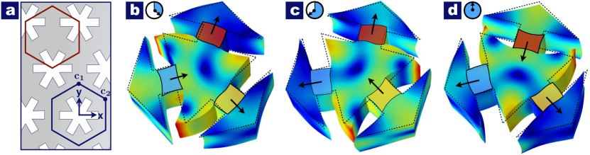
Figure 5: Eigenmodes of the silicon snowflake phononic crystal. (a) Different choices of the unit-cell: While the blue cell will nicely illustrate the motion of the snowflake itself (cf. Figure 1c), the red one rather emphasizes the motion of the links connecting the triangles (cf. b-d). (b-d) Displacement field of the same eigenmode shown in Figure 1c of the main text ($m_{s}=-1$, $\tau=-1$). Subsequent snapshots are taken after one third of a period (cf. the clocks), where the arrow indicates the current direction of the links’ velocities. Notice that the quasi-angular momentum about the center of the unit cell is $m_{1}=1$ (anti-clockwise rotation).

Appendix B Explanation of the essential degeneracies and symmetries of the pseudospin eigenstates

Here, we discuss the symmetries of the normal modes $\boldsymbol{\psi}_{m_{s},\tau}$ of the snowflake crystal at the high-symmetry points. Thereby we also explain the appearance of the essential degeneracies underpinning the robust Dirac cones, and explain how to identify a pseudospin eigenstate from the FEM simulation of a strip.

We consider a generic mode $\boldsymbol{\psi}(\mathbf{x},z)$ with quasimomentum $\mathbf{k}$,

$$\hat{T}(\boldsymbol{a})\boldsymbol{\psi}(\mathbf{x},z)=\boldsymbol{\psi}(\mathbf{x}-\boldsymbol{a},z)=e^{-i\mathbf{k}\cdot\boldsymbol{a}}\boldsymbol{\psi}(\mathbf{x},z)$$

where $\hat{T}(\boldsymbol{a})$ is a translation by a lattice vector $\boldsymbol{a}$. As usual we can use the Bloch ansatz

$$\boldsymbol{\psi}(\mathbf{x},z)=e^{i\mathbf{k}\cdot\mathbf{x}}\boldsymbol{\phi}(\mathbf{x},z),$$ (6)

where $\boldsymbol{\phi}(\mathbf{x},z)$ is periodic under discrete translations, $\boldsymbol{\phi}(\mathbf{x},z)=\boldsymbol{\phi}(\mathbf{x}-\boldsymbol{a},z)$. We choose the center of the snowflake as the origin of the coordinates, see Figure 5a. By applying a rotation by a angle $\theta$ about the $z$-axis, we find

$$\hat{R}(\theta)_{z}[\boldsymbol{\psi}(\mathbf{x},z)] = R(\theta)_{z}\boldsymbol{\psi}(R(-\theta)\mathbf{x},z)$$ (7)

$$= e^{i\mathbf{k}\cdot R(-\theta)\mathbf{x}}R(\theta)_{z}\boldsymbol{\phi}(R(-\theta)\mathbf{x},z)$$

$$= e^{iR(\theta)\mathbf{k}\cdot\mathbf{x}}R(\theta)_{z}\boldsymbol{\phi}(R(-\theta)\mathbf{x},z)$$

where

$$R(\theta)_{z}=\begin{pmatrix}R(\theta)&0\\ 0&1\end{pmatrix},\quad R(\theta)=\begin{pmatrix}\cos\theta&-\sin\theta\\ \sin\theta&\cos\theta\end{pmatrix}.$$ (8)

We note that $\hat{R}(\theta)_{z}[\boldsymbol{\psi}(\mathbf{x})]$ has a quasimomentum $\mathbf{k}^{\prime}=R(\theta)\mathbf{k}$ rotated by $\theta$. For a triangular lattice, the high-symmetry points $\mathbf{K}$, $\mathbf{K}^{\prime}$, and $\boldsymbol{\Gamma}$ have the peculiarity to be invariant under ${\cal C}_{3}$ rotations. For example, $R(2\pi/3)\mathbf{K}=\mathbf{K}+\mathbf{b}_{1}$ where $\mathbf{b}_{1}$ is a basis vector of the reciprocal lattice. Thus, applying the rotation $\hat{R}(2\pi/3)_{z}$ to a state with quasimomentum $\mathbf{k}=\mathbf{K}$, see Eq. (7), we find another state with the same quasimomentum,

$$\hat{R}(2\pi/3)_{z}[\boldsymbol{\psi}(\mathbf{x},z)]=e^{i\mathbf{K}\cdot\mathbf{x}}\boldsymbol{\phi}^{\prime}(\mathbf{x},z)$$

where

$$\boldsymbol{\phi}^{\prime}(\mathbf{x},z)=e^{i\mathbf{b_{1}\cdot\mathbf{x}}}R(2\pi/3)_{z}\boldsymbol{\phi}(R(-2\pi/3)\mathbf{x},z)$$

is invariant under $2D$ discrete translations, $\boldsymbol{\phi}^{\prime}(\mathbf{x}+\boldsymbol{a},z)=\boldsymbol{\phi^{\prime}}(\mathbf{x},z)$. In other words, $\hat{R}(2\pi/3)_{z}$ (and more in general any ${\cal C}_{3}$ rotation) commutes with the projector $\hat{P}_{\mathbf{K}}$ onto the states with quasimomentum $\mathbf{K}$. The same holds for $\mathbf{K}^{\prime}$, and $\boldsymbol{\Gamma}$. Thus, for each high-symmetry point $\mathbf{k}=\mathbf{K},\mathbf{K}^{\prime},$ and $\boldsymbol{\Gamma}$, it is possible to find a basis of eigenstates of the ${\cal C}_{3}$ rotations spanning the sub-Hilbert space of states with that particular quasimomentum. If the crystal has the $2D$ discrete translational invariance and the ${\cal C}_{3}$ symmetry, such a basis can be chosen to be eigenstates of the Hamiltonian.

In the following, we denote a common eigenstate of the ${\cal C}_{3}$ rotations and the translations by $\boldsymbol{\psi}_{m_{s},\tau}(\mathbf{x})$ where $\tau$ indicates the valley ($\tau=1$ for $\mathbf{k}=\mathbf{K}$ and $\tau=-1$ for $\mathbf{k}=\mathbf{K}^{\prime}$ ) and $m_{s}$ the quasi-angular momentum,

$$\hat{R}(2\pi/3)_{z}[\boldsymbol{\psi}_{m_{s},\tau}(\mathbf{x},z)]=e^{-im_{s}2\pi/3}\boldsymbol{\psi}_{m_{s,\tau}}(\mathbf{x},z).$$

From Eq. (7), we see that in terms of the corresponding translational invariant field $\boldsymbol{\phi}_{m_{s},\tau}(\mathbf{x},z)$ we have

$$e^{i\mathbf{\tau b_{1}\cdot\mathbf{x}}}R(2\pi/3)_{z}\boldsymbol{\phi}_{m_{s},\tau}(R(-2\pi/3)\mathbf{x},z)\\ =e^{-im_{s}2\pi/3}\boldsymbol{\phi}_{m_{s},\tau}(\mathbf{x},z)$$ (9)

Next, we show that the eigenstates with non-zero quasi-angular momentum $m_{s}=\pm 1$ at the valleys $\tau=\pm 1$ can be organized in quadruplets which are degenerate if the Hamiltonian has time-reversal symmetry ${\cal T}$ and the full ${\cal C}_{6}$ symmetry. We denote the members of the quadruplet $\boldsymbol{\psi}_{m_{s},\tau}(\mathbf{x})$. Starting from an arbitrary state with $m_{s}=1$ or $m_{s}=-1$, the remaining three members of the quadruplet are (by definition) obtained by applying the time-reversal symmetry ${\cal T}$ and $\hat{R}(\pi)_{z}$ (a rotation by $\pi$ about the $z$-axis),

$$\boldsymbol{\psi}_{-m_{s},-\tau}(\mathbf{x},z) = {\cal T}\boldsymbol{\psi}_{m_{s},\tau}(\mathbf{x},z),$$

$$\boldsymbol{\psi}_{m_{s},-\tau}(\mathbf{x},z) = \hat{R}(\pi)_{z}\boldsymbol{\psi}_{m_{s},\tau}(\mathbf{x},z),$$

$$\boldsymbol{\psi}_{-m_{s},\tau}(\mathbf{x},z) = {\cal T}\hat{R}(\pi)_{z}\boldsymbol{\psi}_{m_{s},\tau}(\mathbf{x},z).$$

where ${\cal T}\boldsymbol{\psi}_{m_{s},\tau}(\mathbf{x},z)=\boldsymbol{\psi}_{m_{s},\tau}^{*}(\mathbf{x},z).$ It is straightforward to explicitly check that the states $\boldsymbol{\psi}_{-m_{s},-\tau}(\mathbf{x},z)$, $\boldsymbol{\psi}_{m_{s},-\tau}(\mathbf{x},z)$, and $\boldsymbol{\psi}_{-m_{s},\tau}(\mathbf{x},z)$ as obtained via the above definitions from $\boldsymbol{\psi}_{m_{s},\tau}(\mathbf{x})$ are indeed eigenstates of the ${\cal C}_{3}$ rotations and the discrete translations with the appropriate eigenvalues. For the ${\cal C}_{3}$ rotation we have to show that if Eq. (9) is assumed to hold for a specific choice of $m_{s}$ and $\tau$, it will hold also for the remaining combinations of $m_{s}$ and $\tau$.

Next we discuss the behavior of the states $\boldsymbol{\psi}_{m_{s},\tau}(\mathbf{x})$ under ${\cal C}_{3}$ rotations about the center of the downwards and upwards triangles, cf. Figure 5a,

$$\mathbf{c}_{1}=\left(0,\frac{a}{\sqrt{3}}\right),\quad\mathbf{c}_{2}=\left(\frac{a}{2},\frac{a}{2\sqrt{3}}\right),$$

respectively. We note that these points lie at the corners of the Wigner-Seitz cell around the ${\cal C}_{6}$ rotocenter (in this case the snowflake center). Thus, as in any ${\cal C}_{6}$ symmetric triangular lattice, they are threefold rotocenters. The states $\boldsymbol{\psi}_{m_{s},\tau}(\mathbf{x},z)$ are also eigenstates of the ${\cal C}_{3}$ rotations about $\mathbf{c}_{1}$ and $\mathbf{c}_{2}$ (or about any other point belonging to the corresponding Bravais lattices) with quasi-angular momentum

$$m_{{\rm 1}} = (m_{{\rm s}}+\tau+1){\rm mod}3-1,$$

$$m_{{\rm 2}} = (m_{{\rm s}}-\tau+1){\rm mod}3-1,$$ (10)

respectively. Here, we use the definition of the function $(n){\rm mod}3$ where $(-1){\rm mod}3=2$. It is easy to verify the above statement by applying the rotation $\hat{R}(2\pi/3)_{\mathbf{c}_{i},z}$ about the point $\mathbf{c}_{i}$ to the normal modes $\boldsymbol{\psi}_{m_{s},\tau}(\mathbf{x},z)$,

$$\hat{R}(2\pi/3)_{\mathbf{c}_{i},z}\boldsymbol{\psi}_{m_{s},\tau}(\mathbf{x},z)\\ =\hat{T}(\mathbf{c}_{i})\hat{R}(2\pi/3)_{,z}\hat{T}(-\mathbf{c}_{i})\boldsymbol{\psi}_{m_{s},\tau}(\mathbf{x},z)\\ =e^{-i(m_{s}+\tau\mathbf{b_{1}}\cdot\mathbf{c}_{i})2\pi/3}\boldsymbol{\psi}_{m_{s},\tau}(\mathbf{x},z).$$

Taking into account that $\mathbf{b_{1}}\cdot\mathbf{c}_{1}=2\pi/3$ and $\mathbf{b_{1}}\cdot\mathbf{c}_{2}=-2\pi/3$ we arrive to Eq. (10). Since $\boldsymbol{\psi}_{m_{s},\tau}(\mathbf{x},z)$ are simultaneous eigenvectors of the ${\cal C}_{3}$ rotations about all three inequivalent threefold rotocenters of the crystal (the origin, $\mathbf{c_{1}}$ and $\mathbf{c_{2}}$), the time-averaged squared displacement field $|\boldsymbol{\psi}_{m_{s},\tau}(\mathbf{x},z)|^{2}$ is invariant under all these symmetry transformations, cf. Figure 1b of the main text. We note that for $m_{s}\tau=1$ ($m_{s}\tau=-1$), the quasi-angular momentum about the center of the downward (upwards) triangles $\mathbf{c}_{1}$ ($\mathbf{c}_{2}$ ) is finite, $|m_{1}|=1$ ($|m_{2}|=1$), corresponding to a vortex configuration. Thus, the wavefunction has nodes at these points, cf. Figure 1b of the main text.

We note that a generic pseudospin eigenstate, e. g. the zero Landau level, is the product of a smooth function and the normal mode $\boldsymbol{\psi}_{m_{s},\tau}(\mathbf{x},z)$. Thus, it will show the same displacement pattern at the lattice scale, cf. Fig 3d of the main text. Consequently, the pseudo-spin can be immediately read off from a FEM simulation of a strip (where the valley is known) just by observing the location of the nodes of $|\boldsymbol{\psi}_{m_{s},\tau}(\mathbf{x},z)|^{2}$ .

Appendix C Derivation of the Dirac equation in the presence of the $\boldsymbol{C}_{6}$ symmetry

Here, we derive the Dirac Hamiltonian for the case where the ${\cal C}_{6}$ symmetry is preserved [Equation (1) of the main text with $m=0$ and $\mathbf{A}=0$]. In each valley ($\tau=\pm 1$), we project the Hamiltonian onto the states $\boldsymbol{\psi}_{\mathbf{p},1,\tau}(\mathbf{x},z)=e^{i\mathbf{p}\cdot\mathbf{x}}\boldsymbol{\psi}_{1,\tau}(\mathbf{x},z)$ and $\boldsymbol{\psi}_{\mathbf{p},-1,\tau}(\mathbf{x},z)=e^{i\mathbf{p}\cdot\mathbf{x}}\boldsymbol{\psi}_{-1,\tau}(\mathbf{x},z)$, where the quasimomentum $\mathbf{p}$ counted off from the symmetry point is assumed to be small. For each $\mathbf{p}$ we define the Pauli matrices according to

$$\hat{\sigma}_{z,\mathbf{p}}=|\boldsymbol{\psi}_{\mathbf{p},-1,\tau}\rangle\langle\boldsymbol{\psi}_{\mathbf{p},-1,\tau}|-|\boldsymbol{\psi}_{\mathbf{p},1,\tau}\rangle\langle\boldsymbol{\psi}_{\mathbf{p},1,\tau}|.$$

From this definition (assuming the usual commutation relations for the Pauli matrices) we also have

$$\hat{\sigma}_{+,\mathbf{p}}=(\hat{\sigma}_{x,\mathbf{p}}+i\hat{\sigma}_{y,\mathbf{p}})/2=|\boldsymbol{\psi}_{\mathbf{p},-1,\tau}\rangle\langle\boldsymbol{\psi}_{\mathbf{p},1,\tau}|.$$

From the band structure calculated by the FEM simulations (without the pseudomagnetic fields) we see that the eigenenergies are linear in $|\mathbf{p}|$ close to the relevant symmetry point (they form a cone). Thus, the Hamiltonian should be, to first approximation, linear in $\mathbf{p}$. Taking into account that $\boldsymbol{\psi}_{\mathbf{p},-1,\tau}(\mathbf{x},z)={\cal T}\hat{R}(\pi)_{z}\boldsymbol{\psi}_{\mathbf{p},1,\tau}(\mathbf{x},z)$ and that ${\cal T}\hat{R}(\pi)_{z}$ is a symmetry, a mass term (proportional to $\hat{\sigma}_{z,\mathbf{p}}$ ) is forbidden and the most general Hamiltonian which is linear in $\mathbf{p}$ has the form

$$\hat{H}=\bar{E}+\sum_{\mathbf{p}}\mathbf{v}\cdot\mathbf{p}\hat{\sigma}_{+,\mathbf{p}}+h.c.$$ (11)

where $\bar{E}$ is the degenerate energy of the normal modes $\boldsymbol{\psi}_{m_{s},\tau}(\mathbf{x},z)$. Under the rotation $\hat{R}(2\pi/3)_{z}$ we have

$$\hat{R}(2\pi/3)_{z}\hat{H}\hat{R}(-2\pi/3)_{z}\\ =\sum_{\mathbf{p}}\mathbf{v}\cdot\mathbf{p}\hat{R}(2\pi/3)_{z}\hat{\sigma}_{+,\mathbf{p}}\hat{R}(-2\pi/3)_{z}+h.c.\\ =\sum_{\mathbf{p}}\mathbf{v}\cdot\mathbf{p}e^{-i2\pi/3}\hat{\sigma}_{+,R(2\pi/3)\mathbf{p}}+h.c.\\ =\sum_{\mathbf{p}}(R(2\pi/3)\mathbf{v})\cdot\mathbf{p}e^{-i2\pi/3}\hat{\sigma}_{+,\mathbf{p}}+h.c.$$

Since the Hamiltonian is invariant under ${\cal C}_{3}$ rotations we must have

$$R(2\pi/3)\mathbf{v}=e^{i2\pi/3}\mathbf{v}.$$

From Eq. (8), we find $\mathbf{v}=v(1,-i)$ where $v$ is the slope of the cones. By plugging into Eq. (11) and projecting onto a single quasimomentum we obtain the Dirac equation (1) of the main text [for $m=0$ and $\mathbf{A}=0$].

Appendix D Details of the numerical calculations of the pseudomagnetic fields

In this section we provide additional details about the numerical calculations performed with the COMSOL finite-element solver, thereby guiding through the computation of the movements of the Dirac cones in reciprocal space and the construction of the resulting pseudo magnetic field for phonons in a strip configuration. In all calculations the material is assumed to be silicon (Si) with Young’s modulus of $170\,\text{GPa}$, mass density $2329\,\text{kg/m}^{3}$ and Poisson’s ratio $0.28$.

Breaking the 3-fold rotational symmetry ($\mathcal{C}_{3}$-symmetry) of the snowflake geometry but maintaining its inversion symmetry ($\mathcal{C}_{2}$-symmetry), displaces the Dirac cones from the high symmetry points ${\bf K}$ and ${\bf K}^{\prime}$, but does not gap the system (cf. Figure 2c of the main text). This effect is depicted in Figure 6, which shows the motion of the Dirac cones, as an effect of the broken $\mathcal{C}_{3}$-symmetry. Thereby the radius of the horizontally orientated snowflake arm is varied by $\delta r_{1}$ ($r_{1}=\bar{r}+\delta r_{1}$), which displaces the Dirac cones in the $k_{x}$-direction. Generally this would also shift the Dirac cone’s energy. In order to avoid that, the remaining two snowflake arms are varied equivalently by $\delta r_{2}=\delta r_{3}$ in such a way that the average radius is kept fixed at $\bar{r}=(r_{1}+r_{2}+r_{3})/3=180\,\text{nm}$ (i.e $\delta r_{1}+\delta r_{2}+\delta r_{3}=0$).

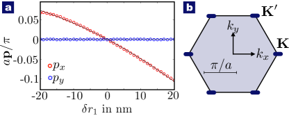
Figure 6: Displacement of the Dirac cones in reciprocal space due to a broken $\mathcal{C}_{3}$-symmetry (cf. Figure 2a of the main text). Here the snowflakes arm lengths $r_{i}=\bar{r}+\delta r_{i}$ are changed with $\delta r_{1}\neq\delta r_{2}=\delta r_{3}$, while $\delta r_{1}+\delta r_{2}+\delta r_{3}=0$ in order to keep the average radius constant at $\bar{r}=180\,\text{nm}$. (a) depicts the shift of the Dirac cone ${\bf p}$ at ${\bf k={\bf K^{\prime}}}$ ($\tau=\text{-}1$ valley) computed by the COMSOL finite element solver for different arm length $\delta r_{1}$ (red and blue circles). For the other valley $(\tau=1$) the cones move in the opposite direction, which builds the foundation of a pseudo magnetic field for phonons that does not break the time-reversal symmetry. The data can be very well fitted by a parabola (solid black lines). (b) Overview of the Brillouin zone, with the blue bars indicating the range of the Dirac cones position that can be achieved by a variation of the snowflake arm length by $\delta r_{1}=[-20;+20]\text{nm}$.

To engineer a constant pseudo magnetic field in a strip configuration, that is infinitely extended in the x-direction, the snowflakes need to be designed properly: The B-field is given by $B_{z}=\partial A_{y}/\partial x-\partial A_{x}/\partial y$, whereas the vector potential for a given valley is directly related to the shift of the Dirac cones ${\bf A}={\bf p}$. As the strip is periodically extended in the x-direction the vector field is not allowed to vary along this direction (i.e.$\partial A_{y}/\partial x=0$), while $A_{x}$ must depend linearly on the vertical position $y$ (i.e. $\partial A_{x}/\partial y=const.$), in order to have a constant magnetic field (cf. Figure 7a). Using the relation between the shift of the Dirac cones and the variation of the radii (quadratic fit in Figure 6a), the radii of the snowflakes can be calculated in dependence of their position in the strip (cf. Figure 7b). In addition to that, we want to engineer smooth boundaries by opening a mass gap, which is done by breaking two-fold rotational symmetry at the edges of the sample. This can be achieved by displacing one of the snowflake arms by $\Delta$ (cf. Figure 2a of the main text), with $\Delta=0$ in the bulk region while it smoothly increases in the vicinity of the sample’s edge (cf. Figure 7c).

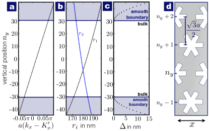
Figure 7: Details about the strip configuration (cf. Figure 3 of the main text ). (a) depicts the displacement of the Dirac cone in the $\tau=-1$ valley ($k_{x}=K_{x}^{\prime}=2\pi/3a$) as a function of the vertical position $n_{y}$ in the strip, which forms the basis of a pseudo-magnetic field for phonons. Those shifts arise from the broken $\mathcal{C}_{3}$-symmetry, due to the variation of the snowflakes’ radii $r_{1}$ and $r_{2}=r_{3}$ (cf. Figure 2a of the main text). The exact values of $r_{1}$ and $r_{2}$ in dependence of the position $n_{y}$ can be seen in (b). Displacing one of the snowflake arms by $\Delta$ (cf. Figure 2b) locally breaks the $\mathcal{C}_{2}$-symmetry, which forms smooth boundaries. In (c) the displacement $\Delta$ is depicted in dependence of $n_{y}$. (d) A small fraction of the stipe’s unit cell. The whole strip comprises 61 snowflakes in the bulk area $(|n_{y}|\leq 30)$ and additional 30 snowflakes to form the smooth boundaries ($30<|n_{y}|\leq$45). As it is infinitely extended in the x-direction a Floquet periodic boundary condition is implemented at the left and right boundaries, whereas the upper and lower boundaries are kept fixed (${\bf u}=0$).

Appendix E Edge States at the Physical Boundary

In the Figure 8, we investigate the intrinsic edge states that appear at the physical edge of the strip and that will be present even in the absence of pseudo-magnetic fields. The relevant bands are highlighted as colored lines in the band structure of the strip, see panel a. The corresponding displacement fields are shown in panel b. Note that the edge states are defined only on a finite portion of the Brillouin zone (where the bands are plotted as dashed lines) and smoothly transform into bulk modes in the remaining quasimomentum range.

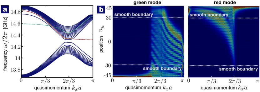
Figure 8: Intrinsic edge modes at the physical boundaries. (a) Band structure of the strip configuration discussed in the main text and in Section D. The bands highlighted in green and red feature modes that are highly confined at the physical boundary of the sample (dashed parts). (b) Displacement field of the red and green mode. Due to the small slope of their bands for corresponding quasimomenta, the velocities become zero. Therefore, the edge states are stationary and do not show any transport properties.

Appendix F Tight Binding Model on the Kagome lattice

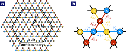
Figure 9: (a) Scheme of the Kagome tight binding lattice on a hexagon. The solid triangles indicate the unit cells, whereas the dashed lines illustrate the nearest neighbor coupling to different unit cells. The three different colors illustrate the different sublattice sites. The red hexagonal line separates the bulk area (inner part) from the boundary area (outer part) (b) Zoom into the lattice, depicting one unit cell and its six neighboring sites. Within one unit cell mechanical excitations can hop from one site to another with the internal hopping rates $J_{AB}^{(i)}$, $J_{BA}^{(i)}$ and $J_{CA}^{(i)}$, whereas external hopping rates out of one unit cell are labeled with $J_{AB}^{(e)}$, $J_{BA}^{(e)}$ and $J_{CA}^{(e)}$. Note that internal and external hopping rates are equal if the $\mathcal{C}_{2}$-symmetry is maintained.

For the transport calculations, we have modeled the hexagonal snowflake crystal by a tight-binding Hamiltonian on a Kagome lattice, which is the lattice that describes the links between neighboring triangles, whose motion represents the relevant sound waves for the particular triple of bands that we choose to consider. The Kagome lattice Hamiltonian reads,

$$\hat{H}=\sum_{\mathbf{j}}(\bar{E}+\delta E)\hat{a}_{\mathbf{j}}^{\dagger}\hat{a}_{\mathbf{j}}+\sum_{\langle\mathbf{j},\mathbf{j}^{\prime}\rangle}J_{{\rm\mathbf{j,j^{\prime}}}}\hat{a}_{\mathbf{j}}^{\dagger}\hat{a}_{\mathbf{j^{\prime}}}.$$ (12)

Here, $\mathbf{j}$ is a multi-index, $\mathbf{j}=(j_{1},j_{2},s)$ where $j_{1/2}$ label the unit cell, and $s=A,B,C$ the sublattice, see Figure 9a. As usual, $\langle\mathbf{j},\mathbf{j}^{\prime}\rangle$ indicates the sum over the nearest neighbors. The hopping matrix $K_{{\rm\mathbf{j,j^{\prime}}}}$ is symmetric and its matrix elements are chosen to reproduce the same Dirac equation that would effectively describe our patterned snowflake crystal. The energy $\bar{E}$ is the eigenenergy of the states $\boldsymbol{\psi}_{m_{s},\tau}$ for the rotationally symmetric crystal (see main text) while $\delta E$ cancel out a renormalization of the energy by the hopping terms.

In the main text and in the Appendix D, we have shown how the FEM simulations can be mapped onto the effective Dirac Hamiltonian Equation (1) of the main text. Here, we show how the tight-binding model Eq. (12) can be mapped onto the same effective Hamiltonian. We first consider the simple case where the invariance under discrete translations and the ${\cal C}_{6}$ symmetry are not broken corresponding to $m=0$ and $\mathbf{A}=0$. In this case, all (nearest-neighbor) hopping rates must be equal $K_{{\rm\mathbf{j,j^{\prime}}}}=K.$ One can easily calculate the equivalent first-quantized Hamiltonian

$$h(\mathbf{k})=\begin{pmatrix}\bar{E}+\delta E&J(1+e^{-i\mathbf{k}\cdot\boldsymbol{a}_{1}})&J(1+e^{i\mathbf{k}\cdot\boldsymbol{a}_{3}})\\ J(1+e^{i\mathbf{k}\cdot\boldsymbol{a}_{1}})&\bar{E}+\delta E&J(1+e^{-i\mathbf{k}\cdot\boldsymbol{a}_{2}})\\ J(1+e^{-i\mathbf{k}\cdot\boldsymbol{a}_{3}})&J(1+e^{i\mathbf{k}\cdot\boldsymbol{a}_{2}})&\bar{E}+\delta E\end{pmatrix},$$

where $\boldsymbol{a}_{1}=(a,0),$ $\boldsymbol{a}_{2}=a(-1,\sqrt{3})/2,$ and $\boldsymbol{a}_{3}=a(-1,-\sqrt{3})/2$. By expanding around $\mathbf{k}=\mathbf{K}$ or $\mathbf{k}=\mathbf{K}^{\prime}$ and projecting onto the states $|m_{1}=0,\tau\rangle=(1,1,1)/\sqrt{3}$ and $|m_{1}=-\tau,\tau\rangle=(1,e^{-i2\pi\tau/3},e^{i2\pi\tau/3})/\sqrt{3}$ ($m_{1}$ is the quasimomentum about the center of the downwards triangles) we find the Dirac Hamiltonian (1) of the main text with $m=0,$ $\mathbf{A}=0,$ and $v=\sqrt{3}aK/2$. The energy at the tip of the cones is $\bar{E}$ if $\delta E=-J$.

Next, we break the ${\cal C}_{6}$ symmetry but preserve the translational symmetry such that the mass $m$ and the gauge $\mathbf{A}$ fields are constants. In this case, there are six different hopping rates. Three of them describe the hopping within the same (to a different) unit cell $J_{\mathbf{j},\mathbf{j^{\prime}}}=J_{s,s^{\prime}}^{(i)}=J+\delta J_{s,s^{\prime}}^{(i)}$ ($J_{\mathbf{j},\mathbf{j^{\prime}}}=J_{s,s^{\prime}}^{(e)}=J+\delta J_{s,s^{\prime}}^{(e)}$) where $s\neq s^{\prime}$ and $j_{x/y}=j_{x/y}^{\prime}$ ($j_{x/y}\neq j_{x/y}^{\prime}$). The resulting first-quantized Hamiltonian reads

$$h(\mathbf{k})=\begin{pmatrix}\bar{E}+\delta E&h_{AB}(\mathbf{k}\cdot\boldsymbol{a}_{1})&h_{CA}^{*}(\mathbf{k}\cdot\boldsymbol{a}_{3})\\ h_{AB}^{*}(\mathbf{k}\cdot\boldsymbol{a}_{1})&\bar{E}+\delta E&h_{BC}(\mathbf{k}\cdot\boldsymbol{a}_{2})\\ h_{CA}(\mathbf{k}\cdot\boldsymbol{a}_{3})&h_{BC}^{*}(\mathbf{k}\cdot\boldsymbol{a}_{2})&\bar{E}+\delta E\end{pmatrix},$$

where $h_{ss^{\prime}}(\mathbf{x)}\equiv J_{ss^{\prime}}^{(i)}+J_{ss^{\prime}}^{(e)}e^{-i\mathbf{x}}.$ Since we are interested in the case where the ${\cal C}_{6}$ symmetry is broken only weakly, we assume $\delta J_{s,s^{\prime}}^{(i/e)}\ll J$. Up to leading order in $\delta J_{s,s^{\prime}}^{(i/e)}$ this correspond to the the Dirac Hamiltonian (1) of the main text with

$$\mathbf{A} \approx -\tau[(J_{AB}^{(e)}+J_{AB}^{(i)})\mathbf{e}_{1}+(J_{BC}^{(e)}+J_{BC}^{(i)})\mathbf{e}_{2}$$ (13)

$$\quad\,\,+(J_{CA}^{(e)}+J_{CA}^{(i)})\mathbf{e}_{3}]/v,$$

$$m \approx (J_{AB}^{(e)}+J_{BC}^{(e)}+J_{CA}^{(e)}-J_{AB}^{(i)}-J_{BC}^{(i)}-J_{CA}^{(i)})/2,\,\,\,\,\,\,\,\,\,\,\,\,$$ (14)

$$\delta E \approx- (J_{AB}^{(i)}+J_{BC}^{(i)}+J_{CA}^{(i)}+J_{AB}^{(e)}+J_{BC}^{(e)}+J_{CA}^{(e)})/6,\,\,\,\,\,\,\,\,\,\,\,$$ (15)

where the vectors $\mathbf{e}_{j}$ are defined in the main text.

With the help of the relations (13,14,15) we can simulate the Dirac Hamiltonian (1) of the main text with the desired constant pseudo-magnetic field (in the symmetric gauge $\mathbf{A}=\tau B(y,-x,0)/2$) and mass profile. To simulate the disorder we add and additional random energy shift $\Omega_{\mathbf{j}}$ equally distributed on the interval $-\Delta\Omega/2<\Omega_{\mathbf{j}}<\Delta\Omega/2.$ A finite decay rate of the phonons (necessary to reach a steady state), is described within the standard input/output formalism GerryKnight . In the simulations with the drains, the decay rate is increase smoothly in the regions of the drains (in order to avoid introducing any additional backscattering).

Appendix G Possible Implementations

Here, we provide a few more comments regarding the optomechanical excitation and read out of helical waves. In the simplest approach without a cavity, one could illuminate the structure from above by tightly focussed laser beams, exerting radiation pressure directly. A rough estimate of the force, for a laser power of $1\,\text{mW}$, indicates that (out-of-plane) vibrational amplitudes of the order of $10$fm might be achieved. In this estimate, we have adopted the simplest possible approach, treating the triangle as an oscillator with a frequency of order $2\pi\cdot 14{\rm GHz}$ and a decay rate ($2{\rm GHz}$) set by the scale of the bandwidth of the Kagome bands. A more detailed analysis would be needed to extract the excitation efficiency for the particular vibrational modes of interest, which formed the basis of our discussion in the main text.

However, a much more efficient approach is available, involving optical cavities. A structure scaled up by a factor of $X=10$ (resulting in frequencies lower by $X$) can host defect-mode nano cavities embedded in the triangles itself, cf. Figure 10. For any such optical cavity, a circulating light with a modulated intensity will give rise (via radiation pressure and photoelastic forces) to periodic cycles of expansion and contraction of the structure. This type of motion (when the right frequency is selected) clearly overlaps with the vibrational modes that are relevant for our proposal, cf. Fig. 1d–f of the main text. We note that the light intensity is enhanced by the cavity’s finesse (usually at least $\gtrsim 100$), thereby increasing the amplitude of the vibrations. As the thermal motion decreases with the factor $1/\sqrt{X}$, it is easily possible to overcome the thermal motion at room temperature. In addition, during the measurements one can average out the noise and provide a clear signal of the excited sound waves traveling through the structure, regardless of thermal fluctuations.

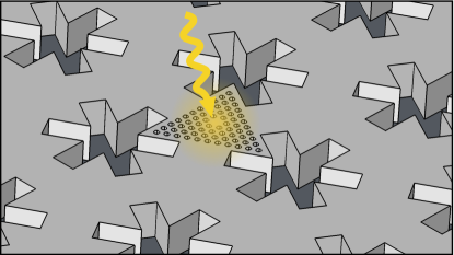
Figure 10: Schematic picture of a scaled up snowflake array with one triangle hosting a defect-mode nano cavity. Impinging light is enhanced by the cavity’s finesse thereby launching mechanical excitations via the optomechanical interaction.

References

- (1) Lisa M. Nash, Dustin Kleckner, Alismari Read, Vincenzo Vitelli, Ari M. Turner, and William T. M. Irvine. Topological mechanics of gyroscopic metamaterials. Proceedings of the National Academy of Sciences, 112(47):14495–14500, 2015.
- (2) Roman Süsstrunk and Sebastian D. Huber. Observation of phononic helical edge states in a mechanical topological insulator. Science, 349(6243):47–50, 2015.
- (3) C. L. Kane and T. C. Lubensky. Topological boundary modes in isostatic lattices. Nature Phys., 10(1):39–45, 2013.
- (4) Jayson Paulose, Bryan Gin-ge Chen, and Vincenzo Vitelli. Topological modes bound to dislocations in mechanical metamaterials. Nature Phys., 11(2):153–156, February 2015.
- (5) Meng Xiao, Guancong Ma, Zhiyu Yang, Ping Sheng, Z. Q. Zhang, and C. T. Chan. Geometric phase and band inversion in periodic acoustic systems. Nat Phys, 11(3):240–244, March 2015.
- (6) C. He, X. Ni, H. Ge, X.-C. Sun, Y.-B. Chen, M.-H. Lu, X.-P. Liu, L. Feng, and Y.-F. Chen. Acoustic topological insulator and robust one-way sound transport. arXiv:1512.03273, December 2015.
- (7) D. Zeb Rocklin, Shangnan Zhou, Kai Sun, and Xiaoming Mao. Transformable topological mechanical metamaterials. arXiv:1510.06389, 2015.
- (8) Bryan Gin-ge Chen, Nitin Upadhyaya, and Vincenzo Vitelli. Nonlinear conduction via solitons in a topological mechanical insulator. Proceedings of the National Academy of Sciences, 111(36):13004–13009, 2014.
- (9) Zhaoju Yang, Fei Gao, Xihang Shi, Xiao Lin, Zhen Gao, Yidong Chong, and Baile Zhang. Topological acoustics. Phys. Rev. Lett., 114:114301, Mar 2015.
- (10) Alexander B. Khanikaev, Romain Fleury, S. Hossein Mousavi, and Andrea Alu. Topologically robust sound propagation in an angular-momentum-biased graphene-like resonator lattice. Nat Commun, 6:8260, October 2015.
- (11) Toshikaze Kariyado and Yasuhiro Hatsugai. Manipulation of dirac cones in mechanical graphene. Scientific Reports, 5:18107–, December 2015.
- (12) Pai Wang, Ling Lu, and Katia Bertoldi. Topological phononic crystals with one-way elastic edge waves. Phys. Rev. Lett., 115:104302, Sep 2015.
- (13) Raj Kumar Pal, Marshall Schaeffer, and Massimo Ruzzene. Helical edge states and topological phase transitions in phononic systems using bi-layered lattices. Journal of Applied Physics, 119(8), 2016.
- (14) Romain Fleury, Alexander B Khanikaev, and Andrea Alu. Floquet topological insulators for sound. Nat Commun, 7:11744, June 2016.
- (15) Jun Mei, Ze-Guo Chen, and Ying Wu. Pseudo-time-reversal symmetry and topological edge states in two-dimensional acoustic crystals. arXiv:1606.02944, (2016).
- (16) Ze-Guo Chen and Ying Wu. Tunable topological phononic crystals. Phys. Rev. Applied, 5:054021, May 2016.
- (17) D. Zeb Rocklin, Bryan Gin-ge Chen, Martin Falk, Vincenzo Vitelli, and T. C. Lubensky. Mechanical weyl modes in topological maxwell lattices. Phys. Rev. Lett., 116:135503, Apr 2016.
- (18) Daniel M. Sussman, Olaf Stenull, and T. C. Lubensky. Topological boundary modes in jammed matter. Soft Matter, 12:6079–6087, 2016.
- (19) Emil Prodan and Camelia Prodan. Topological phonon modes and their role in dynamic instability of microtubules. Phys. Rev. Lett., 103:248101, Dec 2009.
- (20) Jiuyang Lu, Chunyin Qiu, Manzhu Ke, and Zhengyou Liu. Valley vortex states in sonic crystals. Phys. Rev. Lett., 116:093901, Feb 2016.
- (21) Roman Süsstrunk and Sebastian D. Huber. Classification of topological phonons in linear mechanical metamaterials. arXiv:1604.01033, (2016).
- (22) V. Peano, C. Brendel, M. Schmidt, and F. Marquardt. Topological phases of sound and light. Phys. Rev. X, 5:031011, Jul 2015.
- (23) S. Hossein Mousavi, Alexander B. Khanikaev, and Zheng Wang. Topologically protected elastic waves in phononic metamaterials. Nat Commun, 6:8682, November 2015.
- (24) Amir H. Safavi-Naeini, Jeff T. Hill, Seán Meenehan, Jasper Chan, Simon Gröblacher, and Oskar Painter. Two-dimensional phononic-photonic band gap optomechanical crystal cavity. Phys. Rev. Lett., 112:153603, 2014.
- (25) C. L. Kane and E. J. Mele. Size, shape, and low energy electronic structure of carbon nanotubes. Phys. Rev. Lett., 78:1932–1935, Mar 1997.
- (26) J. L. Mañes. Symmetry-based approach to electron-phonon interactions in graphene. Phys. Rev. B, 76:045430, Jul 2007.
- (27) F. Guinea, M. I. Katsnelson, and A. K. Geim. Energy gaps and a zero-field quantum hall effect in graphene by strain engineering. Nat Phys, 6(1):30–33, January 2010.
- (28) N. Levy, S. A. Burke, K. L. Meaker, M. Panlasigui, A. Zettl, F. Guinea, A. H. Castro Neto, and M. F. Crommie. Strain-induced pseudo–magnetic fields greater than 300 tesla in graphene nanobubbles. Science, 329(5991):544–547, 2010.
- (29) Tony Low and F. Guinea. Strain-induced pseudomagnetic field for novel graphene electronics. Nano Letters, 10(9):3551–3554, 2010. PMID: 20715802.
- (30) Mikael C. Rechtsman, Julia M. Zeuner, Andreas Tunnermann, Stefan Nolte, Mordechai Segev, and Alexander Szameit. Strain-induced pseudomagnetic field and photonic landau levels in dielectric structures. Nat Photon, 7(2):153–158, February 2013.
- (31) Martin Maldovan. Sound and heat revolutions in phononics. Nature, 503(7475):209–217, November 2013.
- (32) Bogdan-Ioan Popa, Lucian Zigoneanu, and Steven A. Cummer. Experimental acoustic ground cloak in air. Phys. Rev. Lett., 106:253901, Jun 2011.
- (33) A. Adibi A. Khelif. Phononic Crystals: Fundamentals and Applications. Springer, 2016.
- (34) Guancong Ma and Ping Sheng. Acoustic metamaterials: From local resonances to broad horizons. Science Advances, 2(2), 2016.
- (35) A. H. Castro Neto, F. Guinea, N. M. R. Peres, K. S. Novoselov, and A. K. Geim. The electronic properties of graphene. Rev. Mod. Phys., 81:109–162, Jan 2009.
- (36) Ling Lu, John D. Joannopoulos, and Marin Soljacic. Topological photonics. Nat Photon, 8(11):821–829, November 2014.
- (37) Krishna C. Balram, Marcelo I. Davanço, Jin Dong Song, and Kartik Srinivasan. Coherent coupling between radiofrequency, optical and acoustic waves in piezo-optomechanical circuits. Nat Photon, 10(5):346–352, May 2016.
- (38) C. C. Gerry and P. L. Knight. Introductory Quantum Optics. Cambridge University Press, 2005.