Lotka-Volterra with randomly fluctuating environments: a full description

Abstract

In this note, we study the long time behavior of Lotka-Volterra systems whose coefficients vary randomly. Benaïm and Lobry established that randomly switching between two environments that are both favorable to the same species may lead to four different regimes: almost sure extinction of one of the two species, random extinction of one species or the other and persistence of both species. Our purpose here is to provide a complete description of the model. In particular, we show that any couple of environments may lead to the four different behaviours of the stochastic process depending on the jump rates.

1 Introduction

For a given set of positive parameters $\varepsilon=(a,b,c,d,\alpha,\beta),$ consider the Lotka-Volterra differential system in $\mathbb{R}_{+}^{2},$ is given by

$$\left\{\begin{array}[]{llll}x^{\prime}=\alpha x(1-ax-by)\\ y^{\prime}=\beta y(1-cx-dy)\\ (x_{0},y_{0})\in\mathbb{R}_{+}^{2}\end{array}\right.$$

We denote by $\displaystyle F_{\varepsilon}$ the associated vector field: $(x^{\prime},y^{\prime})=F_{\varepsilon}(x,y)$. Let us note already that when $a<c$ and $b<d$, the point $(1/a,0)$ attracts any path starting in $(0,+\infty)^{2}$. We say that the environment is favorable to species $x$. Similarly, when $a>c$ and $b>d$, the point $(0,1/d)$ attracts any path starting in $(0,+\infty)^{2}$. We say that the environment is favorable to species $y$. See [6] for a detailed presentation of the four generic configurations. The environment is said to be of

• Type 1: if $a<c,b<d$ (favorable to species $x$)

• Type 2: if $a>c,b>d$ (favorable to species $y$)

• Type 3: if $a>c,b<d$ (persistence)

• Type 4: if $a<c,b>d$ (extinction of species $x$ or $y$ depending on the starting point)

Consider two such systems $\varepsilon_{0}=(a_{0},b_{0},c_{0},d_{0},\alpha_{0},\beta_{0})$ and $\varepsilon_{1}=(a_{1},b_{1},c_{1},d_{1},\alpha_{1},\beta_{1})$ and introduce the random process $\{(X_{t},Y_{t},I_{t})\}$ on $\mathbb{R}\times\mathbb{R}\times\{0,1\}$ obtained by switching between these two deterministic dynamics, at rates $\lambda_{0},\lambda_{1}$. More precisely, we consider the Markov process driven by the following generator

$$Lf(z,i)=F_{i}(z)\cdot\nabla_{z}f(z,i)+\lambda_{i}(f(z,1-i)-f(z,i)),\quad(z,i)\in\mathbb{R}^{2}\times\{0,1\}.$$

Equivalently, ${(I_{t})}_{t\geq 0}$ is a Markov process on $\{0,1\}$ with jump rate $\lambda_{0}$ and $\lambda_{1}$, that is

$$\mathbb{P}(I_{t+s}=1-i|I_{t}=i,\mathcal{F}_{t})=\lambda_{i}s+o(s),$$

where $\mathcal{F}_{t}$ is the sigma field generated by $\{I_{u},u\leq t\}$. Finally, $(X_{t},Y_{t})$ is solution of

$$(X_{t}^{\prime},Y_{t}^{\prime})=F_{\varepsilon_{I_{t}}}(X_{t},Y_{t}).$$

This process on $\mathbb{R}^{2}\times\{0,1\}$ has already been studied in [3, 6]. It belongs to the class of the piecewise deterministic Markov processes introduced by Davis [4]. See also [5] for a recent review of the application areas of such processes. Let us introduce the invasion rates of species x and y defined in [3] as

$$\Lambda_{y}=\displaystyle\int\beta_{0}(1-c_{0}x)\mu(dx,0)+\int\beta_{1}(1-c_{1}x)\mu(dx,1),$$

$$\Lambda_{x}=\displaystyle\int\alpha_{0}(1-b_{0}y)\widehat{\mu}(dy,0)+\int\alpha_{1}(1-b_{1}x)\widehat{\mu}(dy,1),$$

where $\mu$ is the invariant probability measure of $(X_{t},I_{t})$ associated to equation:

$$X_{t}^{\prime}=\alpha_{I_{t}}X_{t}(1-a_{I_{t}}X_{t}),$$

and $\widehat{\mu}$ is the invariant probability measure of $(Y_{t},I_{t})$ associated to equation:

$$Y_{t}^{\prime}=\beta_{I_{t}}Y_{t}(1-d_{I_{t}}Y_{t}).$$

The meaning of $\Lambda_{y}$ is the following: when species $y$ is close to extinction, species $x$ behaves approximately as $(X^{\prime}_{t},0)=F_{\varepsilon_{I_{t}}}(X_{t},0)$ and $\Lambda_{y}$ is the growth rate of species $y$ with respect to invariant measure $\mu$ of $(X,I)$. Note that the invasion rates depend on the jump rates $(\lambda_{0},\lambda_{1})\in(0,+\infty)^{2}$. For every $(\lambda_{0},\lambda_{1})\in(0,+\infty)^{2}$, we have two parametrizations of these jump rates:

$$(s,t)\in[0,1]\times(0,+\infty):\quad st=\lambda_{0},\quad(1-s)t=\lambda_{1}.$$

$$(u,v)\in[0,1]\times(0,+\infty):\quad uv=\lambda_{0}/{\alpha_{0}},\quad(1-u)v=\lambda_{1}/{\alpha_{1}}.$$

The change of parameters $(u,v)=\xi(s,t)$ is triangular in the sense that $u$ only depends on $s$

$$(u,v)=\xi(s,t)=\big{(}\dfrac{s\alpha_{1}}{(1-s)\alpha_{0}+s\alpha_{1}},\dfrac{t}{\alpha_{0}\alpha_{1}}((1-s)\alpha_{0}+s\alpha_{1})\big{)}.$$

Let us denote the invasion rates in the $(u,v)$ coordinates by

$$\tilde{\Lambda}_{x}(u,v)=\Lambda_{x}(\xi^{-1}(u,v))\quad\text{and}\quad\tilde{\Lambda}_{y}(u,v)=\Lambda_{y}(\xi^{-1}(u,v)).$$

It is established in [3] that signs of $\tilde{\Lambda}_{x}$ and $\tilde{\Lambda}_{y}$ determine the long time behavior of $(X_{t},Y_{t})$.

	$\tilde{\Lambda}_{y}>0$	$\tilde{\Lambda}_{y}<0$
$\tilde{\Lambda}_{x}>0$	persistence of the two species	extinction of species $y$
$\tilde{\Lambda}_{x}<0$	extinction of species $x$	extinction of species $x$ or $y$

Moreover, in [3] it is shown that two environments of Type 1 may lead to four regimes for the stochastic process. This surprising result is reminiscent of switched stable linear ODE studied in [1, 2].

A fundamental property of the model is that, for all $0\leq s\leq 1$, the vector field $(1-s)F_{\varepsilon_{0}}+sF_{\varepsilon_{1}}$ is the Lotka-Volterra system associated to the environment $\varepsilon_{s}=(a_{s},b_{s},c_{s},d_{s},\alpha_{s},\beta_{s})$ with

$$\alpha_{s}=s\alpha_{1}+(1-s)\alpha_{0},\quad a_{s}=\dfrac{s\alpha_{1}a_{1}+(1-s)\alpha_{0}a_{0}}{\alpha_{s}},\quad b_{s}=\dfrac{s\alpha_{1}b_{1}+(1-s)\alpha_{0}b_{0}}{\alpha_{s}},$$ (1.1)

$$\beta_{s}=s\beta_{1}+(1-s)\beta_{0},\quad c_{s}=\dfrac{s\beta_{1}c_{1}+(1-s)\beta_{0}c_{0}}{\beta_{s}},\quad d_{s}=\dfrac{s\beta_{1}d_{1}+(1-s)\beta_{0}d_{0}}{\beta_{s}}.$$ (1.2)

Set

$$I=\{0\leq s\leq 1:a_{s}>c_{s}\}\quad\text{and}\quad J=\{0\leq s\leq 1:b_{s}>d_{s}\}.$$

We denote by $\tilde{I}$ the image of $I$ for the other parametrization.

Remark 1.1.

As noticed in [3], if $\varepsilon_{0}$ and $\varepsilon_{1}$ are of Type 1 then $I$ or $J$ may generically be empty or an open interval which closure is contained in $(0,1)$.

Let us recall below the key result in [6] about the expression of the invasion rates.

Lemma 1.2.

[6, Lemma 1.2] Assume that $\varepsilon_{0}$ and $\varepsilon_{1}$ are of Type 1 and, w.l.g., $a_{0}<a_{1}$. The quantity $\tilde{\Lambda}_{y}$ can be rewritten as:

$$\tilde{\Lambda}_{y}(u,v)=\dfrac{1}{(a_{1}-a_{0})(\dfrac{1}{\alpha_{0}}(1-u)+\dfrac{1}{\alpha_{1}}u)}\mathbb{E}[\phi(U_{u,v})]$$

where $\phi:[0,1]\rightarrow\mathbb{R}$ is defined by

$$\phi(y)=(a_{0}+(a_{1}-a_{0})y)P(\dfrac{1}{a_{0}+(a_{1}-a_{0})y}),$$

where

$$\quad P(x)=\Big{(}\dfrac{\beta_{1}}{\alpha_{1}}(1-c_{1}x)(1-a_{0}x)-\dfrac{\beta_{0}}{\alpha_{0}}(1-c_{0}x)(1-a_{1}x)\Big{)}\dfrac{a_{1}-a_{0}}{|a_{1}-a_{0}|},$$ (1.3)

and $U_{u,v}$ is a Beta distributed Beta$(uv,(1-u)v)$ random variable. Moreover, $\phi$ has the following properties:

• If $I$ is empty then $\phi$ is nonpositive.

• If $I$ is nonempty ($I=(u_{1},u_{2})$) then $\phi$ is concave, negative on $(0,u_{1})\cup(u_{2},1)$ and positive on $\tilde{I}=(u_{1},u_{2})$.

Our first result is the precise study of the properties of $\tilde{\Lambda}_{x}$ and $\tilde{\Lambda}_{y}$ with two environments $\varepsilon_{0},\varepsilon_{1}$ that are respectively of Type 1 and Type 2. In particular, we describe the regions where $\tilde{\Lambda}_{x}$ and $\tilde{\Lambda}_{y}$ are positive.

Theorem 1.3.

(Shape of the regions). Assume that $\varepsilon_{0}$ and $\varepsilon_{1}$ are respectively of Type 1 and Type 2. Then, there exists a function $u\mapsto v_{y}(u)$ from $(0,1)\rightarrow[0,\infty]$, such that $\tilde{\Lambda}_{y}(u,v)<0$ when $v<v_{y}(u)$ and $\tilde{\Lambda}_{y}(u,v)>0$ when $v>v_{y}(u)$. Let $a$ be the coefficient of second degree of polynomial $P$ given by (1.3).

If $a<0$, there exists $0<\alpha<\overline{\alpha}<1$ such that $v_{y}$ is infinite on $[0,\alpha]$, is decreasing and continuous on $(\alpha,\overline{\alpha})$, tends to $+\infty$ at $\alpha$, tends to $0$ at $\overline{\alpha}$ and is equal to $0$ on $[\overline{\alpha},1]$.

If $a>0$, there exists $0<\overline{\alpha}<\alpha<1$ such that $v_{y}$ is equal to $0$ on $[0,\overline{\alpha}]$, is increasing and continuous on $(\overline{\alpha},\alpha)$, tends to $0$ at $\overline{\alpha}$, tends to $+\infty$ at $\alpha$, and is infinite on $[\alpha,1]$.

Moreover, $\alpha$ and $\overline{\alpha}$ are explicit.

The second result is the following theorem.

Theorem 1.4.

For any $(i,j)$ in $\{1,2,3,4\}^{2}$, there exist two environments $\varepsilon_{0}$ of Type i and $\varepsilon_{1}$ of Type j such that the associated stochastic process has four possible regimes depending on the jump rates.

The paper is organized as follows. In Section 2 we prove the properties of $\tilde{\Lambda}_{x}$ and $\tilde{\Lambda}_{y}$. In Section 3 we prove Theorem 1.3. In Section 4 we present illustrations obtained by numerical simulation. In Section 5 we study the case when the two environments are of Type 3. Finally, in Section 6, we prove Theorem 1.4 providing, in each case, a good couple of environments.

2 Expression of invasion rates

Lemma 2.1.

If $\varepsilon_{0}$ and $\varepsilon_{1}$ are respectively of Type 1 and Type 2, then $\tilde{I}$ is always nonempty and there exists $0<\alpha<1$ (depends on $\alpha_{i},\beta_{i},a_{i},c_{i}$) such that $\tilde{I}=(\alpha,1].$

Proof.

Set

$$R=\dfrac{\beta_{0}\alpha_{1}}{\alpha_{0}\beta_{1}},\quad u=\dfrac{s\alpha_{1}}{\alpha_{s}},\quad A=(a_{1}-a_{0})(R-1),\quad B=(2a_{0}-c_{0}-a_{1})R+(c_{1}-a_{0}),\quad C=(c_{0}-a_{0})R.$$

For any $s\in(0,1)$, we get that

$$c_{s}-a_{s}=\dfrac{Au^{2}+Bu+C}{R(1-u)+u}$$

where $a_{s}$ and $c_{s}$ are given by (1.1) and (1.2). Set

$$T(u)=Au^{2}+Bu+C\quad\forall u\in[0,1].$$

We easily get

$$T(0)=C=(c_{0}-a_{0})R>0,\quad T(1)=A+B+C=c_{1}-a_{1}<0.$$

Because $T$ is a second degree polynomial with $T(0)>0$ and $T(1)<0$, we conclude that

$$T(u)<0\Leftrightarrow u>\alpha=\dfrac{-B-\sqrt{B^{2}-4AC}}{2A}.$$

Therefore $u\in\tilde{I}\Leftrightarrow T(u)<0\Leftrightarrow u>\alpha\Leftrightarrow u\in(\alpha,1]$. As a consequence, $\tilde{I}=(\alpha,1]$. ∎

Proposition 2.2.

The map $\tilde{\Lambda}_{y}(u,v)$ satisfies the following properties:
For all $u\in[0,1]$

$$\lim_{v\rightarrow\infty}\tilde{\Lambda}_{y}(u,v)=\beta_{u}(1-\dfrac{c_{u}}{a_{u}})\begin{cases}>0&\text{if }u\in\tilde{I}=(\alpha,1],\\ =0&\text{if }u\in\partial{\tilde{I}}=\{\alpha\},\\ <0&\text{if }u\in(0,1)\setminus\overline{\tilde{I}}=[0,\alpha),\end{cases}$$

and

$$\lim_{v\rightarrow 0}\tilde{\Lambda}_{y}(u,v)=\dfrac{1}{\dfrac{1}{\alpha_{0}}(1-u)+\dfrac{1}{\alpha_{1}}u}\Bigg{(}\Big{(}\dfrac{\beta_{1}}{\alpha_{1}}(1-\dfrac{c_{1}}{a_{1}})-\dfrac{\beta_{0}}{\alpha_{0}}(1-\dfrac{c_{0}}{a_{0}})\Big{)}u+\dfrac{\beta_{0}}{\alpha_{0}}(1-\dfrac{c_{0}}{a_{0}})\Bigg{)}.$$ (2.1)

Proof.

The proposition is obtained by changing variables $(s,t)\longleftrightarrow(u,v)$ from [3, Prop. 2.3]. ∎

Proposition 2.3.

There exists $0<\overline{\alpha}<1$ such that $\displaystyle\lim_{v\rightarrow 0}\tilde{\Lambda}_{y}(u,v)>0$ if $u>\overline{\alpha}$ and $\displaystyle\lim_{v\rightarrow 0}\tilde{\Lambda}_{y}(u,v)<0$ if $u<\overline{\alpha}$.

Proof.

The limit in (2.1) has the same sign than

$$g(u)=\Big{(}\dfrac{\beta_{1}}{\alpha_{1}}(1-\dfrac{c_{1}}{a_{1}})-\dfrac{\beta_{0}}{\alpha_{0}}(1-\dfrac{c_{0}}{a_{0}})\Big{)}u+\dfrac{\beta_{0}}{\alpha_{0}}(1-\dfrac{c_{0}}{a_{0}}),\quad\forall u\in[0,1].$$

We get

$$g(0)=\dfrac{\beta_{0}}{\alpha_{0}}(1-\dfrac{c_{0}}{a_{0}})<0\quad\text{and}\quad g(1)=\dfrac{\beta_{1}}{\alpha_{1}}(1-\dfrac{c_{1}}{a_{1}})>0.$$

Since $g$ is a linear function, $\overline{\alpha}$ is the unique zero of $g$ and the result is clear. ∎

Proposition 2.4.

Let $a$ be the coefficient of degree 2 of polynomial $P$ given by (1.3)

$$a=\Big{(}\dfrac{\beta_{1}}{\alpha_{1}}c_{1}a_{0}-\dfrac{\beta_{0}}{\alpha_{0}}c_{0}a_{1}\Big{)}\dfrac{a_{1}-a_{0}}{|a_{1}-a_{0}|}.$$

If $a<0$ (resp. $a>0$ or $a=0$) then $\alpha<\overline{\alpha}$ (resp. $\alpha>\overline{\alpha}$ or $\alpha=\overline{\alpha}$).

Proof.

By symmetry we only consider the case $a<0$. Without loss of generality, we assume that $a_{1}>a_{0}$ and $a$ becomes:

$$a=\dfrac{\beta_{1}}{\alpha_{1}}c_{1}a_{0}-\dfrac{\beta_{0}}{\alpha_{0}}c_{0}a_{1}.$$

To prove that $\alpha<\overline{\alpha}$, it is sufficient to prove $A\overline{\alpha}^{2}+B\overline{\alpha}+C<0$. Since, by definition of $\overline{\alpha}$,

$$\Bigg{(}\dfrac{\beta_{1}}{\alpha_{1}}\Big{(}1-\dfrac{c_{1}}{a_{1}}\Big{)}-\dfrac{\beta_{0}}{\alpha_{0}}\Big{(}1-\dfrac{c_{0}}{a_{0}}\Big{)}\Bigg{)}\overline{\alpha}+\dfrac{\beta_{0}}{\alpha_{0}}\Big{(}1-\dfrac{c_{0}}{a_{0}}\Big{)}=0,$$

we get, multiplying by $a_{0}a_{1}\alpha_{1}/\beta_{1}$, that

$$(a_{0}a_{1}-c_{1}a_{0}-Ra_{1}a_{0}+Ra_{1}c_{0})\overline{\alpha}+Ra_{1}(a_{0}-c_{0})=0.$$ (2.2)

Replacing $\overline{\alpha}$ by its expression in (2.2), we get:

$$A\overline{\alpha}^{2}+B\overline{\alpha}+C=\dfrac{R(a_{1}-c_{1})(a_{0}-a_{1})(a_{0}-c_{0})(a_{0}c_{1}-Ra_{1}c_{0})}{(a_{0}a_{1}-a_{0}c_{1}-Ra_{0}a_{1}+Ra_{1}c_{0})^{2}}.$$

Since $c_{0}>a_{0},a_{1}>c_{1},a_{1}>a_{0}$ and $a_{0}c_{1}-Ra_{1}c_{0}=\dfrac{\alpha_{1}}{\beta_{1}}a<0$, we conclude $A\overline{\alpha}^{2}+B\overline{\alpha}+C<0$. ∎

3 Shape of the positivity region

Recall $a=\Big{(}\dfrac{\beta_{1}}{\alpha_{1}}a_{0}c_{1}-\dfrac{\beta_{0}}{\alpha_{0}}a_{1}c_{0}\Big{)}\dfrac{a_{1}-a_{0}}{|a_{1}-a_{0}|}$ is the coefficient of degree 2 of polynomial $P$ given by (1.3).

Lemma 3.1.

[6, Lemma 4.1] Assume $\varepsilon_{0}$ and $\varepsilon_{1}$ are of Type 1. If $\tilde{I}$ is nonempty, then the map $(u,v)\rightarrow\mathbb{E}[\phi(U_{u,v})]$ is increasing in $v$ and concave in $u$.

Remark 3.2.

In Benaïm and Lobry’s case, if $I$ is nonempty, $\phi$ is concave and the parameter $a$ is always negative. In the present case, $a$ may be negative, positive or zero. Therefore, we have the following lemma.

Lemma 3.3.

Assume $\varepsilon_{0}$ and $\varepsilon_{1}$ are respectively of Type 1 and Type 2, then the shape of $\phi$ depends on the sign of $a$:

• If $a$ is negative, then $\phi$ is strongly concave and $(u,v)\rightarrow\mathbb{E}[\phi(U_{u,v})]$ is increasing in $v$ and concave in $u$.

• If $a$ is positive, then $\phi$ is strongly convex and $(u,v)\rightarrow\mathbb{E}[\phi(U_{u,v})]$ is decreasing in $v$ and convex in $u$.

• If $a$ is zero, then $\phi$ is linear and $(u,v)\rightarrow\mathbb{E}[\phi(U_{u_{,}v})]$ is constant in $v$ and linear in $u$.

Proof.

This is a straightforward adaptation of [6, Lem 4.1]. ∎

Let us conclude this section with the proof of Theorem 1.3.

Proof of Theorem 1.3.

We consider only the case $a<0$. Set $K=(\alpha,\overline{\alpha})$. We know clearly that $v\rightarrow\tilde{\Lambda}_{y}(u,v)$ admits:

• negative limits at 0 and $\infty$ if $u\in[0,\alpha)$,

• positive limits at 0 and $\infty$ if $u\in(\overline{\alpha},1]$,

• a negative limit at 0 and a positive limit at $\infty$ if $u\in(\alpha,\overline{\alpha})$.

The fact that $v\mapsto\tilde{\Lambda}_{y}(u,v)$ is increasing justifies the existence of $v_{y}$, and we have

$$\tilde{\Lambda}_{y}(u,v)=0\Leftrightarrow u\in K,v=v_{y}(u).$$

Let us prove that $v_{y}$ is decreasing in $K$. Let $\delta_{1}<\delta_{2}$ be two points in $K$. Choose any $\delta_{3}\in(\overline{\alpha},1)$, we get $\tilde{\Lambda}_{y}(\delta_{1},v_{y}(\delta_{1}))=0$ and $\tilde{\Lambda}_{y}(\delta_{3},v_{y}(\delta_{1}))>0$. Since $\tilde{\Lambda}_{x}(\cdot,v_{y}(\delta_{1}))$ is concave and $\delta_{1}<\delta_{2}<\delta_{3}$ we get $\tilde{\Lambda}_{y}(\delta_{2},v_{y}(\delta_{1}))>0$. Since $\tilde{\Lambda}_{y}(\delta_{2},\cdot)$ is increasing, we obtain $v_{y}(\delta_{2})<v_{y}(\delta_{1})$.

The continuity of $v_{y}$ on $K$ is a straightforward consequence of the continuity of the function $\tilde{\Lambda}_{y}$, which is obvious from the expression (1.2).

Let us show $v_{y}$ tends to $\infty$ on $\alpha$. Let $\{u_{n}\}\subset K:u_{n}\downarrow\alpha$. Since $v_{y}$ is decreasing in $K$, we get $v_{y}(u_{n})\uparrow v\in[0,\infty]$. If $v$ is finite, since the zero set of $\tilde{\Lambda}_{y}$ is closed, by continuity, $\alpha\in K$ (impossible). So $v_{y}(u_{n})\uparrow\infty$.

Let us prove $v_{y}$ tends to 0 on $\overline{\alpha}.$ Let $\{u_{n}\}\subset K:u_{n}\uparrow\overline{\alpha}$. Since $v_{y}$ is decreasing in $K$, we get $v_{y}(u_{n})\downarrow\epsilon\in[0,\infty)$. If $\epsilon>0$, since $u_{n}<\overline{\alpha}$, we obtain $\tilde{\Lambda}_{y}(u_{n},\epsilon/2)<0\;\forall n$. Therefore $0<\tilde{\Lambda}_{y}(\overline{\alpha},\epsilon/2)=\displaystyle\lim_{n\rightarrow\infty}\tilde{\Lambda}_{y}(u_{n},\epsilon/2)\leq 0$ (impossible). As a consequence, $\epsilon=0$ and $v_{y}(u_{n})\downarrow 0$. ∎

4 Numerical illustrations

Recall that for all $u\in[0,1],\;v_{y}(u)\;\text{and}\;\;v_{x}(u)$ are the unique respective solutions of

$$\tilde{\Lambda}_{y}(u,v)=0\quad\text{and}\quad\tilde{\Lambda}_{x}(u,v)=0.$$

We now consider, for a varying parameter $\rho$, the environments

$$\varepsilon_{0}=(1,5,2,8,3,3)\quad\text{and}\quad\varepsilon_{1}=(2,11,1,\rho,2,1.8).$$ (4.1)

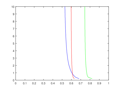
Figure 1: The blue curve is the graph of $v_{y}$ (it does not depend on $\rho$); the green and red curves are $v_{x}$ for the environments given in (4.1) with $\rho=10$ and $\rho=9$ respectively.

Figure 1 represents the ”critical” functions $v_{y}$ and $v_{x}$ for different choices of the environments. Thanks to [3], these plots give us information about how many regimes we can observe when the jump rates are modified. For example, the plot for $\rho=10$ has three regimes: extinction of $x$ (on the right of the green curve), persistence (between the green and blue curves) and extinction of $y$ (on the left of the blue curve). For $\rho=9$, there is an additional zone (above the red curve and below the blue curve) that corresponds to jump rates leading to random extinction of a species.

5 Switching between two persistent Lotka-Volterra systems

Let us assume that $\varepsilon_{0}$ and $\varepsilon_{1}$ are of Type 3. In this case, one can easily get that extinction of species $y$ is not possible if $u$ is to close of $0$ or $1$; in other words, $[0,1]\setminus\tilde{I}$ is either empty or is an open interval which closure is contained in $[0,1]$. Recall

$$R=\dfrac{\beta_{0}\alpha_{1}}{\alpha_{0}\beta_{1}},\quad A=(a_{1}-a_{0})(R-1),\quad B=(2a_{0}-c_{0}-a_{1})R+(c_{1}-a_{0}),\quad C=(c_{0}-a_{0})R.$$

Then, we get that

$$[0,1]\setminus\tilde{I}\neq\emptyset\Leftrightarrow\begin{cases}A<0\\ \Delta=B^{2}-4AC>0\\ 0<\dfrac{-B-\sqrt{\Delta}}{2A}<1.\end{cases}$$

Moreover, if $[0,1]\setminus\tilde{I}$ is nonempty, then the map $(u,v)\rightarrow\mathbb{E}[\phi(U_{u,v})]$ is (strictly) decreasing in $v$ and convex in $u$. This is a straightforward adaptation of Lemma 4.1 in [6].

Figure 2 provides the shape of $v_{x}$ and $v_{y}$ for the environments $\varepsilon_{0}=(6,1,4,2,1,5)$ and $\varepsilon_{1}=(3,3,2,5.5,5,1)$. Once again, the switched process has four regimes depending on the jump rates.

Remark 5.1.

We see a surprising result : although both vector fields are persistent, the stochastic process may lead to the extinction of one of the two species.

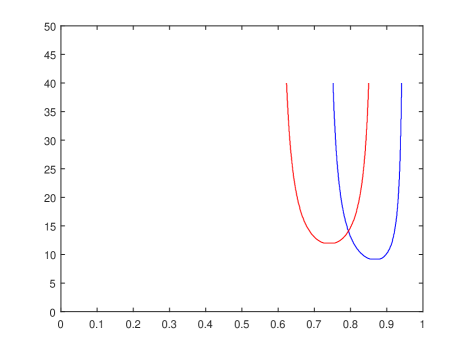
Figure 2: Graph of $v_{y}$ (blue curve) and $v_{x}$ (red curve) for the environments $\varepsilon_{0}=(6,1,4,2,1,5)$ and $\varepsilon_{1}=(3,3,2,5.5,5,1)$.

6 General case: proof of Theorem 1.4

The following array presents, for any couple of types, an example of two environments that are associated to a stochastic process with four regimes depending on the jump rates. The first line has been obtained in [3]. The second line is studied in Section 2. The fifth line is studied in Section 5. The reader can easily check that the other cases correspond to Figure 3.

$(F_{0},F_{1})$	$a_{0}$	$b_{0}$	$c_{0}$	$d_{0}$	$\alpha_{0}$	$\beta_{0}$	$a_{1}$	$b_{1}$	$c_{1}$	$d_{1}$	$\alpha_{1}$	$\beta_{1}$
Type 1-1	1	1	2	2	1	5	3	3	4	3.5	5	1
Type 1-2	1	5	2	8	3	3	2	11	1	9	2	1.8
Type 1-3	1	1	3.5	2	1	5	5	3	4	5.5	5	1
Type 1-4	1	1	2	3.5	1	5	3	4	4	3	5	1
Type 3-3	6	1	4	2	1	5	3	3	2	5.5	5	1
Type 3-4	6	1	4	8	1	5	3	10	4	7	5	1
Type 4-4	2	2	1	1	5	1	7	3.5	4	3	1	5

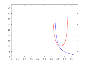
(a) Type 1-3

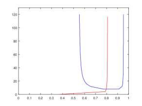
(b) Type 1-4

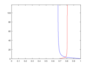
(c) Type 3-4

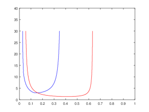
(d) Type 4-4

Figure 3: Graph of $v_{y}$ (blue curve) and $v_{x}$ (red curve) for the four last cases.

Acknowledgements.

This work has been written during the stay of Tran Hoa Phu in Tours for his intership of the French-Vietnam Master in Mathematics. We acknowledge financial support from the French ANR project ANR-12-JS01-0006-PIECE.

Florent Malrieu, e-mail: florent.malrieu(AT)univ-tours.fr

Laboratoire de Mathématiques et Physique Théorique (UMR CNRS 7350), Fédération Denis Poisson (FR CNRS 2964), Université François-Rabelais, Parc de Grandmont, 37200 Tours, France.

Tran Hoa Phu, e-mail: thphu1(AT)yahoo.com

Laboratoire de Mathématiques et Physique Théorique (UMR CNRS 7350), Fédération Denis Poisson (FR CNRS 2964), Université François-Rabelais, Parc de Grandmont, 37200 Tours, France.

References

- [1] Y. Bakhtin and T. Hurth, Invariant densities for dynamical systems with random switching, Nonlinearity 25 (2012), no. 10, 2937–2952.
- [2] M. Benaïm, S. Le Borgne, F. Malrieu, and P.-A. Zitt, On the stability of planar randomly switched systems, Ann. Appl. Probab. 24 (2014), no. 1, 292–311. MR 3161648
- [3] M. Benaïm and C. Lobry, Lotka Volterra with randomly fluctuating environments or ”how switching between beneficial environments can make survival harder”, Preprint available on arXiv number 1412.1107. To appear in Annals of Applied Probability, 2015.
- [4] M. H. A. Davis, Piecewise-deterministic Markov processes: a general class of nondiffusion stochastic models, J. Roy. Statist. Soc. Ser. B 46 (1984), no. 3, 353–388, With discussion. MR 790622
- [5] F. Malrieu, Some simple but challenging Markov processes, Ann. Fac. Sci. Toulouse Math. (6) 24 (2015), no. 4, 857–883. MR 3434260
- [6] F. Malrieu and P.-A. Zitt, On the persistence regime for Lotka-Volterra in randomly fluctuating environments, Preprint available on arXiv number 1601.08151, 2016.