Source reconstruction using a bilevel optimisation method with a smooth weighted distance function

Abstract

We consider a bilevel optimatisation method for inverse linear atmospheric dispersion problems where both linear and non-linear model parameters are to be determined. We propose that a smooth weighted Mahalanobis distance function is used and derive sufficient conditions for when the follower problem has local strict convexity. A few toy-models are presented where local strict convexity and ill-posedness of the inverse problem are explored, indeed the smooth distance function is compared and contrasted to linear and piecewise linear ones. The bilevel optimisation method is then applied to sensor data collected in wind tunnel experiments of a neutral gas release in urban environments (MODITIC).

1 Introduction

An inverse atmospheric dispersion problem is stated as follows: given the topography, the meteorological conditions and a set of detector readings determine where and when the hazardous substance was released and in which quantities. The problem is known as a source reconstruction problem, and it is easy to state but harder to solve due to being, like most inverse problems, ill-posed [1],[2]. Spurred by various applications including the locating of industrial plants [3], determining the amount of radioactive nuclides released from Chernobyl [4] and Fukushima [5], pin-pointing nuclear tests [6], estimation of material released from volcanoes [7],[8],[9] a number of different methods for addressing the inverse problem have been suggested. Even though the main difference perhaps lies in the interpretation of the results these methods are usually divided into two main categories: the probabilistic approach with its Bayesian methods and the deterministic approach with its optimisation methods. In the Bayesian setting a likelihood function is calculated and weighted with any a priori information that one has at hand to yield a posterior probability density function, which is then sampled to yield an estimate of the sought source term (see e.g. [10] for an introduction to general Bayesian inverse problems). In the deterministic setting with optimisation methods a norm is devised under which the sensor response of candidate sources is compared with the given sensor readings. The candidate source that best fits the given sensor readings (minimizes the distances under the chosen norm) is then deemed the solution to the inverse problem.

For linear inverse atmospheric dispersion problems these methods come in many different flavours and have often been devised with a given application in mind: usually there are - a priori imposed - restrictions on the source characteristics, e.g. the method may assume that the source is well localised (located at a single point in space) and that the release was instantaneous. For example Yee and coauthors have written a series of papers adapting the Bayesian method to inverse dispersion problems of increasing complexity [11],[12],[13],[14] and [15].

To use an optimisation method the inverse dispersion problem has to be cast in a manner where the distance (under a chosen norm) function between model sensor data and the given sensor readings can be minimized. Usually a least squares solution is sought, and in [16] conditions under which the least square problem is well defined is presented. Much of the literature focuses on the problem where it is a-priori assumed that there is only a single source, see e.g. [17],[18],[19] and [20]. There are however exceptions, for example in [21] the renormalisation method (least square method under the renormalisation norm) presented in [20] is generalised to cover an unknown number of point sources, and in [22] the space-time has been discretised and an optimal source term is constructed by forming a union of (space-time) grid sized point sources.

In this paper we make a contribution to the literature on optimisation methods by applying a bilevel optimisation method, see [23], to a linear inverse dispersion problem. A bilevel optimisation method splits the optimisation problem in two: into a leader (upper level) problem and a follower (lower level) problem and they are solved concurrently rather than simultaneously. We consider dispersion problems where the source is a single point source emitting at a constant rate. This problem is well suited to a bilevel optimisation method where the follower problem concerns solving for the emission rate and the leader problem pinpointing the location of the source. For the bilevel optimisation method to work properly the follower problem is required to have minima, ideally a strict minimum. We therefore study local strict convexity of the follower problem, see Theorem 1 for sufficient conditions. We then explore the concept of local strict convexity and its connection to ill-possedness of inverse problems through a few toy-model examples. Following this the paper is rounded off with the bilevel optimisation method being applied to dispersion data from a series of wind tunnel experiments of urban environments of varying complexity. The wind tunnel data was collected as part of the European Defence Agency category B project MODITIC. In all cases the boundary layer is neutrally stable, and we only consider cases where the released gas is neutrally buoyant making the dispersion problem linear.

2 Bilevel optimization problems

A bilevel optimization problem is a constrained optimization problem where the constraints also includes an optimization problem. The problem is divided into an upper level or leader problem, with decision variables $\boldsymbol{x}\in X\subseteq\mathbb{R}^{n}$, and a lower level or follower problem, with decision variables $\boldsymbol{y}\in Y\subseteq\mathbb{R}^{m}$. Here $X$ and $Y$ may be restricted to integers or nonnegative values. We follow the notation of [23], p. 6. The leader problem has the form

$$V = \min_{\boldsymbol{x}\in X}F\left(\boldsymbol{x},\boldsymbol{y}\left(\boldsymbol{x}\right)\right)$$

$$\boldsymbol{G}\left(\boldsymbol{x},\boldsymbol{y}\left(\boldsymbol{x}\right)\right) \leq \boldsymbol{0}$$

where $F$ and $\boldsymbol{G}$, respectively, are the leader objective function and constraint function, and $\boldsymbol{y}\left(\boldsymbol{x}\right)$ is an optimal solution to the follower problem

$$v\left(\boldsymbol{x}\right) = \min_{\boldsymbol{y}\in Y}f\left(\boldsymbol{x},\boldsymbol{y}\right)$$

$$\boldsymbol{g}\left(\boldsymbol{x},\boldsymbol{y}\right) \leq \boldsymbol{0}\text{.}$$

An ambiguity occurs if the follower problem has several optimal solutions, i.e., $\boldsymbol{y}\left(x\right)$ is set–valued. Then the follower is indifferent towards these points, but the leader objective may be different for different points in $\boldsymbol{y}\left(x\right)$, and there is no way for the leader to direct the follower to the upper level optimal point. Therefore, there may be no optimal solution to the bilevel program although all functions are continuous and $X,Y$ are compact, cf. [23], p. 11. In our problem the sets $X,Y$ will be positive orthants, the follower objective function $f\left(\boldsymbol{x},\boldsymbol{y}\right)$ will be a Mahalanobis distance function measuring the discrepancy between model data and measurements. The leader objective function $F$ will have the form

$$F\left(\boldsymbol{x},\boldsymbol{y}\right)=\exp\left(-\lambda\sum y_{i}\right)+f\left(\boldsymbol{x},\boldsymbol{y}\right)$$

hence minimizing the least square function, but penalizing large values of $\boldsymbol{y}$, which will act as a regularization of the problem ($\lambda>0$ is a regularization parameter).

3 The follower problem

In the setting we are considering we have a priori assumed that the source is a point source releasing a neutrally buoyant substance at a constant rate. Under these assumptions the source location $\boldsymbol{x}\in\mathbb{R}^{d}$ is a nonlinear model parameter while the emission rate $\boldsymbol{y}\in\mathbb{R}^{1}$ is a linear model parameter. In general, our model formulation allows a linear combination of basic sources, with a linear positive weight vector $y\in\mathbb{R}^{n}$. To solve the inverse problem we need a source-sensor relationship. Since the problem is linear the source-sensor relationship is given a matrix relationship, which for computational efficiency [3] is expressed through the adjoint formulation of the problem, thus $A:\mathbb{R}^{d}\rightarrow\mathbb{R}_{+}^{m\times n}$ is a matrix function with nonnegative elements (no sinks are considered) and the adjoint model data $\boldsymbol{\mu}=\boldsymbol{\mu}\left(\boldsymbol{x},\boldsymbol{y}\right)=A\left(\boldsymbol{x}\right)\boldsymbol{y}\in\mathbb{R}^{m}$. The measured data $\boldsymbol{z}\in\mathbb{R}^{m}$ is the sensor response.
We regard $\boldsymbol{z}$ as a random vector, and we assume that the adjoint model data $\boldsymbol{\mu}$ represent the mean of $\boldsymbol{z}$. We also assume that the components $z_{i}$ of $\boldsymbol{z}$ are statistically independent and that the variance of $z_{i}$ is

$$var\left(z_{i}\right)=\sigma^{2}\left(\mu_{i}\right)$$

where $\sigma:\mathbb{R\rightarrow R}_{+}$ is a given function. We let the follower objective function be the Mahalanobis distance between $\boldsymbol{z}$ and $\boldsymbol{\mu}$, viz.,

$$f\left(\boldsymbol{x},\boldsymbol{y}\right)=\sum_{i=1}^{m}\frac{\left(z_{i}-\mu_{i}\right)^{2}}{\sigma^{2}\left(\mu_{i}\right)}\text{.}$$ (1)

In particular, we want to be able to choose a scale invariant distance function, giving equal emphasis to all $\mu_{i}$, regardless of their size.

3.1 Local convexity of the follower problem

If the follower problem is strictly convex, the follower problem has a unique optimal solution $\boldsymbol{y}\left(\boldsymbol{x}\right)$ for each $\boldsymbol{x}\in X$, and by mild assumptions on $f\left(\boldsymbol{x},\boldsymbol{y}\right)$, an envelope theorem holds (e.g., [24], Theorem 2, p. 586), which implies that the optimal value function

$$V\left(\boldsymbol{x}\right)=f\left(\boldsymbol{x},\boldsymbol{y}\left(\boldsymbol{x}\right)\right)=\inf_{\boldsymbol{y\in Y}}\;f\left(\boldsymbol{x},\boldsymbol{y}\right)$$

is continuous. Therefore, the leader problem

$$\inf_{\boldsymbol{x\in X}}F\left(\boldsymbol{x},\boldsymbol{y}\left(\boldsymbol{x}\right)\right)$$

has a solution since

$$F\left(\boldsymbol{x},\boldsymbol{y}\left(\boldsymbol{x}\right)\right)=\exp\left(-\lambda\sum_{i}y_{i}\left(\boldsymbol{x}\right)\right)V\left(\boldsymbol{x}\right)\text{. }$$

However, in our setting the only situation when the follower problem is guaranteed to be strictly convex is when $\sigma\left(\mu\right)$ is constant, i.e., the classical least square method. However, we may derive conditions for local convexity, as the following theorem shows.

Theorem 1

Assume that

$$f\left(y_{1},...,y_{n}\right)=\sum_{i=1}^{m}\frac{r_{i}^{2}}{\sigma^{2}\left(\mu_{i}\right)}$$ (2)

where

$$\mu_{i} = \sum_{j}a_{ij}y_{j}$$

$$r_{i} = z_{i}-\mu_{i}\text{. }$$

and $A=\left(a_{ij}\right)\in\mathbb{R}^{m\times n}$. Consider a fixed $\boldsymbol{y}$ and suppose that $\sigma$ is positive and twice continuously differentiable in a neigbourhood of $\mu$.Then

$$\frac{\partial f}{\partial y_{k}} = -2\sum_{i}a_{ik}\rho\left(\mu_{i},r_{i}\right)\frac{r_{i}^{2}}{\sigma^{2}\left(\mu_{i}\right)}$$

$$\frac{\partial^{2}f}{\partial y_{k}\partial y_{l}} = 2\sum_{i}a_{ik}a_{il}\eta\left(\mu_{i},r_{i}\right)\frac{r_{i}^{2}}{\sigma^{2}\left(\mu_{i}\right)}$$

where

$$\rho\left(\mu,r\right) = \frac{1}{r}+\frac{\sigma^{\prime}\left(\mu\right)}{\sigma\left(\mu\right)}$$

$$\eta\left(\mu,r\right) = \left(\frac{1}{r}+2\frac{\sigma^{\prime}\left(\mu\right)}{\sigma\left(\mu\right)}\right)^{2}-\left(\left(\frac{\sigma^{\prime}\left(\mu\right)}{\sigma\left(\mu\right)}\right)^{2}+\frac{\sigma^{\prime\prime}\left(\mu\right)}{\sigma\left(\mu\right)}\right)\text{.}$$

Moreover, if $A$ has full rank then

1. If $\eta\left(\mu_{i},r_{i}\right)>0$ for all $i$ then $f$ is strictly convex in a neighborhood of $\boldsymbol{y}$.

2. If $\eta\left(\mu_{i},r_{i}\right)<0$ for all $i$ then $f$ is strictly concave in a neigborhood of $\boldsymbol{y}$.

Proof. The formulas for the first and second derivatives of $f$ are proved by elementary but tedious calculations, using the chain rule and the quotient rule for differentiation. If $A$ has full rank, and $\eta\left(\mu_{i},r_{i}\right)>0$ for all $i$, then

$$H\left(\boldsymbol{u}\right)\equiv\sum_{k,l}u_{k}\frac{\partial^{2}f}{\partial y_{k}\partial y_{l}}u_{l}=\sum_{i}\sum_{k,l}\psi_{i}a_{ik}u_{k}\psi_{i}a_{il}u_{l}=\sum_{i}\left(\sum_{k}\psi_{i}a_{ik}u_{k}\right)^{2}$$

for all $\boldsymbol{u}\in\mathbb{R}^{n}$,where

$$\psi_{i}=\sqrt{\eta\left(\mu_{i},r_{i}\right)\frac{r_{i}^{2}}{\sigma^{2}\left(\mu_{i}\right)}}\text{.}$$

Hence $H\left(\boldsymbol{u}\right)\geq 0$. Assume that $H\left(\boldsymbol{u}\right)=0$. Then $\sum_{k}\psi_{i}a_{ik}u_{k}=0$ for all $i$. Note that $\psi_{i}>0$, since when $r\rightarrow 0$ we have

$$\eta\left(\mu,r\right)\frac{r^{2}}{\sigma^{2}\left(\mu\right)}\rightarrow\frac{1}{\sigma^{2}\left(\mu\right)}>0\text{. }$$

Hence $\boldsymbol{u}=0$, since the vectors $\boldsymbol{v}_{i}=\left(\psi_{i}a_{i1},\psi_{i}a_{i2},...,\psi_{i}a_{in}\right)$, $i=1,2,...,m$ span $\mathbb{R}^{n}$. This shows that $H$ is positive definite at $\boldsymbol{y}$. By continuity, $H$ is positive definite, and hence $f$ strictly convex, in a neighborhood of $\boldsymbol{y}$. Similarly, if $A$ has full rank and $\eta\left(\mu_{i},r_{i}\right)<0$, then

$$H\left(\boldsymbol{u}\right)\equiv\sum_{k,l}u_{k}\frac{\partial^{2}f}{\partial y_{k}\partial y_{l}}u_{l}=-\sum_{i}\left(\sum_{k}\psi_{i}a_{ik}u_{k}\right)^{2}$$

where

$$\psi_{i}=\sqrt{-\eta\left(\mu_{i},r_{i}\right)\frac{r_{i}^{2}}{\sigma^{2}\left(\mu_{i}\right)}}$$

and it follows with a similar argument as above that $f$ is strictly concave in a neighborhood of $\boldsymbol{y}$.   

Most inverse modelling methods works perfectly for synthetic data, i.e. when the ”observed” sensor response is calculated using a dispersion model (the same dispersion model that is then used to solve the inverse problem). Indeed showing that an inverse modelling method works well for synthetic data and, in particular, slightly perturbed synthetic data is usually included in the body of work motivating the method. In view of the theorem we make the following observation.

Remark 2

Note that when $r\rightarrow 0$, then $\eta\left(\mu,r\right)\rightarrow\infty$, so for small enough $r$, $\eta$ is always positive, if $\mu$ is restricted to a compact set. Hence for $\boldsymbol{z}$ sufficiently close to $\mathbf{\mu}\left(\boldsymbol{y}\right)$, $f\left(\boldsymbol{y}\right)$ is convex. This explains why most methods work well on synthetic model data with small perturbations.

We will now restrict ourselves to functions $\sigma\left(\mu\right)$ which are continuous, increasing, convex, and positive for $\mu>0$, and satisfying

$$\lim_{\mu\rightarrow\infty}\frac{\sigma\left(\mu\right)}{\mu}=1\text{. }$$

Moreover, we assume that $\sigma$ is twice continuously differentiable, except possibly at a finite number of points. Hence $\sigma^{\prime\prime}\left(\mu\right)\geq 0$ at all points where $\sigma^{\prime\prime}$ exists. Note that if $\sigma\left(\mu\right)$ satisfies these conditions, so does

$$\sigma_{\delta}\left(\mu\right)\equiv\delta\sigma\left(\mu/\delta\right)$$

for any $\delta>0$, so the class of functions $\sigma$ we consider is scale–invariant. We consider three examples:

$$\sigma\left(\mu\right) = erf\left(\mu\right)-2\left(1-\frac{1}{\sqrt{\pi}}\right)\exp\left(-\mu^{2}\right)\text{ (Smooth threshold)}$$

$$\sigma\left(\mu\right) = \max\left(1,\mu\right)\text{ (Piecewise linear)}$$ (3)

$$\sigma\left(\mu\right) = \mu\text{ (Linear)}$$

Figure 1: Graphs of the three considered $\sigma$–functions.

Recall that

$$f\left(\boldsymbol{y}\right)=\sum_{i}\frac{\left(z_{i}-\mu_{i}\right)^{2}}{\sigma^{2}\left(\mu_{i}\right)}$$

Since we assume that $\sigma^{\prime\prime}\geq 0$ and $\sigma>0$ for $\mu>0$, we can write $\eta$ on the form

$$\eta=\left(\frac{1}{r}-\alpha\right)\left(\frac{1}{r}-\beta\right)$$

where

$$\alpha\left(\mu\right) = -2\frac{\sigma^{\prime}\left(\mu\right)}{\sigma\left(\mu\right)}-\sqrt{\left(\frac{\sigma^{\prime}\left(\mu\right)}{\sigma\left(\mu\right)}\right)^{2}+\frac{\sigma^{\prime\prime}\left(\mu\right)}{\sigma\left(\mu\right)}}$$

$$\beta\left(\mu\right) = -2\frac{\sigma^{\prime}\left(\mu\right)}{\sigma\left(\mu\right)}+\sqrt{\left(\frac{\sigma^{\prime}\left(\mu\right)}{\sigma\left(\mu\right)}\right)^{2}+\frac{\sigma^{\prime\prime}\left(\mu\right)}{\sigma\left(\mu\right)}}$$

Clearly, $\eta>0$ if and only if the two factors have the same sign, i.e., $1/r\in\left[\alpha,\beta\right]^{c}$, and $\eta<0$ if and only if $1/r\in\left(\alpha,\beta\right)$. To analyze these conditions further we need to consider the cases when $\alpha,\beta$ have the same sign and when they have different signs. If $\alpha,\beta$ have the same sign then $1/r\in\left(\alpha,\beta\right)$ if and only if $r\in\left(1/\beta,1/\alpha\right)$ (this includes the limiting cases $\beta\nearrow 0$ or $\alpha\searrow 0$, with $1/\beta=-\infty$ and $1/\alpha=\infty$). If $\alpha,\beta$ have different signs, i.e., $\alpha<0<\beta$, then $1/r\in\left(\alpha,\beta\right)$ if and only if $r\in\left[1/\alpha,1/\beta\right]^{c}$. By the assumptions on $\sigma$, $\alpha$ and $\beta$ are defined everywhere except possibly at a finite number of points. Henceforth, we only consider points where $\alpha$ and $\beta$ are defined. We can now conclude that $\eta<0$ if and only if either i) $z-\mu\in\left(\beta^{-1},\alpha^{-1}\right)$ and $\alpha<\beta\leq 0$, or ii) $z-\mu\in\left[\alpha^{-1},\beta^{-1}\right]^{c}$ and $\alpha<0<\beta$, or iii) $z-\mu\in\left(\beta^{-1},\infty\right)$ and $0=\alpha<\beta$. Likewise, we can conclude by complementarity that $\eta>0$ if and only if either i) $z-\mu\in\left[\beta^{-1},\alpha^{-1}\right]^{c}$ and $\alpha<\beta\leq 0$, or ii) $z-\mu\in\left(\alpha^{-1},\beta^{-1}\right)$ and $\alpha<0<\beta$, or iii) $z-\mu\in\left(-\infty,\beta^{-1}\right)$ and $0=\alpha<\beta$ or iv) $\alpha=\beta=0$.

Relying on these inequalities we can find domains where a distance function is guaranteed to be strictly convex or strictly concave.

Example 3

Consider $\sigma\left(\mu\right)=\mu$, the linear case. Then $\alpha(\mu)=-3/\mu$ and $\beta(\mu)=-1/\mu$. Hence $\alpha^{2}>\beta$ and $\eta\left(\mu,r\right)>0$ if and only if $r\in\left(-\infty,-\mu\right)\cup\left(-\mu/3,\infty\right)$, i.e., $z=\mu+r\in\left(-\infty,0\right)\cup\left(2\mu/3,\infty\right)$. Moreover, $\eta\left(\mu,r\right)<0$ if and only if $z=\mu+r\in\left(0,2\mu/3\right)$. Hence for fixed $\boldsymbol{z}$, $f$ is strictly convex on the set $\cap_{i}\left\{2\mu_{i}\left(\boldsymbol{y}\right)/3<z_{i}\right\}$, and strictly concave on the set $\cap_{i}\left\{2\mu_{i}\left(\boldsymbol{y}\right)/3>z_{i}\right\}$. Let for example

$$A=\begin{bmatrix}1&0\\ 0&1\\ 1&1\end{bmatrix}\text{, }z=\begin{bmatrix}1\\ 1\\ 5/3\end{bmatrix}\text{.}$$

Then

$$f\left(y_{1},y_{2},y_{3}\right)=\frac{\left(1-y_{1}\right)^{2}}{y_{1}^{2}}+\frac{\left(1-y_{2}\right)^{2}}{y_{2}^{2}}+\frac{\left(3-y_{1}-y_{2}\right)^{2}}{\left(y_{1}+y_{2}\right)^{2}}\text{,}$$

and $f$ is strictly convex on $\left\{\left(y_{1},y_{2},y_{3}\right)\in\mathbb{R}_{+}^{3}\mid 2y_{1}/3<1\text{, }2y_{2}/3<1\text{,}2\left(y_{1}+y_{2}\right)/3<5/3\right\}$, and strictly concave on $\left\{\left(y_{1},y_{2},y_{3}\right)\in\mathbb{R}_{+}^{3}\mid 2y_{1}/3>1\text{, }2y_{2}/3>1\text{,}2\left(y_{1}+y_{2}\right)/3>5/3\right\}$ (the last condition is not active). Of course, $f$ may be strictly convex or concave on points outside these sets also; these conditions are sufficient, but not necessary. The domains of local convexity and local concavity are plotted in the next figure.

Figure 2: This figure shows isocurves of $f\left(y_{1},y_{2}\right)$, the local convexity region (blue) and the local concavity region (red), determined from Theorem 1. The minimum point is marked with a red circle.

Remark 4

When $\sigma$ is rescaled (i.e., replacing $\sigma\left(\mu\right)$ by $\sigma_{\delta}\left(\mu\right)$), the derivatives are scaled according to $\sigma_{\delta}^{\prime}\left(\mu\right)=\sigma^{\prime}\left(\mu/\delta\right)$ and $\sigma_{\delta}^{\prime\prime}=\delta^{-1}\sigma^{\prime\prime}\left(\mu/\delta\right)$, and hence $\alpha\left(\mu\right)$ is replaced by $\alpha_{\delta}\left(\mu\right)=\delta^{-1}\alpha\left(\mu/\delta\right)$, and $\beta\left(\mu\right)$ is replaced by $\beta_{\delta}\left(\mu\right)=\delta^{-1}\beta\left(\mu/\delta\right)$.

3.2 Examples of follower problems with unique and non-unique solutions

In Theorem 1 we established sufficient conditions for the objective function $f$ to be locally strictly convex with the view of determining when the follower problem is well posed. Alas, strict convexity of the objective function is not sufficient to make the follower problem convex as the constraints have to be taken into account. We explore the interplay between the objective function and the constraints and their effect on minima and well posedness of the minimization problem through a series of examples. It is instructive to begin with the linear case $\sigma(\mu)=\mu$, and then proceed to the nonlinear cases (smooth threshold and piecewise linear), compare (3).

3.2.1 The linear case

In the linear case, the minimization problem for $f$ can be formulated as a constrained minimization problem with a convex objective function. However, the constraints are not convex, which can cause multiple minimum points for certain values of $A$ and $\boldsymbol{z}$. For $\sigma\left(\mu\right)=\mu$, $f$ is a strictly convex function of $\boldsymbol{\xi}\equiv\boldsymbol{\mu}^{-1}=\left(\mu_{1}^{-1},...,\mu_{m}^{-1}\right)$:

$$f\left(\boldsymbol{y}\right)=F\left(\boldsymbol{\xi}\right)\equiv\sum_{i}\left(z_{i}\xi_{i}-1\right)^{2}\text{.}$$

Writing $F$ on the form

$$F\left(\boldsymbol{\xi}\right)=\sum_{i:b_{i}\neq 0}\frac{\left(\xi_{i}-z_{i}^{-1}\right)^{2}}{\left(z_{i}^{-1}\right)^{2}}+m-m^{\prime}\text{,}$$

where $m^{\prime}=\sum_{i:b_{i}\neq 0}1$ is the number of $b_{i}\neq 0$, we see that for $c>0$, the level surface $F\left(\boldsymbol{\xi}\right)=c+m-m^{\prime}$ is an $m^{\prime}$–axial ellipsoidal cylinder with center coordinates $\xi_{i}=z_{i}^{-1}$ and corresponding semiaxes $\sqrt{c}z_{i}^{-1}$ for all $i$ such that $z_{i}\neq 0$, extending linearly along all coordinates $\xi_{i}$ for which $z_{i}=0$. Let us assume that all $z_{i}\neq 0$ for simplicity. Then for $c>0$ the level surface $F\left(\boldsymbol{\xi}\right)=c$ is an $m$–axial ellipsoid centered at $\left(z_{1}^{-1},...,z_{m}^{-1}\right)$ with semiaxes $\sqrt{c}z_{1}^{-1},...,\sqrt{c}z_{m}^{-1}$. The minimization problem for $f$ can be formulated as a constrained minimization problem

$$\min F\left(\boldsymbol{\xi}\right)$$

$$\boldsymbol{G}\left(\boldsymbol{\xi},\boldsymbol{y}\right) \leq \boldsymbol{0}$$

$$\boldsymbol{H}\left(\boldsymbol{\xi},\boldsymbol{y}\right) = \boldsymbol{0}$$

where $\boldsymbol{G}\left(\boldsymbol{\xi},\boldsymbol{y}\right)=-\boldsymbol{y}$, and $\boldsymbol{H}=\left(H_{1},...,H_{m}\right)$, where

$$H_{i}\left(\boldsymbol{\xi},\boldsymbol{y}\right)=\varphi_{i}\left(\boldsymbol{y}\right)-\xi_{i}\text{, }i=1,...,m$$

and

$$\varphi_{i}\left(\boldsymbol{y}\right)=\frac{1}{\left(A\boldsymbol{y}\right)_{i}}\text{.}$$

The objective function $F\left(\boldsymbol{\xi},\boldsymbol{y}\right)=F\left(\boldsymbol{\xi}\right)$, is convex, and depends on $\boldsymbol{z}$, but is independent of $A$. The inequality constraints are linear and hence convex. The equality constraints depend on $A$, but are independent of $\boldsymbol{z}$, and are not convex, so the problem is not convex. We have thus separated the dependencies of $A$ and $\boldsymbol{z}$ into the objective and constraint functions, respectively.

The equality constraints $\boldsymbol{H}\left(\boldsymbol{\xi},\boldsymbol{y}\right)=\boldsymbol{0}$ define an $n$–dimensional parametrized surface $S$ in $\mathbb{R}^{m}$ by $\boldsymbol{\xi}=\boldsymbol{\varphi}\left(\boldsymbol{y}\right)$. The $n$–dimensional tangent space to $S$ at $\boldsymbol{\varphi}\left(\boldsymbol{y}\right)$ is spanned by the tangent vectors

$$\frac{\partial\boldsymbol{H}}{\partial y_{j}}\left(\boldsymbol{y}\right)\text{, }j=1,...,n\text{. }$$

The Karush-Kuhn-Tucker (KKT) conditions (see e.g. [25]) for the minimization problem are

$$-\frac{\partial F}{\partial\xi_{i}} = \sum_{k=1}^{n}\mu_{k}\frac{\partial G_{k}}{\partial\xi_{i}}+\sum_{l=1}^{m}\lambda_{l}\frac{\partial H_{l}}{\partial\xi_{i}}=\lambda_{i}\text{, }i=1,...,m$$

$$0 = -\frac{\partial F}{\partial y_{j}}=\sum_{k=1}^{n}\mu_{k}\frac{\partial G_{k}}{\partial y_{j}}+\sum_{l=1}^{n}\lambda_{l}\frac{\partial H_{l}}{\partial y_{j}}\text{, }j=1,...,n$$

$$\mu_{j}G_{j} = 0\text{, }j=1,...,n$$

$$\mu_{j} \geq 0\text{, }j=1,...,n$$

which are necessary conditions for minimum. Assume for simplicity that we have a minimum with $\boldsymbol{y}^{\ast}>0$. Then $G_{j}<0$ so $\mu_{j}=0$. Substituting the first equation in the second we get

$$\sum_{l=1}^{m}\frac{\partial F}{\partial\xi_{l}}\frac{\partial H_{l}}{\partial y_{j}}=0\text{, }j=1,...,n\text{.}$$

Geometrically, this conditions means that the gradient of $F$ is orthogonal to the tangent space of $S$ at $y^{\ast}$. Hence, in the $\boldsymbol{\xi}$–space, minimal points $\boldsymbol{y}^{\ast}$ are characterized by points $\boldsymbol{\xi}^{\ast}=\boldsymbol{\varphi}\left(\boldsymbol{y}^{\ast}\right)$ where the $n$–dimensional surface $S:\boldsymbol{\xi}=\boldsymbol{\varphi}\left(\boldsymbol{y}\right)$ is tangent to the ellipsoid $F\left(\boldsymbol{\xi}\right)=c^{\ast}$. The optimal value is then $c^{\ast}$.

Suppose now that $A$ is fixed. For $\boldsymbol{z}$, the center of the ellipsoidal isosurfaces of $F$, let $E\left(\boldsymbol{z}\right)$ denote the smallest isosurface of $F$ that intersects $S$. For generic $\boldsymbol{z}$, the ellipsoid $E\left(\boldsymbol{z}\right)$ will contain only one point $\boldsymbol{\varphi}\left(\boldsymbol{y}^{\ast}\right)$, defined by the unique minimum point $\boldsymbol{y}^{\ast}$. However, for $\boldsymbol{z}$ in some exceptional lower–dimensional set, $E\left(\boldsymbol{z}\right)$ will touch $S$ at several points, in which case we have several minimum points $\boldsymbol{y}^{\ast}$. In that case, $A$ or $\boldsymbol{z}$ can be perturbed so that either of the multiple minima is perturbed into a single global minimum. Hence the global minimum point varies discontinuously with $A$ and $\boldsymbol{z}$, and the problem is ill posed (unless $\boldsymbol{z}$ is restricted to be generic, e.g., if $\boldsymbol{z}^{-1}$ is sufficiently close to the surface $S$).

Example 5

Let

$$A=\begin{bmatrix}1&\varepsilon\\ \varepsilon&1\\ 1&1\end{bmatrix}\text{, }\boldsymbol{z}=\begin{bmatrix}1\\ 1\\ t\end{bmatrix}$$

where $\varepsilon=0.1$.

Figure 3: Case $t=3$. The figure shows minimum point $\xi^{\ast}=\left(0.7729,0.7729,0.4251\right)$ as a red dot, the surface $S$ parametrized for $0.5\leq y_{1},y_{2}\leq 5$, and the ellipsoidal isosurface for $f$ with optimal value $c^{\ast}=0.17893$. The center $\boldsymbol{z}$ of the ellipsoid is marked by a blue cross.

Figure 4: Case $t=3$. The figure shows the minimum point $y^{\ast}=\left(1.1762;1.1762\right)$ marked with a red circle, with the minimal value $c^{\ast}=0.17893$. Also isocurves for $f$ are shown.

Figure 5: Case $t=5.$, two minimum points $\xi_{1}^{\ast}=\left(0.9303,0.2920,0.2444\right)$, $\xi_{2}^{\ast}=\left(0.2920,0.9303,0.2444\right)$ marked by red dots, parametric surface $S$ plotted for $0.5\leq y_{1},y_{2}\leq 5$, and ellipsoidal isosurface for $f$  and optimal value $c^{\ast}=0.55556$. The center $\boldsymbol{z}$ of the ellipsoid is marked by a blue cross.

Figure 6: Case $t=5$. Two minimal points $y_{1}^{\ast}=\left(0.73987,3.351\right)$, $y_{2}^{\ast}=\left(3.351,0.73987\right)$, marked by red circles. Minimum value $c^{\ast}=0.55556$. Isosurfaces for $f$ also shown.

The one–dimensional case

Distinct minima cannot occur in the case $n=1$. We have

Proposition 6

If $a_{i}>0$, and some $b_{i}>0$ then

$$f\left(y\right)=\sum_{i=1}^{m}\frac{\left(b_{i}-a_{i}y\right)^{2}}{\left(a_{i}y\right)^{2}}=m-\frac{\alpha^{2}}{\beta}+\beta\left(y^{-1}-\frac{\alpha}{\beta}\right)^{2}$$

where

$$\chi_{i}=b_{i}/a_{i}\text{, }\alpha=\sum_{i}\chi_{i}\text{ and }\beta=\sum_{i}\chi_{i}^{2}\text{, }$$

and $f$ has minimum value $m-\alpha^{2}/\beta$, attained for

$$y=\frac{\beta}{\alpha}\text{,}$$

which is a strict minimum. Moreover, the minimum point $y$ depends continuously on $a_{i}$, $b_{i}$, so the minimization problem is well–posed.

Proof. The formula for $f$ is proved by elementary calculations. The final conclusion follows from the observation that $f\left(y\right)$ is a second order polynomial in $y^{-1}$.   

Remark 7

Note that $\partial\chi_{i}/\partial a_{i}=-a_{i}^{-1}\chi_{i}^{2}$ and $\partial\chi_{i}/\partial b_{i}=a_{i}^{-1}$, and the sensitivity of the minimum point $y=y\left(a_{1},...,a_{m},b_{1},...,b_{m}\right)$ is given by

$$\frac{\partial y}{\partial a_{i}}=\frac{1}{a_{i}}\frac{\left(y-2\chi_{i}\right)\chi_{i}^{2}}{\alpha}\text{, }\frac{\partial y}{\partial b_{i}}=\frac{1}{a_{i}}\frac{2\chi_{i}-y}{\alpha}$$

so the minimum point $y$ is very sensitive for $a_{i}$ and $b_{i}$ when $a_{i}$ is small, provided that $y\neq 2\chi_{i}$.

3.2.2 The nonlinear case

In contrast to the linear case, $f$ can have multiple local minima for $n=1$ in the nonlinear case. For certain values of $A$,$\boldsymbol{z}$, these minimum values may be identical, hence distinct global minima. When this occurs, the minimum problem becomes ill–posed, as the following example shows.

Example 8

Let

$$A=\begin{bmatrix}0.3\\ 0.8\end{bmatrix}\text{, }\boldsymbol{z}=\begin{bmatrix}t\\ 0\end{bmatrix}\text{, }\delta=1$$

and

$$f\left(y\right)=\sum_{i=1}^{m}\frac{\left(z_{i}-a_{i}y\right)^{2}}{\sigma^{2}\left(a_{i}y\right)}\text{, }i=1,2\text{. }$$

If $t=t_{0}\approx 1.0732$, then $f$ has two distinct global minimum points for the smooth threshold $\sigma(\mu)$, (the smooth threshold is defined in equation (3)), see Figure 7. Moreover, for all $t$ in a neighborhood $U$ of $t_{0}$, $f$ has two distinct local minima . For $t<t_{0}$ in $U$, the left local minimum of $f$ is global, and for $t>t_{0}$ in $U$, the right local minimum of $f$ is global. Hence when $t$ increases from $t=1.05$ to $1.10$, the global minimum point $y=y\left(t\right)$ of $f\left(y\right)$ jumps from $y\approx 0.4919$ to $y\approx 3.5733$ at $t=t_{0}$, see figures 8 and 9. The function $f$ shows a similar behaviour for the piecewise linear $\sigma$, with a slightly different value of $t_{0}$.

Figure 7: The figure shows $f\left(y\right)$ for $t=t_{0}\approx 1.0732$. At this transition point, the smooth threshold $\sigma$ gives two distinct global minima, while the piecewise linear $\sigma$ gives a single global minimum to the right. The transition point for the piecewise linear $\sigma$ occurs for a sligthly different value of $t$.

Figure 8: The figure shows $f\left(y\right)$ for $t=1.05$. Both smooth threshold and piecewise linear $\sigma$ give two distinct local minima, the left one is also global minimum.

Figure 9: The figure shows $f\left(y\right)$ for $t=1.10$. Both smooth threshold and piecewise linear $\sigma$ give two distinct local minima, the right one is also global minimum.

In higher dimensions, nonlinear $\sigma$ give similar behaviour of $f$ regarding multiple global minima and ill–posedness of the minimization problem.

In higher dimensions, the nonlinear $\sigma$ functions causes a similar behaviour as the linear $\sigma$ regarding multiple local minimas of $f$. To illustrate this, we show a slight perturbation of the bimodal example, Example 5, above for the linear $\sigma$. The perturbed problem still have two local minima, but only one of them is a global min. Let

$$A=\begin{bmatrix}1&0.1\\ 0.1&1\\ 1&1\end{bmatrix}\text{, }\boldsymbol{z}=\begin{bmatrix}1.1\\ 0.9\\ 5\end{bmatrix}\text{.}$$

Then we get

Figure 10: Both smooth threshold and piecewise linear $\sigma$ functions give two local minima in this case, and quite similar isocurve pattern. Comparison with the linear case, Figure 6, in the previous example reveals a similar pattern.

In some cases there are huge differences between smooth threshold and piecewise linear $\sigma$. For example, by randomly choosing $A$ and $\boldsymbol{z}$, we found

$$A=\begin{bmatrix}0.0557&0.8528\\ 0.3231&0.6868\\ 0.9336&0.1672\end{bmatrix}\text{, }\boldsymbol{z}=\begin{bmatrix}1.3196\\ 0\\ 1.3499\end{bmatrix}$$

which gives

Figure 11: Here we see a dramatic difference between the discontinouous gradient and double local minima in the piecewise linear case, and the smooth, single global minimum in the smooth threshold and linear cases.

A motivation for using a scaled piecewise linear $\sigma$ rather than the linear $\sigma$ is that model values $\mu$ (averages) below a detection limit should give a variance $\sigma$ of the measurement value $z$ which is independent of $\mu$ (corresponding to the background noise). We think it is a good compromise to use the smooth threshold $\sigma$, giving a variance with a strictly positive lower bound, but avoiding potential numerical difficulties as pictured in Figure 11 above.

4 Application: neutral gas in an urban environment

We will now apply the bilevel optimisation method to experimental data reconstructing the source term. The different choices of distance function, smooth threshold, piecewise linear, linear and constant will be compared and contrasted. The experimental data stems from the European Defence Agency category B project MODITIC where wind tunnel experiments were conducted involving release of both neutrally buoyant gas as well as dense gas over urban environments of varying complexity. In all cases the wind tunnel boundary layer was neutrally stable. The gas was released from a single point source either as a puff or continuously at a constant rate. For the full details on the experimental set up we refer to [26] and [27].

4.1 Sensor data

As the bilevel optimisation method described above is designed for linear inverse dispersion problems we only consider cases where the released gas is neutrally buoyant, and to further reduce the scope we focus on two scenarios referred to as the simple array, a symmetric case with four buildings, and the complex array, a less symmetric case involving fourteen buildings.

4.1.1 The simple array

The dimensions of the simple array, with the positions of the synchronized detectors we use for backtracking is shown in Figure 12.

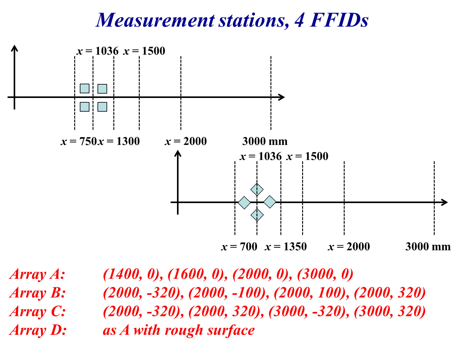
Figure 12: Sensors network (A, B, C arrangement) for the simple array cases. In each scenario 4 synchronized detectors are used to measure the concentration of the released gas. The dectors are located at the positions stated under A, B and C respectively.

The wind direction in the wind tunnel experiments is aligned with the x-axis in Figure 12, and as shown in the figure the simple array may aligned at two different angles: we denote the alignment in the upper pane as “0 degrees” and the alignment in the lower pane as “45 degrees”. In each scenario four synchronized detectors were used, hence the reference 4 FFID in Figure 12, and we chose three different sets of locations for these detectors: we refer to these as case A, B and C. In addition to this two different source locations were available: these we denote S1 and S2, both S1 and S2 (at the origin) are located at 8H upwind (=-0.88m) in the x direction, but S1 is shifted off the x-axis by 1.5H (=0.165m) in the +y direction. The location of S2 was chosen to be the origin of the coordinate system. The diameter of the sources is 0.1m (to be compared to building height and sides of H=0.11m). A constant release rate of 50l/min=8.33e-4 m³/s was used in all scenarios.

4.1.2 The complex array

In the complex array there more buildings present and there is less symmetry. The configuration also opens up for a larger number of sensible detector locations, however, still only 4 synchronized detectors were used in these scenarios. For the complex array we chose five different sets of detector configurations: these are denoted case A through to E, and these are shown together with the geometry of the complex array in Figure 13. Note that some detectors are located on the roof tops (cases A and C) and other are inside the street canyons (cases B, D and E).

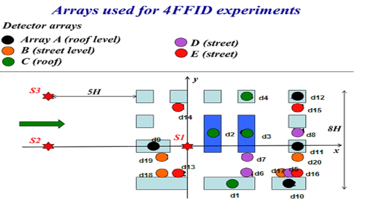
Figure 13: Configuration of the complex array. In each scenario, denoted case A through to E, 4 synchronized detectors were used to measure the concentration of the released gas. Note that some detectors are located at the roof of the buildings. Two different source locations were used, denoted S1 and S2. (There is a third source S3 indicated in the figure, but it was not used for inverse modelling).

Two different source locations were used S1 and S2. The diameter of the sources is 0.1m. The source S1 is defined to be at the origin (see Figure 13) while S2 is located upwind at x=-8H=-0.88m and y=0. S1 and S2 are both located on the ground. As for the empty and complex array the source strength is 50l/min=8.33e-4m³/s.

4.2 Source-sensor relationship: adjoint CFD-plumes

To apply the bilevel optimisation method to the sensor data retrieved from the wind tunnel we need a relationship between the source and the sensors, i.e. a dispersion model. Since we are in a setting where a) we are considering an urban environment and b) we are trying to gauge the fidelity of the inverse solver, we opt to use a computational fluid dynamics solver for the wind field. We are only considering the steady state of the dispersion scenario (not the transient behaviour when the source is turned on and subsequently off), hence a Reynolds-averaged Navier-Stokes (RANS) solver is suitable. See [28] for RANS solutions of MODITIC scenarios. The RANS solution in each case defines a source-sensor relationship which could be used to solve the inverse problem, however, due to computational efficiency it is preferable to solve the adjoint dispersion problem [3]. The dispersion problem is self-adjoint, hence the adjoint solution is obtained by reversing the advection while leaving the diffusive component untouched. The RANS solver in PHEONICS was adapted accordingly to yield adjoint RANS solutions for the simple array and the complex array [29]. One adjoint wind field was computed for each sensor. These adjoint flow fields constitute a source-sensor relationship.

4.3 Source reconstruction

We will briefly outline the bilevel optimisation algorithm before using it to reconstruct the MODITIC sources.

4.3.1 Bilevel optimisation algorithm

In each case four synchronous sensors where used, let us number them $i=1,2,3,4$. For each sensor $i$ compute the adjoint dispersion plume $\chi_{i}(x,y,z)$ for each grid point $(x,y,z)$. Using the adjoint plume the model sensor data is given by $c_{i}=q\chi_{i}(x,y,z)$ where $q$ is the source strength of a point source located at grid point $(x,y,z)$. We denote the sensor data obtained in the wind tunnel $d_{i}$.

1. Choose the weight $\sigma$ in the distance function. Choose detection threshold $\delta$ (may be known from the sensor manufacturer). Choose penalty coefficient $\lambda$.

2. Follower problem: Solve for the optimal emission rate $q^{\ast}(x,y,z)$ in each grid point $(x,y,z)$ by

   $$\min_{q}\sum_{i=1}^{4}\frac{\left(d_{i}-c_{i}\right)^{2}}{\sigma^{2}\left(c_{i}\right)}.$$

3. Compute the envelope grid function $c_{i}^{\ast}=q^{\ast}(x,y,z)\chi_{i}(x,y,z)$ for each $(x,y,z)$ in the grid.

4. Leader problem: Minimize the grid function

   $$V(x,y,z)=\min_{(x,y,z)}\left(\sum_{i=1}^{4}\frac{\left(d_{i}-c_{i}^{\ast}\right)^{2}}{\sigma^{2}\left(c_{i}^{\ast}\right)}+\lambda q^{\ast}(x,y,z)\right),$$

   ,where $\lambda q^{\ast}$ is a penalty term, to find the optimal source location $(x,y,z)=\left(x^{\ast},y^{\ast},z^{\ast}\right).$

5. The optimal solution is given by $\left(q^{\ast},x^{\ast},y^{\ast},z^{\ast}\right)$.

4.3.2 Results

Below we present the source reconstruction results by showing the estimation error in the $x,y$ and $z$ directions (source location) and in the emission rate respectively. As the estimated emission rate varies over a large range we present the error in the $\log_{10}$ value of the emission rate. We consider four different choices of weight $\sigma$ in the distance function: smooth threshold, piecewise linear, linear (as defined in equation (3)) and in addition a constant weight $\sigma\equiv 1$. The error for each parameter for each choice of $\sigma$ for each data set in the simple and complex arrays are presented in scatter plots for comparison. These results are presented for two different choices of high emission rate penalty factor $\lambda$, $\lambda=10^{-2}$ and $\lambda=1$. In addition the results are presented for two different flavours of the inverse problem: the ”unconstrained” one where the source could be located anywhere on or above the ground, and the ”conditional” case where the source is assumed (correctly!) to be on the ground.

To be specific, $\sigma\equiv 1$ in the constant case. In the other cases, a scaled $\sigma$ is used: $\sigma_{\delta}\left(\mu\right)=\delta\sigma\left(\mu/\delta\right)$. In the probabilistic interpretation, $\delta$ may be thought of as a detection limit. When the model value $\mu$ is below the detection limit, the standard deviation of the measured value $z$ is exactly $\delta$ in the piecewise linear case, and approximately $\delta$ in the smooth case. We use $\delta=10^{-6}$ in this study (a choice of $\ \delta=10^{-3}$ gives no noticeable difference).

4.4 Results for $\lambda=10^{-2}$, $\delta=10^{-6}$

Setting $\lambda=10^{-2}$ and $\delta=10^{-6}$ yield the following results.

4.4.1 3D estimates

The average errors (averaged over all data sets) is presented in the following table:

	Smooth	Piecewise linear	Linear	Constant
$x$	$1.5$	$1.5$	$1.5$	$1.42$
$y$	$0.117$	$0.117$	$0.117$	$0.155$
$z$	$0.214$	$0.214$	$0.117$	$0.251$
$\log_{10}\left(q\right)$	$1.46$	$1.46$	$1.63$	$1.83$

4.4.2 2D estimates - assuming the source is on the ground

The average errors (averaged over all data sets) is presented in the following table:

	Smooth	Piecewise linear	Linear	Constant
$x$	$1.5$	$1.5$	$1.5$	$1.41$
$y$	$0.117$	$0.117$	$0.117$	$0.168$
$\log_{10}\left(q\right)$	$1.09$	$1.09$	$1.09$	$0.853$

4.5 Results for $\lambda=1$, $\delta=10^{-6}$

Increasing the penalty for large emission rates to $\lambda=1$, keeping $\delta=10^{-6}$, reduces the errors.

4.5.1 3D estimates

The average errors (averaged over all data sets) is presented in the following table:

	Smooth	Piecewise linear	Linear	Constant
$x$	$1.29$	$1.29$	$1.29$	$1.42$
$y$	$0.0849$	$0.0849$	$0.0849$	$0.22$
$z$	$0.0825$	$0.0825$	$0.0849$	$0.22$
$\log_{10}\left(q\right)$	$0.873$	$0.873$	$1.48$	$1.82$

4.5.2 2D estimates - assuming the source is on the ground

The average errors (averaged over all data sets) is presented in the following table:

	Smooth	Piecewise linear	Linear	Constant
$x$	$1.35$	$1.35$	$1.35$	$1.41$
$y$	$0.101$	$0.101$	$0.101$	$0.168$
$\log_{10}\left(q\right)$	$0.969$	$0.969$	$0.969$	$0.853$

5 Discussion and Conclusions

The bilevel optimisation method is well suited to linear inverse atmospheric dispersion problems where a single source is emitting at a constant rate: the problem decouples in a manner where the optimal source strength in each grid point can be solved for first (follower problem) and then the optimal location of the source can be determined (leader problem). When gauging how good a candidate source is, namely how near its candidate sensor readings are to the observed sensor readings - indeed how near its averaged candidate sensor readings are to the averaged observed sensor readings, a distance function is required. The distance function can be weighted, and since averaged sensor readings are compared a natural choice of weight involves the variance of the measurements. The simple choice is the let the weight vary linearly with the model sensor reading. As the model sensor reading $\mu$ drops below the detection threshold however it is desired that the variance of the real measurement $z$ becomes independent of the model sensor reading $\mu$. The piecewise linear weight remedies this, but it comes at the price of introducing a non-smoothness. We propose that this shortcoming is addressed by introducing a smooth threshold weight keeping the benefit of the piecewise linear weight (giving a variance with a strictly positive lower bound). As shown in Figure 11 the non-smoothness of the piecewise linear weight can yield a minimization problem which is qualitatively different from smooth threshold distance function and the linear one.

The method has been applied to experimental data from wind tunnel studies of built up environments. Comparing average errors in the estimated parameters, the smooth threshold distance function performs as well as the piecewise linear one and usually better than the linear one. We also note that the unweighted (constant) distance function is outperforming the others when it comes to estimating the emission rate in the 2D case where it is a priori assumed that the source is located on the ground. Increasing the penalty coefficient $\lambda,$penalising high emission rates, from $10^{-2}$ to $1$ decreases the average errors. It would be interesting to study how $\lambda$ should be chosen optimally.

Acknowledgement 9

This work was conducted within the European Defence Agency (EDA) project B-1097-ESM4-GP “Modelling the dispersion of toxic industrial chemicals in urban environments” (MODITIC).

References

- [1] Tikhonov A. N. 1963 Translated in ”Solution of incorrectly formulated problems and the regularization method”. Soviet Mathematics, 4, 1035–1038.
- [2] Enting I G 2002 Inverse Problems in Atmospheric Constituent Transport Cambridge Univ Press, Cambridge
- [3] Marchuk G I 1986 Mathematical models in environmental problems Studies in mathematics and its applications 16
- [4] Gudiksen P H, Harvey T F and Lange R 1989 Chernobyl source term, atmospheric dispersion, and dose estimation Health Physics 57 5 697–706
- [5] Stohl A, Seibert P, Wotawa G, Arnold D, Burkhart J F, Eckhardt S, Tapia C, Vargas A and Yasunari T J 2012 Xenon-133 and caesium-137 releases into the atmosphere from the Fukushima Dai-ichi nuclear power plant: determination of the source term, atmospheric dispersion, and deposition Atmos. Chem. Phys. 12 2313–2343
- [6] Ringbom A, Axelsson A, Aldener M, Auer M, Bowyer T W, Fritioff T, Hoffman I, Khrustalev K, Nikkinen M, Popov Y, Ungar K and Wotawa G 2014 Radioxenon detections in the VTBT international monitoring system likely related to the announced nuclear test in North Korea on Febuary 12, 2013 Journal of Environmental Radioactivity 128 47–63
- [7] N. Theys, R. Campion, L. Clarisse, H. Brenot, J. van Gent, B. Dils, S. Corradini, L. Merucci, P.-F. Coheur, M. Van Roozendael, D. Hurtmans, C. Clerbaux, S. Tait, and F. Ferrucci 2013 Volcanic SO2 fluxes derived from satellite data: a survey using OMI, GOME-2, IASI and MODIS Atmos. Chem. Phys., 13, 5945–5968
- [8] A. Stohl, A. J. Prata, S. Eckhardt, L. Clarisse, A. Durant, S. Henne, N. I. Kristiansen, A. Minikin, U. Schumann, P. Seibert, K. Stebel, H. E. Thomas, T. Thorsteinsson, K. Tørseth, and B. Weinzierl 2011 Determination of time- and height-resolved volcanic ash emissions and their use for quantitative ash dispersion modeling: the 2010 Eyjafjallajökull eruption, Atmos. Chem. Phys., 11, 4333–4351
- [9] Grahn H., von Schoenberg P., Brännström N. 2015 What’s that Smell? Hydrogen sulphide transport from Bardarbunga to Scandinavia Journal of Volcanology and Geothermal Research, 303, 187–192
- [10] Stuart A M 2010 Inverse problems: a Bayesian perspective Acta Numerica 19
- [11] Keats A, Yee E and Lien F-S 2007 Bayesian inference for source determination with applications to a complex urban environment Atmospheric Environment 41 465–479
- [12] Yee E 2007 Bayesian Inversion of Concentration Data for an Unknown Number of Contaminant Sources Technical Report DRDC Suffield TR 2007-085
- [13] Yee E and Flesch T K 2010 Inference of emission rates from multiple sources using Bayesian probability theory Journal of Environmental Monitoring 12 622–634
- [14] Yee E 2012 Probability Theory as Logic: Data Assimilation for Multiple Source Reconstruction Pure and Applied Geophysics 169 499–517
- [15] Yee E 2012 Inverse Dispersion for an Unknown Number of Sources: Model Selection and Uncertainty Analysis ISRN Applied Mathematics 2012
- [16] Brännström N and Persson L Å 2015 A measure theoretic approach to linear inverse atmospheric dispersion problems Inverse Problems, 31, 2.
- [17] Robertson L and Langner J 1998 Source function estimate by means of variational data assimilation applied to the ETEX-I tracer experiment Atmospheric Environment 32 24 4219–4225
- [18] Thomson L C, Hirst B, Gibson G, Gillespie S, Jonathan P, Skeldon K D and Padget M J 2007 An improved algorithm for locating a gas source using inverse methods Atmospheric Environment 41 6 1128–1134
- [19] Allen C T, Young G S and Haupt S E 2007 Improving pollutant source characterization by better estimating wind direction with a genetic algorithm Atmospheric Environment 41 11 2283–2289
- [20] Issartel J P, Sharan M and Singh S K 2012 Indentification of a point source by use of optimal weighted least squares Pure and Applied Geophysics 169 467–482
- [21] Sharan M, Singh S K and Issartel J P 2012 Least square data assimilation for identification of the point source emissions Pure and Applied Geophysics 169 483–497
- [22] Bocquet M 2005 Reconstruction of an atmospheric tracer source using the principle of maximum entropy I: theory Quarterly Journal of the Royal Meteorological Society 131 610B 2191–2208
- [23] Jonathan F. Bard: Practical Bilevel Optimization - Algorithms and Applications. Springer, 1998.
- [24] Paul Milgrom and Ilya Segal: Envelope theorems for arbitrary choice sets. Econometrica, Vol. 70, No. 2, March 2002, p. 583-601.
- [25] Nocedal J and Wright S J 2006 Numerical Optimization, Second Edition, Springer
- [26] Robins, A., M. Carpentieri, P. Hayden, J. Batten, J. Benson and A. Nunn, 2016: MODITIC WIND TUNNEL EXPERIMENTS, FFI Report (in preparation). see also Harmo17 extended abstract with the same title.
- [27] Robins, A., M. Carpentieri, P. Hayden, J. Batten, J. Benson and A. Nunn, 2016: MODITIC WIND TUNNEL EXPERIMENTS, Conference proceedings of the 17th International Conference on Harmonisation within Atmospheric Dispersion Modelling for Regulatory Purposes (HARMO17).
- [28] S. Burkhart and J. Burman, 2016, MODITIC WIND TUNNEL EXPERIMENTS NEUTRAL AND HEAVY GAS SIMULATION USING RANS, Conference proceedings of the 17th International Conference on Harmonisation within Atmospheric Dispersion Modelling for Regulatory Purposes (HARMO17)
- [29] N. Brännström, S. Burkhart, J. Burman, X. Busch, J.-P. Issartel, L. Å. Persson, 2016, MODITIC WP7000 Backtracking - Linear inverse modelling of neutral gases in urban environments, FOI Report (in preparation).