The late time structure of high density contrast, single mode Richtmyer-Meshkov flow

Abstract

We study the late time flow structure of Richtmyer-Meshkov instability. Recent numerical workCherne et al. (2015) has suggested a self-similar collapse of the development of this instability at late times, independent of the initial surface profile. Using the form of collapse suggested, we derive an analytic expression for the mass-velocity relation in the spikes, and a global theory for the late time flow structure. We compare these results with fluid dynamical simulation.

I Introduction

Richtmyer-Meshkov instability is the process by which perturbations grow when a surface is subject to an impulsive acceleration. The growth of perturbations at shocked interfaces is relevant to a wide range of contexts, from inertial confinement fusionLindl (1998) to the growth of mixing in supernovaeLayzer (1955); Remington et al. (2000). In this paper, we discuss the Atwood number unity limit of this instability, where one material is far more dense than the other. We consider the growth of perturbations from a surface with periodic perturbations, as might result from machining, and discuss the late time asymptotic structure which results in this case. We assume that after the material has shocked, it can be treated as an ideal fluid. In practical applications, the periodicity of the resulting flow would be expected to break down at late time due to the effects of small surface irregularities, and real fluid properties such as viscosity, strength and surface tension would be expected to become increasingly important in the flow Sohn (2009). Nevertheless, the asymptotic structure of the flow for an ideal fluid should be a useful indication of the behaviour one might expect for a real material at an intermediate time.

We first review experimental and theoretical work on the growth of single-mode Rayleigh-Taylor (RT) and Richtmyer-Meshkov (RM) instability which provide a context for the present work. Using a scaling suggested by recent workCherne et al. (2015), we derive self-similar equations for the late time asymptotic structure of Atwood number unity Richtmyer-Meshkov flow. An approximate solution is derived which is valid throughout the region occupied by the dense fluid, from bubble to spike, and which captures many of the features of the late-time flow. We then compare our theory to the results of a fluid dynamical simulation.

II Previous studies

Since the pioneering study of LayzerLayzer (1955), the growth of Richtmyer-Meshkov instability has commonly been described in terms of the growth of ‘bubbles’ and ‘spikes’, i.e. intrusions of low-density material into high-density material, and vice versa. The width of the mixing region tends to be dominated by the dynamics of the spikes, while the mass content of the mixing region is dominated by the bubbles.

ZhangZhang (1998) generalized the work of Layzer to treat the asymptotic growth of RM and RT spikes as well as bubbles, and SohnSohn (2003) extended this analysis for general Atwood numbers. The Layzer-type approach followed in both these papers assumes that the velocity potentials are separable in an Eulerian frame, and finds solutions for the bubble and spike growth by matching solutions close to their apexes. GoncharovGoncharov (2002) also extended the formalism to treat Rayleigh-Taylor growth at arbitrary Atwood number, based on the propagation of the RT bubble.

Abarzhi et al.Abarzhi, Glimm, and Lin (2003) use a multiple harmonic potential to improve the comparison of bubble shapes between theory and simulation for Rayleigh-Taylor instability, and to avoid the appearance of a mass flux at negative infinity. SohnSohn (2012) attempted to reconcile the differences between the multiple harmonic approach of Abarzhi et al. and the work of Layzer & Goncharov.

MikaelianMikaelian (2005) discussed the asymptotic form of Richtmyer-Meshkov instability when the induced velocity perturbations dominate the compressed initial amplitude. This analysis treats a full spectrum of surface modes, but is strictly valid only while the surface perturbations have linear amplitude. This complements the present analysis, which concentrates on a single mode but is valid in the late time limit of strongly nonlinear amplitudes.

Duchemin et al.Duchemin, Josserand, and Clavin (2005) studied the relaxation to late time asymptotic development of Rayleigh-Taylor spikes at Atwood number unity. In the present paper, we apply related complex variable techniques to study the asymptotic behaviour of Richtmyer-Meshkov instability for the full domain.

The growth of mass with time has recently been discussed by Cherne et al.Cherne et al. (2015) using molecular dynamics and continuum flow calculations, with analysis based on earlier theoretical work by Layzer & Mikaelian Layzer (1955); Mikaelian (1998, 2003, 2010), and the model developed by Buttler et al.Buttler et al. (2012), on the basis of their experimental results. They find that the mass of material passing into the spike is controlled by the density of the material and the area of the base of the spike, which can both be assumed constant, and that the velocity of the material entering the spike varies as

$$v={v_{0}\over 1+t^{\prime}/\tau},$$ (1)

where $t^{\prime}$ is the time when the material leaves the surface. The value of $v_{0}$ can be estimated from Richtmyer’s formula for RM surface growth, $v_{0}\simeq ak\delta v$ for feature of Atwood number $\sim 1$, while the decay time $\tau\simeq\lambda/3\pi v_{0}$, for a feature of wavelength $\lambda=2\pi/k$. The precise relationship between $\tau$ and $v_{0}$ and the initial surface properties will vary as a result of issues such as the shape of the bubbleCherne et al. (2015): however in the present paper, we are concerned primarily with the functional form of equation (1).

Durand & SoulardDurand and Soulard (2015) have also performed molecular dynamic simulations of the growth of a single-mode perturbation. These calculations were performed in a broader domain than that used by Cherne et al., which allows a more realistic insight into the particle break up process to be obtained. However, the limits on domain size obtainable by atomistic calculation mean that breakup due to surface tension will be far more rapid than at the larger scales typical of, e.g., the experiments of Buttler et al.Buttler et al. (2012) Durand & Soulard develop a numerical model for the mass-velocity distribution within the jet assuming kinematic expansion from an initial source defined at the edge of the fragmentation region, which agrees well with their numerical data.

III Kinematic analysis of the spike/jet

As an initial approximation, we will assume that once the material enters the spike, it remains at constant density and has constant velocity, then we can derive several properties of the spikes by combining the formalism of Cherne et al.Cherne et al. (2015) with the requirement of mass conservation. The material at a distance $x$ from the free surface at time $t$ will have been launched at a time $t^{\prime}$ given by the implicit equation

$$t^{\prime}=t-{x\over v},$$ (2)

from which $v$ may be eliminated using equation (1) to yield

$$t^{\prime}={t-x/v_{0}\over 1+x/v_{0}\tau},$$ (3)

which can also be written in the more symmetric form

$$1+t^{\prime}/\tau={1+t/\tau\over 1+x/v_{0}\tau}.$$ (4)

Alternatively, eliminating $t^{\prime}$, we find that the velocity of material within the spike at time $t$ can be expressed as

$$v={v_{0}+x/\tau\over 1+t/\tau},$$ (5)

which shows the linear relationship between position and velocity expected for kinematic flows from instantaneous sources. Hence while this model for ejecta production has a continuous source, the form of the equations is the same as for an instantaneous source, but with a virtual time offset $-\tau$, and virtual origin below the surface of the material, at $x=-v_{0}\tau\simeq-\lambda/3\pi$.

The mass in the spike between $x$ and $x+{\rm d}x$ at time $t$ is

$$\rho A{\rm\,d}x=-\rho A_{0}v{\rm\,d}t^{\prime},$$ (6)

where $A$ is the area of the spike material at $x$, $A_{0}$ is the area at its base, which we assume is constant as a result of the asymptotic convergence of the bubble shape, and $\rho$ is the density of the ejecta material, also assumed constant. Substituting for ${\rm d}x/{\rm d}t^{\prime}$ at constant $t$ from equation (3), we find that – for this particular source law, and neglecting break-up processes – the area of the spike at a position $x$ relative to the surface is independent of time

$$A={A_{0}\over 1+x/v_{0}\tau},$$ (7)

for positions $x<v_{0}t$ which the ejected material can reach in time $t$. The total spike volume is logarithmically divergent as $t\to\infty$, as would be expected from consistency with the rate that mass is added at the base of the spike.

For velocities above the value given by equation (1), the cumulative mass as a function of velocity at time $t$ is

$$M(v,t)=\rho A_{0}v_{0}\tau\ln\left[\max\left({v_{0}\over v},1+{t\over\tau}\right)\right].$$ (8)

So in this simple model, the cumulative mass above the free surface velocity $v=0$ diverges logarithmically at late time, but converges for any finite $v$. While the term multiplying the logarithm is controlled by the wavelength of the perturbation, the logarithmic term is such that the quantity of ejecta at a specific velocity may be more closely controlled by the amplitude of the perturbation.

IV Self-similar solution

Having seen that the solution appears to relax towards a globally self-similar state at late time, we will now attempt to find a solution for this asymptotic flow, which will be valid for the full domain in the limit of Atwood number one. The similarity solution will be found in an accelerating frame, the speed of which may be deduced by considering the motion of the point of separation at the tip of the bubble, which must be at a constant position in the self-similar frame. We will look for solutions in which the interface tends to a constant shape at late time, as suggested by the analysis above, with the flow velocities reducing asymptotically to zero.

For a two-dimensional flow, the equations of incompressible flow are

$$\nabla\cdot{\bf u} = 0$$ (9)

$${\partial{\bf u}\over\partial t}+{\bf u}\cdot\nabla{\bf u} = -{1\over\rho}\nabla P,$$ (10)

where the material has density $\rho$, assumed constant, velocity ${\bf u}$ and pressure $P$. We transform the flow variables into the similarity frame using the relations

$$x \to {\lambda\over 2\pi}\left[x^{\prime}-\alpha\ln(t/\tau)\right]$$ (11)

$$y \to {\lambda\over 2\pi}y^{\prime}$$ (12)

$$u_{x} \to {\lambda\over 2\pi t}(v_{x}-\alpha)$$ (13)

$$u_{y} \to {\lambda\over 2\pi t}v_{y},$$ (14)

$$P/\rho \to \left(\lambda\over 2\pi t\right)^{2}p$$ (15)

where $\alpha$ is a dimensionless parameter. We are interested in the self-similar asymptotic solution, so time derivatives in the new frame of reference will be taken to be zero. This is the singular $t^{-2}$ case of the self-similar variable-acceleration Rayleigh-Taylor flow problem discussed by Llor Llor (2003).

Using these substitutions, we find

$${\partial v_{x}\over\partial x^{\prime}}+{\partial v_{y}\over\partial y^{\prime}} = 0$$ (16)

$$v_{x}{\partial v_{x}\over\partial x^{\prime}}+v_{y}{\partial v_{x}\over\partial y^{\prime}}-v_{x} = -{\partial p\over\partial x^{\prime}}-\alpha$$ (17)

$$v_{x}{\partial v_{y}\over\partial x^{\prime}}+v_{y}{\partial v_{y}\over\partial y^{\prime}}-v_{y} = -{\partial p\over\partial y^{\prime}},$$ (18)

where for the remainder of the section will suppress the prime on the accelerated frame variables $(x^{\prime},y^{\prime})$. For boundary conditions we will assume that $v_{y}=0$ by symmetry at $y=n\pi$ for integer $n$. The apex of the bubble will be at $y=0$, but the $x$ position is left as arbitrary for the time being. $v_{x}=\alpha$, $v_{y}=0$ is an obvious trivial solution to this system, in which there is no bubble.

Writing $v_{x}=\partial\psi/\partial y$, $v_{y}=-\partial\psi/\partial x$ since $\nabla\cdot{\bf v}=0$ allows Kelvin’s theorem to be derived in the 2D accelerating frame, i.e. if we write

$$\omega={\partial v_{x}\over\partial y}-{\partial v_{y}\over\partial x}$$ (19)

we find

$$\omega-{\bf v}\cdot\nabla\omega=0,$$ (20)

which for the boundary conditions of the self-similar problem implies $w=0$ throughout the domain. So we then can then write

$${\partial\over\partial x}\left[{1\over 2}\left(v_{x}^{2}+v_{y}^{2}\right)+p\right] = v_{x}-\alpha$$ (21)

$${\partial\over\partial y}\left[{1\over 2}\left(v_{x}^{2}+v_{y}^{2}\right)+p\right] = v_{y}.$$ (22)

As the flow is irrotational, we can define a velocity potential $\varphi$ such that ${\bf v}=\nabla\varphi$, with the result that equations (21) and (22) may be integrated to find

$${1\over 2}\left(\varphi_{,x}^{2}+\varphi_{,y}^{2}\right)+p=\varphi-\alpha x+{\it const}.$$ (23)

This is Bernoulli’s equation, modified as result of the accelerating frame, and allows the pressure distribution to be derived for an arbitary velocity field.

The remaining condition to be satisfied is the divergence constraint $\nabla^{2}\varphi=0$. The velocity field may be defined by solving this Laplace equation for $\varphi$ subject to the boundary conditions. We are interested in solutions for $\varphi$ which are periodic analytic functions of $z=x+iy$ in strips of this plane, apart from a region inside the boundary $p=0$ where poles and branch cuts are allowable, and with asymptotic behaviour $v_{x}=\alpha$ as $x\to-\infty$ and $v_{x}\propto x$ in the jet regions as $x\to+\infty$.

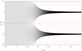
Figure 1: Solid black curves show numerical solutions of equation (28) for $\alpha=0.5$, $\beta=1$. The separatrix is shown dashed. The red dotted curves show contours of the pressure, with the red dashed curve being the one at $p=0$ which passes through the apex of the bubble.

Possible solutions of this equation must satisfy the boundary conditions at $x\to\pm\infty$, periodicity, and the requirement that the line $p=0$ must be a streamline. If we initially neglect the last of these requirements, a fairly broad class of solutions is possible, functions with branch cuts and poles placed periodically and symmetrically within the bubbles. We will study the results of using the simplest of these

$$v_{x}=\alpha+\beta\ln(1+\exp x),$$ (24)

where $\beta$ is an arbitrary dimensionless constant, which has been chosen to tend to the usual exponential decay of perturbation velocity as $x\to-\infty$ but increase linearly as $x\to\infty$. This form can be related to the conformal transformation applied by Duchemin et al. in their study of the asymptotic spike dynamics in Atwood number unity Rayleigh-Taylor instability.Duchemin, Josserand, and Clavin (2005)

Equation (24) can be integrated in $x$ and analytically continued to give $\varphi=\alpha z-\beta{\rm Li}_{2}(-\exp z)$, where ${\rm Li}_{2}$ is the dilogarithm

$${\rm Li}_{2}(z)=\sum_{k=1}^{\infty}{z^{k}\over k^{2}}=-\int_{0}^{z}{\ln(1-u)\over u}{\rm\,d}u.$$ (25)

The power series expansion means that the potential can be considered as a particular form of the multiple harmonic expansionAbarzhi, Glimm, and Lin (2003); Sohn (2012), chosen to have acceptable behaviour at $x\to\infty$ to allow for the behaviour of the spikes. However, the appearance of a branch cut within the excluded flow gives the solution a rather distinct character.

Differentiating this analytic function again gives the velocity distribution

$$v_{x} = \alpha+{\beta\over 2}\ln\left[1+2\cos(y)\exp(x)+\exp(2x)\right]$$ (26)

$$v_{y} = -\beta\arctan\left[\sin y\over\cos y+\exp(-x)\right].$$ (27)

We can choose that the branch cut for $x>0$, lies on the lines $y=(2n+1)\pi$, where $v_{y}$ is no longer continuous, so that this branch cut resides within the void region separating the jets. Streamlines within the void region will not be continuous with $x\to-\infty$.

An ordinary differential equation for the streamlines may be derived by dividing equation (27) by equation (26)

$${{\rm d}y\over{\rm d}x}={-\arctan\left[\sin y/\left(\cos y+\exp(-x)\right)\right]\over(\alpha/\beta)+{1\over 2}\ln\left[1+2\cos(y)\exp(x)+\exp(2x)\right]},$$ (28)

which demonstrates that the streamlines are determined by $\alpha/\beta$. Some numerical solutions of this equation are shown in Figure 1. We have confirmed that these solutions are coincident with the contours of ${\rm I}m(\varphi)$. We evaluate the dilogarithm function using the methods described by Vollinger & Weinzierl.Vollinga and Weinzierl (2005)

The values of the dimensionless parameters $\alpha$ and $\beta$ may be constrained by considering the boundary conditions at the apex of the bubble, where $y=\pm\pi$, and $v_{x}=p=0$. The apex is at $x_{a}$, which must satisfy $v_{x}(x_{a}+i\pi)=0$, i.e.

$$1-\exp x_{a}=\exp-\alpha/\beta,$$ (29)

and

$$v_{y}=-\beta\arctan\left[1-\exp\left(-\alpha/\beta\right)\right].$$ (30)

The boundary condition $p=0$ must be satisfied along the full surface of the jet. It would be possible to constrain the lowest harmonic solution further by solving for the curvature at the head of the bubble, which could be done by using equations (21) and (22) to derive an expression for $v\cdot\nabla p$, which must be zero close to the apex. However, given the global nature of the solution, there is a trade-off between the accuracy of the approximation at the head of the bubble and at larger distances. We will illustrate the results for values chosen to give acceptable accuracy overall.

In Figure 1, we include pressure contours derived using equation (23). For the values which we have chosen, the pressure contour through the apex lies close to the surface streamline for a significant distance around the bubble. Varying $\alpha$ and $\beta$ allows the contours at $x\to\infty$ to be made more closely parallel to the surface, at the cost of reducing the accuracy of the fit to the bubble.

V Comparison with flow simulation

We base our calculations on the shock conditions used by Cherne et al.Cherne et al. (2015) They model a shocked copper surface, assuming that the copper is a perfect fluid with $\gamma=3.0$ and density $8.93{\rm\,g\,cm^{-3}}$, with a light fluid ahead of it with $\gamma=5/3$ and density $1.22\times 10^{-3}{\rm\,g\,cm^{-3}}$. The impinging shock is taken to have Mach number $2.5$. To obtain a post-shock pressure consistent with their results, the ambient pressure is assumed to be $10^{5}{\rm\,Pa}$, while the shocked gas pressure is $8.875\times 10^{5}{\rm\,Pa}$. We have confirmed that this gives the shocked density and release density given in section IIIB of this paper. We offset the frame of motion of our calculations by $403.6{\rm\,cm\,s^{-1}}$ so that an unperturbed shocked interface would be at rest. The timescales reported are scaled to a characteristic growth time, which we will denote as $\tau^{\star}$ to distinguish it from the self-similar scaling timescale which is expected to be similar, but may not be identical. This is defined as $\tau^{\star}=\lambda/(3\pi\dot{\eta}_{0}^{b})$, where $\dot{\eta}_{0}^{b}=F_{l}F_{nl}^{b}|kh_{0}\Delta u|$, with $F_{l}=1-\Delta u/2u_{s}$ and $F_{nl}^{b}=1/(1+kh_{0}/6)$. $h_{0}$ is the initial amplitude of the surface perturbations, $u_{s}$ is the shock velocity, and $\Delta u$ is the velocity jump of the interface; $F_{l}$ allows for the effect of the compression of the initial amplitude, while $F_{nl}^{b}$ models the saturation of the bubble velocity at large initial amplitudes.

These calculation presented here have been made with the finite-difference fluid dynamics code TURMOILYoungs (1991). This code is particularly suited for this study, as a result of its good performance in the low Mach number limit, for flows such as single-mode Kelvin-Helmholtz roll-upThornber et al. (2008). The TURMOIL code also implements semi-Lagrangian mesh motion and one-dimensional Lagrangian boundary regions, which we use to allow the mesh to move with the mean material velocity, and hence to minimize advective dissipation.

We concentrate on the low initial amplitude case $kh_{0}=1/8$ to minimize jetting from the apex of the bubbleCherne et al. (2015), which can be driven by post-shock reverberations in the dense material. As in this previous work, the calculations presented have been run with a lateral resolution of 256 cells per wavelength, and with a large domain size in the direction of shock propagation to avoid boundary effects: this requires particular care for these calculations, as a result of the high sound speed in the more diffuse gas.

We have also included passively-advected tracer value in the calculations, with an initial value set by the lateral coordinate value of the cell. This allows us to infer the approximate origin of the material in each cell at later time. The growth of the interfacial area with time is determined by a combination of a smooth straining of the material on the original interface, and the appearance of new surface material at the apex of the bubble. In Figure 3, we see that the initial surface material has for the most part been advected into the spike. As Kelvin’s theorem implies that vorticity is advected with the material, the memory of the detail of the initial surface profile which determined the vorticity deposition is also carried into the spike. Hence, as has been observed elsewhere,Cherne et al. (2015) differing surface profiles will lead to changes in the detailed structure of the spike tip, but the bubble shape will tend to become universal at late time.

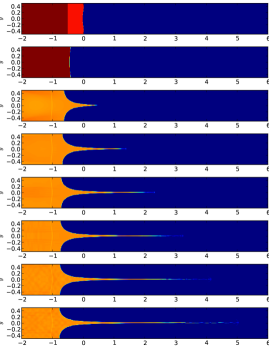
Figure 2: Density evolution for a $kh_{0}=1/8$ sinusoidal initial perturbation. The top figure is the initial condition, and subsequent frames are at $t/\tau^{\star}=0,1,2,3,4,5,6$. The narrow band of low density material at $x=-1$ is caused by a small entropy spike deposited at the initial shock position.

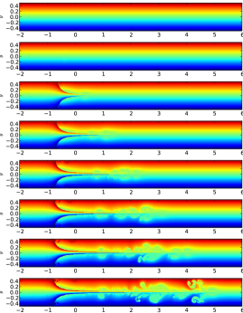
Figure 3: Evolution of a tracer variable set to the initial $y$ position for a $kh_{0}=1/8$ sinusoidal initial perturbation. The top figure is the initial condition, and subsequent frames are at $t/\tau^{\star}=0,1,2,3,4,5,6$.

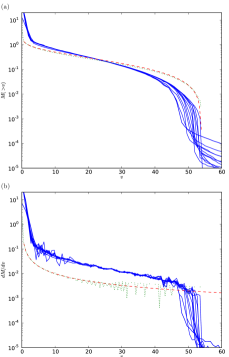
Figure 4: Mass-velocity plots from calculations: (a) cumulative, (b) resolved. Blue curves show the calculation results (the knee in these curves at high velocity, corresponding to the tip of the spike, decelerates somewhat with time). Dashed red curves show the simple model of equation (8), and dotted green curves the similarity solution shown in Figure 1 (which is subject to numerical noise, as a result of spatial sampling of the solution). Relative normalizations are arbitrary.

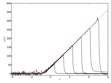
Figure 5: Comparison of the flow velocity along the axis of the jet scaled into similarity units, $v_{x}t/\tau^{\star}$ (solid curves), with the axial velocity given by equation (24), in the frame of the upstream material (dashed red curve). The fluctuations in velocity ahead of the spike at the latest times are due to the start of vortex shedding from the tip.

In Figure 2 we show the evolution of the material density with time. The shape of the bubble is seen to converge to a form very similar to that of the asymptotic solution in Figure 1. Figure 3 shows the evolution of the tracer variable set equal to the initial $y$ position of the material. As the flow converges, the contours on this plot will tend to streamlines of the flow. It can be seen that at late time the majority of the material on the spike surface has passed through the stagnation point at the head of the bubble, so information on the initial surface form encoded by the initial surface vorticity field will have been advected into the spike.

Vortical structures are seen to develop in the low-density material, as a result of Kelvin-Helmholtz instability at the surface of the spike, and at the head of the bubble. At later times than shown here, a small spike appears at the head of the bubble, breaking the self-similar convergence. This is a familiar phenomenon seen in previous calculations.Cherne et al. (2015) It is worth noting, however, that the decaying stagnation flow at the bubble head is also likely to be particularly liable to the carbuncle phenomenon.Quirk (1994)

In Figure 4(a), we compare the cumulative mass determined from the calculations to the simple model of equation (8). Several timesteps are plotted on this image, which demonstrates that the mass-velocity distribution has essentially converged by the first timestep shown, $t/\tau^{\star}=1$. The convergence is more rapid than that suggested by equation (1), presumably because we have included the mass of all material in the calculation in our evaluation of $M(>v)$, rather than just the material which has moved beyond the mean free surface. The model curve is defined by the maximal velocity and overall scale. The model distribution has a similar form to the calculational data. The numerical accuracy of the fit is not great; however, the details of the distribution at the spike tip are expected to be dependent on the initial surface profile. The velocity-resolved plot shown in Figure 4(b), while more noisy, confirms that mass-velocity distribution in the similarity solution agrees well with the analytical form equation (8). The comparison with the results of the numerial calculation suggests the disagreement in Figure 4(a) is primarily the result of the structure at the tip of the spike.

In Figure 5, we compare the speed along the axis of the jet scaled into similarity units, $v_{x}t/\tau^{\star}$. This plot demonstrates the self-similar collapse of the calculation results very well, with very minor scatter resulting from acoustic modes in the material upstream of the bubble. The level of agreement with the axial velocity given by equation (24) here is also very good, from the bulk material as far as the tip of the spike.

VI Conclusions

In the present paper, we have derived a self-similar theory for the asymptotic behaviour of high density contrast, single-mode Richtmyer-Meshkov instability. To match the behaviour of the spikes at large distances, we have assumed an alternative (but related) form of velocity potential to that considered in previous studies. We propose a simple form for the mass-velocity relationship in the spikes, equation (8), which fits the behaviour seen in calculations to good accuracy, and a more detailed approximate form for the velocity throughout the dense material, equations (26) and (27). In contrast to most previous studies of Richtmyer-Meshkov instability, we model the late-time asymptotic behaviour of the dense material as a single domain, rather than treating the bubble or spike in isolation.

As noted above, Abarzhi et al.Abarzhi, Glimm, and Lin (2003) used a multiple harmonic expansion to avoid the appearance of a mass flux at infinity in their model for RT instability. The potential we assume includes a mass flux at infinity, but has a similar character to that considered by Abarzhi et al., in that it has been chosen to match the asymptotic behaviour of Richtmyer-Meshkov spikes at Atwood number unity, rather than being exponentially divergent.

The work has focussed upon the growth of two dimensional, single mode perturbations at high Atwood number. The development of a general surface will combine features of the behaviour for regular perturbations and with those for a localized axisymmetric perturbations: a localized source at an interface will have a different scaling behaviourArthur and Falle (1991).