Bayesian Non-Exhaustive Classification
A Case Study: Online Name Disambiguation using Temporal Record Streams  

Abstract

The name entity disambiguation task aims to partition the records of multiple real-life persons so that each partition contains records pertaining to a unique person. Most of the existing solutions for this task operate in a batch mode, where all records to be disambiguated are initially available to the algorithm. However, more realistic settings require that the name disambiguation task be performed in an online fashion, in addition to, being able to identify records of new ambiguous entities having no preexisting records. In this work, we propose a Bayesian non-exhaustive classification framework for solving online name disambiguation task. Our proposed method uses a Dirichlet process prior with a Normal $\times$ Normal $\times$ Inverse Wishart data model which enables identification of new ambiguous entities who have no records in the training data. For online classification, we use one sweep Gibbs sampler which is very efficient and effective. As a case study we consider bibliographic data in a temporal stream format and disambiguate authors by partitioning their papers into homogeneous groups. Our experimental results demonstrate that the proposed method is better than existing methods for performing online name disambiguation task.

1 Introduction

Name entity disambiguation [13, 14, 27, 32] (also known as name entity resolution) is an important problem, which has numerous applications in information retrieval [24, 7], digital forensic [20], and social network analysis [30, 6, 19]. In information retrieval domain, name disambiguation is important for sanitizing search results of ambiguous queries. For example, an online search query for “Michael Jordan” may retrieve pages of former US basketball player, the pages of UC Berkeley machine learning professor, and the pages of other persons having that name, and name disambiguation is needed to organize those pages in homogeneous groups. In digital forensic, resolving name ambiguity is essential before inserting a person’s profile in a law enforcement database; failing to do so may cause severe distress to many innocents who are namesakes of a known criminal. Evidently, name disambiguation plagues the digital library science domain the most. In this domain, a key task is to record academic publications in digital repositories and it is often the case that the publications of multiple scholars sharing a name are recorded erroneously under a unique profile in some repositories. For example, in Google Scholar (GS), which is one of the largest digital libraries for scholarly publications from various disciplines, there are more than $50$ distinct persons named “Wei Wang”, all of whose publications are listed under the same entity. Severe cases of name ambiguity like this arise in digital library because the first name of an author is typically written in an abbreviated form in the citation of many scientific articles. Unresolved name ambiguity in digital library over- or under-estimates a scholar’s citation related impact metrics.

Due to its importance, the task of name entity disambiguation has allured data mining and database researchers, and over the years, they have proposed several methods for solving this problem [4, 13]. The proposed methodologies differ in their learning approaches (supervised [13] or unsupervised [14] [5]), machine learning methodologies (support vector machines [13], Markov random field [27], graph clustering [14], etc) and the data sources that they use (internal data or external data, such as Wikipedia [4]). Many of the proposed methods are specific to resolving name ambiguity in digital library, and the major contribution in these works is effective feature engineering involving co-authors, publication venues, and research keywords. However, a key limitation of most of the existing methods for name disambiguation is that they operate in a batch mode, where all records to be resolved are initially accessible to the learning algorithm and a learning model is trained using features extracted from these records. Hence, they fail to resolve emerging name ambiguities caused from the evolution of digital data, or they fail to utilize emerging evidences suggestive of merging of name entities which are separated in the existing state. Re-running a batch learning to catch up with the data evolution is not practical due to the enormity of the computation on a large digital repository. So, it is more practical to perform name entity disambiguation task in an incremental fashion by considering the streaming nature of records. We call this online name entity disambiguation, which is the focus of this work.

Perhaps, the most prudent among the existing name disambiguation methodologies is supervised classification where for a given name reference  a classification model is trained which classifies each of the records into a given number of entities (sharing that name). However, such a method is unable to identify records belonging to emerging name entities, who do not have any record in the training data. For example, in digital library, every now and then, papers are authored by a new scholar who is a namesake of some of the existing scholars; as an example, consider the name reference “Lei Wang" in Arnetminer  bibliographic data repository. In 1999, there were a handful of authors sharing that name, but with each passing year this number has been growing and in 2010 there existed more than 100 authors that have that same name (See Figure 1). A supervised classification model for the name reference “Lei Wang”, with a fixed number of classes will never be able to disambiguate the papers of new authors correctly, as these models have no provision for inclusion of new classes instantly.

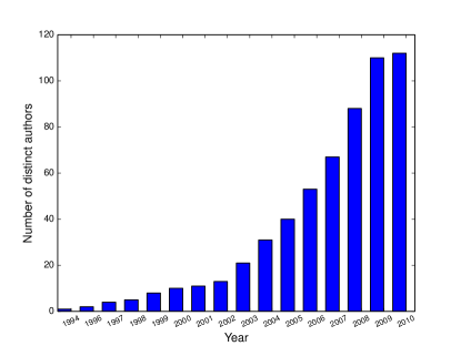
Figure 1: Name Ambiguity Evolution for the case of “Lei Wang"

Majority of the existing works on name entity disambiguation consider batch learning solution, however, very recently online name disambiguation is gaining some traction with a few works [22, 17, 9, 28]. However, all of these methods propose a threshold-based approach for identifying emerging classes with a heuristically chosen threshold leading to unpredictable performance. Real-life online digital library platforms, such as ResearchGate , confirm the authorship of ambiguous records with the authors themselves before including them in their profiles. However, such a solution may not be very effective as it relies on a manual verification process which is tedious, and also introduces significant indexing delays for new records.

In this work, we solve the online name disambiguation task by a principled approach, namely Bayesian non-exhaustive classification framework. We use non-exhaustive learning [10, 21] —a recent development in machine learning, which considers the scenario that training data may miss some classes; it enables our proposed method to disambiguate records belonging to not only the existing entities, but also the emerging ones. Specifically, given a non-exhaustive training dataset, we use a Dirichlet process prior to model both known and emerging classes, where each class distribution is modeled by a Normal distribution. We use a common Normal $\times$ Inverse Wishart (NIW) prior to model the mean vectors and covariance matrices of all class distributions. The hyperparameters of the NIW prior are estimated using data from known classes facilitating information sharing between known and emerging classes. For a future record, the proposed approach computes class conditional probabilities by considering the possibility that the record may also originate from a new class. Based on these probabilities each record is assigned to one of the existing classes, or to an emerging class that has no previous records in the training set. We update the set of classes every time a new class is created by the online model and then use a new classification model to classify subsequent records. The proposed framework paves the way for simultaneous online classification and novel class discovery.

Our contributions can be summarized as follows:

1. We study online name disambiguation problem in a non-exhaustive streaming setting and propose a self-adjusting Bayesian model that is capable of performing classification, and class discovery, at the same time. To the best of our knowledge, our work is the first one to adapt Bayesian non-exhaustive learning for online name disambiguation task.

2. We propose a one sweep Gibbs sampler to perform online non-exhaustive classification in order to efficiently evaluate the class assignment of an online record.

3. We demonstrate the utility of our proposed approach on bibliographic datasets and present experimental results, which demonstrate the superiority of our proposed method over the state-of-the-art methodologies for online name disambiguation.

2 Related Work

There exist a large number of works on name entity disambiguation. In terms of methodologies, supervised [4, 13], unsupervised [14, 5], and probabilistic relational models [27, 29, 26], are considered. In a supervised setting, a distinct entity can be considered as a class, and the objective is to classify each record to one of the classes. Han et al. [13] propose supervised name disambiguation methodologies by utilizing Naive Bayes and SVM for name entity disambiguation task. For unsupervised name disambiguation, the records are partitioned into several clusters with the goal of obtaining a partition where each cluster contains records from a unique entity. For example,  [14] proposes one of the earliest unsupervised name disambiguation methods for bibliographical data, which is based on $K$-way spectral clustering. Specifically, they compute Gram matrix representing similarities between different citations and apply $K$-way spectral clustering algorithm on the Gram matrix in order to obtain the desired clusters of the citations. Recently, probabilistic relational models, especially graphical models have also been considered for the name entity disambiguation task. For instance, [27] proposes to use Markov Random Fields to address name entity disambiguation challenge in a unified probabilistic framework. Another work is presented in  [29] which uses pairwise factor graph model for this task.  [32, 23, 15] present approaches for the name disambiguation task on anonymized graphs and they only leverage graph topological features due to the privacy concerns. In addition,  [31] solves name entity disambiguation problem as the privacy-preserving classification task such that the anonymized dataset satisfies non-disclosure requirements, at the same time it achieves high disambiguation performance.

Most of existing methods above tackle disambiguation task in a batch setting, where all records to be resolved are initially available to the algorithm, which makes them unsuitable for disambiguating a future record. In recent years, a few works have considered online name entity disambiguation [22, 17, 28, 9, 8, 16], which perform name disambiguation incrementally without retraining the system every time a new record is received. Khabsa et al. [17] use an online variant of DBSCAN, a well-known density-based clustering to cluster new records incrementally as they are being added. Since, DBSCAN does not take the number of clusters as input, technically speaking, this method is able to adapt to the non-exhaustive scenario simply by assigning a new record in a new cluster, as needed. However, DBSCAN is quite susceptible to the choice of parameter values, and depending on the parameter value, a record belonging to an emerging class can simply be labeled as an outlier instance.  [22] proposes a two stage framework for online name disambiguation. The first stage performs batch name disambiguation to disambiguate all the records no later than a given time threshold using hierarchical agglomerative clustering. The second stage performs incremental name disambiguation to determine the class membership of a newly added record. However, the method uses a heuristic threshold to decide on the cluster assignments of new records which makes this approach very susceptible to the choice of threshold parameter.  [28] introduces an association rule based approach for detecting unseen authors in test set. However, the major drawback of proposed solution is that it can only identify records of emerging authors in a binary setting but fails to further distinguish among them.  [8] presents the Expectation Maximization based approach for the name disambiguation in Twitter streaming data. In addition,  [16] proposes a threshold based method to discover emerging entities with ambiguous names in the domain of knowledge base.

Our proposed solution utilizes non-exhaustive learning—a rather recent development in machine learning.  [1, 10, 21] are some of the existing works related to non-exhaustive learning. Akova et al. [1] propose a Bayesian approach for detecting emerging classes based on posterior probabilities. However, the decision function for identifying emerging classes uses a heuristic threshold and does not consider a prior model over class parameters; hence the emerging class detection procedure of this model is purely data-driven. Miller et al.  [21] present a mixture model using expectation maximization (EM) for online class discovery.  [10] proposes a sequential importance sampling based online inference approach for emerging class discovery and the work is motivated by a bio-detection application.

3 Problem Formulation

For a given name reference $a$, assume $X_{n}$ is a stream of records associated with $a$. The subscript $n$ represents the identifier of the last record in the stream and the value of this identifier increases as new records are observed in the stream. Each record $x_{i}\in X_{n}$ can be represented by a $d$-dimensional vector which is the feature representation of the record in a metric space. In real-life, the name reference $a$ is associated with multiple persons (say $k$) all sharing the same name, $a$. The task of name entity disambiguation is to partition $X_{n}$ into $k$ disjoint sets such that each partition contains records of a unique person entity. When $k$ is fixed and known a priori, name entity disambiguation can be solved as a $k$-class classification task using supervised learning methodologies. However, for many domains the number of classes ($k$) is not known, rather with new records being inserted in the stream, $X_{n}$ , the number of distinct person entities associated with $a$ may increase. The objective of online name entity disambiguation is to learn a model that assigns each incoming record into an appropriate partition containing records of a unique person entity.

Online name entity disambiguation is marred by several challenges, which we discuss below:

First, for a given record stream $X_{n}=\{x_{1},\cdots,x_{i},\cdots,x_{n}\}$, the record $x_{i}$ is classified with the records leading up to $x_{i-1}$, i.e. $X_{i-1}$ is our training data for this classification task. However, the record $x_{i}$ may belong to a new person entity (having name $a$) with no previous records in $X_{i-1}$. This happens because for online setting, the number of real-life name entities in $X_{n}$ is not fixed, rather it increases over the time. A traditional $k$-class supervised classification model which is trained with records of known entities mis-classifies the new emerging record with certainty, leading to an ill-defined classification problem. So, for online name entity disambiguation, a learning model is needed which works in non-exhaustive setting, where instances of some classes are not at all available in the training data. In existing works, this challenge is resolved using clustering framework where a new cluster is introduced for the emerging record of a new person entity, but this solution is not robust because small changes in clustering parameters make widely varying clustering outcomes.

The second challenge is that online name entity disambiguation, more often, leads to a severely imbalanced classification task. This is due to the fact that in most of the real-life name entity disambiguation problems, the size of the true partitions of the record set $X_{n}$ follows a power-law distribution. In other words, there are a few persons (dominant entities) with the name reference $a$ to whom the majority of the records belong. Only a few records (typically one or two) belong to each of the remaining entities (with name reference $a$). Typically, the persons whose records appear at earlier time are dominant entities, which makes identifying novel entity an even more challenging task.

The third challenge in online name entity disambiguation is related to online learning scenario, where the incoming record is not merely a test instance of typical supervised learning. Rather, the learning algorithm requires to detect whether the incoming record belongs to a novel entity, and if so, the algorithm must adapt itself and configure model to identify future records of this novel entity. Overall, this requires a self-adjusting model that updates the number of classes to accurately classify incoming records of both new and existing entities.

The final challenge in our list is related to temporal ordering of the records. In traditional classification, records do not have any temporal connotation, so an arbitrary train/test split is permitted. But, for online setting the model must respect time order of the records, i.e., a future record cannot be used for building a training model that classifies as older record.

Our proposed model overcomes all the above challenges by using a principled approach.

4 Entity Disambiguation on Bibliographic Data

As we have mentioned earlier, name entity disambiguation is a severe issue in digital library domain. In many other domains, solving name disambiguation is easier as the method may have access to personalized attributes of an entity, such as institution affiliation, and email address. But, in digital library, the reference of a paper only includes paper title, author name, publication venue, and year of publication, which are not sufficient for disambiguation of most of the name references. Besides, in many citations the first name of the authors are often replaced by initials, which worsen the disambiguation issue. As a result, nearly, all the online bibliographic repositories, including DBLP, Google scholar, ArnetMiner, and PubMed, suffer from this issue. Nevertheless, these repositories provide timely update of the publication data along with their chronological orders, so they provide an ideal for evaluating the effectiveness of an online name entity disambiguation method.

In this work, we use bibliographic data as a case study for online name entity disambiguation. For each name reference $a$, we build a distinct classification model. The record stream $X_{n}$ for the name reference $a$ is the chronologically ordered stream of scholarly publications where $a$ is one of the authors. To build a feature vector for a paper in $X_{n}$ we extract features from its author-list, keywords from its paper title, and paper venue (journal/conference). We provide more details of feature construction in the following subsection.

4.1 Feature Matrix Construction and Preprocessing

For a given name reference $a$, say we have a record stream containing $n$ papers for which the name reference $a$ is in the author-list. We represent each paper with a $d$ dimensional feature vector. Then we define a data matrix $X_{n}\in{\rm I\!R}^{n\times d}$ for $a$, in which each row corresponds to a record (paper) and each column represents a feature . In addition, each paper has a class label $l_{i}$ representing the $i$-th distinct person entity under name reference $a$, who has authored this paper. Our goal is to learn a model to partition papers with name reference $a$ in an online setting.

For a paper, we construct its feature vector (a row of matrix $X_{n}$) using author information, paper title, and publication venue as attributes. These features are well-known for name disambiguation in digital library. For author information, we first aggregate the author-list of all papers into authors, then define a binary feature representation for each author, indicating his presence or absence in the author-list of that paper. For constructing keyword based feature, we first filter a set of predefined stop words from the paper titles and use the remaining words as a feature. For a given paper, we use a binary value based on presence or absence of that word in the title of that paper. Publication venues are converted to binary feature in the same way. For keywords, instead of using binary value, we have also considered TF-IDF value, but it does not provide noticeable performance improvement in any of our datasets. A possible reason for that could be we pre-process the data matrix with dimensionality reduction, which is able to capture hidden features directly from a binary data matrix.

Dimensionality reduction step reduces the dimensionality of data matrix $X_{n}\in{\rm I\!R}^{n\times d}$. This step is important because the matrix $X_{n}$ is severely sparse with many zero entries. For dimensionality reduction we design an incremental variant of Non-Negative Matrix Factorization (INNMF), which maps $X_{n}$ into a low dimensional space denoted as $E_{n}\in{\rm I\!R}^{n\times h}$, where $h$ is the number of hidden dimensions . Specifically, we first perform Non-Negative Matrix Factorization (NNMF) [18] in the batch mode on the set of training records initially available. Then in the online mode, we express each sequentially observed record by a linear combination of the basis vectors generated from initial set of training records, where the coefficients of the basis vectors serve as our latent feature values. In order to learn the coefficients, we solve a constrained quadratic programming problem by minimizing a least square loss function under the constraint that each coefficient is non-negative. The goal of using INNMF is to discover low dimensional latent features for each sequentially observed record in an effort to better fit our proposed Normal $\times$ Normal $\times$ Inverse Wishart (NNIW) data model.

After pre-processing, low dimensional data matrix $E_{n}$ is a collection of time-stamped $n$ record streams with which $a$ is associated, namely $E_{n}=\{e_{1},...,e_{i},...,e_{n}\}$, where $e_{i}\in{\rm I\!R}^{1\times h}$ is a $h$ dimensional row vector generated from INNMF to represent the $i$-th record in the given temporal record stream, and all of the $n$ records in $E_{n}$ are sorted temporally, namely $e_{1}.t\leq...\leq e_{i}.t\leq...\leq e_{n}.t$, where $e_{i}.t$ represents the time for record $e_{i}$.

By using an incessant stream of records, we formalize our online name disambiguation task as follows: given a time-stamped partition $t_{0}$, we consider two types of records, namely record samples initially available in the training set with known class membership information, and record samples sequentially observed online with no verified class membership information. Formally we treat the collection of time-stamped record streams $E_{n}=\{e_{1},...,e_{i},...,e_{n}\}$ as the set of training samples initially available, where $e_{1}.t\leq...\leq e_{n}.t\leq t_{0}$ and $n$ is the total number of samples in $E_{n}$. As we can see, all of the records in $E_{n}$ occur no later than the given time-stamped threshold $t_{0}$. $Y_{n}=(y_{1},...,y_{i},...,y_{n})$ is class indicator vector with $y_{i}\in\{l_{1},..,l_{k}\}$, where $k$ is the number of distinct classes in the training set. In order to differentiate records in the training set from those observed online, we use $\tilde{e}_{i}\in{\rm I\!R}^{1\times h}$ to represent $i$-th record sequentially observed online. Here we define $\tilde{E}_{r}=\{\tilde{e}_{1},...,\tilde{e}_{i},...,\tilde{e}_{r}\}$ to be the set of $r$ record samples sequentially available online after time threshold $t_{0}$, i.e. $t_{0}\leq\tilde{e}_{1}.t\leq...\leq\tilde{e}_{r}.t$. As new ambiguous authors emerge with the incoming records, the set of classes may expand. Here we denote $\tilde{Y}_{r}=(\tilde{y}_{1},...,\tilde{y}_{i},...,\tilde{y}_{r})$ to be their corresponding unknown class information with $\tilde{y}_{i}\in\{l_{1},...,l_{\tilde{k}_{r}+k}\}$, where $\tilde{k}_{r}$ is the number of new classes associated with these $r$ records observed online.

Given an arbitrary online record $\tilde{e}\in{\rm I\!R}^{1\times h}$ at a certain time point, our proposed Bayesian non-exhaustive classification model computes a probability to decide whether we should assign $\tilde{e}$ to one of the existing classes, or to a new class not yet observed in any of the historical records.

5 Method

In this section we discuss Bayesian non-exhaustive name entity disambiguation methodologies. The methodologies discussed in this section are domain neutral and can be applied to any domain, once an appropriately constructed feature matrix is obtained.

5.1 Dirichlet Process Prior Model

We model the set of record streams $E_{n}=\{e_{1},...,e_{n}\}$ by using a set of latent parameters $\{\theta_{1},...,\theta_{n}\}$. Each $\theta_{i}$ is drawn independently and identically (iid) by a Dirichlet Process [11] (DP), while each record $e_{i}\in{\rm I\!R}^{1\times h}$ is distributed according to an unknown distribution $F(\theta_{i})$ parametrized by $\theta_{i}$. Mathematically,

$$G \sim DP(\alpha,H)$$

$$\theta_{i} \sim G$$

$$e_{i}|\theta_{i} \sim F(\theta_{i})$$

where $G$ is a random discrete probability measure defined by a base distribution $H$ along with the precision parameter $\alpha>0$.

It is a common practice to use stick breaking construction [25] to represent samples drawn from a Dirichlet process as below:

$$\phi_{i} \sim H$$

$$\beta_{i} \sim Beta(1,\alpha)$$

$$\pi_{i} = \beta_{i}\prod_{j=1}^{i-1}(1-\beta_{j})$$

As shown in Equation 5.1, in order to simulate the process of stick breaking construction, imagine we have a stick of length $1$ to represent total probability. We first generate each point $\phi_{i}$ from base distribution $H$, which originates from our proposed NNIW data model (Details in Section 5.4). Then we sample a random variable $\beta_{i}$ from Beta(1, $\alpha$) distribution. After that we break off a fraction $\beta_{i}$ of the remaining stick as the weight of parameter $\phi_{i}$, denoted as $\pi_{i}$. In this way it allows us to represent random discrete probability measure $G$ as a probability mass function in terms of infinitely many $\phi_{1},...,\phi_{\infty}$ and their corresponding weights $\pi_{1},...,\pi_{\infty}$ yielding $G=\displaystyle\sum_{i=1}^{\infty}\pi_{i}\delta_{{\phi_{i}}}$, where $\delta_{{\phi_{i}}}$ is the point mass of $\phi_{i}$.

5.2 Bayesian Non-Exhaustive Online Classification

Consider that at a certain time point, we have a set of $n$ training records for name reference $a$, denoted by $E_{n}=\{e_{1},...,e_{n}\}$ where each record is assigned to a latent parameter from the set $\{\theta_{1},...,\theta_{n}\}$. A future online record $\tilde{e}$ is assigned to $\tilde{\theta}$ with a probability

$$\tilde{\theta}|\theta_{1},...,\theta_{n}\sim\frac{\alpha}{\alpha+n}H+\frac{1}{\alpha+n}\sum_{i=1}^{n}\delta_{\theta_{i}}$$ (3)

The conditional prior distribution in Equation 3 can be interpreted by a mixture of two distributions. Specifically, given the future record $\tilde{e}$ with parameter $\tilde{\theta}$, $\tilde{e}$ belongs to the base distribution $H$ with probability $\frac{\alpha}{\alpha+n}$ and it originates from random discrete probability measure $G$ generated from DP with probability $\frac{n}{\alpha+n}$. Since $G$ is a discrete distribution, each record in a sequence of $n$ records generated from $G$ may not belong to a distinct $\theta_{i}$. If we assume that there are $k$ distinct values of $\theta$ associated with the first $n$ records, then we can re-write Equation 3 as below:

$$\tilde{\theta}|\theta_{1},...,\theta_{n}\sim\frac{\alpha}{\alpha+n}H+\frac{1}{\alpha+n}\sum_{j=1}^{k}n_{j}\delta_{\theta_{j}}$$ (4)

where in the last expression of Equation 4, $\theta_{j}$ represents each distinct $\theta$, and $n_{j}$ denotes the number of times $\theta_{j}$ appears among the sequence of $n$ records. Furthermore, each $\theta_{j}$ is associated with a unique class $l_{j}$ whose corresponding record $e_{j}$ is generated according to $F(\theta_{j})$. Thus after a sequence of $n$ records are observed, $\tilde{y}$, the class membership of the future record $\tilde{e}$, is equal to $l_{j}$ with probability $\frac{n_{j}}{\alpha+n}$, and it is equal to $l_{k+1}$ with probability $\frac{\alpha}{\alpha+n}$, where $l_{k+1}$ is an emerging class which has not been observed in the sequence of $n$ training records.

Next we incorporate the data model into the Dirichlet process prior and use the conditional posterior to determine whether $\tilde{e}$ should be assigned to one of the existing classes or to an emerging class. More specifically, we are interested to evaluate the following distribution:

$$p(\tilde{\theta}|\tilde{e},\theta_{1},...,\theta_{n})$$

$$\propto \frac{\alpha}{\alpha+n}p(\tilde{e})p(\tilde{\theta}|\tilde{e})$$

$$+ \frac{1}{\alpha+n}\displaystyle\sum_{j=1}^{k}n_{j}p(\tilde{e}|\theta_{j})\delta_{\theta_{j}}$$

As we can observe from Equation 5.2, $\tilde{e}$ either belongs to a new class $l_{k+1}$ with the probability proportional to $\frac{\alpha}{\alpha+n}p(\tilde{e})$, or to a existing class $l_{j}$ with the probability proportional to $\frac{n_{j}}{\alpha+n}p(\tilde{e}|\theta_{j})$.

Due to the fact that $\theta_{j}$ is not known for online record sequence, here we replace $p(\tilde{e}|\theta_{j})$ with the conditional predictive distribution $p(\tilde{e}|D_{j})$, where $D_{j}=\{e_{i}\}_{i\in l_{j}}$ represents the subset of records with class label $l_{j}$. Thus for the online record $\tilde{e}$, given the class membership information of all of $n$ sequence of records processed before $\tilde{e}$, the following decision making function $g(\tilde{e})$ decides whether $\tilde{e}$ belongs to an emerging class or to one of the existing ones.

$$g(\tilde{e})=\begin{cases}\tilde{y}=l_{j^{\ast}},&\text{if }\\ \frac{n_{j^{\ast}}}{\alpha+n}p(\tilde{e}|D_{j^{\ast}})\geq\frac{\alpha}{\alpha+n}p(\tilde{e})\\ \tilde{y}=l_{k+1},&\text{if }\\ \frac{n_{j^{\ast}}}{\alpha+n}p(\tilde{e}|D_{j^{\ast}})<\frac{\alpha}{\alpha+n}p(\tilde{e})\end{cases}$$ (6)

where $j^{\ast}=argmax_{j}\left\{\frac{n_{j}}{\alpha+n}p(\tilde{e}|D_{j})\right\}_{j=1}^{k}$.

5.3 Gibbs Sampler for Non-Exhaustive Learning

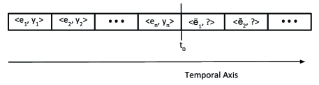
Figure 2: Demonstration of Temporal Record Stream

As shown in Figure 2, since we only have access to the class membership information $Y_{n}$ for the streaming records initially available in the training set $E_{n}$, which occur no later than the given time-stamped threshold $t_{0}$, and the class membership $\tilde{Y}_{i-1}=(\tilde{y}_{1},\cdots,\tilde{y}_{i-1})$ of online sequentially observed record stream $\tilde{E}_{i-1}=\{\tilde{e}_{1},\cdots,\tilde{e}_{i-1}\}$ is not verified, thus it is impractical to evaluate the decision function shown in Equation 6 directly. Instead in order to respect the temporal order of each record, we utilize one sweep Gibbs sampler for online classification to efficiently evaluate the probability of an online record belonging to an emerging class or to one of the existing ones. If $\tilde{y}_{i}$ is the predicted class label of $i$-th online observed record $\tilde{e}_{i}$, the conditional distributions of the class indicator variable $\tilde{y}_{i}$ can be easily obtained via one sweep Gibbs sampler. Specifically, we are interested to sample from the following conditional distribution:

$$p(\tilde{y}_{i}|\tilde{E}_{i-1},\tilde{Y}_{i-1},E_{n},Y_{n})$$ (7)

$$= \begin{cases}l_{j}\text{ with probability $\propto$}\frac{n_{j}}{\alpha+n+i-1}p(\tilde{e}_{i}|D_{j})\\ l_{k+\tilde{k}_{i-1}+1}\text{ with probability $\propto$ }\frac{\alpha}{\alpha+n+i-1}p(\tilde{e}_{i})\\ \end{cases}$$

where $j\in\{1,...,k+\tilde{k}_{i-1}\}$, and $\tilde{k}_{i-1}$ is the number of new classes among the first $(i-1)$ online records.

5.4 Data Model

The one-sweep Gibbs sampling based online classification technique shown in Equation 7 requires the evaluation of the conditional predictive distribution $p(\tilde{e}_{i}|D_{j})$ and marginal distribution $p(\tilde{e}_{i})$. Fortunately a closed-form solution for both distributions does exist for the Normal $\times$ Normal $\times$ Inverse Wishart (NNIW) model.

We assume that the collected streaming records $E_{n}=\{e_{1},...,e_{i},...,e_{n}\}\in{\rm I\!R}^{n\times h}$ generated by the INNMF step has the property of unimodality as each record is expressed by a linear combination of the basis vectors and the coefficients of the basis vectors are used as our features. Thus we use a normally distributed data model, which can model class distributions fairly well. We present our data model under the Bayesian non-exhaustive classification framework as below:

$$E_{n}\sim\mathcal{N}(\mathbf{\mu},\Sigma)$$

$$\mathbf{\mu}\sim\mathcal{N}(\mu_{0},\kappa^{-1}\Sigma)$$

$$\Sigma\sim W^{-1}(\Sigma_{0},m)$$

where $\mu_{0}$ is the prior mean and $\kappa$ is a scaling constant that controls the deviation of the class conditional mean vectors from the prior mean. The smaller $\kappa$ is, the larger the between class scattering will be. The parameter $\Sigma_{0}$ is a positive definite matrix that encodes our prior belief about the expected $\Sigma$. The parameter $m$ is a scalar that is negatively correlated with the degrees of freedom. In other words the larger $m$ is, the less $\Sigma$ will deviate from $\Sigma_{0}$ and vice versa.

In addition, the base distribution $H$ in our proposed Dirichlet process prior model originates from the joint conjugate distribution $p(\mu,\Sigma)$, which is defined as below:

$$H = p(\mu,\Sigma)$$

$$= p(\mu|\Sigma)\times p(\Sigma)$$

$$= \mathcal{N}(\mu|\mu_{0},\frac{\Sigma}{\kappa})\times W^{-1}(\Sigma|\Sigma_{0},m)$$

Here we define the sample mean of these $n$ streaming records to be $\overline{\mu}=\frac{1}{n}\displaystyle\sum_{i=1}^{n}e_{i}$, and sample covariance matrix $S=\frac{1}{n-1}\displaystyle\sum_{i=1}^{n}(e_{i}-\overline{\mu})(e_{i}-\overline{\mu})^{T}$. As sample mean $\overline{\mu}$ and sample covariance matrix $S$ are sufficient statistics for the multivariate normally distributed data, in order to compute the conditional predictive distribution $p(\tilde{e}_{i}|D_{j})$, we can replace it with $p(\tilde{e}_{i}|\overline{\mu}_{j},S_{j})$, where $\overline{\mu}_{j}$ and $S_{j}$ are sample mean and sample covariance matrix for class $l_{j}$. The mathematical derivation of $p(\tilde{e}_{i}|\overline{\mu}_{j},S_{j})$ is available in [3] and the result is in the form of a Multivariate Student-t distribution as is shown below:

$$p(\tilde{e}_{i}|\overline{\mu}_{j},S_{j})=stu-t(\mu_{s},\Sigma_{s},df_{s})$$

$$\mu_{s}=\frac{n_{j}\overline{\mu}_{j}+\kappa\mu_{0}}{n_{j}+\kappa}$$

$$df_{s}=n_{j}+m+1-h$$

where $\mu_{s}$ is a $h\times 1$ mean vector, $\Sigma_{s}$ is a $h\times h$ scale matrix, and $df_{s}$ is the degree of freedom of the obtained Multivariate Student-t distribution.

Besides, we can set $D_{j}=\emptyset$ in $p(\tilde{e}_{i}|D_{j})$ in order to evaluate the marginal distribution $p(\tilde{e}_{i})$ and it becomes another Multivariate Student-t distribution. Therefore we could use Equation 5.4 to evaluate both conditional predictive distribution $p(\tilde{e}_{i}|D_{j})$ and marginal distribution $p(\tilde{e}_{i})$ for one sweep Gibbs sampler shown in Equation 7.

Name Reference	# Records	# Attributes	# Distinct Authors
Kai Zhang	66	480	24
Bo Liu	124	739	47
Jing Zhang	231	1440	85
Yong Chen	84	545	25
Yu Zhang	235	1427	72
Hao Wang	178	1058	48
Wei Xu	153	1023	48
Lei Wang	308	1797	112
Bin Li	181	1131	60
Feng Liu	149	919	32
Lei Chen	196	1052	40
Ning Zhang	127	740	33
David Brown	61	437	25
Yang Wang	195	1227	55
Gang Chen	178	1049	47

Table 1: Arnetminer name disambiguation dataset

6 Experiments and Results

In this section, we discuss our experimental results which validate the performance of our proposed Bayesian non-exhaustive classification method for online name entity disambiguation on real-life data. This results also demonstrate the superiority of our proposed method against current state-of-the-art in online name entity disambiguation.

6.1 Experimental Setting

We use Arnetminer’s name entity disambiguation dataset  for our experiment. This dataset contains author records of $15$ highly ambiguous name references selected from Arnetminer database. The name references are shown in Table 1. In this table, for each name reference we also show the number of records, the number of binary attributes (explained in Section 4.1), and the number of distinct authors associated with that name reference.

For each of the 15 name references in the above dataset, we train a separate model for the disambiguation task. To simulate streaming data, we sort the records (papers) in temporal order and make train-test partition. Specifically, we put the publication records of most recent $N$ years into the test set and the papers from earlier years in the training set. Then we measure the performance of our proposed model by varying the value of $N$. For a given train-test partition, we first train the model using the training set initially available, then we process the records in the test set one-by-one in order to simulate streaming data in the online setting. For evaluation metric, we use macro-F1 measure, which is average of F1-measure of each class. The range of macro-F1 measure is between $0$ and $1$, and a higher value indicates better disambiguation performance.

Our proposed method has the following tunable parameters, which we tune by using the training data. The first among those is the latent dimensionality $h$ for INNMF (Section 4.1). We consider different values between $5$ and $20$ and set the value that achieves the best macro-F1 measure on the training set by cross validation. The second parameter is $\alpha$ in the Dirichlet process prior model (Section 5.1), which controls the probability of assigning an incoming record to a new class entity. It plays a critical role in the number of generated classes in the name disambiguation process. In this work, in order to estimate the parameter $\alpha$, we first encode our prior belief about the odds of encountering a new class by a prior probability value $p$, which can be set by measuring the probability of emerging records in a temporal sub-partition of the training data. Given this prior, we estimate $\alpha$ by empirical Bayes through collecting a large number of samples from a Chinese Restaurant Process (CRP) [2] for varying values of $\alpha$ and then choosing the value that minimizes the difference between the empirical and true value of $p$. Our final set of parameters are the prior distribution of NIW model: $(\Sigma_{0},m,\mu_{0},\kappa)$ (see Section 5.4). We estimate these offline by using data records in the training set. Specifically, we use the mean of the training set to estimate $\mu_{0}$, and set $\Sigma_{0}$ as the pooled covariance $S_{p}$ as suggested in [12]. Here, $S_{p}$ is defined as below:

$$S_{p}=\frac{(m-h-1)\displaystyle\sum_{j=1}^{k}(n_{j}-1)S_{j}}{n-k}$$ (11)

where $h$ is the number of latent dimension from NNMF step, $n_{j}$ and $S_{j}$ are the number of samples and sample covariance matrix with respect to class $l_{j}$ in the training set. Besides, we coarsely tune $m$ and $\kappa$ with three values each, namely $\kappa=10,50,100$ and $m=h+10,h+50,h+100$ and select the parameter combination with best disambiguation performance by cross validation on the training set.

In order to illustrate the merit of our proposed approach, we compare our model with the following benchmark techniques. Among these the first two are existing state-of-the-art online name entity disambiguation methods, and the latter two are baselines that we have designed.

1. Qian’s Method [22] Given the collection of training records initially available, for a new record, Qian’s method computes class conditional probabilities for existing classes. This approach assumes that all the attributes are independent and the procedure of probability computation is based on the occurrence count of each attribute in all records of each class. Then the computed probability is compared with a pre-defined threshold value to determine whether the newly added record should be assigned to an existing class, or to a new class not yet included in the previous data.

2. Khabsa’s Method [17] Given the collection of training records initially available this approach first computes the $\epsilon$-neighborhood density for each online sequentially observed record. The $\epsilon$-neighborhood density of a new record is considered as the set of records within $\epsilon$ euclidean distance from that record. Then if the neighborhood is sparse, the new record is assigned to a new class. Otherwise, it is classified into the existing class that contains the most records in the $\epsilon$-neighborhood of the new record.

3. BernouNaive-HAC: In this baseline, we first model the data with a multivariate Bernoulli distribution (features are binary, so Bernoulli distribution is used) and train a Naive Bayes classifier. This classifier returns class conditional probabilities for each record in the test set which we use as meta features in a hierarchical agglomerative clustering (HAC) framework.

4. NNMF-SVM-HAC: We perform NNMF on our binary feature matrix and use the coefficients returned by NNMF to train a linear SVM. Class conditional probabilities for each test record are used as meta features in a hierarchical agglomerative clustering (HAC) framework the same way described above.

Name	# train	# test	# emerging	# emerging	Our Method	BernouNaive-	NNMF-	Qian’s	Khabsa’s
Reference	records	records	records	classes		HAC	SVM-HAC	Method [22]	Method [17]
Kai Zhang	42	24	15	8	0.683 (0.041)	0.605	0.621	0.619	0.518
Bo Liu	99	25	11	8	0.786 (0.033)	0.733	0.719	0.714	0.559
Jing Zhang	121	110	56	35	0.691 (0.028)	0.554	0.566	0.590	0.631
Yong Chen	70	14	5	5	0.889 (0.016)	0.852	0.794	0.848	0.833
Yu Zhang	124	111	62	30	0.535 (0.013)	0.498	0.516	0.515	0.502
Hao Wang	148	30	9	8	0.747 (0.026)	0.635	0.639	0.702	0.581
Wei Xu	127	26	11	10	0.844 (0.033)	0.811	0.750	0.767	0.689
Lei Wang	245	63	28	24	0.755 (0.012)	0.701	0.708	0.703	0.620
Bin Li	154	27	11	9	0.805 (0.029)	0.775	0.733	0.775	0.743
Feng Liu	104	45	6	5	0.579 (0.031)	0.501	0.499	0.399	0.339
Lei Chen	96	100	24	18	0.356 (0.043)	0.646	0.527	0.430	0.222
Ning Zhang	97	30	16	12	0.635 (0.021)	0.669	0.685	0.647	0.608
David Brown	48	13	4	3	0.833 (0.019)	0.902	0.593	0.816	0.450
Yang Wang	118	77	38	20	0.449 (0.033)	0.513	0.546	0.315	0.440
Gang Chen	113	65	20	14	0.821 (0.004)	0.474	0.467	0.401	0.357

Table 2: Comparison of Macro-F1 values between the proposed method and four other competing methods using records with most recent 2 years as test set

For all the competing methods, we use identical set of features (before dimensionality reduction). We vary the probability threshold value of Qian’s method and $\epsilon$ value of Khabsa’s method by cross validation on the training dataset. and select the ones that obtain the best disambiguation performance in terms of macro-F1 score. For BernouNaive-HAC and NNMF-SVM-HAC methods, during the hierarchical agglomerative clustering step, we tune the number of clusters in training set by cross validation in order to get the best disambiguation result.

For both data processing and model implementation, we implement our own code in Python and use NumPy , SciPy , CVXOPT  and scikit-learn  libraries for linear algebra, optimization and machine learning operations. We run all the experiments on a 2.1 GHz Machine with 4GB memory running Linux operating system.

Name	# train	# test	# emerging	# emerging	Our Method	BernouNaive-	NNMF-	Qian’s	Khabsa’s
Reference	records	records	records	classes		HAC	SVM-HAC	Method [22]	Method [17]
Kai Zhang	27	39	20	10	0.602 (0.021)	0.503	0.584	0.520	0.510
Bo Liu	66	58	29	21	0.759 (0.011)	0.612	0.606	0.612	0.631
Jing Zhang	82	149	77	47	0.618 (0.022)	0.480	0.506	0.523	0.419
Yong Chen	54	30	12	8	0.865 (0.047)	0.615	0.701	0.615	0.545
Yu Zhang	87	148	71	38	0.457 (0.013)	0.445	0.615	0.447	0.412
Hao Wang	115	63	17	12	0.698 (0.031)	0.513	0.572	0.540	0.512
Wei Xu	101	52	17	14	0.734 (0.051)	0.683	0.603	0.635	0.586
Lei Wang	173	135	67	45	0.723 (0.044)	0.560	0.522	0.536	0.428
Bin Li	108	73	37	23	0.777 (0.009)	0.532	0.574	0.588	0.545
Feng Liu	70	79	9	8	0.544 (0.017)	0.488	0.527	0.379	0.424
Lei Chen	65	131	39	25	0.332 (0.029)	0.493	0.447	0.398	0.176
Ning Zhang	76	51	32	19	0.589 (0.034)	0.744	0.531	0.420	0.378
David Brown	39	22	17	7	0.734 (0.008)	0.751	0.631	0.752	0.478
Yang Wang	92	103	46	25	0.436 (0.012)	0.313	0.298	0.225	0.240
Gang Chen	89	89	27	19	0.799 (0.008)	0.347	0.407	0.383	0.221

Table 3: Comparison of Macro-F1 values between the proposed method and four other competing methods using records with most recent 3 years as test set

Name	# train	# test	# emerging	# emerging	Our Method	BernouNaive-	NNMF-	Qian’s	Khabsa’s
Reference	records	records	records	classes		HAC	SVM-HAC	Method [22]	Method [17]
Kai Zhang	12	54	39	17	0.523 (0.017)	0.448	0.471	0.506	0.469
Bo Liu	42	82	40	24	0.480 (0.023)	0.439	0.540	0.497	0.414
Jing Zhang	53	178	105	60	0.502 (0.018)	0.455	0.366	0.407	0.413
Yong Chen	46	38	15	10	0.669 (0.039)	0.588	0.617	0.605	0.303
Yu Zhang	51	184	119	53	0.410 (0.009)	0.401	0.398	0.315	0.302
Hao Wang	90	88	26	19	0.649 (0.028)	0.454	0.508	0.521	0.433
Wei Xu	76	77	32	21	0.695 (0.049)	0.412	0.437	0.525	0.507
Lei Wang	131	177	86	59	0.595 (0.035)	0.502	0.558	0.498	0.383
Bin Li	73	108	64	33	0.625 (0.021)	0.444	0.470	0.439	0.502
Feng Liu	46	103	36	14	0.395 (0.014)	0.378	0.385	0.321	0.295
Lei Chen	38	158	56	29	0.302 (0.033)	0.453	0.416	0.234	0.190
Ning Zhang	65	62	33	20	0.547 (0.024)	0.531	0.474	0.412	0.415
David Brown	35	26	22	11	0.707 (0.006)	0.662	0.677	0.456	0.417
Yang Wang	68	127	64	33	0.474 (0.023)	0.476	0.457	0.121	0.361
Gang Chen	61	117	38	25	0.646 (0.015)	0.307	0.405	0.315	0.084

Table 4: Comparison of Macro-F1 values between the proposed method and four other competing methods using records with most recent 4 years as test set

6.2 Evaluation of Various Name Disambiguation Methods

We vary the train/test split to observe the performance comparison between our proposed method and other competing methods for different experimental settings. In our first setting, records from the latest two years are used in the test split, and the remaining records are used in the train split. In two other settings, records from the latest three and latest four years are used in test split, respectively. Table 2, Table 3, and Table 4 show the experimental results for these three settings. In all these three tables, the rows correspond to the fifteen name references. The last five columns show the performance of entity disambiguation of the corresponding name reference using macro-F1 score. Since one sweep Gibbs sampler in our proposed model is a randomized method, for each name reference we execute the method $20$ times and report the average macro-F1 score. For our method, we also show the standard deviation in the parenthesis . For better visual comparison, we highlight the best macro-F1 score of each name reference with boldface font.

The “#train records” and “#test records” columns in these tables represent the number of training and test records; “#emerging records” is the number of records in test set with their corresponding classes not represented in the initial training set, and “#emerging classes” denotes the number of emerging classes not represented in the training set. For all rows, as we compare the values in these columns across Table 2, Table 3, and Table 4, the number of training records decreases, the number of test records, emerging records, and emerging classes increase. It makes the disambiguation task in the first setting (2 years test split) the easiest, and the third setting (4 years of test split) the hardest. This is reflected in the macro-F1 values of all the name references across these three tables. For example, for the first name reference, Kai Zhang, macro-F1 score of our method across these three tables are 0.683, 0.602, and 0.523 respectively. This performance reduction is caused by the increasing number of emerging classes; 8 in Table 2, 10 in Table 3, and 17 in Table 4. Another reason is decreasing number of training instances; 42 in Table 2, 27 in Table 3, and 12 in Table 4. As can be seen in these Tables, our name disambiguation dataset contains a large number of emerging records in the test data, all of these records will be misclassified with certainty by any traditional exhaustive name disambiguation methods. This is our main motivation for designing a non-exhaustive classification framework for online name entity disambiguation task.

Now we compare our method with the four competing methods. We observe that our proposed Bayesian non-exhaustive classification method performs the best for 11, 11, and 12 name references (out of 15) in Table 2, Table 3, and Table 4, respectively. Besides, the margin of performance difference between our method and the second best method is large, typically between 0.05 and 0.20 in terms of macro-F1 score. For an example, consider the name entity Lei Wang in Table 3, even though it has 67 emerging records with $45$ emerging classes, our method achieves 0.723 macro-F1 score for this name reference; whereas the second best method achieves only 0.560—which is smaller by 0.163. The relatively good performance of the proposed method may be due to our non-exhaustive learning methodologies. It also suggests that the base distribution used by the proposed Dirichlet process prior model whose parameters are estimated using data from known classes can be generalized for the class distributions of unknown classes as well.

In contrast, among all the competing methods, Qian’s Method and Khabsa’s Method perform the worst as they fail to incorporate prior information about class distribution into the models and the results are very sensitive to the selections of threshold parameters. On the other hand both BernouNaive-HAC and NNMF-SVM-HAC operate in an off-line framework. Although for some name references F1 scores obtained by these techniques are higher than our proposed method, there is a clear trend favoring our proposed method over these methods—latter cannot explicitly identify streaming records of new ambiguous classes in an online setting.

In Table 5, using the data records of most recent $2$ years as test set, we present the results of automatic estimation of the number of distinct entities in test set. As shown in Table 5, #Actual Authors is the ground truth number of real-life persons among the records in the test set, and #Predicted Authors is the value predicted by our proposed method. We can see that the estimated numbers are close to the actual numbers for most name references. For example, for the name reference of “Bo Liu", our predicted result is exactly the same as the actual one. Overall these results demonstrate that our proposed framework offers a robust approach to accurately estimate the number of actual real-life persons, especially when the records appear in a streaming fashion.

Name Reference	# Actual Authors	# Predicted Authors
Kai Zhang	13	10
Bo Liu	15	15
Jing Zhang	52	67
Yong Chen	10	12
Yu Zhang	45	37
Hao Wang	17	24
Wei Xu	18	20
Lei Wang	41	51
Bin Li	18	21
Feng Liu	16	23
Lei Chen	26	40
Ning Zhang	16	17
David Brown	7	6
Yang Wang	31	46
Gang Chen	25	47

Table 5: Results of number of predicted distinct real-life persons under our proposed method using records with most recent 2 years as test set

6.3 Feature Contribution Analysis

We also investigate the contribution of each of the defined features (coauthor, keyword, venue) for the task of online name disambiguation. Specifically, we first rank the individual features by their performance in terms of Macro-F1 score, then add the features one by one in the order of their disambiguation power. In particular, we first use author-list, followed by Keywords, and Publication Venue. In each step, we evaluate the performance of our proposed online name disambiguation method using the most recent two years’ publication records as test set. Figure 3 shows the Macro-F1 value of our method with different feature combinations. As we can see from this figure, after adding each feature group we observe improvements for most of the name references. Similar patterns are observed when we use different number of publication records as test set.

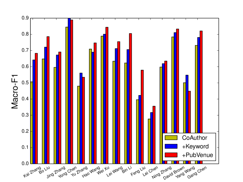
Figure 3: Feature contribution analysis using most recent 2 years’ publication records as test set

6.4 Study of Running Time

A very desirable feature of our proposed Bayesian non-exhaustive classification model is its running time. For example, using the most recent two years’ records as test set, on the name reference “Kai Zhang" containing $66$ papers with $10$ latent dimensionality, it takes around $0.29$ seconds on average to assign the test papers to different real-life authors for one-sweep Gibbs sampler. For the name reference “Lei Wang" with $308$ papers using same number of latent dimensionality, it takes around $1.95$ seconds on average under the same setting. This suggests only a linear increase in computational time with respect to the number of records. However in addition to number of records, the computational time depends on other factors, such as the latent dimensionality and the number of classes generated, which in turn depends on the values of the hyperparameters used in the data model.

7 Conclusion

To conclude, in this paper we propose a Bayesian non-exhaustive classification framework for online name entity disambiguation. Given sequentially observed record streams, our method classifies the incoming records into existing classes, as well as emerging classes by using one sweep Gibbs sampler for learning posterior probability of a Dirichlet process mixture model. Our experimental results on bibliographic datasets show that the proposed method significantly outperforms the existing state-of-the-arts for disambiguating authors’ name in online setting.

References

- [1] F. Akova, M. Dundar, V. J. Davisson, E. D. Hirleman, A. K. Bhunia, J. P. Robinson, and B. Rajwa. A machine-learning approach to detecting unknown bacterial serovars. Statistical Analysis and Data Mining, pages 289–301, 2010.
- [2] D. Aldous. Exchangeability and related topics. 1985.
- [3] T. W. Anderson, editor. An Introduction to Multivariate Statistical Analysis. 1984.
- [4] R. Bunescu and M. Pasca. Using encyclopedic knowledge for named entity disambiguation. In European Chapter of the Association for Comp. Linguistics, pages 9–16, 2006.
- [5] L. Cen, E. C. Dragut, L. Si, and M. Ouzzani. Author disambiguation by hierarchical agglomerative clustering with adaptive stopping criterion. In SIGIR, pages 741–744, 2013.
- [6] P.-Y. Chen, B. Zhang, M. A. Hasan, and A. O. Hero. Incremental method for spectral clustering of increasing orders. KDD Workshop on Mining and Learning with Graphs, 2016.
- [7] S. Choudhury, K. Agarwal, S. Purohit, B. Zhang, M. Pirrung, W. Smith, and M. Thomas. Nous: Construction and querying of dynamic knowledge graphs. arXiv preprint arXiv:1606.02314, 2016.
- [8] A. Davis, A. Veloso, A. S. da Silva, W. Meira, Jr., and A. H. F. Laender. Named entity disambiguation in streaming data. In ACL, 2012.
- [9] A. P. de Carvalho, A. A. Ferreira, A. H. F. Laender, and M. A. Goncalves. Incremental unsupervised name disambiguation in cleaned digital libraries. JIDM, pages 289–304, 2011.
- [10] M. Dundar, F. Akova, A. Qi, and B. Rajwa. Bayesian nonexhaustive learning for online discovery and modeling of emerging classes. In ICML, pages 113–120, 2012.
- [11] T. S. Ferguson. A bayesian analysis of some nonparametric problems. Ann. Statist., pages 209–230, 1973.
- [12] T. Greene and W. S.Rayens. Partially pooled covariance matrix estimation in discriminant analysis. Communications in Statistics - Theory and Methods, pages 3679–3702, 1989.
- [13] H. Han, L. Giles, H. Zha, C. Li, and K. Tsioutsiouliklis. Two supervised learning approaches for name disambiguation in author citations. In Joint Conf. on Digital Libraries, 2004.
- [14] H. Han, H. Zha, and C. L. Giles. Name disambiguation in author citations using a k-way spectral clustering method. In ACM Joint Conf. on Digital Libraries, pages 334–343, 2005.
- [15] L. Hermansson, T. Kerola, F. Johansson, V. Jethava, and D. Dubhashi. Entity disambiguation in anonymized graphs using graph kernels. In CIKM, pages 1037–1046, 2013.
- [16] J. Hoffart, Y. Altun, and G. Weikum. Discovering emerging entities with ambiguous names. In WWW, 2014.
- [17] M. Khabsa, P. Treeratpituk, and C. L. Giles. Online person name disambiguation with constraints. JCDL, 2015.
- [18] D. D. Lee and H. S. Seung. Algorithms for non-negative matrix factorization. In NIPS, pages 556–562. 2001.
- [19] D. Li and M. Becchi. Deploying graph algorithms on gpus: An adaptive solution. In IPDPS, 2013.
- [20] D. J. Michaud. Adventures in computer forensics. SANS Institute, 2001.
- [21] D. J. Miller and J. Browning. A mixture model and em-based algorithm for class discovery, robust classification, and outlier rejection in mixed labeled/unlabeled data sets. IEEE Transactions on PAMI, pages 1468–1483, 2003.
- [22] Y. Qian, Q. Zheng, T. Sakai, J. Ye, and J. Liu. Dynamic author name disambiguation for growing digital libraries. Journal of Inf. Retr., pages 379–412, 2015.
- [23] T. K. Saha, B. Zhang, and M. Al Hasan. Name disambiguation from link data in a collaboration graph using temporal and topological features. Social Network Analysis and Mining, pages 1–14, 2015.
- [24] G. Salton and M. J. McGill. Introduction to Modern Information Retrieval. 1986.
- [25] J. Sethuraman. A constructive definition of dirichlet priors. Statistica Sinica, pages 639–650, 1994.
- [26] Y. Song, J. Huang, I. G. Councill, J. Li, and C. L. Giles. Efficient topic-based unsupervised name disambiguation. In JCDL, pages 342–351, 2007.
- [27] J. Tang, A. C. M. Fong, B. Wang, and J. Zhang. A unified probabilistic framework for name disambiguation in digital library. IEEE TKDE, pages 975–987, 2012.
- [28] A. Veloso, A. A. Ferreira, M. A. Goncalves, A. H. F. Laender, and W. M. Jr. Cost-effective on-demand associative author name disambiguation. Inf. Process. Manage., 2012.
- [29] X. Wang, J. Tang, H. Cheng, and P. S. Yu. Adana: Active name disambiguation. In ICDM, pages 794–803, 2011.
- [30] B. Zhang, S. Choudhury, M. A. Hasan, X. Ning, K. Agarwal, S. Purohit, and P. G. P. Cabrera. Trust from the past: Bayesian personalized ranking based link prediction in knowledge graphs. SDM Workshop on Mining Networks and Graphs, 2016.
- [31] B. Zhang, N. Mohammed, V. Dave, and M. A. Hasan. Feature selection for classification under anonymity constraint. arXiv preprint arXiv:1512.07158, 2015.
- [32] B. Zhang, T. K. Saha, and M. A. Hasan. Name disambiguation from link data in a collaboration graph. In ASONAM, 2014.