Measurement of the CKM angle $\varphi_{1}$ in $B^{0}\to\overline{D}{}^{(*)0}h^{0}$, $\overline{D}{}^{0}\to K_{S}^{0}\pi^{+}\pi^{-}$ decays with time-dependent binned Dalitz plot analysis

Abstract

We report a measurement of the CP violation parameter $\varphi_{1}$ obtained in a time-dependent analysis of $B^{0}\to\overline{D}{}^{(*)0}h^{0}$ decays followed by $\overline{D}{}^{0}\to K_{S}^{0}\pi^{+}\pi^{-}$ decay. A model-independent measurement is performed using the binned Dalitz plot technique. The measured value is $\varphi_{1}=11.7^{\circ}\pm 7.8^{\circ}\left({\rm stat.}\right)\pm 2.1^{\circ}\left({\rm syst.}\right)$. Treating $\sin{2\varphi_{1}}$ and $\cos{2\varphi_{1}}$ as independent parameters, we obtain $\sin{2\varphi_{1}}=0.43\pm 0.27\left({\rm stat.}\right)\pm 0.08\left({\rm syst.}\right)$ and $\cos{2\varphi_{1}}=1.06\pm 0.33\left({\rm stat.}\right)^{+0.21}_{-0.15}\left({\rm syst.}\right)$. The results are obtained with a full data sample of $772\times 10^{6}B\overline{B}$ pairs collected near the $\Upsilon(4S)$ resonance with the Belle detector at the KEKB asymmetric-energy $e^{+}e^{-}$ collider.

I Introduction

The study of CP symmetry provides valuable insight into the structure and dynamics of matter from the subatomic to the cosmic scale. CP violation is a necessary ingredient for baryogenesis and explaining the state of matter in the observable Universe sakharov . The Standard Model (SM) of particle physics accounts for CP violation using the mechanism proposed by Kobayashi and Maskawa (KM) KM . A unitary matrix of quark flavor mixing, referred to as the Cabibbo-Kobayashi-Maskawa (CKM) cabibbo ; KM matrix, encodes this mechanism. The CKM matrix makes charged weak currents non-invariant under CP transformation. The SM does not predict the values of the elements of the CKM matrix, but theoretical predictions estimate that the amount of CP violation introduced by the SM is too feeble to explain the baryon asymmetry of the Universe baryogenesis . Thus, it is important to test the KM mechanism and search for new sources of CP violation.

(a)

(b)

Figure 1: $\overline{b}\to\overline{c}u\overline{d}$ transition (a) leading to $B^{0}\to\overline{D}{}^{0}h^{0}$ decay and $\overline{b}\to\overline{u}c\overline{d}$ transition (b) leading to $B^{0}\to D^{0}h^{0}$ decay.

Unitarity of the CKM matrix implies several relations among its elements that can be represented as triangles in the complex plane. In particular, the relation formed by the elements of the first and the third columns, referred to as the Unitarity Triangle (UT) ut , is the most accessible for experimental tests.

The CP violation parameter $\varphi_{1}=\arg(-\,V_{cd}V_{cb}^{*}/V_{td}V_{tb}^{*})$, where $V_{ij}$ is an element of the CKM matrix, is one of the angles of the UT. The value of $\sin{2\varphi_{1}}$ has been measured precisely in $b\to c\overline{c}s$ transitions by Belle, BaBar and LHCb sinbeta . Two discrete ambiguities remain with the known value of $\sin{2\varphi_{1}}$: $\varphi_{1}\to\varphi_{1}+\pi$ and $\varphi_{1}\to\pi/2-\varphi_{1}$. Currently, no theoretical approach is available to resolve the former ambiguity, but the latter can be resolved by measuring $\cos{2\varphi_{1}}$. Existing measurements of $\cos{2\varphi_{1}}$ in $b\to c\overline{u}d$ BaBarbdh0 ; belle_bdh0 and $b\to c\overline{c}s$ cosbeta_jphikst ; cosbeta_dstdstks transitions are much less precise and, in most cases, model-dependent.

Here, we present a model-independent measurement of the angle $\varphi_{1}$ in $b\to c\overline{u}d$ transitions (Fig. 1a) governing $B^{0}\to\overline{D}{}^{(*)0}h^{0}$ decays with subsequent $\overline{D}{}^{0}\to K_{S}^{0}\pi^{+}\pi^{-}$ decay, where $h^{0}$ is a light unflavored meson. This measurement is based on a data sample twice as large as that used in the previous $\varphi_{1}$ measurement using $B^{0}\to\overline{D}{}^{(*)0}h^{0}$ decays at Belle belle_bdh0 . The technique of a binned Dalitz plot analysis is applied to the $\varphi_{1}$ measurement for the first time.

I.1 Formalism

This section describes the technique to measure the angle $\varphi_{1}$ at an asymmetric-energy $e^{+}e^{-}$ collider operating at center-of-mass (${\rm CM}$) energy near the $\Upsilon(4S)$ resonance Sanda ; BPhys . When a pair of neutral $B$ mesons is produced, they oscillate coherently until one decays. Therefore, at the moment of a flavor-specific decay of one of the $B$ mesons (in the $\Upsilon(4S)$ rest frame), the flavor of the other $B$ meson is fixed. The former $B$ meson is referred to as the tagging $B$ meson and the latter as the signal $B$ meson. The tagging and signal $B$ mesons decay at proper times $t_{{\rm tag}}$ and $t_{{\rm sig}}$, respectively.

The longitudinal distance $\Delta z$ along the beam axis between the decay vertices of the signal and tagging $B$ mesons in the lab frame is measured. Since the $B$ mesons are produced almost at rest in the ${\rm CM}$ frame, their momentum can be neglected and the approximation $\Delta t\approx\Delta z/(c\beta\gamma)$ can be used, where $\Delta t=t_{{\rm sig}}-t_{{\rm tag}}$ and $\beta$ and $\gamma$ are the Lorentz factors of the $\Upsilon(4S)$ parent.

If the amplitudes $\mathcal{A}\left(B^{0}\to f\right)\equiv\mathcal{A}_{f}$ and $\mathcal{A}\left(\overline{B}{}^{0}\to f\right)\equiv\overline{\mathcal{A}}{}_{f}$ are non-zero for some final state $f$, then the distribution of the decay time difference, attributed to the interference of the processes $B^{0}\to~{}f$ and $B^{0}~{}\to~{}\overline{B}{}^{0}~{}\to~{}f$, is Sanda

$$\begin{split}\mathcal{P}(\Delta t)&=h_{1}e^{-\frac{\left|\Delta t\right|}{\tau_{B}}}\left[1+\frac{1-\left|\lambda_{f}\right|^{2}}{1+\left|\lambda_{f}\right|^{2}}\cos{\left(\Delta m_{B}\Delta t\right)}\right.\\ &\left.-\frac{2\,{\rm Im}\,\lambda_{f}}{1+\left|\lambda_{f}\right|^{2}}\sin{\left(\Delta m_{B}\Delta t\right)}\right],\quad\lambda_{f}=\frac{q}{p}\frac{\overline{\mathcal{A}}{}_{f}}{\mathcal{A}_{f}},\end{split}$$ (1)

where $p$ and $q$ are the coefficients relating the mass and flavor $B$-meson eigenstates to each other, $\tau_{B}$ is the neutral $B$ meson lifetime (assumed to be the same for both mass eigenstates), $\Delta m_{B}$ is the mass difference between the mass eigenstates, and $h_{1}$ is a normalizing constant. In the following, we assume the absence of CP violation in mixing and a null CP-violating weak phase in the $B$ meson decay amplitudes:

$$\frac{q}{p}=e^{-i2\varphi_{1}},\quad\arg\left(\frac{\overline{\mathcal{A}}{}_{f}}{\mathcal{A}_{f}}\right)=\Delta\delta_{f},$$ (2)

so that

$${\rm Im}\,\lambda_{f}=\left|\frac{\overline{\mathcal{A}}{}_{f}}{\mathcal{A}_{f}}\right|\sin{\left(\Delta\delta_{f}-2\varphi_{1}\right)};$$ (3)

here, $\Delta\delta_{f}$ is the difference in strong phases, which does not change sign under a CP transformation. Consideration of the CP-conjugated process, in which the CP-violating phase $\varphi_{1}$ is replaced by $-\varphi_{1}$, allows one to distinguish between the weak ($2\varphi_{1}$) and strong ($\Delta\delta_{f}$) phases.

For $B^{0}\to\overline{D}{}^{(*)0}h^{0}$ decays, the amplitudes $\mathcal{A}_{f}$ and $\overline{\mathcal{A}}{}_{f}$ can be expressed as

$$\mathcal{A}_{f}=\alpha_{B}\overline{\mathcal{A}}_{D},\quad\overline{\mathcal{A}}{}_{f}=\alpha_{B}\xi_{h^{0}}\left(-1\right)^{L}\mathcal{A}_{D},$$ (4)

where $\xi_{h^{0}}$ is the CP eigenvalue of the $h^{0}$ meson, $L$ is the relative angular momentum in the $D{}^{(*)0}h^{0}$ system, $\mathcal{A}_{D}$ ($\overline{\mathcal{A}}_{D}$) is the $D^{0}$ ($\overline{D}{}^{0}$) decay amplitude into the final state $f_{D}$, and $\alpha_{B}$ is a complex coefficient. The charm mixing and possible CP violation in the $D$ meson decays are neglected in Eq. (4). With the existing $B$-factories statistics, the $B^{0}\to D^{0}h^{0}$ decay amplitude (Fig. 1b) can be neglected with respect to the $B^{0}\to\overline{D}{}^{0}h^{0}$ decay amplitude (Fig. 1a) because it is suppressed by $\left|V_{ub}V_{cd}/V_{cb}V_{ud}\right|\approx 0.02$.

If the state $f_{D}$ is a CP eigenstate, then the entire state $f$ is CP eigenstate (except for the $\overline{D}{}^{*0}h^{0}$ state with a vector $h^{0}$ meson) as well and the phase $\Delta\delta_{f}$ equals $0$ or $\pi$. This exposes a sensitivity to $\sin{2\varphi_{1}}$ but not $\cos{2\varphi_{1}}$ and provides the best way to measure $\sin{2\varphi_{1}}$ in $b\to c\overline{u}d$ transitions markus_dcp .

The three-body state $f_{D}=K_{S}^{0}\pi^{+}\pi^{-}$ is not a CP eigenstate, so the phase $\Delta\delta_{f}$ is not limited to the values $0$ and $\pi$. As a consequence, this state provides sensitivity to both $\sin{2\varphi_{1}}$ and $\cos{2\varphi_{1}}$. The amplitude of $D^{0}\to K_{S}^{0}\pi^{+}\pi^{-}$ decay can be expressed as a function $\mathcal{A}_{D}$$\left(m_{+}^{2},m_{-}^{2}\right)$ of two Dalitz-distribution variables dalitz , where $m_{\pm}=m\left(K_{S}^{0}\pi^{\pm}\right)$ are the invariant masses. The amplitude $\overline{\mathcal{A}}_{D}$ of $\overline{D}{}^{0}\to K_{S}^{0}\pi^{+}\pi^{-}$ decay can be obtained by transposing the Dalitz variables: $\overline{\mathcal{A}}_{D}\left(m_{+}^{2},m_{-}^{2}\right)\equiv\mathcal{A}_{D}\left(m_{-}^{2},m_{+}^{2}\right)$. Therefore, the phase difference $\Delta\delta_{f}$ is a function of the Dalitz variables:

$$\begin{split}\Delta\delta_{f}\left(m_{+}^{2},m_{-}^{2}\right)&=\arg\left(\xi_{h^{0}}(-1)^{L}\right)-\Delta\delta_{D}\left(m_{+}^{2},m_{-}^{2}\right),\\ \Delta\delta_{D}\left(m_{+}^{2},m_{-}^{2}\right)&=\arg\left(\frac{\mathcal{A}_{D}\left(m_{-}^{2},m_{+}^{2}\right)}{\mathcal{A}_{D}\left(m_{+}^{2},m_{-}^{2}\right)}\right).\end{split}$$ (5)

For the $f_{D}=K_{S}^{0}\pi^{+}\pi^{-}$ final state, the strong phase $\Delta\delta_{D}$ cannot be measured at each point in the phase space: additional information is necessary. An approach based on an isobar model of the $D$ meson decay amplitude was proposed in Ref. BGK and used in the measurement of the CKM angle $\varphi_{1}$ performed by BaBar BaBarbdh0 and Belle belle_bdh0 . Alternatively, we use here a method that is independent of the decay model, as described below.

I.2 Time-dependent binned Dalitz plot analysis

Our measurement is based on the binned Dalitz distribution approach. This idea was proposed in Ref. GGSZ to measure the CKM angle $\varphi_{3}$ and further developed for several applications in Refs. BP_phi3_model ; BPV ; hr . We extend this approach to measure the angle $\varphi_{1}$ in the time-dependent analysis of $B^{0}\to\overline{D}{}^{(*)0}h^{0}$, $\overline{D}{}^{0}\to K_{S}^{0}\pi^{+}\pi^{-}$ decays. The Dalitz plot is divided into $16$ bins ($2\mathcal{N}$ in the general case) symmetrically with respect to $m_{+}^{2}\leftrightarrow m_{-}^{2}$ exchange. The bin index $i$ lies between $-8$ and $8$, excluding $0$; $m_{+}^{2}\leftrightarrow m_{-}^{2}$ exchange corresponds to the sign inversion $i\to-i$.

Several parameters related to a Dalitz plot bin on the Dalitz plane $\mathcal{D}$ are introduced. These are the probability for the $\overline{D}{}^{0}$ meson to decay into the phase space region $\mathcal{D}_{i}$ of the Dalitz plot bin $i$

$$K_{i}=\int\limits_{\mathcal{D}_{i}}\left|\mathcal{A}_{D}\left(m_{-}^{2},m_{+}^{2}\right)\right|^{2}dm_{+}^{2}dm_{-}^{2},$$ (6)

(normalized by $\sum_{i=-8}^{8}{K_{i}}=1$) and the weighted averages of the sine and cosine of the phase difference between $\overline{D}{}^{0}$ and $D^{0}$ decay amplitudes $\Delta\delta_{D}$ $\left(m_{+}^{2},m_{-}^{2}\right)$ over the $i$-th Dalitz plot bin:

$$\begin{split}&C_{i}=\frac{\int\limits_{\mathcal{D}_{i}}\left|\mathcal{A}_{D}\right|\left|\overline{\mathcal{A}}_{D}\right|\cos\Delta\delta_{D}\,dm_{+}^{2}dm_{-}^{2}}{\sqrt{K_{i}K_{-i}}},\\ &S_{i}=\frac{\int\limits_{\mathcal{D}_{i}}\left|\mathcal{A}_{D}\right|\left|\overline{\mathcal{A}}_{D}\right|\sin\Delta\delta_{D}\,dm_{+}^{2}dm_{-}^{2}}{\sqrt{K_{i}K_{-i}}}\,.\end{split}$$ (7)

The binning method yields the relations $C_{i}=C_{-i}$ and $S_{i}=-S_{-i}$. Eq. (1) can be expressed in the form appropriate for a time-dependent binned analysis:

$$\begin{split}\mathcal{P}_{i}\left(\Delta t,\varphi_{1}\right)&=h_{2}e^{-\frac{\left|\Delta t\right|}{\tau_{B}}}\left[1+q_{B}\frac{K_{i}-K_{-i}}{K_{i}+K_{-i}}\cos\left(\Delta m_{B}\Delta t\right)\right.\\ &\left.+2q_{B}\xi_{h^{0}}(-1)^{L}\frac{\sqrt{K_{i}K_{-i}}}{K_{i}+K_{-i}}\sin\left(\Delta m_{B}\Delta t\right)\left(S_{i}\cos{2\varphi_{1}}+C_{i}\sin{2\varphi_{1}}\right)\right],\end{split}$$ (8)

where $q_{B}=-1$ ($+1$) corresponds to a signal $B^{0}$ ($\overline{B}{}^{0}$) meson and $h_{2}$ is a normalizing constant.

The knowledge of the signal-event distribution over the Dalitz plot bins for both $B$ meson flavors is necessary for the fit that extracts the CP violation parameters. The expected fraction $n_{i,q_{B}}$ of signal events for the $i$-th Dalitz plot bin and signal $B$ flavor $q_{B}$ is

$$n_{i,q_{B}}=\frac{K_{i}+K_{-i}}{2}+\frac{q_{B}}{1+(\tau_{B}\Delta m_{B})^{2}}\cdot\frac{K_{i}-K_{-i}}{2}.$$ (9)

This formula is obtained by integrating Eq. (8) over $\Delta t$.

In principle, each pair $(i,-i)$ of bins provides enough information to measure the CP violation parameters if the values of parameters $K_{\pm i}$, $C_{i}$, and $S_{i}$ are known and do not equal zero.

(a)

(b)

Figure 2: Dalitz plot distribution (a) and equal-phase binning (b) obtained with the amplitude model of $\overline{D}{}^{0}\to K_{S}^{0}\pi^{+}\pi^{-}$ decay from Ref. Belle_model .

For a given binning of the Dalitz plot, the parameters $K_{i}$ can be measured with a set of flavor-tagged neutral $D$ mesons such as $D^{*+}\to D^{0}\pi^{+}$ or $B^{+}\to\overline{D}{}^{0}\pi^{+}$ decays, by measuring signal yield in each Dalitz plot bin. The measurement of the phase parameters $C_{i}$ and $S_{i}$ is more complicated and can be done with coherent decays of $D^{0}\overline{D}{}^{0}$ pairs CLEO_phasees .

Measurement of the CP violation parameters is possible for an arbitrary binning of the Dalitz plot, but usage of the realistic decay amplitude model allows one to optimize the binning to approach the maximal statistical sensitivity. In particular, the equal-phase binning method BP_phi3_model suggests the following rule for $i>0$ and $m_{+}^{2}<m_{-}^{2}$:

$$\frac{\pi(i-3/2)}{4}<\Delta\delta_{D}\left(m_{+}^{2},m_{-}^{2}\right)<\frac{\pi(i-1/2)}{4}.$$ (10)

This binning and the $D^{0}\to K_{S}^{0}\pi^{+}\pi^{-}$ decay amplitude model reported in Ref. Belle_model (see Fig. 2) are employed in the analysis presented here. The analysis uses the values of $K_{i}$ extracted from the $B^{+}\to\overline{D}{}^{0}\pi^{+}$ sample, as described in Section IV, and the values of $C_{i}$ and $S_{i}$ parameters measured by CLEO-c CLEO_phasees , as listed in Table 1.

Model-inspired binning of the Dalitz plot does not lead to a bias in the measured parameters, because of the excellent invariant mass resolution of the detector. Therefore, an alternative binning derived from a model that parameterized the data poorly would only reduce the statistical sensitivity of the measurement.

Table 1: The values of the parameters $C_{i}$ and $S_{i}$ measured by CLEO-c CLEO_phasees for equal-phase Dalitz-plot binning according to the $\overline{D}{}^{0}\to K_{S}^{0}\pi^{+}\pi^{-}$ decay model obtained in Ref. Belle_model .

Bin	$C_{i}$	$S_{i}$
$1$	$0.710\pm 0.034\pm 0.038$	$-0.013\pm 0.097\pm 0.031$
$2$	$0.481\pm 0.080\pm 0.070$	$-0.147\pm 0.177\pm 0.107$
$3$	$0.008\pm 0.080\pm 0.087$	$0.938\pm 0.120\pm 0.047$
$4$	$-0.757\pm 0.099\pm 0.065$	$0.386\pm 0.208\pm 0.067$
$5$	$-0.884\pm 0.056\pm 0.054$	$-0.162\pm 0.130\pm 0.041$
$6$	$-0.462\pm 0.100\pm 0.082$	$-0.616\pm 0.188\pm 0.052$
$7$	$0.106\pm 0.105\pm 0.100$	$-1.063\pm 0.174\pm 0.066$
$8$	$0.365\pm 0.071\pm 0.078$	$-0.179\pm 0.166\pm 0.048$

II Belle detector

This measurement is based on a data sample that contains $772\times 10^{6}~{}B\overline{B}$ pairs, collected with the Belle detector at the KEKB asymmetric-energy $e^{+}e^{-}$ ($3.5$ on $8$ GeV) collider KEKB operated near the $\Upsilon(4S)$ resonance.

The Belle detector is a large-solid-angle magnetic spectrometer that consists of a silicon vertex detector (SVD) featuring the double-sided silicon strip devices, a $50$-layer central drift chamber (CDC), an array of aerogel threshold Cherenkov counters, a barrel-like arrangement of time-of-flight scintillation counters, and an electromagnetic calorimeter comprised of CsI(Tl) crystals located inside a super-conducting solenoid coil that provides a $1.5$ T magnetic field. An iron flux-return located outside of the coil is instrumented to detect $K_{L}^{0}$ mesons and to identify muons. The detector is described in detail elsewhere Belle . Two inner detector configurations were used. A $2.0$ cm radius beampipe and a $3$-layer silicon vertex detector was used for the first sample of $152\times 10^{6}~{}B\overline{B}$ pairs, while a $1.5$ cm radius beampipe, a $4$-layer silicon vertex detector and a small-cell inner drift chamber were used to record the remaining $620\times 10^{6}~{}B\overline{B}$ pairs svd2 .

III Event selection

Six $B^{0}\to\overline{D}{}^{(*)0}h^{0}$ decay modes, $\overline{D}{}^{0}\pi^{0}$, $\overline{D}{}^{0}\eta$, $\overline{D}{}^{0}\eta^{\prime}$, $\overline{D}{}^{0}\omega$, $\overline{D}{}^{*0}\pi^{0}$, and $\overline{D}{}^{*0}\eta$, with subsequent decays $\overline{D}{}^{0}\to K_{S}^{0}\pi^{+}\pi^{-}$, $\eta\to\gamma\gamma$ or $\pi^{+}\pi^{-}\pi^{0}$, $\omega\to\pi^{+}\pi^{-}\pi^{0}$, $\eta^{\prime}\to[\gamma\gamma]_{\eta}\pi^{+}\pi^{-}$, and $\overline{D}{}^{*0}\to\overline{D}{}^{0}\pi^{0}$, are used in this analysis. Only $\eta\to\gamma\gamma$ is considered for the $\overline{D}{}^{0}\eta^{\prime}$ and $\overline{D}{}^{*0}\eta$ modes. Charged $B$-meson decay $B^{+}\to\overline{D}{}^{0}\pi^{+}$ followed by $\overline{D}{}^{0}\to K_{S}^{0}\pi^{+}\pi^{-}$ is used to measure the parameters $K_{i}$.

The charged pion candidates are selected from the reconstructed tracks and are required to have both $z$ and $r\varphi$ hits in at least one layer and at least one additional layer with a $z$ hit. The impact parameters of the tracks with respect to the beam interaction point in the longitudinal and transverse projections are required to satisfy $\left|dz\right|<5$ cm and $dr<2$ cm, respectively. The transverse momentum $p_{t}$ is required to be greater than $50~{}{\rm MeV/}c$ ($100~{}{\rm MeV/}c$) for pions produced in $D^{0}\to K_{S}^{0}\pi^{+}\pi^{-}$ ($h^{0}\to\pi^{+}\pi^{-}\pi^{0}$) decay. These requirements are not applied for the pions daughters of $K_{S}^{0}$ candidates.

The $K_{S}^{0}\to\pi^{+}\pi^{-}$ candidates are reconstructed from two oppositely charged tracks using two artificial neural networks (NN). The first NN is trained to suppress the combinatorial background and fake tracks: it uses the track impact parameters with respect to the beam interaction point, the azimuthal angle between the $K_{S}^{0}$ momentum and the decay-vertex vectors, the distance between the tracks, the $K_{S}^{0}$ flight length in the $x$-$y$ plane, the $K_{S}^{0}$ momentum, the distance between the beam interaction point and the tracks, the angle between the $K_{S}^{0}$ and a pion flight directions, the presence of the SVD hits and number of CDC hits on the tracks. The second NN is trained to suppress the background from $\Lambda\to p\pi^{-}$ decays: it uses the reconstructed mass with the lambda hypothesis, the absolute values of the track momenta, the track-momenta polar angles and the particle identification parameter distinguishing pions from protons. Further details of the procedure are described in Ref. nisks . The invariant mass of the selected candidates is required to be between $488.5$ and $506.5~{}{\rm MeV/}c^{2}$. This mass interval, as well as any other mass interval used in the analysis (unless explicitly stated otherwise), correspond to $\pm 3$ standard deviations from the nominal value.

The $\pi^{0}$ candidates are formed from photon pairs with an invariant mass between $115.7$ and $153.7~{}{\rm MeV/}c^{2}$. The photon energy is required to be greater than $40~{}{\rm MeV}$. The energy of the $\pi^{0}$ candidate from $h^{0}\to\pi^{+}\pi^{-}\pi^{0}$ ($h^{0}=\eta$ and $\omega$) decay must to be greater than $200~{}{\rm MeV}$.

The $\eta\to\gamma\gamma$ candidates are formed from photon pairs with an invariant mass between $530.0$ and $573.7~{}{\rm MeV/}c^{2}$. The photon energy is required to be greater than $80~{}{\rm MeV}$.

The $h^{0}\to\pi^{+}\pi^{-}\pi^{0}$ candidates, where $h^{0}~{}=~{}\eta$ or $\omega$, are formed from a $\pi^{0}$ candidate and two oppositely charged tracks with invariant mass between $537.6$ and $557.4~{}{\rm MeV/}c^{2}$ for $\eta$ and between $760.4$ and $803.9~{}{\rm MeV/}c^{2}$ for $\omega$. For the $\omega$ candidates, the absolute value of the cosine of the helicity angle $\theta_{\rm hel}$ (the angle between the $B^{0}$ flight direction and the normal to the $\omega$ decay plane in the $\omega$ rest frame) is required to be greater than $0.2$.

The $\eta^{\prime}\to\eta\pi^{+}\pi^{-}$ candidates are formed from a $\eta\to\gamma\gamma$ candidate and two oppositely charged tracks, both treated as pions. The invariant mass difference $\Delta m_{\eta}~{}\equiv~{}m(\eta^{\prime})-m(\eta)$ is required to lie between $401.7$ and $417.7~{}{\rm MeV/}c^{2}$.

The $D^{0}\to K_{S}^{0}\pi^{+}\pi^{-}$ candidates are formed from a $K_{S}^{0}$ candidate and two oppositely charged tracks, both treated as pions, with an invariant mass between $1.8516$ and $1.8783~{}{\rm GeV/}c^{2}$.

The $D^{*0}\to D^{0}\pi^{0}$ candidates are formed from a $D^{0}$ candidate and a neutral pion candidate. The invariant mass difference $\Delta m_{D}\equiv m(D^{*0})-m(D^{0})$ must lie between $140.2$ and $144.2~{}{\rm MeV/}c^{2}$.

The selection of $B^{0}$ and $B^{\pm}$ candidates is based on the variables $\Delta E~{}=~{}E^{{\rm CM}}_{B}-E^{{\rm CM}}_{{\rm beam}}$, the energy difference between the signal $B$ candidate and beam in the ${\rm CM}$ frame, and $M_{\rm bc}~{}=~{}\sqrt{\left(E^{{\rm CM}}_{{\rm beam}}/c^{2}\right)^{2}-\left(p^{{\rm CM}}_{B}/c\right)^{2}}$, the beam-energy constrained mass of the signal $B$ candidate. The candidates satisfying $|\Delta E|<0.3~{}{\rm GeV}$ and $M_{\rm bc}>5.2~{}{\rm GeV/}c^{2}$ are retained for further analysis.

The vertex-constrained kinematic fit is applied to the signal and tagging $B$ candidates and to the $D^{0}$ candidates. We require $\chi^{2}/{\rm n.d.f.}<500$ for the vertex-constrained fit of the $D^{0}$ meson candidates, where ${\rm n.d.f.}$ denotes the number of degrees of freedom.

When $h^{0}$ is a $\pi^{0}$ or $\eta\to\gamma\gamma$ candidate, the $B^{0}\to\overline{D}{}^{(*)0}h^{0}$ decay has no charged particle originating from the primary $B$ decay vertex. In this case, the $B$ decay vertex is determined by projecting the $D^{0}$-candidate trajectory onto the beam-interaction profile. The estimated longitudial resolution $\sigma_{z}$ of a such vertex, obtained from the fit, is required to be less than $0.5$ mm. This requirement is also imposed on the tagging $B$-decay vertices obtained by projecting a single track onto the beam interaction profile.

The vertex-constrained kinematic fit for other signal $B$ decay modes requires that the $D$ candidate trajectory and the two tracks from the $h^{0}$ decay originate from a common vertex and applies the Gaussian constraints on the position of this vertex based on the geometry of the beam interaction profile. The requirements $\sigma_{z}<0.2$ mm and $\chi^{2}/{\rm n.d.f.}<50$ for the vertex quality are imposed, where $\chi^{2}/{\rm n.d.f.}$ is calculated without taking into account the beam interaction profile constraint. These requirements are also imposed on the tagging $B$ decay vertices reconstructed with more than one track.

The vertex position for the tagging $B$ candidate is determined from the kinematic fit of well-reconstructed tracks that are not assigned to the signal $B$ candidate decay chain tagvtx .

The momentum of the $\pi^{0}$, $K_{S}^{0}$, and $\eta\to\gamma\gamma$ candidates, with the invariant mass constrained to its nominal value pdg , is used to improve the $\Delta E$ resolution. The momenta of the $D^{0}$ daughters obtained by a mass-constraint fit to the $D^{0}$ candidate are used to calculate the Dalitz variables.

The continuum background arising from $e^{+}e^{-}\to q\bar{q}$ (where $q=u,~{}d,~{}s,~{}c$) events is suppressed with the procedure described in Refs. SFW ; KSFW and with the BDT bdt1 ; bdt2 algorithm implemented within the TMVA tmva package.

The $b$ flavor of the tagging $B$ meson is identified from inclusive properties of particles that are not associated with the signal $B$ candidate TaggingNIM . The tagging information is represented by two parameters: the $b$-flavor charge $q$ and the purity $r$. The parameter $r$ is an event-by-event, MC-determined flavor-tagging dilution factor that ranges from $r=0$ for no flavor discrimination to $r=1$ for unambiguous flavor assignment. The data are sorted into seven intervals of $r$. For events with $r>0.1$, the wrong tag fractions for six $r$ intervals, $w_{l}$ ($l=1,2,\dots,6$), and their differences between $B^{0}$ and $\overline{B}{}^{0}$ decays, $\Delta w_{l}$, are determined from semileptonic and hadronic $b\to c$ decays Tagging . If $r\leq 0.1$, the wrong tag fraction is set to $0.5$ and the tagging information is not used. The total effective tagging efficiency, $\varepsilon_{\rm eff}=\sum(f_{l}\times(1-2w_{l})^{2})$, is $0.3$, where $f_{l}$ is the fraction of events in the category $l$. The parameter $Q_{B}=q_{B}\left(1-2w\right)/(1-q_{B}\Delta w)$ is used instead of the parameter $q_{B}$, defined in Eq. (8), to account for the wrong tag.

The signal yields of $B^{0}\to\overline{D}{}^{(*)0}h^{0}$ modes are obtained from an extended unbinned maximum likelihood fit of the $\Delta E$–$M_{\rm bc}$ two dimensional distribution in the region $\Delta E\,\in\,(-0.15~{}{\rm GeV},~{}0.30~{}{\rm GeV})\cap M_{\rm bc}\,\in\,(5.20~{}{\rm GeV/}c^{2},~{}5.29~{}{\rm GeV/}c^{2})$. The signal yield of $B^{+}\to\overline{D}{}^{0}\pi^{+}$ events is obtained from an extended unbinned maximum likelihood fit of the $\Delta E$ distribution in the region $(-0.10~{}{\rm GeV},~{}0.15~{}{\rm GeV})$ for $M_{\rm bc}~{}\in~{}(5.272~{}{\rm GeV/}c^{2},~{}5.287~{}{\rm GeV/}c^{2})$.

The sideband region is defined as the union of two rectangular regions in the $\Delta E$–$M_{\rm bc}$ plane: $M_{\rm bc}~{}\in~{}(5.23~{}{\rm GeV/}c^{2},~{}5.26~{}{\rm GeV/}c^{2})\ \cap\ \Delta E\ \in\ (-0.15~{}{\rm GeV},~{}0.30~{}{\rm GeV})$ and $M_{\rm bc}~{}\in~{}(5.26~{}{\rm GeV/}c^{2},~{}5.29~{}{\rm GeV/}c^{2})\ \cap\ \Delta E\ \in\ (0.12~{}{\rm GeV},~{}0.30~{}{\rm GeV})$.

The selection criteria and the analysis procedure are tested using the Monte Carlo (MC) simulation and fixed before performing the fit of the CP violation parameters. The MC events are generated with EvtGen evtgen . Final-state radiation from charged particles is simulated during the event generation using PHOTOS photos . The generated events are processed through the detailed detector simulation based on GEANT3 geant .

IV $B^{+}\to\overline{D}{}^{0}\pi^{+}$ sample

The $B^{+}\to\overline{D}{}^{0}\pi^{+}$ control sample is experimentally clean and has kinematic properties and detection efficiency similar to the $B^{0}\to\overline{D}{}^{(*)0}h^{0}$ decay. We use this process to select a sample of $D$ mesons in the flavor eigenstate and to measure the parameters $K_{i}$ defined in Eq. (6).

IV.1 Signal yield

Three components are included in the fit of the $\Delta E$ distribution: signal, $B^{+}\to\overline{D}{}^{0}K^{+}$ background and combinatorial background.

The signal distribution is parameterized by the sum of a Gaussian and two Crystal Ball functions CB with a common peak position. The mean and the Gaussian width are free fit parameters while the other parameters are fixed to the values obtained from simulation. Background from the $B^{+}\to\overline{D}{}^{0}K^{+}$ decays is parameterized by a Gaussian function with all parameters fixed from simulation. Combinatorial background is parameterized by a second-order Chebyshev polynomial. The parameters of the combinatorial background shape are obtained from the fit. The $\Delta E$ distribution for $B^{+}\to\overline{D}{}^{0}\pi^{+}$ candidates and the results of the fit are shown in Fig. 3. Yields of the signal and background components are listed in Table 2.

Figure 3: $\Delta E$ distribution for $B^{+}\to\overline{D}{}^{0}\pi^{+}$ candidates. Black circles with error bars show data, the solid blue line is the complete fit function, the dashed blue line is the signal component, the dashed black line is the background from $B^{+}\to\overline{D}{}^{0}K^{+}$ decays, the dashed brown line is the combinatorial background. Vertical red lines show the signal area. Histogram with the pulls of the data with respect to the fit curve is shown at the bottom (with horizontal blue dashed lines at pull values of $\pm 3$).

(a)

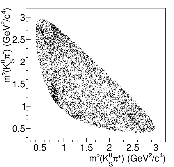
(b)

Figure 4: Dalitz plot distributions for $D\to K_{S}^{0}\pi^{+}\pi^{-}$ candidates with $D$ from $B^{+}\to\overline{D}{}^{0}\pi^{+}$ decay in the signal (a) and sideband (b) areas.

Table 2: Fit results of the $\Delta E$ distribution for $B^{+}\to\overline{D}{}^{0}\pi^{+}$ candidates. The numbers of events and the fraction of signal events are shown for the signal $\Delta E$ region.

Parameter	Value
Signal yield	$(1.375\pm 0.014)\times 10^{4}$
$B^{+}\to\overline{D}{}^{0}K^{+}$ yield	$18.7\pm 9.8$
Combinatorial bkg. yield	$1295\pm 79$
Signal fraction ($\%$)	$91.3\pm 0.9$

The parameters $K_{i}$ are measured using the events in the $\Delta E$ interval between $-30$ and $40~{}{\rm MeV}$. This interval is optimized to suppress the background from $B^{+}\to\overline{D}{}^{0}K^{+}$ events without significant signal-efficiency loss.

IV.2 Measurement of parameters $K_{i}$

The charged pion from the $B^{+}\to\overline{D}{}^{0}\pi^{+}$ decay tags the flavor of the $D$ meson. Therefore, the fraction of the signal events corresponding to the $i$-th Dalitz plot bin equals $K_{i}$.

The Dalitz distribution for $D\to K_{S}^{0}\pi^{+}\pi^{-}$ in the signal $\Delta E$ range, where the $D$ meson is produced in $B^{+}\to\overline{D}{}^{0}\pi^{+}$ decays, is shown in Fig. 4a. The fraction of signal, $f_{{\rm sig}}=(91.3\pm 0.9)\%$, is obtained from a fit of the $\Delta E$ distribution. The Dalitz plot for events from the $\Delta E$-$M_{\rm bc}$ sideband is shown in Fig. 4b. The binned background distribution is obtained from this data.

Table 3: The values of the parameters $K_{i}$ measured with the $B^{+}\to\overline{D}{}^{0}\pi^{+}$ data sample. The values are not corrected for the detection efficiency.

Bin ($i$)	$K_{i}$ (%)	$K_{-i}$ (%)
$1$	$17.42\pm 0.32$	$7.81\pm 0.25$
$2$	$7.51\pm 0.22$	$1.29\pm 0.10$
$3$	$10.24\pm 0.26$	$2.58\pm 0.14$
$4$	$2.85\pm 0.14$	$1.16\pm 0.10$
$5$	$9.45\pm 0.25$	$4.25\pm 0.17$
$6$	$7.31\pm 0.22$	$1.73\pm 0.11$
$7$	$10.48\pm 0.26$	$1.18\pm 0.10$
$8$	$12.46\pm 0.28$	$2.38\pm 0.14$

The values of the parameters $K_{i}$ are listed in Table 3. The uncertainties shown include the statistical uncertainty of the signal sample and the uncertainty due to background evaluation, added in quadrature. The systematic uncertainties associated with the background Dalitz plot distribution are neglected because the background fraction is very small.

V $B^{0}\to\overline{D}{}^{(*)0}h^{0}$ sample

V.1 Background components

Three background components are considered for the $B^{0}\to\overline{D}{}^{(*)0}h^{0}$ candidates:

• combinatorial background from non-resonant light quark production (continuum background);

• combinatorial background from $B\overline{B}$ events; and

• background from partially reconstructed $B$ decays.

Background from partially reconstructed decays is dominated by $B\to\overline{D}{}^{0}\rho$ and $B\to\overline{D}{}^{*}\pi^{0}$ for the $B^{0}\to\overline{D}{}^{0}\pi^{0}$ mode and by $B\to\overline{D}{}^{*}\rho$ for the $B^{0}\to\overline{D}{}^{*0}\pi^{0}$ mode. These processes, reconstructed with one missing pion, lead to a concentration below $-0.1~{}{\rm GeV}$ in the $\Delta E$ distribution. The background in all other channels is dominated by the combinatorial contribution with featureless $\Delta E$ distribution.

The background contribution from charmless $B^{0}$ decays is suppressed by requiring the presence of a $D^{0}$ candidate and thus is found to be negligible in this measurement.

V.2 Signal yield

A two-dimensional unbinned maximum likelihood fit of the $\Delta E$–$M_{\rm bc}$ distribution is performed for each signal mode. The probability density function (PDF) contains four components, corresponding to the signal and three backgrounds introduced above.

The signal $\Delta E$ distributions are parameterized by the sum of a Gaussian and two Crystal Ball functions with a common peak position. The signal $M_{\rm bc}$ distributions are parameterized by a function introduced in Ref. NskFcn and referred to as the Novosibirsk distribution. The peak position in the $\Delta E$–$M_{\rm bc}$ plane is obtained from the fit while the other parameters are fixed at the values obtained from simulation.

The $\Delta E$ distributions for events from continuum background are parameterized by a second-order Chebyshev polynomial. The $\Delta E$ distributions of the combinatorial background from the $B\overline{B}$ events are parameterized by an exponential function. The $M_{\rm bc}$ distributions of the combinatorial backgrounds are parameterized by an ARGUS function argus . The parameters of the $\Delta E$ PDF are obtained from the fit while those of the $M_{\rm bc}$ PDF are fixed at the values obtained from simulation.

(a)

(b)

(c)

(d)

Figure 5: $\Delta E$ fit projections for the signal $M_{\rm bc}$ regions (a, c) and $M_{\rm bc}$ fit projections for the signal $\Delta E$ regions (b, d) for the $B^{0}\to\overline{D}{}^{0}\pi^{0}$ (a, b) and $B^{0}\to\overline{D}{}^{0}\omega$ (c, d) candidates. Black circles with errors show data, continuous blue lines show projections of complete fit functions, dashed blue lines show signal components, dashed black lines show continuum background components, dashed brown lines show background from partially reconstructed $B$ decays and dot-dashed lines show combinatorial background from $B\overline{B}$ events. Histograms with the pulls of the data with respect to the fit curves are shown at the bottom of each plot (with horizontal blue dashed lines at pull values of $\pm 3$).

(a)

(b)

(c)

(d)

(e)

(f)

(g)

(h)

(i)

(j)

Figure 6: $\Delta E$ fit projections for the signal $M_{\rm bc}$ regions (a – e) and $M_{\rm bc}$ fit projections for the signal $\Delta E$ regions (f – j) for the $B^{0}\to\overline{D}{}^{0}\eta$, $\eta\to\gamma\gamma$ (a, f), $B^{0}\to\overline{D}{}^{0}\eta$, $\eta\to\pi^{+}\pi^{-}\pi^{0}$ (b, g), $B^{0}\to\overline{D}{}^{0}\eta^{\prime}$ (c, h), $B^{0}\to\overline{D}{}^{*0}\pi^{0}$ (d, i), and $B^{0}\to\overline{D}{}^{*0}\eta$ (e, j) candidates. Black circles with errors show data, continuous blue lines show projections of complete fit functions, dashed blue lines show signal components, dashed black lines show continuum background components, dashed brown lines show background from partially reconstructed $B$ decays and dot-dashed lines show combinatorial background from $B\overline{B}$ events.

The $\Delta E$ distributions of the background from partially reconstructed $B$ decays are parameterized by the following function:

$$\begin{split}p_{\rm pr}&(\Delta E)\propto 1+\zeta_{\rm l}\left(\Delta E-\Delta E_{0}\right)\\ &+s\ln\left(1+b\exp\left[{\frac{\left(\zeta_{\rm r}-\zeta_{\rm l}\right)\left(\Delta E-\Delta E_{0}\right)}{s}}\right]\right).\end{split}$$ (11)

This function describes two asymptotically straight lines smoothly merged near the point given by the $\Delta E_{0}$ parameter whose slopes are given by $\zeta_{\{{\rm r,l}\}}$. The parameter $s$ determines the curvature at the junction. If the $B$ candidate decay chain contains a $\pi^{0}$ or $\eta$ reconstructed in the $\gamma\gamma$ final state, the $M_{\rm bc}$ distribution of the background from partially reconstructed $B$ decays is parameterized by the Novosibirsk function; otherwise, it is parameterized by the sum of ARGUS and Gaussian functions. All parameters are fixed at the values obtained from simulation except for the values of the $\Delta E_{0}$ parameter for the $B^{0}\to\overline{D}{}^{0}\pi^{0}$ and $B^{0}\to\overline{D}{}^{*0}\pi^{0}$ modes that are obtained from the fit.

Several correlations between the $\Delta E$ and $M_{\rm bc}$ distributions are taken into account. A left-side tail of the signal $\Delta E$ distribution is due to $\pi^{0}$ or $\eta$ candidate where only one photon was identified correctly. This partially wrong combination leads to correlated shift both in $\Delta E$ and $M_{\rm bc}$. A similar correlation appears in the distributions of the background from partially reconstructed $B$ decays. The width of the signal $\Delta E$ distribution for the $B$ candidates with the $\eta$ or $\omega$ reconstructed in the $\pi^{+}\pi^{-}\pi^{0}$ final state is determined by the charged final state particles momentum resolution if both final state photons are correctly assigned. For such candidates, the $\Delta E$ and $M_{\rm bc}$ distributions are correlated. That correlation is accommodated by introducing a $\Delta E$ dependence of the signal $M_{\rm bc}$ PDF parameters. This parameterization is equivalent to a two-dimensional Gaussian function. No significant correlation is found for the combinatorial background. The values of parameters required to employ the correlations are obtained from simulation.

The fit projections for the $B^{0}\to\overline{D}{}^{0}\pi^{0}$ and $B^{0}\to\overline{D}{}^{0}\omega$ modes are shown in Fig. 5. The fit projections for the other signal modes are shown in Fig. 6. The fractions of background from partially reconstructed $B$ decays are small for all modes except $B^{0}\to\overline{D}{}^{0}\pi^{0}$ and $B^{0}\to\overline{D}{}^{*0}\pi^{0}$ (compare the $\Delta E$ distributions below $-0.1~{}{\rm GeV}$ for $B^{0}\to\overline{D}{}^{0}\pi^{0}$ and $B^{0}\to\overline{D}{}^{0}\omega$ in Fig. 5, for example) and cannot be determined from the fit. These fractions are fixed relative to the fractions of combinatorial background from $B\overline{B}$ events using the values obtained from MC simulation.

Table 4: Results of the $\Delta E$–$M_{\rm bc}$ fit for $B^{0}\to\overline{D}{}^{(*)0}h^{0}$ data. The numbers of events $N_{{\rm sig}}$ and the fractions $f_{{\rm sig}}$ of signal events obtained from the fit for the signal $\Delta E$–$M_{\rm bc}$ regions are shown.

Mode	$N_{{\rm sig}}$	$f_{{\rm sig}}$ (%)
$B^{0}\to\overline{D}{}^{0}\pi^{0}$	$464\pm 26$	$72.1\pm 4.1$
$B^{0}\to\overline{D}{}^{0}\eta_{\gamma\gamma}$	$99\pm 14$	$50.5\pm 7.0$
$B^{0}\to\overline{D}{}^{0}\eta_{\pi^{+}\pi^{-}\pi^{0}}$	$51.3\pm 8.8$	$66\pm 11$
$B^{0}\to\overline{D}{}^{0}\omega$	$182\pm 18$	$58.4\pm 5.7$
$B^{0}\to\overline{D}{}^{0}\eta^{\prime}$	$28.2\pm 6.4$	$70\pm 16$
$B^{0}\to\overline{D}{}^{*0}\pi^{0}$	$103\pm 17$	$44.1\pm 7.4$
$B^{0}\to\overline{D}{}^{*0}\eta$	$36.1\pm 7.6$	$64\pm 13$
Total	$962\pm 41$	$61\pm 2.6$

The ellipses in the $\Delta E$–$M_{\rm bc}$ plane inscribed in the rectangular areas marked by the vertical red lines in Figs. 5 and 6 are defined for each signal mode and are referred to as signal regions. The events in these signal regions are used in the fit of the CP violation parameters. The signal yields $N_{{\rm sig}}$ and fractions $f_{{\rm sig}}$ of signal events for each signal region obtained from the $\Delta E$–$M_{\rm bc}$ fit, are listed in Table 4. The Dalitz plots for events with a wrong-tag probability of under $23\%$ are shown in Fig. 7.

(a)

(b)

Figure 7: Dalitz distributions for $D$ mesons produced in tagged $B^{0}\to\overline{D}{}^{(*)0}h^{0}$ decays with wrong tag probability of less than $23\%$. The signal $B$ meson is tagged as $B^{0}$ (a) and $\overline{B}{}^{0}$ (b).

VI Determination of the CP violation parameters

(a)

(b)

Figure 8: Raw CP asymmetry distributions for the $B^{0}\to\overline{D}{}^{(*)0}h^{0}$ candidates in the $\pm 1$-st (a) and $\pm 5$-th (b) $D\to K_{S}^{0}\pi^{+}\pi^{-}$ decay Dalitz plot bins. Red lines are the result of the CP violation fit performed with the full data sample. The asymmetry for the $B^{0}\to\overline{D}{}^{*0}h^{0}$ candidates is taken with inverted sign.

(a)

(b)

Figure 9: $\Delta t$ distributions for the $B^{0}\to\overline{D}{}^{0}h^{0}$ candidates with wrong-tag probability of less than $23\%$. (a) ((b)) corresponds to the candidates from the $-3$-th ($7$-th) $D\to K_{S}^{0}\pi^{+}\pi^{-}$ Dalitz plot bin tagged as $B^{0}$ ($\overline{B}{}^{0}$). Continuous blue lines are the result of the CP violation fit performed with the full data sample. Dashed red lines are obtained with $\varphi_{1}=68.1^{\circ}$.

The CP violation parameters are measured using the unbinned maximum likelihood fit of the $\Delta t$ distribution. The likelihood function is defined as

$$\mathcal{L}=\prod\limits_{j=1}^{N}\left[(1-f_{{\rm bkg},j})p_{{\rm sig}}(\Delta t_{j})+f_{{\rm bkg},j}p_{{\rm bkg}}(\Delta t_{j})\right],$$ (12)

where the product is evaluated over all $N$ events in the sample, $f_{{\rm bkg},j}$ is the event-dependent background fraction obtained from the $\Delta E$–$M_{\rm bc}$ fit, $p_{{\rm sig}}$ is the signal PDF, and $p_{{\rm bkg}}$ is the background PDF.

The background $\Delta t$ distributions are parameterized by convolving the function

$$f_{\delta}\delta(\Delta t)+\left(1-f_{\delta}\right)2\tau_{{\rm bkg}}e^{-|\Delta t|/\tau_{{\rm bkg}}}$$ (13)

with a double-Gaussian function; here, $\delta$ is the Dirac delta function and $\tau_{{\rm bkg}}$ is the effective lifetime for background events. The widths of the double-Gaussian function are event-dependent and proportional to the estimated vertex resolution obtained from the vertex-constrained kinematic fits. The parameters $f_{\delta}$ and $\tau_{{\rm bkg}}$ are obtained from simulation while the parameters of the double-Gaussian function are obtained from the fit of the $\Delta t$ distribution in the $\Delta E$–$M_{\rm bc}$ sideband. The $\Delta t$ distributions for background from $B\overline{B}$ events and from continuum events are parameterized separately.

The signal $\Delta t$ distribution is parameterized by convolving Eq. (8) with a resolution function. The resolution function is described in Ref. vertexres . It is tuned for each event using information obtained from the vertex-constrained kinematic fits.

Table 5 shows results of the fit of the CP violation parameters, where $\sin{2\varphi_{1}}$ and $\cos{2\varphi_{1}}$ are treated as independent variables. The correlation coefficient of $\sin{2\varphi_{1}}$ and $\cos{2\varphi_{1}}$ is about $-3\%$.

Table 5: Fit of the CP violation parameters. Only statistical uncertainty is shown.

Signal mode	$\sin{2\varphi_{1}}$	$\cos{2\varphi_{1}}$
$B^{0}\to\overline{D}{}^{0}\pi^{0}$	$\phantom{-}0.61\pm 0.37$	$0.88^{+0.46}_{-0.52}$
$B^{0}\to\overline{D}{}^{0}\omega$	$-0.12\pm 0.58$	$1.28^{+0.62}_{-0.69}$
Other modes	$\phantom{-}0.44\pm 0.51$	$0.89^{+0.49}_{-0.55}$
All modes	$\phantom{-}0.41\pm 0.27$	$0.97\pm 0.33$

The combined fit of all signal modes, with the parameters $\sin{2\varphi_{1}}$ and $\cos{2\varphi_{1}}$ considered as functions of the angle $\varphi_{1}$, results in

$$\varphi_{1}=11.7^{\circ}\pm 7.8^{\circ}\left({\rm stat.}\right).$$ (14)

For illustration, the raw CP asymmetries for the Dalitz plot bins most sensitive to $\sin{2\varphi_{1}}$ are shown in Fig. 8. The $\Delta t$ distributions for the Dalitz plot bins most sensitive to $\cos{2\varphi_{1}}$ are shown in Fig. 9.

VII Systematic uncertainties

(a)

(b)

(c)

Figure 10: Negative double logarithm of profiled likelihood ratio Eq. (16) for $\sin{2\varphi_{1}}$ (a), $\cos{2\varphi_{1}}$ (b) and $\varphi_{1}$ (c) obtained with the Minos algorithm minos . Black squares mark $n\sigma$ standard confidence intervals corresponding to statistical uncertainty while blue circles mark $n\sigma$ standard confidence intervals corresponding to the overall uncertainty. Continuous blue and dashed black lines show $4$-th (a), (b) and $5$-th order (c) polynomial fit.

Table 6 provides the estimates of the systematic uncertainties in the measured values of the CP violation parameters.

The uncertainty due to the experimental resolution for the Dalitz variables is evaluated using the large sample of simulated signal events. The fit results are compared for the the CP violation fit performed using the reconstructed and the generated Dalitz-variables values. The uncertainty due to the detection-efficiency variation over the Dalitz plot is also evaluated using the simulated signal events. The fit results are compared for the CP violation fit performed with and without the efficiency correction.

The systematic uncertainty related to the signal $\Delta t$ parameterization is estimated by varying each resolution parameter by $\pm\sigma_{\pm}$ ($\pm 2\sigma_{\pm}$ for parameters obtained from MC simulation) and repeating the fit.

Other contributions to the systematic uncertainty (items $4$ – $10$ in Table 6) are evaluated simultaneously from the fit performed with nuisance parameters and the likelihood function expressed as follows:

$$-2\log{\mathcal{L}_{\rm n}}=-2\log{\mathcal{L}}+\sum\limits_{j,k}\left(p_{j}-p_{j}^{0}\right)\mathcal{K}_{jk}\left(p_{k}-p_{k}^{0}\right),$$ (15)

where $\mathcal{L}$ is defined in Eq. (12), $p_{j}$ and $p_{j}^{0}$ are the current and central values of the $j$-th nuisance parameter, respectively, $\mathcal{K}$ is the inverse covariance matrix for the nuisance parameters and the sum is evaluated over all nuisance parameters. The following nuisance parameters are introduced to evaluate the systematic uncertainty:

• the parameters $C_{i}$ and $S_{i}$ that give the dominant contribution (with the covariance matrix taken from the supplementary materials for Ref. CLEO_phasees ).

• the parameters $K_{i}$ with the uncertainties shown in Table 3;

• the yield of signal events in each Dalitz plot bin for each signal mode with the value and uncertainty obtained from the $\Delta E$–$M_{\rm bc}$ fit;

• the background $\Delta t$ PDF parameters with the values and uncertainties obtained from the fit of the $\Delta t$ distribution in the $\Delta E$–$M_{\rm bc}$ sideband;

• the parameters $\tau_{B}$ and $\Delta m_{B}$ with values and uncertainties taken from Ref. PDG ; and

• the average bias in the wrong-tag probability with the uncertainty obtained using the results from Ref. Tagging .

The flavor tagging procedure and the uncertainties in the $\Delta m_{B}$ and $\tau_{B}$ values give negligible contributions to the systematic uncertainty.

Frequentist confidence intervals for the CP violation parameters are evaluated using the profile likelihood method with likelihood ratios statistics

$$\lambda(\xi)=\frac{\mathcal{L}(\xi,\hat{\hat{p}})}{\mathcal{L}(\hat{\xi},\hat{p})},$$ (16)

where $\xi$ is $\sin{2\varphi_{1}}$ or $\cos{2\varphi_{1}}$ or $\varphi_{1}$, $\hat{\xi}$ is the optimal value, $\hat{p}$ represents the optimal values of all other parameters corresponding to $\hat{\xi}$, and $\hat{\hat{p}}$ represents the optimal values of all other parameters corresponding to the $\xi$ value. Negative double logarithms of the likelihood ratios are shown in Fig. 10.

Table 6: The sources and estimates of the systematic uncertainties for the CP violation parameters measured in the $B^{0}\to\overline{D}{}^{(*)0}h^{0}$ decays. The uncertainty $\sigma_{\rm nuis}$ due to the sources $4$ – $10$ is evaluated from the single fit varying all the nuisance parameters and using the likelihood function Eq. (15). The total systematic uncertainty $\sigma_{\rm syst}$ is calculated as $\sqrt{\sigma_{1}^{2}+\sigma_{2}^{2}+\sigma_{3}^{2}+\sigma_{\rm nuis}^{2}}$. The values related to the sources $4$ – $10$ are shown for illustration.

Source	$\delta_{\sin{2\varphi_{1}}}$ ($\%$)	$\delta_{\cos{2\varphi_{1}}}$ ($\%$)	$\delta_{\varphi_{1}}$ (deg)
1. Dalitz variables resol.	$0.3$	$0.7$	$0.1$
2. Detection efficiency	$0.6$	$0.8$	$0.2$
3. $\Delta t$ resolution	$3.8$	$6.7$	$1.2$
4. Flavor tagging	$0.1$	$0.1$	$<0.1$
5. $\Delta m_{B}$	$0.1$	$0.1$	$<0.1$
6. $\tau_{B}$	$0.1$	$0.1$	$<0.1$
7. $M_{\rm bc}$-$\Delta E$ fit	$3.4$	$1.9$	$0.8$
8. Bkg. $\Delta t$ param.	$3.6$	$3.1$	$0.7$
9. $K_{i}$	$3.2$	$2.0$	$0.7$
10. $C_{i}$ and $S_{i}$	$7.6$	${}^{+20}_{-13}$	$1.1$
$\sigma_{\rm nuis}$	$7.6$	${}^{+20}_{-13}$	$1.6$
Total $\sigma_{\rm syst}$	$8.5$	${}^{+21}_{-15}$	$2.1$
Stat. error for comparison	$\mathit{27}$	$\mathit{33}$	$\mathit{7.8}$

The dominant uncertainties shown in Table 6 could be reduced in high-statistics measurements at Belle II. Indeed, the uncertainties associated with the parameters $K_{i}$, the $\Delta t$ parameterization and the $\Delta E$–$M_{\rm bc}$ fit are determined by the size of the data sample. The parameters $C_{i}$ and $S_{i}$ can be measured more precisely with a large data set of coherently produced $D^{0}\overline{D}{}^{0}$ pairs collected by the BES - III experiment.

VIII Conclusions

A novel model-independent approach for measuring the CKM angle $\varphi_{1}$ has been developed and applied to the full data set of the Belle experiment. The following results are obtained:

$$\begin{split}\sin{2\varphi_{1}}&=0.43\pm 0.27\left({\rm stat.}\right)\pm 0.08\left({\rm syst.}\right),\\ \cos{2\varphi_{1}}&=1.06\pm 0.33\left({\rm stat.}\right)^{+0.21}_{-0.15}\left({\rm syst.}\right),\\ \varphi_{1}&=11.7^{\circ}\pm 7.8^{\circ}\left({\rm stat.}\right)\pm 2.1^{\circ}\left({\rm syst.}\right).\end{split}$$ (17)

The value $\sin{2\varphi_{1}}~{}=~{}0.691~{}\pm~{}0.017$ measured in $b\to c\overline{c}s$ transitions determines the absolute value of $\cos{2\varphi_{1}}$ leading to two possible solutions in the $0^{\circ}\leq\varphi_{1}<180^{\circ}$ range. Our measurement is inconsistent with the negative solution corresponding to the value $\varphi_{1}=68.1^{\circ}$ at the level of $5.1$ standard deviations but in agreement with the positive solution corresponding to the value $\varphi_{1}=21.9^{\circ}$ at $1.3$ standard deviations. Thus, this measurement clearly resolves the ambiguity in $\varphi_{1}$ inherent in the measurement of $\sin{2\varphi_{1}}$ using the $b\to c\overline{c}s$ transition.

This measurement supersedes the previous measurement of the $\sin{2\varphi_{1}}$ and $\cos{2\varphi_{1}}$ in $B^{0}\to\overline{D}{}^{(*)0}h^{0}$ decays at Belle belle_bdh0 . Nevertheless, it should be emphasized that a different analysis technique is used here. Furthermore, experimental information from $B^{+}\to\overline{D}{}^{0}\pi^{+}$ decays and from Ref. CLEO_phasees is used in this analysis but not in Ref. belle_bdh0 .

The binned Dalitz plot approach could be used for precise $\varphi_{1}$ measurements in $B^{0}\to\overline{D}{}^{(*)0}h^{0}$ followed by $\overline{D}{}^{0}\to K_{S}^{0}\pi^{+}\pi^{-}$ decays with the high-statistics data from the Belle II experiment. The dominant systematic uncertainties could be reduced with this larger data sample. Also, abundant coherently-produced $D^{0}\overline{D}{}^{0}$ pairs collected by the BES - III experiment can be used to improve our knowledge of the phase parameters $C_{i}$ and $S_{i}$. The number of Dalitz plot bins can be increased in future measurements to improve the statistical sensitivity to the CP violation parameters.

Some NP models predict the magnitude of CP violation to differ from the SM expectations acp_np . The difference may vary for different quark transitions. Thus, it would be interesting to compare the $\sin{2\varphi_{1}}$ value precisely measured in the $b\to c\overline{u}d$ transitions governing the $B^{0}\to\overline{D}{}^{(*)0}h^{0}$ decays with the $\sin{2\varphi_{1}}$ value precisely measured in the $b\to c\overline{c}s$ transitions.

IX Acknowledgments

We thank the KEKB group for the excellent operation of the accelerator; the KEK cryogenics group for the efficient operation of the solenoid; and the KEK computer group, the National Institute of Informatics, and the PNNL/EMSL computing group for valuable computing and SINET4 network support. We acknowledge support from the Ministry of Education, Culture, Sports, Science, and Technology (MEXT) of Japan, the Japan Society for the Promotion of Science (JSPS), and the Tau-Lepton Physics Research Center of Nagoya University; the Australian Research Council; Austrian Science Fund under Grant No. P 22742-N16 and P 26794-N20; the National Natural Science Foundation of China under Contracts No. 10575109, No. 10775142, No. 10875115, No. 11175187, No. 11475187 and No. 11575017; the Chinese Academy of Science Center for Excellence in Particle Physics; the Ministry of Education, Youth and Sports of the Czech Republic under Contract No. LG14034; the Carl Zeiss Foundation, the Deutsche Forschungsgemeinschaft, the Excellence Cluster Universe, and the VolkswagenStiftung; the Department of Science and Technology of India; the Istituto Nazionale di Fisica Nucleare of Italy; the WCU program of the Ministry of Education, National Research Foundation (NRF) of Korea Grants No. 2011-0029457, No. 2012-0008143, No. 2012R1A1A2008330, No. 2013R1A1A3007772, No. 2014R1A2A2A01005286, No. 2014R1A2A2A01002734, No. 2015R1A2A2A01003280 , No. 2015H1A2A1033649; the Basic Research Lab program under NRF Grant No. KRF-2011-0020333, Center for Korean J-PARC Users, No. NRF-2013K1A3A7A06056592; the Brain Korea 21-Plus program and Radiation Science Research Institute; the Polish Ministry of Science and Higher Education and the National Science Center; the Ministry of Education and Science of the Russian Federation and the Russian Foundation for Basic Research; the Slovenian Research Agency; Ikerbasque, Basque Foundation for Science and the Euskal Herriko Unibertsitatea (UPV/EHU) under program UFI 11/55 (Spain); the Swiss National Science Foundation; the Ministry of Education and the Ministry of Science and Technology of Taiwan; and the U.S. Department of Energy and the National Science Foundation. This work is supported by a Grant-in-Aid from MEXT for Science Research in a Priority Area (“New Development of Flavor Physics”) and from JSPS for Creative Scientific Research (“Evolution of Tau-lepton Physics”).

References

(1)
A. Sakharov, JETP 49, 345 (1965).
(2)
M. Kobayashi and T. Maskawa, Prog. Theor. Phys. 49, 652 (1973).
(5)
A.J. Buras and R. Fleischer, Adv. Ser. Direct. High Energy Phys. 15, 65 (1998).
(6)
The first measurements at -factories are published in
B. Aubert et al. (BaBar Collaboration), Phys. Rev. Lett. 87,
091801 (2001);
K. Abe et al. (Belle Collaboration), Phys. Rev. Lett. 87,
091802 (2001).
The most precise results at the moment are
B. Aubert et al. (BaBar Collaboration),
Phys. Rev. D 79, 072009 (2009);
I. Adachi et al. (Belle Collaboration),
Phys. Rev. Lett. 108, 171802 (2012);
R. Aaij et al. (LHCb collaboration),
Phys. Rev. Lett. 115, 031601 (2015).
(7)
B. Aubert et al. (BaBar Collaboration),
Phys. Rev. Lett. 99, 231802 (2007).
(8)
P. Krokovny et al. (Belle Collaboration),
Phys. Rev. Lett. 97, 081801 (2006).
(9)
R. Itoh et al. (Belle Collaboration),
Phys. Rev. Lett. 95, 091601 (2005);
B. Aubert et al. (The BaBar Collaboration),
Phys. Rev. D 71, 032005 (2005).
(10)
B. Aubert et al. (BaBar Collaboration),
Phys. Rev. D 74, 091101(R) (2006);
J. Dalseno et al. (Belle Collaboration),
Phys. Rev. D 76, 072004 (2007).
(11)
A. B. Carter and A. I. Sanda, Phys. Rev. Lett. 45, 952 (1980);
A. B. Carter and A. I. Sanda, Phys. Rev. D 23, 1567 (1981);
I. I. Bigi and A. I. Sanda, Nucl. Phys. 193, 85 (1981).
(12)
Ed. A.J. Bevan, B. Golob, Th. Mannel, S. Prell, and B.D. Yabsley,
Eur. Phys. J. C 74, (2014) 3026, SLAC-PUB-15968, KEK Preprint 2014-3.
(13)
A. Abdesselam et al. (BaBar Collaboration, Belle Collaboration)
Phys. Rev. Lett. 115, 121604 (2015).
(14)
R. H. Dalitz,
Phys. Rev. 94, 1046 (1954).
(15)
A. Bondar, T. Gershon, and P. Krokovny,
Phys. Lett. B 624, 1 (2005).
(16)
A. Giri, Y. Grossman, A. Soffer, and J. Zupan,
Phys. Rev. D 68, 054018 (2003).
(17)
A. Bondar and A. Poluektov,
Eur. Phys. J. C 47, 347 (2006); C 55, 51 (2008).
(18)
A. Bondar, A. Poluektov, and V. Vorobiev,
Phys. Rev. D 82, 034033 (2010).
(19)
S. Harnew and J. Rademacker, Phys. Lett. B 728, 296 (2014);
S. Harnew and J. Rademacker, JHEP 03, 169 (2015).
(20)
A. Poluektov et al. (Belle Collaboration),
Phys. Rev. D 81, 112002 (2010).
(21)
J. Libby et al. (CLEO Collaboration),
Phys. Rev. D 82, 112006 (2010).
(22)
S. Kurokawa and E. Kikutani,
Nucl. Instr. and. Meth. A 499, 1 (2003),
and other papers included in this volume.
(23)
A. Abashian et al. (Belle Collaboration),
Nucl. Instr. and Meth. A 479, 117 (2002).
(24)
Z. Natkaniec et al. (Belle SVD2 Group),
Nucl. Instrum. Meth. A 560, 1 (2006).
(25)
H. Nakano, Ph.D Thesis, Tohoku University (2014) Chapter 4, unpublished.
(26)
K. F. Chen et al. (Belle Collaboration), Phys. Rev. D 72, 012004 (2005).
(27)
K.A. Olive et al. (Particle Data Group),
Chin. Phys. C 38, 090001 (2014) and 2015 update.
(28)
The Fox-Wolfram moments were introduced in
G. C. Fox and S. Wolfram, Phys. Rev. Lett. 41, 1581 (1978).
The Fisher discriminant used by Belle, based on modified Fox-Wolfram moments (SFW), is described in
K. Abe et al. (Belle Collaboration), Phys. Rev. Lett. 87, 101801 (2001) and
K. Abe et al. (Belle Collaboration), Phys. Lett. B 511, 151 (2001).
(29)
S. H. Lee et al. (Belle Collaboration),
Phys. Rev. Lett. 91, 261801 (2003).
(30)
L. Breiman, J.H. Friedman, R.A. Olshen and C.J. Stone, Classification and
regression trees, Wadsworth international group, Belmont, California, USA, 1984.
(31)
R.E. Schapire and Y. Freund,
Jour. Comp. and Syst. Sc. 55, 119 (1997).
(32)
A. Hoecker et al., TMVA: Toolkit for multivariate data analysis, PoS ACAT 040 (2007), arXiv:physics/0703039.
(33)
H. Kakuno et al.,
Nucl. Instr. and Meth. A 533, 516 (2004).
(34)
K. Abe et al. (Belle Collaboration), Phys. Rev. D 71, 072003 (2005);
K.F. Chen et al. (Belle Collaboration), Phys. Rev. D 72, 012004 (2005);
H. Sahoo et al. (Belle Collaboration), Phys. Rev. D 77, 091103 (2008).