Cantor Meets Scott: Semantic
Foundations for Probabilistic Networks

Abstract

ProbNetKAT is a probabilistic extension of NetKAT with a denotational semantics based on Markov kernels. The language is expressive enough to generate continuous distributions, which raises the question of how to compute effectively in the language. This paper gives an new characterization of ProbNetKAT’s semantics using domain theory, which provides the foundation needed to build a practical implementation. We show how to use the semantics to approximate the behavior of arbitrary ProbNetKAT programs using distributions with finite support. We develop a prototype implementation and show how to use it to solve a variety of problems including characterizing the expected congestion induced by different routing schemes and reasoning probabilistically about reachability in a network.

1 Introduction

The recent emergence of software-defined networking (SDN) has led to the development of a number of domain-specific programming languages Foster et al. [2011]; Monsanto et al. [2013]; Voellmy et al. [2013]; Nelson et al. [2014] and reasoning tools Kazemian et al. [2012]; Khurshid et al. [2013]; Anderson et al. [2014]; Foster et al. [2015] for networks. But there is still a large gap between the models provided by these languages and the realities of modern networks. In particular, most existing SDN languages have semantics based on deterministic packet-processing functions, which makes it impossible to encode probabilistic behaviors. This is unfortunate because in the real world, network operators often use randomized protocols and probabilistic reasoning to achieve good performance.

Previous work on ProbNetKAT Foster et al. [2016] proposed an extension to the NetKAT language Anderson et al. [2014]; Foster et al. [2015] with a random choice operator that can be used to express a variety of probabilistic behaviors. ProbNetKAT has a compositional semantics based on Markov kernels that conservatively extends the deterministic NetKAT semantics and has been used to reason about various aspects of network performance including congestion, fault tolerance, and latency. However, although the language enjoys a number of attractive theoretical properties, there are some major impediments to building a practical implementation: (i) the semantics of iteration is formulated as an infinite process rather than a fixpoint in a suitable order, and (ii) some programs generate continuous distributions. These factors make it difficult to determine when a computation has converged to its final value, and there are also challenges related to representing and analyzing distributions with infinite support.

This paper introduces a new semantics for ProbNetKAT, following the approach pioneered by Saheb-Djahromi, Jones, and Plotkin Saheb-Djahromi [1980, 1978]; Jones [1989]; Plotkin [1982]; Jones and Plotkin [1989]. Whereas the original semantics of ProbNetKAT was somewhat imperative in nature, being based on stochastic processes, the semantics introduced in this paper is purely functional. Nevertheless, the two semantics are closely related—we give a precise, technical characterization of the relationship between them. The new semantics provides a suitable foundation for building a practical implementation, it provides new insights into the nature of probabilistic behavior in networks, and it opens up several interesting theoretical questions for future work.

Our new semantics follows the order-theoretic tradition established in previous work on Scott-style domain theory Scott [1972]; Abramsky and Jung [1994]. In particular, Scott-continuous maps on algebraic and continuous DCPOs both play a key role in our development. However, there is an interesting twist: NetKAT and ProbNetKAT are not state-based as with most other probabilistic systems, but are rather throughput-based. A ProbNetKAT program can be thought of as a filter that takes an input set of packet histories and generates an output randomly distributed on the measurable space $\smash{2^{\mathsf{H}}}$ of sets of packet histories. The closest thing to a “state” is a set of packet histories, and the structure of these sets (e.g., the lengths of the histories they contain and the standard subset relation) are important considerations. Hence, the fundamental domains are not flat domains as in traditional domain theory, but are instead the DCPO of sets of packet histories ordered by the subset relation. Another point of departure from prior work is that the structures used in the semantics are not subprobability distributions, but genuine probability distributions: with probability $1$, some set of packets is output, although it may be the empty set.

It is not obvious that such an order-theoretic semantics should exist at all. Traditional probability theory does not take order and compositionality as fundamental structuring principles, but prefers to work in monolithic sample spaces with strong topological properties such as Polish spaces. Prototypical examples of such spaces are the real line, Cantor space, and Baire space. The space of sets of packet histories $\smash{2^{\mathsf{H}}}$ is homeomorphic to the Cantor space, and this was the guiding principle in the development of the original ProbNetKAT semantics. Although the Cantor topology enjoys a number of attractive properties (compactness, metrizability, strong separation) that are lost when shifting to the Scott topology, the sacrifice is compensated by a more compelling least-fixpoint characterization of iteration that aligns better with the traditional domain-theoretic treatment. Intuitively, the key insight that underpins our development is the observation that ProbNetKAT programs are monotone: if a larger set of packet histories is provided as input, then the likelihood of seeing any particular set of packets as a subset of the output set can only increase. From this germ of an idea, we formulate an order-theoretic semantics for ProbNetKAT.

In addition to the strong theoretical motivation for this work, our new semantics also provides a source of practical useful reasoning techniques, notably in the treatment of iteration and approximation. The original paper on ProbNetKAT showed that the Kleene star operator satisfies the usual fixpoint equation $P^{*}=1\mathbin{\&}P\mathbin{;}P^{*}$, and that its finite approximants $P^{(n)}$ converge weakly (but not pointwise) to it. However, it was not characterized as a least fixpoint in any order or as a canonical solution in any sense. This was a bit unsettling and raised questions as to whether it was the “right” definition—questions for which there was no obvious answer. This paper characterizes $P^{*}$ as the least fixpoint of the Scott-continuous map $X\mapsto 1\mathbin{\&}P\mathbin{;}X$ on a continuous DCPO of Scott-continuous Markov kernels. This not only corroborates the original definition as the “right” one, but provides a powerful tool for monotone approximation. Indeed, this result implies the correctness of our prototype implementation, which we have used to build and evaluate several applications inspired by common real-world scenarios.

Contributions.

This main contributions of this paper are as follows: (i) we develop a domain-theoretic foundation for probabilistic network programming, (ii) using this semantics, we build a prototype implementation of the ProbNetKAT language, and (iii) we evaluate the applicability of the language on several case studies.

Outline.

The paper is structured as follows. In §2 we give a high-level overview of our technical development using a simple running example. In §3 we review basic definitions from domain theory and measure theory. In §4 we formalize the syntax and semantics of ProbNetKAT abstractly in terms of a monad. In §5 we prove a general theorem relating the Scott and Cantor topologies on $\smash{2^{\mathsf{H}}}$. Although the Scott topology is much weaker, the two topologies generate the same Borel sets, so the probability measures are the same in both. We also show that the bases of the two topologies are related by a countably infinite-dimensional triangular linear system, which can be viewed as an infinite analog of the inclusion-exclusion principle. The cornerstone of this result is an extension theorem (Theorem 8) that determines when a function on the basic Scott-open sets extends to a measure. In §6 we give the new domain-theoretic semantics for ProbNetKAT in which programs are characterized as Markov kernels that are Scott-continuous in their first argument. We show that this class of kernels forms a continuous DCPO, the basis elements being those kernels that drop all but fixed finite sets of input and output packets. In §7 we show that ProbNetKAT’s primitives are (Scott-)continuous and its program operators preserve continuity. Other operations such as product and Lebesgue integration are also treated in this framework. In proving these results, we attempt to reuse general results from domain theory whenever possible, relying on the specific properties of $\smash{2^{\mathsf{H}}}$ only when necessary. We supply complete proofs for folklore results and in cases where we could not find an appropriate original source. We also show that the two definitions of the Kleene star operator—one in terms of an infinite stochastic process and one as the least fixpoint of a Scott-continuous map—coincide. In §8 we apply the continuity results from §7 to derive monotone convergence theorems. In §9 we describe a prototype implementation based on §8 and several applications. In §10 we review related work. We conclude in §11 by discussing open problems and future directions.

2 Overview

This section provides motivation for the ProbNetKAT language and summarizes our main results using a simple example.

Example.

Consider the topology shown in Figure 1 and suppose we are asked to implement a routing application that forwards all traffic to its destination while minimizing congestion, gracefully adapting to shifts in load, and also handling unexpected failures. This problem is known as traffic engineering in the networking literature and has been extensively studied Fortz et al. [2002]; He and Rexford [2008]; Jain et al. [2013]; Applegate and Cohen [2003]; Räcke [2008]. Note that standard shortest-path routing (SPF) does not solve the problem as stated—in general, it can lead to bottlenecks and also makes the network vulnerable to failures. For example, consider sending a large amount of traffic from host $h_{1}$ to host $h_{3}$: there are two paths in the topology, one via switch $S_{2}$ and one via switch $S_{4}$, but if we only use a single path we sacrifice half of the available capacity. The most widely-deployed approaches to traffic engineering today are based on using multiple paths and randomization. For example, Equal Cost Multipath Routing (ECMP), which is widely supported on commodity routers, selects a least-cost path for each traffic flow uniformly at random. The intention is to spread the offered load across a large set of paths, thereby reducing congestion without increasing latency.

ProbNetKAT Language.

Using ProbNetKAT, it is straightforward to write a program that captures the essential behavior of ECMP. We first construct programs that model the routing tables and topology, and build a program that models the behavior of the entire network.

Routing: We model the routing tables for the switches using simple ProbNetKAT programs that match on destination addresses and forward packets on the next hop toward their destination. To randomly map packets to least-cost paths, we use the choice operator ($\oplus$). For example, the program for switch S1 in Figure 1 is as follows:

$$\begin{array}[]{@{~}r@{\,}l@{~}}{}\lx@intercol\hfil p_{1}&\mathrel{\smash{\triangleq}}(\mathsf{dst}\kern 0.43057pt{=}\kern 0.43057pth_{1}\mathbin{;}\mathsf{pt}\kern 0.43057pt{\leftarrow}\kern 0.43057pt1)\hfil~{}\\ {}\lx@intercol\hfil&\mathbin{\&}~{}(\mathsf{dst}\kern 0.43057pt{=}\kern 0.43057pth_{2}\mathbin{;}\mathsf{pt}\kern 0.43057pt{\leftarrow}\kern 0.43057pt2)\hfil~{}\\ {}\lx@intercol\hfil&\mathbin{\&}~{}(\mathsf{dst}\kern 0.43057pt{=}\kern 0.43057pth_{3}\mathbin{;}(\mathsf{pt}\kern 0.43057pt{\leftarrow}\kern 0.43057pt2\oplus\mathsf{pt}\kern 0.43057pt{\leftarrow}\kern 0.43057pt4))\hfil~{}\\ {}\lx@intercol\hfil&\mathbin{\&}~{}(\mathsf{dst}\kern 0.43057pt{=}\kern 0.43057pth_{4}\mathbin{;}\mathsf{pt}\kern 0.43057pt{\leftarrow}\kern 0.43057pt4)\hfil~{}\end{array}$$

The programs for other switches are similar. To a first approximation, this program can be read as a routing table, whose entries are separated by the parallel composition operator ($\mathbin{\&}$). The first entry states that packets whose destination is $h_{1}$ should be forwarded out on port $1$ (which is directly connected to $h_{1}$). Likewise, the second entry states that packets whose destination is host $h_{2}$ should be forwarded out on port $2$, which is the next hop on the unique shortest path to $h_{2}$. The third entry, however, is different: it states that packets whose destination is $h_{3}$ should be forwarded out on ports $2$ and $4$ with equal probability. This divides traffic going to $h_{3}$ among the clockwise path via $S_{2}$ and the counter-clockwise path via $S_{4}$. The final entry states that packets whose destination is $h_{4}$ should be forwarded out on port $4$, which is again the next hop on the unique shortest path to $h_{4}$. The routing program for the network is the parallel composition of the programs for each switch:

$$p\mathrel{\smash{\triangleq}}(\mathsf{sw}\kern 0.43057pt{=}\kern 0.43057ptS_{1}\mathbin{;}p_{1})\mathbin{\&}(\mathsf{sw}\kern 0.43057pt{=}\kern 0.43057ptS_{2}\mathbin{;}p_{2})\mathbin{\&}(\mathsf{sw}\kern 0.43057pt{=}\kern 0.43057ptS_{3}\mathbin{;}p_{3})\mathbin{\&}(\mathsf{sw}\kern 0.43057pt{=}\kern 0.43057ptS_{4}\mathbin{;}p_{4})$$

Topology: We model a directed link as a program that matches on the switch and port at one end of the link and modifies the switch and port to the other end of the link. We model an undirected link $l$ as a parallel composition of directed links in each direction. For example, the link between switches $S_{1}$ and $S_{2}$ is modeled as follows:

$$l_{1,2} \triangleq({\mathsf{sw}\kern 0.43057pt{=}\kern 0.43057ptS_{1}\mathbin{;}\mathsf{pt}\kern 0.43057pt{=}\kern 0.43057pt2\mathbin{;}\mathsf{dup}}\mathbin{;}\mathsf{sw}\kern 0.43057pt{\leftarrow}\kern 0.43057ptS_{2}\mathbin{;}\mathsf{pt}\kern 0.43057pt{\leftarrow}\kern 0.43057pt1\mathbin{;}\mathsf{dup})$$

$$\mathbin{\&}({\mathsf{sw}\kern 0.43057pt{=}\kern 0.43057ptS_{2}\mathbin{;}\mathsf{pt}\kern 0.43057pt{=}\kern 0.43057pt1\mathbin{;}\mathsf{dup}}\mathbin{;}\mathsf{sw}\kern 0.43057pt{\leftarrow}\kern 0.43057ptS_{1}\mathbin{;}\mathsf{pt}\kern 0.43057pt{\leftarrow}\kern 0.43057pt2\mathbin{;}\mathsf{dup})$$

Note that at each hop we use ProbNetKAT’s $\mathsf{dup}$ operator to store the headers in the packet’s history, which records the trajectory of the packet as it goes through the network. Histories are useful for tasks such as measuring path length and analyzing link congestion. We model the topology as a parallel composition of individual links:

$$t~{}\triangleq~{}l_{1,2}~{}\mathbin{\&}~{}l_{2,3}~{}\mathbin{\&}~{}l_{3,4}~{}\mathbin{\&}~{}l_{1,4}$$

To delimit the network edge, we define ingress and egress predicates:

$$\begin{array}[]{rcl}\mathit{in}&\mathrel{\smash{\triangleq}}&(\mathsf{sw}\kern 0.43057pt{=}\kern 0.43057pt1\mathbin{;}\mathsf{pt}\kern 0.43057pt{=}\kern 0.43057pt1)\mathbin{\&}(\mathsf{sw}\kern 0.43057pt{=}\kern 0.43057pt2\mathbin{;}\mathsf{pt}\kern 0.43057pt{=}\kern 0.43057pt2)\mathbin{\&}\dots\\ \mathit{out}&\mathrel{\smash{\triangleq}}&(\mathsf{sw}\kern 0.43057pt{=}\kern 0.43057pt1\mathbin{;}\mathsf{pt}\kern 0.43057pt{=}\kern 0.43057pt1)\mathbin{\&}(\mathsf{sw}\kern 0.43057pt{=}\kern 0.43057pt2\mathbin{;}\mathsf{pt}\kern 0.43057pt{=}\kern 0.43057pt2)\mathbin{\&}\dots\\ \end{array}$$

Here, since every ingress is an egress, the predicates are identical.

Network: We model the end-to-end behavior of the entire network by combining $p$, $t$, $\mathit{in}$ and $\mathit{out}$ into a single program:

$$\mathit{net}\mathrel{\smash{\triangleq}}\mathit{in}\mathbin{;}(p\mathbin{;}t)^{*}\mathbin{;}p\mathbin{;}\mathit{out}$$

This program models processing each input from ingress to egress across a series of switches and links. Formally it denotes a Markov kernel that, when supplied with an input distribution on packet histories $\mu$ produces an output distribution $\nu$.

Queries: Having constructed a probabilistic model of the network, we can use standard tools from measure theory to reason about performance. For example, to compute the expected congestion on a given link $l$, we would introduce a function $Q$ from sets of packets to $\mathbb{R}\cup\{\infty\}$ (formally a random variable):

$$Q(a)\mathrel{\smash{\triangleq}}\sum_{h\in a}~{}\#_{l}(h)$$

where $\#_{l}(h)$ is the function on packet histories that returns the number of times that link $l$ occurs in $h$, and then compute the expected value of $Q$ using integration:

$$\operatorname*{\mathbf{E}}_{\nu}[Q]=\int Q\,d\nu$$

We can compute queries that capture other aspects of network performance such as latency, reliability, etc. in similar fashion.

Limitations.

Unfortunately there are several issues with the approach just described:

• One problem is that computing the results of a query can require complicated measure theory since a ProbNetKAT program may generate a continuous distribution in general (Lemma 4). Formally, instead of summing over the support of the distribution, we have to use Lebesgue integration in an appropriate measurable space. Of course, there are also challenges in representing infinite distributions in an implementation.

• Another issue is that the semantics of iteration is modeled in terms of an infinite stochastic process rather than a standard fixpoint. The original ProbNetKAT paper showed that it is possible to approximate a program using a series of star-free programs that weakly converge to the correct result, but the approximations need not converge monotonically, which makes this result difficult to apply in practice.

• Even worse, many of the queries that we would like to answer are not actually continuous in the Cantor topology, meaning that the weak convergence result does not even apply! The notion of distance on sets of packet histories is $d(a,b)=2^{-n}$ where $n$ is the length of the smallest history in $a$ but not in $b$, or vice versa. It is easy to construct a sequence of histories $h_{n}$ of length $n$ such that $\lim_{n\to\infty}d(\{h_{n}\},\{\})=0$ but $\lim_{n\to\infty}Q(\{h_{n}\})=\infty$ which is not equal to $Q(\{\})=0$.

Together, these issues are significant impediments that make it difficult to apply ProbNetKAT in many scenarios.

(a)

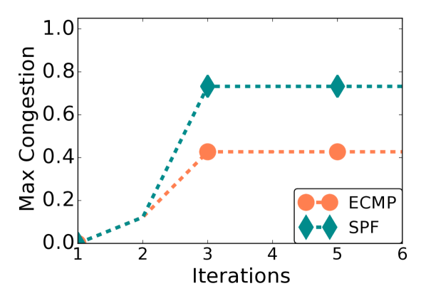
   (b)

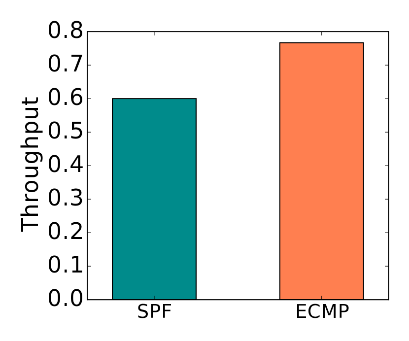
  (c)

Figure 1: (a) topology, (b) congestion, (c) failure throughput.

Domain-Theoretic Semantics.

This paper develops a new semantics for ProbNetKAT that overcomes these problems and provides the key building blocks needed to engineer a practical implementation. The main insight is that we can formulate the semantics in terms of the Scott topology rather than the Cantor topology. It turns out that these two topologies generate the same Borel sets, and the relationship between them can be characterized using an extension theorem that captures when functions on the basic Scott-open sets extend to a measure. We show how to construct a DCPO equipped with a natural partial order that also lifts to a partial order on Markov kernels. We prove that standard program operators are continuous, which allows us to formulate the semantics of the language—in particular Kleene star—using standard tools from domain theory, such as least fixpoints. Finally, we formalize a notion of approximation and prove a monotone convergence theorem.

The problems with the original ProbNetKAT semantics identified above are all solved using the new semantics. Because the new semantics models iteration as a least fixpoint, we can work with finite distributions and star-free approximations that are guaranteed to monotonically converge to the analytical solution (Corollary 23). Moreover, whereas our query $Q$ was not Cantor continuous, it is straightforward to show that it is Scott continuous. Let $A$ be an increasing chain $a_{0}\subseteq a_{1}\subseteq a_{2}\subseteq\dots$ ordered by inclusion. Scott continuity requires $\bigsqcup_{a\in A}Q(a)=Q(\bigsqcup A\big{)}$ which is easy to prove. Hence, the convergence theorem applies and we can compute a monotonically increasing chain of approximations that converge to $\operatorname*{\mathbf{E}}_{\nu}[Q]$.

Implementation and Applications.

We developed the first implementation of ProbNetKAT using the new semantics. We built an interpreter for the language and implemented a variety of traffic engineering schemes including ECMP, $k$-shortest path routing, and oblivious routing Räcke [2008]. We analyzed the performance of each scheme in terms of congestion and latency on real-world demands drawn from Internet2’s Abilene backbone, and in the presence of link failures. We showed how to use the language to reason probabilistically about reachability properties such as loops and black holes. Figures 1 (b-c) depict the expected throughput and maximum congestion when using shortest paths (SPF) and ECMP on the 4-node topology as computed by our ProbNetKAT implementation. We set the demand from $h_{1}$ to $h_{3}$ to be $\frac{1}{2}$ units of traffic, and the demand between all other pairs of hosts to be $\frac{1}{8}$ units. The first graph depicts the maximum congestion induced under successive approximations of the Kleene star, and shows that ECMP achieves much better congestion than SPF. With SPF, the most congested link (from $S_{1}$ to $S_{2}$) carries traffic from $h_{1}$ to $h_{2}$, from $h_{4}$ to $h_{2}$, and from $h_{1}$ to $h_{3}$, resulting in $\frac{3}{4}$ total traffic. With ECMP, the same link carries traffic from $h_{1}$ to $h_{2}$, half of the traffic from $h_{2}$ to $h_{4}$, half of the traffic from $h_{1}$ to $h_{3}$, resulting in $\frac{7}{16}$ total traffic. The second graph depicts the loss of throughput when the same link fails. The total aggregate demand is $1\frac{7}{8}$. With SPF, $\frac{3}{4}$ units of traffic are dropped leaving $1\frac{1}{8}$ units, which is 60% of the demand, whereas with ECMP only $\frac{7}{16}$ units of traffic are dropped leaving $1\frac{7}{16}$ units, which is 77% of the demand.

3 Preliminaries

This section briefly reviews basic concepts from topology, measure theory, and domain theory, and defines Markov kernels, the objects on which ProbNetKAT’s semantics is based. For a more detailed account, the reader is invited to consult standard texts Durrett [2010]; Abramsky and Jung [1994].

Topology.

A topology $\mathcal{O}\subseteq\smash{2^{X}}$ on a set $X$ is a collection of subsets including $X$ and $\varnothing$ that is closed under finite intersection and arbitrary union. A pair $(X,\mathcal{O})$ is called a topological space and the sets $U,V\in\mathcal{O}$ are called the open sets of $(X,\mathcal{O})$. A function $f:X\to Y$ between topological spaces $(X,\mathcal{O}_{X})$ and $(Y,\mathcal{O}_{Y})$ is continuous if the preimage of any open set in $Y$ is open in $X$, i.e. if

$$f^{-1}(U)=\{x\in X\mid f(x)\in U\}\in\mathcal{O}_{X}$$

for any $U\in\mathcal{O}_{Y}$.

Measure Theory.

A $\sigma$-algebra $\mathcal{F}\subseteq\smash{2^{X}}$ on a set $X$ is a collection of subsets including $X$ that is closed under complement, countable union, and countable intersection. A measurable space is a pair $(X,\mathcal{F})$. A probability measure $\mu$ over such a space is a function $\mu:\mathcal{F}\to[0,1]$ that assigns probabilities $\mu(A)\in[0,1]$ to the measurable sets $A\in\mathcal{F}$, and satisfies the following conditions:

• $\mu(X)=1$

• $\mu(\bigcup_{i\in I}A_{i})=\sum_{i\in I}\mu(A_{i})$ whenever $\{A_{i}\}_{i\in I}$ is a countable
  collection of disjoint measurable sets.

Note that these conditions already imply that $\mu(\varnothing)=0$. Elements $a,b\in X$ are called points or outcomes, and measurable sets $A,B\in\mathcal{F}$ are also called events. The $\sigma$-algebra $\sigma(U)$ generated by a set $U\subseteq X$ is the smallest $\sigma$-algebra containing $U$:

$$\sigma(U)\mathrel{\smash{\triangleq}}\bigcap\{\mathcal{F}\subseteq\smash{2^{X}}\mid\mathcal{F}\text{ is a $\sigma$-algebra and }U\subseteq\mathcal{F}\}.$$

Note that it is well-defined because the intersection is not empty ($\smash{2^{X}}$ is trivially a $\sigma$-algebra containing $U$) and intersections of $\sigma$-algebras are again $\sigma$-algebras. If $\mathcal{O}\subseteq\smash{2^{X}}$ are the open sets of $X$, then the smallest $\sigma$-algebra containing the open sets $\mathcal{B}=\sigma(\mathcal{O})$ is the Borel algebra, and the measurable sets $A,B\in\mathcal{B}$ are the Borel sets of $X$.

Let $P_{\mu}\mathrel{\smash{\triangleq}}\{a\in X\mid\mu(\{a\})>0\}$ denote the points (not events!) with non-zero probability. It can be shown that $P_{\mu}$ is countable. A probability measure is called discrete if $\mu(P_{\mu})=1$. Such a measure can simply be represented by a function $Pr:X\to[0,1]$ with $Pr(a)=\mu(\{a\})$. If $|P_{\mu}|<\infty$, the measure is called finite and can be represented by a finite map $Pr:P_{\mu}\to[0,1]$. In contrast, measures for which $\mu(P_{\mu})=0$ are called continuous, and measures for which $0<\mu(P_{\mu})<1$ are called mixed. The Dirac measure or point mass puts all probability on a single point $a\in X$: $\delta_{a}(A)=1$ if $a\in A$ and $0$ otherwise. The uniform distribution on $[0,1]$ is a continuous measure.

A function $f:X\to Y$ between measurable spaces $(X,\mathcal{F}_{X})$ and $(Y,\mathcal{F}_{Y})$ is called measurable if the preimage of any measurable set in $Y$ is measurable in $X$, i.e. if

$$f^{-1}(A)\mathrel{\smash{\triangleq}}\{x\in X\mid f(x)\in A\}\in\mathcal{F}_{X}$$

for all $A\in\mathcal{F}_{Y}$. If $Y=\mathbb{R}\cup\{-\infty,+\infty\}$, then $f$ is called a random variable and its expected value with respect to a measure $\mu$ on $X$ is given by the Lebesgue integral

$$\operatorname*{\mathbf{E}}_{\mu}[f] \mathrel{\smash{\triangleq}}\int fd\mu=\int_{x\in X}f(x)\cdot\mu(dx)$$

If $\mu$ is discrete, the integral simplifies to the sum

$$\operatorname*{\mathbf{E}}_{\mu}[f] =\sum_{x\in X}f(x)\cdot\mu(\{x\})=\sum_{x\in P_{\mu}}f(x)\cdot Pr(x)$$

Markov Kernels.

Consider a probabilistic transition system with states $X$ that makes a random transition between states at each step. If $X$ is finite, the system can be captured by a transition matrix $T\in[0,1]^{X\times X}$, where the matrix entry $T_{xy}$ gives the probability that the system transitions from state $x$ to state $y$. Each row $T_{x}$ describes the transition function of a state $x$ and must sum to $1$. Suppose that the start state is initially distributed according to the row vector $V\in[0,1]^{X}$, i.e. the system starts in state $x\in X$ with probability $V_{x}$. Then, the state distribution is given by the matrix product $VT\in[0,1]^{X}$ after one step and by $VT^{n}$ after $n$ steps.

Markov kernels generalize this idea to infinite state systems. Given measurable spaces $(X,\mathcal{F}_{X})$ and $(Y,\mathcal{F}_{Y})$, a Markov kernel with source $X$ and target $Y$ is a function $P:X\times\mathcal{F}_{Y}\to[0,1]$ (or equivalently, $X\to\mathcal{F}_{Y}\to[0,1]$) that maps each source state $x\in X$ to a distribution over target states $P(x,-):\mathcal{F}_{Y}\to[0,1]$. If the initial distribution is given by a measure $\nu$ on $X$, then the target distribution $\mu$ after one step is given by Lebesgue integration:

$$\mu(A) \mathrel{\smash{\triangleq}}\int_{x\in X}P(x,A)\cdot\nu(dx) (A\in\mathcal{F}_{Y})$$ (3.1)

If $\nu$ and $P(x,-)$ are discrete, the integral simplifies to the sum

$$\mu(\{y\}) =\sum_{x\in X}P(x,\{y\})\cdot\nu({\{x\}}) (y\in Y)$$

which is just the familiar vector-matrix-product $VT$. Similarly, two kernels $P,Q$ from $X$ to $Y$ and from $Y$ to $Z$, respectively, can be sequentially composed to a kernel $P\mathbin{;}Q$ from $X$ to $Z$:

$$(P\mathbin{;}Q)(x,A) \mathrel{\smash{\triangleq}}\int_{y\in Y}P(x,dy)\cdot Q(y,A)$$ (3.2)

This is the continuous analog of the matrix product $TT$. A Markov kernel $P$ must satisfy two conditions:

1. For each source state $x\in X$, the map $A\mapsto P(x,A)$ must be a probability measure on the target space.

2. For each event $A\in\mathcal{F}_{Y}$ in the target space, the map $x\mapsto P(x,A)$ must be a measurable function.

Condition (ii) is required to ensure that integration is well-defined. A kernel $P$ is called deterministic if $P(a,-)$ is a dirac measure for each $a$.

Domain Theory.

A partial order (PO) is a pair $(D,\sqsubseteq)$ where $D$ is a set and $\sqsubseteq$ is a reflexive, transitive, and antisymmetric relation on $D$. For two elements $x,y\in D$ we let $x\sqcup y$ denote their $\sqsubseteq$-least upper bound (i.e., their supremum), provided it exists. Analogously, the least upper bound of a subset $C\subseteq D$ is denoted $\bigsqcup C$, provided it exists. A non-empty subset $C\subseteq D$ is directed if for any two $x,y\in C$ there exists some upper bound $x,y\sqsubseteq z$ in $C$. A directed complete partial order (DCPO) is a PO for which any directed subset $C\subseteq D$ has a supremum $\bigsqcup C$ in $D$. If a PO has a least element it is denoted by $\bot$, and if it has a greatest element it is denoted by $\top$. For example, the nonnegative real numbers with infinity $\mathbb{R}_{+}\mathrel{\smash{\triangleq}}[0,\infty]$ form a DCPO under the natural order $\leq$ with suprema $\bigsqcup C=\sup C$, least element $\bot=0$, and greatest element $\top=\infty$. The unit interval is a DCPO under the same order, but with $\top=1$. Any powerset $\smash{2^{X}}$ is a DCPO under the subset order, with suprema given by union.

A function $f$ from $D$ to $E$ is called (Scott-)continuous if

1. it is monotone, i.e. $x\sqsubseteq y$ implies $f(x)\sqsubseteq f(y)$, and

2. it preserves suprema, i.e. $f(\bigsqcup C)=\bigsqcup_{x\in C}f(x)$ for any directed set $C$ in $D$.

Equivalently, $f$ is continuous with respect to the Scott topologies on $D$ and $E$ [Abramsky and Jung, 1994, Proposition 2.3.4], which we define next. (Note how condition (ii) looks like the classical definition of continuity of a function $f$, but with suprema taking the role of limits). The set of all continuous functions $f:D\to E$ is denoted $[D\to E]$.

A subset $A\subseteq D$ is called up-closed (or an upper set) if $a\in A$ and $a\sqsubseteq b$ implies $b\in A$. The smallest up-closed superset of $A$ is called its up-closure and is denoted $A{\uparrow}$. $A$ is called (Scott-)open if it is up-closed and intersects every directed subset $C\subseteq D$ that satisfies $\bigsqcup C\in A$. For example, the Scott-open sets of $\mathbb{R}_{+}$ are the upper semi-infinite intervals $(r,\infty]$, $r\in\mathbb{R}_{+}$. The Scott-open sets form a topology on $D$ called the Scott topology.

DCPOs enjoy many useful closure properties:

1. The cartesian product of any collection of DCPOs is a DCPO with componentwise order and suprema.

2. If $E$ is a DCPO and $D$ any set, the function space $D\to E$ is a DCPO with pointwise order and suprema.

3. The continuous functions $[D\to E]$ between DCPOs $D$ and $E$ form a DCPO with pointwise order and suprema.

If $D$ is a DCPO with least element $\bot$, then any Scott-continuous self-map $f\in[D\to D]$ has a $\sqsubseteq$-least fixpoint, and it is given by the supremum of the chain $\bot\sqsubseteq f(\bot)\sqsubseteq f(f(\bot))\sqsubseteq\dots$:

$$\operatorname{lfp}(f)=\bigsqcup_{n\geq 0}f^{n}(\bot)$$

Moreover, the least fixpoint operator, $\operatorname{lfp}\in[[D\to D]\to D]$ is itself continuous, that is: $\operatorname{lfp}(\bigsqcup C)=\bigsqcup_{f\in C}\operatorname{lfp}(f)$, for any directed set of functions $C\subseteq[D\to D]$.

An element $a$ of a DCPO is called finite (Abramsky and Jung [1994] use the term compact ) if for any directed set $A$, if $a\sqsubseteq{\textstyle\bigsqcup}A$, then there exists $b\in A$ such that $a\sqsubseteq b$. Equivalently, $a$ is finite if its up-closure $\{a\}{\uparrow}$ is Scott-open. A DCPO is called algebraic if for every element $b$, the finite elements $\sqsubseteq$-below $b$ form a directed set and $b$ is the supremum of this set. An element $a$ of a DCPO approximates another element $b$, written $a\ll b$, if for any directed set $A$, $a\sqsubseteq c$ for some $c\in A$ whenever $b\sqsubseteq\bigsqcup A$. A DCPO is called continuous if for every element $b$, the elements $\ll$-below $b$ form a directed set and $b$ is the supremum of this set. Every algebraic DCPO is continuous. A set in a topological space is compact-open if it is compact (every open cover has a finite subcover) and open.

Here we recall some basic facts about DCPOs. These are all well-known, but we state them as a lemma for future reference.

Lemma 1 (DCPO Basic Facts).

1. Let $E$ be a DCPO and $D_{1},D_{2}$ sets. There is a homeomorphism (bicontinuous bijection) $\operatorname{\mathsf{curry}}$ between the DCPOs $D_{1}\times D_{2}\to E$ and $D_{1}\to D_{2}\to E$, where the function spaces are ordered pointwise. The inverse of $\operatorname{\mathsf{curry}}$ is $\operatorname{\mathsf{uncurry}}$.

2. In an algebraic DCPO, the open sets $\{a\}{\uparrow}$ for finite $a$ form a base for the Scott topology.

3. A subset of an algebraic DCPO is compact-open iff it is a finite union of basic open sets $\{a\}{\uparrow}$.

Syntax

$$\begin{array}[]{r@{~~~}r@{~}c@{~}l@{\qquad}l}\textrm{Naturals}~{}~{}~{}&n~{}&::=\hfil~{}&\mathrlap{0\mid 1\mid 2\mid\ldots}\\ \textrm{Fields}~{}~{}~{}&\mathit{f}~{}&::=\hfil~{}&\mathrlap{\mathit{f}_{1}\mid\ldots\mid\mathit{f}_{k}}\\ \textrm{Packets}~{}~{}~{}&\mathsf{Pk}\ni\pi~{}&::=\hfil~{}&\mathrlap{\{\mathit{f}_{1}=n_{1},\dots,\mathit{f}_{k}=n_{k}\}}\\ \textrm{Histories}~{}~{}~{}&\mathsf{H}\ni\mathit{h}~{}&::=\hfil~{}&\mathrlap{\pi{::}\hbar}\\ ~{}~{}~{}&\hbar~{}&::=\hfil~{}&\mathrlap{\langle\rangle\mid\pi{::}\hbar}\\ \textrm{Probabilities}~{}~{}~{}&[0,1]\ni r~{}\\ \textrm{Predicates}~{}~{}~{}&t,u~{}&::=\hfil~{}&0&\textit{False/Drop}\\ ~{}~{}~{}&~{}&\mid\hfil~{}&1&\textit{True/Skip}\\ ~{}~{}~{}&~{}&\mid\hfil~{}&\mathit{f}\kern 0.43057pt{=}\kern 0.43057ptn&\textit{Test}\\ ~{}~{}~{}&~{}&\mid\hfil~{}&t\mathbin{\&}u&\textit{Disjunction}\\ ~{}~{}~{}&~{}&\mid\hfil~{}&t\mathbin{;}u&\textit{Conjunction}\\ ~{}~{}~{}&~{}&\mid\hfil~{}&\neg t&\textit{Negation}\\ \textrm{Programs}~{}~{}~{}&p,q~{}&::=\hfil~{}&t&\textit{Filter}\\ ~{}~{}~{}&~{}&\mid\hfil~{}&\mathit{f}\kern 0.43057pt{\leftarrow}\kern 0.43057ptn&\textit{Modification}\\ ~{}~{}~{}&~{}&\mid\hfil~{}&\mathsf{dup}&\textit{Duplication}\\ ~{}~{}~{}&~{}&\mid\hfil~{}&p\mathbin{\&}q&\textit{Parallel Composition}\\ ~{}~{}~{}&~{}&\mid\hfil~{}&p\mathbin{;}q&\textit{Sequential Composition}\\ ~{}~{}~{}&~{}&\mid\hfil~{}&p\mathrel{\oplus_{r}}q&\textit{Choice}\\ ~{}~{}~{}&~{}&\mid\hfil~{}&p^{*}&\textit{Iteration}\end{array}$$

  Semantics $[\![p]\!]\in\smash{2^{\mathsf{H}}}\to\mathcal{M}(\smash{2^{\mathsf{H}}})$ $$\begin{array}[]{r@{~~}c@{~~}l}[\![0]\!](a)~{}~{}&\mathrel{\smash{\triangleq}}\hfil~{}~{}&\eta(\varnothing)\\ [\![1]\!](a)~{}~{}&\mathrel{\smash{\triangleq}}\hfil~{}~{}&\eta(a)\\ [\![\mathit{f}\kern 0.43057pt{=}\kern 0.43057ptn]\!](a)~{}~{}&\mathrel{\smash{\triangleq}}\hfil~{}~{}&\eta(\{\pi{::}\hbar\in a\mid\pi.f=n\})\\ [\![\neg t]\!](a)~{}~{}&\mathrel{\smash{\triangleq}}\hfil~{}~{}&[\![t]\!](a)\operatorname{\gg\!\!=}\lambda b.\eta(a-b)\\ [\![\mathit{f}\kern 0.43057pt{\leftarrow}\kern 0.43057ptn]\!](a)~{}~{}&\mathrel{\smash{\triangleq}}\hfil~{}~{}&\eta(\{\pi[\mathit{f}{:=}n]{::}\hbar\mid\pi{::}\hbar\in a\})\\ [\![\mathsf{dup}]\!](a)~{}~{}&\mathrel{\smash{\triangleq}}\hfil~{}~{}&\eta(\{\pi{::}\pi{::}\hbar\mid\pi{::}\hbar\in a\})\\ [\![p\mathbin{\&}q]\!](a)~{}~{}&\mathrel{\smash{\triangleq}}\hfil~{}~{}&[\![p]\!](a)\operatorname{\gg\!\!=}\lambda b_{1}.[\![q]\!](a)\operatorname{\gg\!\!=}\lambda b_{2}.\eta(b_{1}\cup b_{2})\\ [\![p\mathbin{;}q]\!](a)~{}~{}&\mathrel{\smash{\triangleq}}\hfil~{}~{}&[\![p]\!](a)\operatorname{\gg\!\!=}[\![q]\!]\\ [\![p\mathrel{\oplus_{r}}q]\!](a)~{}~{}&\mathrel{\smash{\triangleq}}\hfil~{}~{}&r\cdot[\![p]\!](a)+(1-r)\cdot[\![q]\!](a)\\ [\![p^{*}]\!](a)~{}~{}&\mathrel{\smash{\triangleq}}\hfil~{}~{}&\displaystyle\bigsqcup_{n\in\mathbb{N}}[\![p^{(n)}]\!](a)\\ \lx@intercol\text{where }~{}p^{(0)}\mathrel{\smash{\triangleq}}1~{}\text{ and }~{}p^{(n+1)}\mathrel{\smash{\triangleq}}1\mathbin{\&}p\mathbin{;}p^{(n)}\hfil\lx@intercol\end{array}$$   Probability Monad $$\begin{array}[]{l}\mathcal{M}(X)\mathrel{\smash{\triangleq}}\{\mu:\mathcal{B}\to[0,1]\mid\mu\text{ is a probability measure}\}\\ \eta(a)\mathrel{\smash{\triangleq}}\delta_{a}\qquad\displaystyle\mu\operatorname{\gg\!\!=}P\mathrel{\smash{\triangleq}}\lambda A.\int_{a\in X}P(a)(A)\cdot\mu(da)\end{array}$$

Figure 2: ProbNetKAT: syntax and semantics.

4 ProbNetKAT

This section defines the syntax and semantics of ProbNetKAT formally (see Figure 2) and establishes some basic properties. ProbNetKAT is a core calculus designed to capture the essential forwarding behavior of probabilistic network programs. In particular, the language includes primitives that model fundamental constructs such as parallel and sequential composition, iteration, and random choice. It does not model features such as mutable state, asynchrony, and dynamic updates, although extensions to NetKAT-like languages with several of these features have been studied in previous work Reitblatt et al. [2012]; McClurg et al. [2016].

Syntax.

A packet $\pi$ is a record mapping a finite set of fields $\mathit{f}_{1},\mathit{f}_{2},\dots,\mathit{f}_{k}$ to bounded integers $n$. Fields include standard header fields such as the source ($\mathsf{src}$) and destination ($\mathsf{dst}$) of the packet, and two logical fields ($\mathsf{sw}$ for switch and $\mathsf{pt}$ for port) that record the current location of the packet in the network. The logical fields are not present in a physical network packet, but it is convenient to model them as proper header fields. We write $\pi.\mathit{f}$ to denote the value of field $\mathit{f}$ of $\pi$ and $\pi[\mathit{f}{:=}n]$ for the packet obtained from $\pi$ by updating field $\mathit{f}$ to $n$. We let $\mathsf{Pk}$ denote the (finite) set of all packets.

A history $\mathit{h}=\pi{::}\hbar$ is a non-empty list of packets with head packet $\pi$ and (possibly empty) tail $\hbar$. The head packet models the packet’s current state and the tail contains its prior states, which capture the trajectory of the packet through the network. Operationally, only the head packet exists, but it is useful to discriminate between identical packets with different histories. We write $\mathsf{H}$ to denote the (countable) set of all histories.

We differentiate between predicates ($t,u$) and programs ($p,q$). The predicates form a Boolean algebra and include the primitives false ($0$), true ($1$), and tests ($\mathit{f}\kern 0.43057pt{=}\kern 0.43057ptn$), as well as the standard Boolean operators disjunction ($t\mathbin{\&}u$), conjunction ($t\mathbin{;}u$), and negation ($\neg t$). Programs include predicates ($t$) and modifications ($\mathit{f}\kern 0.43057pt{\leftarrow}\kern 0.43057ptn$) as primitives, and the operators parallel composition ($p\mathbin{\&}q$), sequential composition ($p\mathbin{;}q$), and iteration ($p^{*}$). The primitive $\mathsf{dup}$ records the current state of the packet by extending the tail with the head packet. Intuitively, we may think of a history as a log of a packet’s activity, and of $\mathsf{dup}$ as the logging command. Finally, choice $p\mathrel{\oplus_{r}}q$ executes $p$ with probability $r$ or $q$ with probability $1-r$. We write $p\oplus q$ when $r=0.5$.

Predicate conjunction and sequential composition use the same syntax ($t\mathbin{;}u$) as their semantics coincide (as we will see shortly). The same is true for disjunction of predicates and parallel composition ($t\mathbin{\&}u$). The distinction between predicates and programs is merely to restrict negation to predicates and rule out programs like $\neg(p^{*})$.

Syntactic Sugar.

The language as presented in Figure 2 is reduced to its core primitives. It is worth noting that many useful constructs can be derived from this core. In particular, it is straightforward to encode conditionals and while loops:

$$\mathsf{if}~{}t~{}\mathsf{then}~{}p~{}\mathsf{else}~{}q ~{}\mathrel{\smash{\triangleq}}~{}t\mathbin{;}p\mathbin{\&}\neg t\mathbin{;}q$$

$$\mathsf{while}~{}t~{}\mathsf{do}~{}p ~{}\mathrel{\smash{\triangleq}}~{}(t\mathbin{;}p)^{*}\mathbin{;}\neg t$$

These encodings are well-known from KAT Kozen [1997]. While loops are useful for implementing higher level abstractions such as network virtualization in NetKAT Smolka et al. [2015].

Example.

Consider the programs

$$p_{1} \mathrel{\smash{\triangleq}}\mathsf{pt}\kern 0.43057pt{=}\kern 0.43057pt1\mathbin{;}(\mathsf{pt}\kern 0.43057pt{\leftarrow}\kern 0.43057pt2\mathbin{\&}\mathsf{pt}\kern 0.43057pt{\leftarrow}\kern 0.43057pt3)$$

$$p_{2} \mathrel{\smash{\triangleq}}(\mathsf{pt}\kern 0.43057pt{=}\kern 0.43057pt2\mathbin{\&}\mathsf{pt}\kern 0.43057pt{=}\kern 0.43057pt3)\mathbin{;}\mathsf{dst}\kern 0.43057pt{\leftarrow}\kern 0.43057pt10.0.0.1\mathbin{;}\mathsf{pt}\kern 0.43057pt{\leftarrow}\kern 0.43057pt1$$

The first program forwards packets entering at port $1$ out of ports $2$ and $3$—a simple form of multicast—and drops all other packets. The second program matches on packets coming in on ports $2$ or $3$, modifies their destination to the IP address $10.0.0.1$, and sends them out through port $1$. The program $p_{1}\mathbin{\&}p_{2}$ acts like $p_{1}$ for packets entering at port $1$, and like $p_{2}$ for packets entering at ports $2$ or $3$.

Monads.

We define the semantics of NetKAT programs parametrically over a monad $\mathcal{M}$. This allows us to give two concrete semantics at once: the classical deterministic semantics (using the identity monad), and the new probabilistic semantics (using the probability monad). For simplicity, we refrain from giving a categorical treatment and simply model a monad in terms of three components:

• a constructor $\mathcal{M}$ that lifts $X$ to a domain $\mathcal{M}(X)$;

• an operator $\eta:X\to\mathcal{M}(X)$ that lifts objects into the domain $\mathcal{M}(X)$; and

• an infix operator

  $$\operatorname{\gg\!\!=}:\mathcal{M}(X)\to(X\to\mathcal{M}(X))\to\mathcal{M}(X)$$

  that lifts a function $f:X\to\mathcal{M}(X)$ to a function

  $$(-\operatorname{\gg\!\!=}f):\mathcal{M}(X)\to\mathcal{M}(X)$$

These components must satisfy three axioms:

$$\eta(a)\operatorname{\gg\!\!=}f ~{}=~{}f(a)$$ (M1)

$$m\operatorname{\gg\!\!=}\eta ~{}=~{}m$$ (M2)

$$(m\operatorname{\gg\!\!=}f)\operatorname{\gg\!\!=}g ~{}=~{}m\operatorname{\gg\!\!=}(\lambda x.f(x)\operatorname{\gg\!\!=}g)$$ (M3)

The semantics of deterministic programs (not containing probabilistic choices $p\mathrel{\oplus_{r}}q$) uses as underlying objects the set of packet histories $\smash{2^{\mathsf{H}}}$ and the identity monad $\mathcal{M}(X)=X$: $\eta$ is the identify function and $x\operatorname{\gg\!\!=}f$ is simply function application $f(x)$. The identity monad trivially satisfies the three axioms.

The semantics of probabilistic programs uses the probability (or Giry) monad Giry [1982]; Jones and Plotkin [1989]; Ramsey and Pfeffer [2002] that maps a measurable space to the domain of probability measures over that space. The operator $\eta$ maps $a$ to the point mass (or Dirac measure) $\delta_{a}$ on $a$. Composition $\mu\operatorname{\gg\!\!=}(\lambda a.\nu_{a})$ can be thought of as a two-stage probabilistic experiment where the second experiment $\nu_{a}$ depends on the outcome $a$ of the first experiment $\mu$. Operationally, we first sample from $\mu$ to obtain a random outcome $a$; then, we sample from $\nu_{a}$ to obtain the final outcome $b$. What is the distribution over final outcomes? It can be obtained by observing that $\lambda a.\nu_{a}$ is a Markov kernel (§3), and so composition with $\mu$ is given by the familiar integral

$$\mu\operatorname{\gg\!\!=}(\lambda a.\nu_{a})=\lambda A.\int_{a\in X}\nu_{a}(A)\cdot\mu(da)$$

introduced in (3.1). It is well known that these definitions satisfy the monad axioms Kozen [1981]; Giry [1982]; Jones and Plotkin [1989]. (M1) and (M2) are trivial properties of the Lebesgue Integral. (M3) is essentially Fubini’s theorem, which permits changing the order of integration in a double integral.

Deterministic Semantics.

In deterministic NetKAT (without $p\mathrel{\oplus_{r}}q$), a program $p$ denotes a function $[\![p]\!]\in\smash{2^{\mathsf{H}}}\to\smash{2^{\mathsf{H}}}$ mapping a set of input histories $a\in\smash{2^{\mathsf{H}}}$ to a set of output histories $[\![p]\!](a)$. Note that the input and output sets do not encode non-determinism but represent sets of “in-flight” packets in the network. Histories record the processing done to each packet as it traverses the network. In particular, histories enable reasoning about path properties and determining which outputs were generated from common inputs.

Formally, a predicate $t$ maps the input set $a$ to the subset $b\subseteq a$ of histories satisfying the predicate. In particular, the false primitive $0$ denotes the function mapping any input to the empty set; the true primitive $1$ is the identity function; the test $\mathit{f}\kern 0.43057pt{=}\kern 0.43057ptn$ retains those histories with field $f$ of the head packet equal to $n$; and negation $\neg t$ returns only those histories not satisfying $t$. Modification $\mathit{f}\kern 0.43057pt{\leftarrow}\kern 0.43057ptn$ sets the $\mathit{f}$-field of all head-packets to the value $n$. Duplication $\mathsf{dup}$ extends the tails of all input histories with their head packets, thus permanently recording the current state of the packets.

Parallel composition $p\mathbin{\&}q$ feeds the input to both $p$ and $q$ and takes the union of their outputs. If $p$ and $q$ are predicates, a history is thus in the output iff it satisfies at least one of $p$ or $q$, so that union acts like logical disjunction on predicates. Sequential composition $p\mathbin{;}q$ feeds the input to $p$ and then feeds $p$’s output to $q$ to produce the final result. If $p$ and $q$ are predicates, a history is thus in the output iff it satisfies both $p$ and $q$, acting like logical conjunction. Iteration $p^{*}$ behaves like the parallel composition of $p$ sequentially composed with itself zero or more times (because $\bigsqcup$ is union in $\smash{2^{\mathsf{H}}}$).

Probabilistic Semantics.

The semantics of ProbNetKAT is given using the probability monad applied to the set of history sets $\smash{2^{\mathsf{H}}}$ (seen as a measurable space). A program $p$ denotes a function

$$[\![p]\!]\in\smash{2^{\mathsf{H}}}\to\{\mu:\mathcal{B}\to[0,1]\mid\mu\text{ is a probability measure}\}$$

mapping a set of input histories $a$ to a distribution over output sets $[\![p]\!](a)$. Here, $\mathcal{B}$ denotes the Borel sets of $\smash{2^{\mathsf{H}}}$ (§5). Equivalently, $[\![p]\!]$ is a Markov kernel with source and destination $(\smash{2^{\mathsf{H}}},\mathcal{B})$. The semantics of all primitive programs is identical to the deterministic case, except that they now return point masses on output sets (rather than just output sets). In fact, it follows from (M1) that all programs without choices and iteration are point masses.

Parallel composition $p\mathbin{\&}q$ feeds the input $a$ to $p$ and $q$, samples $b_{1}$ and $b_{2}$ from the output distributions $[\![p]\!](a)$ and $[\![q]\!](a)$, and returns the union of the samples $b_{1}\cup b_{2}$. Probabilistic choice $p\mathrel{\oplus_{r}}q$ feeds the input to both $p$ and $q$ and returns a convex combination of the output distributions according to $r$. Sequential composition $p\mathbin{;}q$ is just sequential composition of Markov kernels. Operationally, it feeds the input to $p$, obtains a sample $b$ from $p$’s output distribution, and feeds the sample to $q$ to obtain the final distribution. Iteration $p^{*}$ is defined as the least fixpoint of the map on Markov kernels $X\mapsto 1\mathbin{\&}[\![p]\!];X$, which is continuous in a DCPO that we will develop in the following sections. We will show that this definition, which is simple and is based on standard techniques from domain theory, coincides with the semantics proposed in previous work Foster et al. [2016].

Basic Properties.

To clarify the nature of predicates and other primitives, we establish two intuitive properties:

Lemma 2.

Any predicate $t$ satisfies $[\![t]\!](a)=\eta(a\cap b_{t})$, where $b_{t}\mathrel{\smash{\triangleq}}[\![t]\!](\mathsf{H})$ in the identity monad.

Proof 1.

By induction on $t$, using (M1) in the induction step.

Lemma 3.

All atomic programs $p$ (i.e., predicates, $\mathsf{dup}$, and modifications) satisfy

$$[\![p]\!](a)=\eta(\{f_{p}(h)\mid h\in a\})$$

for some partial function $f_{p}:\mathsf{H}\rightharpoonup\mathsf{H}$.

Proof 2.

Immediate from Figure 2 and Lemma 2.

Lemma 2 captures the intuition that predicates act like packet filters. Lemma 3 establishes that the behavior of atomic programs is captured by their behavior on individual histories.

Note however that ProbNetKAT’s semantic domain is rich enough to model interactions between packets. For example, it would be straightforward to extend the language with new primitives whose behavior depends on properties of the input set of packet histories—e.g., a rate-limiting construct $\mathord{@}n$ that selects at most $n$ packets uniformly at random from the input and drops all other packets. Our results continue to hold when the language is extended with arbitrary continuous Markov kernels of appropriate type, or continuous operations on such kernels.

Another important observation is that although ProbNetKAT does not include continuous distributions as primitives, there are programs that generate continuous distributions by combining choice and iteration:

Lemma 4 (Theorem 3 in Foster et al. [2016]).

Let $\pi_{0},\pi_{1}$ denote distinct packets. Let $p$ denote the program that changes the head packet of all inputs to either $\pi_{0}$ or $\pi_{1}$ with equal probability. Then

$$[\![p\mathbin{;}(\mathsf{dup}\mathbin{;}p)^{*}]\!](\{\pi\},-)$$

is a continuous distribution.

Hence, ProbNetKAT programs cannot be modeled by functions of type $\smash{2^{\mathsf{H}}}\to(\smash{2^{\mathsf{H}}}\to[0,1])$ in general. We need to define a measure space over $\smash{2^{\mathsf{H}}}$ and consider general probability measures.

5 Cantor Meets Scott

To define continuous probability measures on an infinite set $X$, one first needs to endow $X$ with a topology—some additional structure that, intuitively, captures which elements of $X$ are close to each other or approximate each other. Although the choice of topology is arbitrary in principle, different topologies induce different notions of continuity and limits, thus profoundly impacting the concepts derived from these primitives. Which topology is the “right” one for $\smash{2^{\mathsf{H}}}$? A fundamental contribution of this paper is to show that there are (at least) two answers to this question:

• The initial work on ProbNetKAT Foster et al. [2016] uses the Cantor topology. This makes $\smash{2^{\mathsf{H}}}$ a standard Borel space, which is well-studied and known to enjoy many desirable properties.

• This paper is based on the Scott topology, the standard choice of domain theorists. Although this topology is weaker in the sense that it lacks much of the useful structure and properties of a standard Borel space, it leads to a simpler and more computational account of ProbNetKAT’s semantics.

Despite this, one view is not better than the other. The main advantage of the Cantor topology is that it allows us to reason in terms of a metric. With the Scott topology, we sacrifice this metric, but in return we are able to interpret all program operators and programs as continuous functions. The two views yield different convergence theorem, both of which are useful. Remarkably, we can have the best of both worlds: it turns out that the two topologies generate the same Borel sets, so the probability measures are the same regardless. We will prove (Theorem 21) that the semantics in Figure 2 coincides with the original semantics Foster et al. [2016], recovering all the results from previous work. This allows us to freely switch between the two views as convenient. The rest of this section illustrates the difference between the two topologies intuitively, defines the topologies formally and endows $\smash{2^{\mathsf{H}}}$ with Borel sets, and proves a general theorem relating the two.

Cantor and Scott, Intuitively.

The Cantor topology is best understood in terms of a distance $d(a,b)$ of history sets $a,b$, formally known as a metric. Define this metric as $d(a,b)=2^{-n}$, where $n$ is the length of the shortest packet history in the symmetric difference of $a$ and $b$ if $a\neq b$, or $d(a,b)=0$ if $a=b$. Intuitively, history sets are close if they differ only in very long histories. This gives the following notions of limit and continuity:

• $a$ is the limit of a sequence $a_{1},a_{2},\dots$ iff the distance $d(a,a_{n})$ approaches $0$ as $n\to\infty$.

• a function $f:\smash{2^{\mathsf{H}}}\to[0,\infty]$ is continuous at point $a$ iff $f(a_{n})$ approaches $f(a)$ whenever $a_{n}$ approaches $a$.

The Scott topology cannot be described in terms of a metric. It is captured by a complete partial order $(\smash{2^{\mathsf{H}}},\sqsubseteq)$ on history sets. If we choose the subset order (with suprema given by union) we obtain the following notions:

• $a$ is the limit of a sequence $a_{1}\subseteq a_{2}\subseteq\dots$ iff $a=\bigcup_{n\in\mathbb{N}}a_{n}$.

• a function $f:\smash{2^{\mathsf{H}}}\to[0,\infty]$ is continuous at point $a$ iff $f(a)=\sup_{n\in\mathbb{N}}f(a_{n})$ whenever $a$ is the limit of $a_{1}\subseteq a_{2}\subseteq\dots$.

Example.

To illustrate the difference between Cantor-continuity and Scott-continuity, consider the function $f(a)\mathrel{\smash{\triangleq}}|a|$ that maps a history set to its (possibly infinite) cardinality. The function is not Cantor-continuous. To see this, let $h_{n}$ denote a history of length $n$ and consider the sequence of singleton sets $a_{n}\mathrel{\smash{\triangleq}}\{h_{n}\}$. Then $d(a_{n},\varnothing)=2^{-n}$, i.e. the sequence approaches the empty set as $n$ approaches infinity. But the cardinality $|a_{n}|=1$ does not approach $|\varnothing|=0$. In contrast, the function is easily seen to be Scott-continuous.

As a second example, consider the function $f(a)\mathrel{\smash{\triangleq}}2^{-k}$, where $k$ is the length of the smallest history not in $a$. This function is Cantor-continuous: if $d(a_{n},a)=2^{-n}$, then

$$|f(a_{n})-f(a)|\leq 2^{-(n-1)}-2^{-n}\leq 2^{-n}$$

Therefore $f(a_{n})$ approaches $f(a)$ as the distance $d(a_{n},a)$ approaches $0$. However, the function is not Scott-continuous, as all Scott-continuous functions are monotone.

Approximation.

The computational importance of limits and continuity comes from the following idea. Assume $a$ is some complicated (say infinite) mathematical object. If $a_{1},a_{2},\dots$ is a sequence of simple (say finite) objects with limit $a$, then it may be possible to approximate $a$ using the sequence $(a_{n})$. This gives us a computational way of working with infinite objects, even though the available resources may be fundamentally finite. Continuity captures precisely when this is possible: we can perform a computation $f$ on $a$ if $f$ is continuous in $a$, for then we can compute the sequence $f(a_{1}),f(a_{2}),\dots$ which (by continuity) converges to $f(a)$.

We will show later that any measure $\mu$ can be approximated by a sequence of finite measures $\mu_{1},\mu_{2},\dots$, and that the expected value $\operatorname*{\mathbf{E}}_{\mu}[f]$ of a Scott-continuous random variable $f$ is continuous with respect to the measure. Our implementation exploits this to compute a monotonically improving sequence of approximations for performance metrics such as latency and congestion (§9).

Notation.

We use lower case letters $a,b,c\subseteq\mathsf{H}$ to denote history sets, uppercase letters $A,B,C\subseteq\smash{2^{\mathsf{H}}}$ to denote measurable sets (i.e., sets of history sets), and calligraphic letters $\mathcal{B},\mathcal{O},\dots\subseteq\smash{2^{\smash{2^{\mathsf{H}}}}}\vphantom{2^{2^{\mathsf{H}}}}$ to denote sets of measurable sets. For a set $X$, we let $\raisebox{1.0pt}{$\wp$\kern-0.7pt}_{\omega}(X)\mathrel{\smash{\triangleq}}\{Y\subseteq X\mid|Y|<\infty\}$ denote the finite subsets of $X$ and $\mathbf{1}_{X}$ the characteristic function of X. For a statement $\phi$, such as $a\subseteq b$, we let $[\phi]$ denote $1$ if $\phi$ is true and $0$ otherwise.

Cantor and Scott, Formally.

For $\mathit{h}\in\mathsf{H}$ and $b\in\smash{2^{\mathsf{H}}}$, define

$$B_{\mathit{h}} \mathrel{\smash{\triangleq}}\{c\mid\mathit{h}\in c\} B_{b} \mathrel{\smash{\triangleq}}\bigcap_{\mathit{h}\in b}B_{\mathit{h}}=\{c\mid b\subseteq c\}.$$ (5.3)

The Cantor space topology, denoted $\mathcal{C}$, can be generated by closing $\{B_{\mathit{h}},{\sim}B_{\mathit{h}}\mid\mathit{h}\in\mathsf{H}\}$ under finite intersection and arbitrary union. The Scott topology of the DCPO $(\smash{2^{\mathsf{H}}},\subseteq)$, denoted $\mathcal{O}$, can be generated by closing $\{B_{\mathit{h}}\mid\mathit{h}\in\mathsf{H}\}$ under the same operations and adding the empty set. The Borel algebra $\mathcal{B}$ is the smallest $\sigma$-algebra containing the Cantor-open sets, i.e. $\mathcal{B}\mathrel{\smash{\triangleq}}\sigma(\mathcal{C})$. We write $\mathcal{B}_{b}$ for the Boolean subalgebra of $\mathcal{B}$ generated by $\{B_{\mathit{h}}\mid\mathit{h}\in b\}$.

Lemma 5.

1. $b\subseteq c\Leftrightarrow B_{c}\subseteq B_{b}$

2. $B_{b}\cap B_{c}=B_{b\cup c}$

3. $B_{\varnothing}=\smash{2^{\mathsf{H}}}$

4. $\mathcal{B}_{\mathsf{H}}=\bigcup_{b\in\raisebox{1.0pt}{$\wp$\kern-0.7pt}_{\omega}(H))}\mathcal{B}_{b}$.

Note that if $b$ is finite, then so is $\mathcal{B}_{b}$. Moreover, the atoms of $\mathcal{B}_{b}$ are in one-to-one correspondence with the subsets $a\subseteq b$. The subsets $a$ determine which of the $B_{\mathit{h}}$ occur positively in the construction of the atom,

$$\begin{split}A_{ab}&\mathrel{\smash{\triangleq}}\bigcap_{\mathit{h}\in a}B_{\mathit{h}}\cap\bigcap_{\mathit{h}\in b-a}{\sim}B_{\mathit{h}}\\ &=B_{a}-\bigcup_{a\subset c\subseteq b}B_{c}=\{c\in\smash{2^{\mathsf{H}}}\mid c\cap b=a\},\end{split}$$ (5.4)

where $\subset$ denotes proper subset. The atoms $A_{ab}$ are the basic open sets of the Cantor space. The notation $A_{ab}$ is reserved for such sets.

Lemma 6 (Figure 3).

For $b$ finite and $a\subseteq b$, $B_{a}=\bigcup_{a\subseteq c\subseteq b}A_{cb}$.

Proof 3.

By (5.4),

$$\bigcup_{a\subseteq c\subseteq b}A_{cb} =\bigcup_{a\subseteq c\subseteq b}\{d\in\smash{2^{\mathsf{H}}}\mid d\cap b=c\}$$

$$=\{d\in\smash{2^{\mathsf{H}}}\mid a\subseteq d\}=B_{a}.$$

Scott Topology Properties.

Let $\mathcal{O}$ denote the family of Scott-open sets of $(\smash{2^{\mathsf{H}}},\subseteq)$. Following are some facts about this topology.

• The DCPO $(\smash{2^{\mathsf{H}}},\subseteq)$ is algebraic. The finite elements of $\smash{2^{\mathsf{H}}}$ are the finite subsets $a\in\raisebox{1.0pt}{$\wp$\kern-0.7pt}_{\omega}(\mathsf{H})$, and their up-closures are $\{a\}{\uparrow}=B_{a}$.

• By Lemma 1(ii), the up-closures $\{a\}{\uparrow}=B_{a}$ form a base for the Scott topology. The sets $B_{\mathit{h}}$ for $\mathit{h}\in\mathsf{H}$ are therefore a subbase.

• Thus, a subset $B\subseteq\smash{2^{\mathsf{H}}}$ is Scott-open iff there exists $F\subseteq\raisebox{1.0pt}{$\wp$\kern-0.7pt}_{\omega}(\mathsf{H})$ such that $B=\bigcup_{a\in F}B_{a}$.

• The Scott topology is weaker than the Cantor space topology, e.g., ${\sim}B_{\mathit{h}}$ is Cantor-open but not Scott-open. However, the Borel sets of the topologies are the same, as ${\sim}B_{\mathit{h}}$ is a $\Pi^{0}_{1}$ Borel set.

• Although any Scott-open set in $\smash{2^{\mathsf{H}}}$ is also Cantor-open, a Scott-continuous function $f:\smash{2^{\mathsf{H}}}\to\mathbb{R}_{+}$ is not necessarily Cantor-continuous. This is because for Scott-continuity we consider $\mathbb{R}_{+}$ (ordered by $\leq$) with the Scott topology, but for Cantor-continuity we consider $\mathbb{R}_{+}$ with the standard Euclidean topology.

• Any Scott-continuous function $f:\smash{2^{\mathsf{H}}}\to\mathbb{R}_{+}$ is measurable, because the Scott-open sets of $(\mathbb{R}_{+},\leq)$ (i.e., the upper semi-infinite intervals $(r,\infty]=\{r\}{\uparrow}$ for $r\geq 0$) generate the Borell sets on $\mathbb{R}_{+}$.

• The open sets $\mathcal{O}$ ordered by the subset relation forms an $\omega$-complete lattice with bottom $\varnothing$ and top $B_{\varnothing}=\smash{2^{\mathsf{H}}}$.

• The finite sets $a\in\raisebox{1.0pt}{$\wp$\kern-0.7pt}_{\omega}(\mathsf{H})$ are dense and countable, thus the space is separable.

• The Scott topology is not Hausdorff, metrizable, or compact. It is not Hausdorff, as any nonempty open set contains $\mathsf{H}$, but it satisfies the weaker $T_{0}$ separation property: for any pair of points $a,b$ with $a\not\subseteq b$, $a\in B_{a}$ but $b\not\in B_{a}$.

• There is an up-closed $\Pi^{0}_{2}$ Borel set with an uncountable set of minimal elements.

• There are up-closed Borel sets with no minimal elements; for example, the family of cofinite subsets of $H$, a $\Sigma^{0}_{3}$ Borel set.

• The compact-open sets are those of the form $F{\uparrow}$, where $F$ is a finite set of finite sets. There are plenty of open sets that are not compact-open, e.g. $B_{\varnothing}-\{\varnothing\}=\bigcup_{\mathit{h}\in\mathsf{H}}B_{\mathit{h}}$.

Lemma 7 (see Halmos [1950, Theorem III.13.A]).

Any probability measure is uniquely determined by its values on $B_{b}$ for $b$ finite.

Proof 4.

For $b$ finite, the atoms of $\mathcal{B}_{b}$ are of the form (5.4). By the inclusion-exclusion principle (see Figure 3),

$$\mu(A_{ab}) =\mu(B_{a}-\bigcup_{a\subset c\subseteq b}B_{c})=\sum_{a\subseteq c\subseteq b}(-1)^{|c-a|}\mu(B_{c}).$$ (5.5)

Thus $\mu$ is uniquely determined on the atoms of $\mathcal{B}_{b}$ and therefore on $\mathcal{B}_{b}$. As $\mathcal{B}_{\mathsf{H}}$ is the union of the $\mathcal{B}_{b}$ for finite $b$, $\mu$ is uniquely determined on $\mathcal{B}_{\mathsf{H}}$. By the monotone class theorem, the Borel sets $\mathcal{B}$ are the smallest monotone class containing $\mathcal{B}_{\mathsf{H}}$, and since $\mu(\bigcup_{n}A_{n})=\sup_{n}\mu(A_{n})$ and $\mu(\bigcap_{n}A_{n})=\inf_{n}\mu(A_{n})$, we have that $\mu$ is determined on all Borel sets.

Figure 3: Relationship of the basic Scott-open sets $B_{a}$ to the basic Cantor-open sets $A_{ab}$ for $b=\{\pi,\sigma,\tau\}$ and $a\subseteq b$. The regions labeled $A_{\varnothing}$, $A_{\pi}$, $A_{\pi\sigma}$, etc. represent the basic Cantor-open sets $A_{\varnothing,b}$, $A_{\{\pi\},b}$, $A_{\{\pi,\sigma\},b}$, etc. These are the atoms of the Boolean algebra $\mathcal{B}_{b}$. Several basic Scott-open sets are not shown, e.g. $B_{\{\pi,\sigma\}}=B_{\pi}\cap B_{\sigma}=A_{\{\pi,\sigma\},b}\cup A_{\{\pi,\sigma,\tau\},b}$.

Extension Theorem.

We now prove a useful extension theorem (Theorem 8) that identifies necessary and sufficient conditions for extending a function $\mathcal{O}\to[0,1]$ defined on the Scott-open sets of $\smash{2^{\mathsf{H}}}$ to a measure $\mathcal{B}\to[0,1]$. The theorem yields a remarkable linear correspondence between the Cantor and Scott topologies (Theorem 10). We prove it for $\smash{2^{\mathsf{H}}}$ only, but generalizations may be possible.

Theorem 8.

A function $\mu:\{B_{b}\mid\text{$b$ finite}\}\to[0,1]$ extends to a measure $\mu:\mathcal{B}\to[0,1]$ if and only if for all finite $b$ and all $a\subseteq b$,

$$\sum_{a\subseteq c\subseteq b}(-1)^{|c-a|}\mu(B_{c}) \geq 0.$$

Moreover, the extension to $\mathcal{B}$ is unique.

Proof 5.

The condition is clearly necessary by (5.5). For sufficiency and uniqueness, we use the Carathéodory extension theorem. For each atom $A_{ab}$ of $\mathcal{B}_{b}$, $\mu(A_{ab})$ is already determined uniquely by (5.5) and nonnegative by assumption. For each $B\in\mathcal{B}_{b}$, write $B$ uniquely as a union of atoms and define $\mu(B)$ to be the sum of the $\mu(A_{ab})$ for all atoms $A_{ab}$ of $\mathcal{B}_{b}$ contained in $B$. We must show that $\mu(B)$ is well-defined. Note that the definition is given in terms of $b$, and we must show that the definition is independent of the choice of $b$. It suffices to show that the calculation using atoms of $b^{\prime}=b\cup\{\mathit{h}\}$, $\mathit{h}\not\in b$, gives the same result. Each atom of $\mathcal{B}_{b}$ is the disjoint union of two atoms of $\mathcal{B}_{b^{\prime}}$:

$$A_{ab} =A_{a\cup\{\mathit{h}\},b\cup\{\mathit{h}\}}\cup A_{a,b\cup\{\mathit{h}\}}$$

It suffices to show the sum of their measures is the measure of $A_{ab}$:

$$\mu(A_{a,b\cup\{\mathit{h}\}}) =\sum_{a\subseteq c\subseteq b\cup\{\mathit{h}\}}(-1)^{|c-a|}\mu(B_{c})$$

$$=\sum_{a\subseteq c\subseteq b}(-1)^{|c-a|}\mu(B_{c})+\sum_{\mathclap{a\cup\{\mathit{h}\}\subseteq c\subseteq b\cup\{\mathit{h}\}}}(-1)^{|c-a|}\mu(B_{c})$$

$$=\mu(A_{ab})-\mu(A_{a\cup\{\mathit{h}\},b\cup\{\mathit{h}\}}).$$

To apply the Carathéodory extension theorem, we must show that $\mu$ is countably additive, i.e. that $\mu(\bigcup_{n}A_{n})=\sum_{n}\mu(A_{n})$ for any countable sequence $A_{n}\in\mathcal{B}_{\mathsf{H}}$ of pairwise disjoint sets whose union is in $\mathcal{B}_{\mathsf{H}}$. For finite sequences $A_{n}\in\mathcal{B}_{\mathsf{H}}$, write each $A_{n}$ uniquely as a disjoint union of atoms of $\mathcal{B}_{b}$ for some sufficiently large $b$ such that all $A_{n}\in\mathcal{B}_{b}$. Then $\bigcup_{n}A_{n}\in\mathcal{B}_{b}$, the values of the atoms are given by (5.5), and the value of $\mu(\bigcup_{n}A_{n})$ is well-defined and equal to $\sum_{n}\mu(A_{n})$. We cannot have an infinite set of pairwise disjoint nonempty $A_{n}\in\mathcal{B}_{\mathsf{H}}$ whose union is in $\mathcal{B}_{\mathsf{H}}$ by compactness. All elements of $\mathcal{B}_{\mathsf{H}}$ are clopen in the Cantor topology. If $\bigcup_{n}A_{n}=A\in\mathcal{B}_{\mathsf{H}}$, then $\{A_{n}\mid n\geq 0\}$ would be an open cover of $A$ with no finite subcover.

Cantor Meets Scott.

We now establish a correspondence between the Cantor and Scott topologies on $\smash{2^{\mathsf{H}}}$. Proofs omitted from this section can be found in Appendix C. Consider the infinite triangular matrix $E$ and its inverse $E^{-1}$ with rows and columns indexed by the finite subsets of $\mathsf{H}$, where

$$E_{ac} =[a\subseteq c] E^{-1}_{ac} =(-1)^{|c-a|}[a\subseteq c].$$

These matrices are indeed inverses: For $a,d\in\raisebox{1.0pt}{$\wp$\kern-0.7pt}_{\omega}(\mathsf{H})$,

$$(E\cdot E^{-1})_{ad} =\sum_{c}E_{ac}\cdot E^{-1}_{cd}$$

$$=\sum_{c}[a\subseteq c]\cdot[c\subseteq d]\cdot(-1)^{|d-c|}$$

$$=\sum_{a\subseteq c\subseteq d}(-1)^{|d-c|}=[a=d],$$

thus $E\cdot E^{-1}=I$, and similarly $E^{-1}\cdot E=I$.

Recall that the Cantor basic open sets are the elements $A_{ab}$ for $b$ finite and $a\subseteq b$. Those for fixed finite $b$ are the atoms of the Boolean algebra $\mathcal{B}_{b}$. They form the basis of a $2^{|b|}$-dimensional linear space. The Scott basic open sets $B_{a}$ for $a\subseteq b$ are another basis for the same space. The two bases are related by the matrix $E[b]$, the $\smash{2^{b}}\times\smash{2^{b}}$ submatrix of $E$ with rows and columns indexed by subsets of $b$. One can show that the finite matrix $E[b]$ is invertible with inverse $E[b]^{-1}=(E^{-1})[b]$.

Lemma 9.

Let $\mu$ be a measure on $\smash{2^{\mathsf{H}}}$ and $b\in\raisebox{1.0pt}{$\wp$\kern-0.7pt}_{\omega}(\mathsf{H})$. Let $X,Y$ be vectors indexed by subsets of $b$ such that $X_{a}=\mu(B_{a})$ and $Y_{a}=\mu(A_{ab})$ for $a\subseteq b$. Let $E[b]$ be the $\smash{2^{b}}\times\smash{2^{b}}$ submatrix of $E$. Then $X=E[b]\cdot Y$.

The matrix-vector equation $X=E[b]\cdot Y$ captures the fact that for $a\subseteq b$, $B_{a}$ is the disjoint union of the atoms $A_{cb}$ of $\mathcal{B}_{b}$ for $a\subseteq c\subseteq b$ (see Figure 3), and consequently $\mu(B_{a})$ is the sum of $\mu(A_{cb})$ for these atoms. The inverse equation $X=E[b]^{-1}\cdot Y$ captures the inclusion-exclusion principle for $\mathcal{B}_{b}$.

In fact, more can be said about the structure of $E$. For any $b\in\smash{2^{\mathsf{H}}}$, finite or infinite, let $E[b]$ be the submatrix of $E$ with rows and columns indexed by the subsets of $b$. If $a\cap b=\varnothing$, then $E[a\cup b]=E[a]\otimes E[b]$, where $\otimes$ denotes Kronecker product. The formation of the Kronecker product requires a notion of pairing on indices, which in our case is given by disjoint set union. For example,

$$E[\{\mathit{h}_{1}\}] =\hbox{}\vbox{\kern 2.0pt\hbox{$\kern 0.0pt\kern 0.0pt\kern-5.0pt\left[\kern 0.0pt\kern 0.0pt\kern-5.55557pt\vbox{\kern-2.0pt\vbox{\vbox{ \halign{\kern\arraycolsep\hfil\@arstrut$\kbcolstyle#$\hfil\kern\arraycolsep& \kern\arraycolsep\hfil$\@kbrowstyle#$\ifkbalignright\relax\else\hfil\fi\kern\arraycolsep&& \kern\arraycolsep\hfil$\@kbrowstyle#$\ifkbalignright\relax\else\hfil\fi\kern\arraycolsep\cr 5.0pt\hfil\@arstrut$\scriptstyle$\hfil\kern 5.0pt&5.0pt\hfil$\scriptstyle\varnothing$\hfil\kern 5.0pt&5.0pt\hfil$\scriptstyle\{\mathit{h}_{1}\}\!\!\!\!\\\varnothing$\hfil\kern 5.0pt&5.0pt\hfil$\scriptstyle 1$\hfil\kern 5.0pt&5.0pt\hfil$\scriptstyle 1\!\!\!\!\\\{\mathit{h}_{1}\}$\hfil\kern 5.0pt&5.0pt\hfil$\scriptstyle 0$\hfil\kern 5.0pt&5.0pt\hfil$\scriptstyle 1\!\!\!\!\\$\hfil\kern 5.0pt\crcr}}}}\right]$}} E[\{\mathit{h}_{2}\}] =\hbox{}\vbox{\kern 2.0pt\hbox{$\kern 0.0pt\kern 0.0pt\kern-5.0pt\left[\kern 0.0pt\kern 0.0pt\kern-5.55557pt\vbox{\kern-2.0pt\vbox{\vbox{ \halign{\kern\arraycolsep\hfil\@arstrut$\kbcolstyle#$\hfil\kern\arraycolsep& \kern\arraycolsep\hfil$\@kbrowstyle#$\ifkbalignright\relax\else\hfil\fi\kern\arraycolsep&& \kern\arraycolsep\hfil$\@kbrowstyle#$\ifkbalignright\relax\else\hfil\fi\kern\arraycolsep\cr 5.0pt\hfil\@arstrut$\scriptstyle$\hfil\kern 5.0pt&5.0pt\hfil$\scriptstyle\varnothing$\hfil\kern 5.0pt&5.0pt\hfil$\scriptstyle\{\mathit{h}_{2}\}\!\!\!\!\\\varnothing$\hfil\kern 5.0pt&5.0pt\hfil$\scriptstyle 1$\hfil\kern 5.0pt&5.0pt\hfil$\scriptstyle 1\!\!\!\!\\\{\mathit{h}_{2}\}$\hfil\kern 5.0pt&5.0pt\hfil$\scriptstyle 0$\hfil\kern 5.0pt&5.0pt\hfil$\scriptstyle 1\!\!\!\!\\$\hfil\kern 5.0pt\crcr}}}}\right]$}}$$

$$E[\{\mathit{h}_{1},\mathit{h}_{2}\}] =E[\{\mathit{h}_{1}\}]\otimes E[\{\mathit{h}_{2}\}]$$

$$=\hbox{}\vbox{\kern 2.0pt\hbox{$\kern 0.0pt\kern 0.0pt\kern-5.0pt\left[\kern 0.0pt\kern 0.0pt\kern-5.55557pt\vbox{\kern-2.0pt\vbox{\vbox{ \halign{\kern\arraycolsep\hfil\@arstrut$\kbcolstyle#$\hfil\kern\arraycolsep& \kern\arraycolsep\hfil$\@kbrowstyle#$\ifkbalignright\relax\else\hfil\fi\kern\arraycolsep&& \kern\arraycolsep\hfil$\@kbrowstyle#$\ifkbalignright\relax\else\hfil\fi\kern\arraycolsep\cr 5.0pt\hfil\@arstrut$\scriptstyle$\hfil\kern 5.0pt&5.0pt\hfil$\scriptstyle\varnothing$\hfil\kern 5.0pt&5.0pt\hfil$\scriptstyle\{\mathit{h}_{1}\}$\hfil\kern 5.0pt&5.0pt\hfil$\scriptstyle\{\mathit{h}_{2}\}$\hfil\kern 5.0pt&5.0pt\hfil$\scriptstyle\{\mathit{h}_{1},\mathit{h}_{2}\}\!\!\!\!\\\varnothing$\hfil\kern 5.0pt&5.0pt\hfil$\scriptstyle 1$\hfil\kern 5.0pt&5.0pt\hfil$\scriptstyle 1$\hfil\kern 5.0pt&5.0pt\hfil$\scriptstyle 1$\hfil\kern 5.0pt&5.0pt\hfil$\scriptstyle 1\!\!\!\!\\\{\mathit{h}_{1}\}$\hfil\kern 5.0pt&5.0pt\hfil$\scriptstyle 0$\hfil\kern 5.0pt&5.0pt\hfil$\scriptstyle 1$\hfil\kern 5.0pt&5.0pt\hfil$\scriptstyle 0$\hfil\kern 5.0pt&5.0pt\hfil$\scriptstyle 1\!\!\!\!\\\{\mathit{h}_{2}\}$\hfil\kern 5.0pt&5.0pt\hfil$\scriptstyle 0$\hfil\kern 5.0pt&5.0pt\hfil$\scriptstyle 0$\hfil\kern 5.0pt&5.0pt\hfil$\scriptstyle 1$\hfil\kern 5.0pt&5.0pt\hfil$\scriptstyle 1\!\!\!\!\\\{\mathit{h}_{1},\mathit{h}_{2}\}$\hfil\kern 5.0pt&5.0pt\hfil$\scriptstyle 0$\hfil\kern 5.0pt&5.0pt\hfil$\scriptstyle 0$\hfil\kern 5.0pt&5.0pt\hfil$\scriptstyle 0$\hfil\kern 5.0pt&5.0pt\hfil$\scriptstyle 1\!\!\!\!\\$\hfil\kern 5.0pt\crcr}}}}\right]$}}$$

As $(E\otimes F)^{-1}=E^{-1}\otimes F^{-1}$ for Kronecker products of invertible matrices, we also have

$$E[\{\mathit{h}_{1}\}]^{-1} =\left[\begin{array}[]{rr}1&-1\\ 0&1\end{array}\right] E[\{\mathit{h}_{2}\}]^{-1} =\left[\begin{array}[]{rr}1&-1\\ 0&1\end{array}\right]$$

$$E[\{\mathit{h}_{1},\mathit{h}_{2}\}]^{-1} =E[\{\mathit{h}_{1}\}]^{-1}\otimes E[\{\mathit{h}_{2}\}]^{-1}$$

$$=\left[\begin{array}[]{rrrr}1&-1&-1&1\\ 0&1&0&-1\\ 0&0&1&-1\\ 0&0&0&1\end{array}\right].$$

$E$ can be viewed as the infinite Kronecker product $\bigotimes_{\mathit{h}\in\mathsf{H}}E[\{\mathit{h}\}]$.

Theorem 10.

The probability measures on $(\smash{2^{\mathsf{H}}},\mathcal{B})$ are in one-to-one correspondence with pairs of matrices $M,N\in\mathbb{R}^{\raisebox{1.0pt}{$\wp$\kern-0.7pt}_{\omega}(\mathsf{H})\times\raisebox{1.0pt}{$\wp$\kern-0.7pt}_{\omega}(\mathsf{H})}$ such that

1. $M$ is diagonal with entries in $[0,1]$,

2. $N$ is nonnegative, and

3. $N=E^{-1}ME$.

The correspondence associates the measure $\mu$ with the matrices

$$N_{ab} =\mu(A_{ab}) M_{ab} =[a=b]\cdot\mu(B_{a}).$$ (5.6)

6 A DCPO on Markov Kernels

In this section we define a continuous DCPO on Markov kernels. Proofs omitted from this section can be found in Appendix D.

We will interpret all program operators defined in Figure 2 also as operators on Markov kernels: for an operator $[\![p\otimes q]\!]$ defined on programs $p$ and $q$, we obtain a definition of $P\otimes Q$ on Markov kernels $P$ and $Q$ by replacing $[\![p]\!]$ with $P$ and $[\![q]\!]$ with Q in the original definition. Additionally we define $\mathbin{\&}$ on probability measures as follows:

$$(\mu\mathbin{\&}\nu)(A) \mathrel{\smash{\triangleq}}(\mu\times\nu)(\{(a,b)\mid a\cup b\in A\})$$

The corresponding operation on programs and kernels as defined in Figure 2 can easily be shown to be equivalent to a pointwise lifting of the definition here.

For measures $\mu,\nu$ on $\smash{2^{\mathsf{H}}}$, define $\mu\sqsubseteq\nu$ if $\mu(B)\leq\nu(B)$ for all $B\in\mathcal{O}$. This order was first defined by Saheb-Djahromi Saheb-Djahromi [1980].

Theorem 11 (Saheb-Djahromi [1980]).

The probability measures on the Borel sets generated by the Scott topology of an algebraic DCPO ordered by $\sqsubseteq$ form a DCPO.

Because $(\smash{2^{\mathsf{H}}},\subseteq)$ is an algebraic DCPO, Theorem 11 applies. In this case, the bottom and top elements are $\delta_{\varnothing}$ and $\delta_{H}$ respectively.

Lemma 12.

$\mu\sqsubseteq\mu\mathbin{\&}\nu$ and $\nu\sqsubseteq\mu\mathbin{\&}\nu$.

Surprisingly, despite Lemma 12, the probability measures do not form an upper semilattice under $\sqsubseteq$, although counterexamples are somewhat difficult to construct. See Appendix A for an example.

Next we lift the order $\sqsubseteq$ to Markov kernels $P:\smash{2^{\mathsf{H}}}\times\mathcal{B}\to[0,1]$. The order is defined pointwise on kernels regarded as functions $\smash{2^{\mathsf{H}}}\times\mathcal{O}\to[0,1]$; that is,

$$P\sqsubseteq Q\mathrel{\smash{\stackrel{{\scriptstyle\scriptscriptstyle\triangle}}{{\iff}}}}\forall a\in\smash{2^{\mathsf{H}}}.\;\forall B\in\mathcal{O}.\;P(a,B)\leq Q(a,B).$$

There are several ways of viewing the lifted order $\sqsubseteq$, as shown in the next lemma.

Lemma 13.

The following are equivalent:

1. $P\sqsubseteq Q$, i.e., $\forall a\in\smash{2^{\mathsf{H}}}$ and $B\in\mathcal{O}$, $P(a,B)\leq Q(a,B)$;

2. $\forall a\in\smash{2^{\mathsf{H}}}$, $P(a,-)\sqsubseteq Q(a,-)$ in the DCPO $\mathcal{M}(\smash{2^{\mathsf{H}}})$;

3. $\forall B\in\mathcal{O}$, $P(-,B)\sqsubseteq Q(-,B)$ in the DCPO $\smash{2^{\mathsf{H}}}\to[0,1]$;

4. $\operatorname{\mathsf{curry}}P\sqsubseteq\operatorname{\mathsf{curry}}Q$ in the DCPO $\smash{2^{\mathsf{H}}}\to\mathcal{M}(\smash{2^{\mathsf{H}}})$.

A Markov kernel $P:\smash{2^{\mathsf{H}}}\times\mathcal{B}\to[0,1]$ is continuous if it is Scott-continuous in its first argument; i.e., for any fixed $A\in\mathcal{O}$, $P(a,A)\leq P(b,A)$ whenever $a\subseteq b$, and for any directed set $D\subseteq\smash{2^{\mathsf{H}}}$ we have $P(\bigcup D,A)=\sup_{a\in D}P(a,A)$. This is equivalent to saying that $\operatorname{\mathsf{curry}}P:\smash{2^{\mathsf{H}}}\to\mathcal{M}(\smash{2^{\mathsf{H}}})$ is Scott-continuous as a function from the DCPO $\smash{2^{\mathsf{H}}}$ ordered by $\subseteq$ to the DCPO of probability measures ordered by $\sqsubseteq$. We will show later that all ProbNetKAT programs give rise to continuous kernels.

Theorem 14.

The continuous kernels $P:\smash{2^{\mathsf{H}}}\times\mathcal{B}\to[0,1]$ ordered by $\sqsubseteq$ form a continuous DCPO with basis consisting of kernels of the form $b\mathbin{;}P\mathbin{;}d$ for $P$ an arbitrary continuous kernel and $b,d$ filters on finite sets $b$ and $d$; that is, kernels that drop all input packets except for those in $b$ and all output packets except those in $d$.

It is not true that the space of continuous kernels is algebraic with finite elements $b\mathbin{;}P\mathbin{;}d$. See Appendix B for a counterexample.

7 Continuity and Semantics of Iteration

This section develops the technology needed to establish that all ProbNetKAT programs give continuous Markov kernels and that all program operators are themselves continuous. These results are needed for the least fixpoint characterization of iteration and also pave the way for our approximation results (§8).

The key fact that underpins these results is that Lebesgue integration respects the orders on measures and on functions:

Theorem 15.

Integration is Scott-continuous in both arguments:

1. For any Scott-continuous function $f:\smash{2^{\mathsf{H}}}\to[0,\infty]$, the map

   $$\mu\mapsto\int f\,d\mu$$ (7.7)

   is Scott-continuous with respect to the order $\sqsubseteq$ on $\mathcal{M}(\smash{2^{\mathsf{H}}})$.

2. For any probability measure $\mu$, the map

   $$f\mapsto\int f\,d\mu$$ (7.8)

   is Scott-continuous with respect to the order on $[\smash{2^{\mathsf{H}}}\to[0,\infty]]$.

The proofs of the remaining results in this section are somewhat long and mostly routine, but can be found in Appendix E.

Theorem 16.

The deterministic kernels associated with any Scott-continuous function $f:D\to E$ are continuous, and the following operations on kernels preserve continuity: product, integration, sequential composition, parallel composition, choice, iteration.

The above theorem implies that $Q\mapsto 1\mathbin{\&}P\mathbin{;}Q$ is a continuous map on the DCPO of continuous Markov kernels. Hence $P^{*}=\bigsqcup_{n}P^{(n)}$ is well-defined as the least fixed point of that map.

Corollary 17.

Every ProbNetKAT program denotes a continuous Markov kernel.

The next theorem is the key result that enables a practical implementation:

Theorem 18.

The following semantic operations are continuous functions of the DCPO of continuous kernels: product, parallel composition, $\operatorname{\mathsf{curry}}$, sequential composition, choice, iteration. (Figure 4.)

$$\Big{(}\bigsqcup_{n\geq 0}P_{n}\Big{)}\mathbin{\&}Q ~{}=~{}\bigsqcup_{n\geq 0}\Big{(}P_{n}\mathbin{\&}Q\Big{)}$$

$$\Big{(}\bigsqcup_{n\geq 0}P_{n}\Big{)}\mathrel{\oplus_{r}}Q ~{}=~{}\bigsqcup_{n\geq 0}\Big{(}P_{n}\mathrel{\oplus_{r}}Q\Big{)}$$

$$\Big{(}\bigsqcup_{n\geq 0}P_{n}\Big{)}\mathbin{;}Q ~{}=~{}\bigsqcup_{n\geq 0}\Big{(}P_{n}\mathbin{;}Q\Big{)}$$

$$Q\mathbin{;}\Big{(}\bigsqcup_{n\geq 0}P_{n}\Big{)} ~{}=~{}\bigsqcup_{n\geq 0}\Big{(}Q\mathbin{;}P_{n}\Big{)}$$

$$\Big{(}\bigsqcup_{n\geq 0}P_{n}\Big{)}^{*} ~{}=~{}\bigsqcup_{n\geq 0}\Big{(}P_{n}^{*}\Big{)}$$

Figure 4: Scott-Continuity of program operators (Theorem 18).

The semantics of iteration presented in Foster et al. [2016], defined in terms of an infinite process, coincides with the least fixpoint semantics presented here. The key observation is the relationship between weak convergence in the Cantor topology and fixpoint convergence in the Scott topology:

Theorem 19.

Let $A$ be a directed set of probability measures with respect to $\sqsubseteq$ and let $f:\smash{2^{\mathsf{H}}}\to[0,1]$ be a Cantor-continuous function. Then

$$\lim_{\mu\in A}\int_{c\in\smash{2^{\mathsf{H}}}}f(c)\cdot d\mu =\int_{c\in\smash{2^{\mathsf{H}}}}f(c)\cdot d({\textstyle\bigsqcup}A).$$

This theorem implies that $P^{(n)}$ weakly converges to $P^{*}$ in the Cantor topology. Foster et al. [2016] showed that $P^{(n)}$ also weakly converges to $P^{\circledast}$ in the Cantor topology, where we let $P^{\circledast}$ denote the iterate of $P$ as defined in Foster et al. [2016]. But since $(\smash{2^{\mathsf{H}}},\mathcal{C})$ is a Polish space, this implies that $P^{*}=P^{\circledast}$.

Lemma 20.

In a Polish space $D$, the values of

$$\int_{a\in D}f(a)\cdot\mu(da)$$

for continuous $f:D\to[0,1]$ determine $\mu$ uniquely.

Corollary 21.

$P^{\circledast}=\bigsqcup_{n}P^{(n)}=P^{*}$.

8 Approximation

We now formalize a notion of approximation for ProbNetKAT programs. Given a program $p$, we define the $n$-th approximant $[p]_{n}$ inductively as

$$[p]_{n} \mathrel{\smash{\triangleq}}p\quad(\text{for $p$ primitive})$$

$$[q\mathrel{\oplus_{r}}r]_{n} \mathrel{\smash{\triangleq}}[q]_{n}\mathrel{\oplus_{r}}[r]_{n}$$

$$[q\mathbin{\&}r]_{n} \mathrel{\smash{\triangleq}}[q]_{n}\mathbin{\&}[r]_{n}$$

$$[q\mathbin{;}r]_{n} \mathrel{\smash{\triangleq}}[q]_{n}\mathbin{;}[r]_{n}$$

$$[q^{*}]_{n} \mathrel{\smash{\triangleq}}([q]_{n})^{(n)}$$

Intuitively, $[p]_{n}$ is just $p$ where iteration $-^{*}$ is replaced by bounded iteration $-^{(n)}$. Let $[\![p]\!]_{n}$ denote the Markov kernel obtained from the $n$-th approximant: $[\![[p]_{n}]\!]$.

Theorem 22.

The approximants of a program $p$ form a $\sqsubseteq$-increasing chain with supremum $p$, that is

$$[\![p]\!]_{1}\sqsubseteq[\![p]\!]_{2}\sqsubseteq\dots\qquad\text{and}\qquad\bigsqcup_{n\geq 0}[\![p]\!]_{n}=[\![p]\!]$$

Proof 6.

By induction on $p$ and continuity of the operators.

This means that any program can be approximated by a sequence of star-free programs, which—in contrast to general programs (Lemma 4)—can only produce finite distributions. These finite distributions are sufficient to compute the expected values of Scott-continuous random variables:

Corollary 23.

Let $\mu\in\mathcal{M}(\smash{2^{\mathsf{H}}})$ be an input distribution, $p$ be a program, and $Q:\smash{2^{\mathsf{H}}}\to[0,\infty]$ be a Scott-continuous random variable. Let

$$\nu\mathrel{\smash{\triangleq}}\mu\operatorname{\gg\!\!=}[\![p]\!]\qquad\text{and}\qquad\nu_{n}\mathrel{\smash{\triangleq}}\mu\operatorname{\gg\!\!=}[\![p]\!]_{n}$$

denote the output distribution and its approximations. Then

$$\operatorname*{\mathbf{E}}_{~{}\nu_{0}}[Q]\leq\operatorname*{\mathbf{E}}_{~{}\nu_{1}}[Q]\leq\dots\qquad\text{and}\qquad\sup_{n\in\mathbb{N}}\operatorname*{\mathbf{E}}_{~{}\nu_{n}}[Q]=\operatorname*{\mathbf{E}}_{\nu}[Q]$$

Proof 7.

Follows directly from Theorems 22 and 15.

Note that the approximations $\nu_{n}$ of the output distribution $\nu$ are always finite, provided the input distribution $\mu$ is finite. Computing an expected value with respect to $\nu$ thus simply amounts to computing a sequence of finite sums $\operatorname*{\mathbf{E}}_{\nu_{0}}[Q],\operatorname*{\mathbf{E}}_{\nu_{1}}[Q],\dots$, which is guranteed to converge monotonically to the analytical solution $\operatorname*{\mathbf{E}}_{\nu}[Q]$. The approximate semantics $[\![-]\!]_{n}$ can be thought of as an executable version of the denotational semantics $[\![-]\!]$. We implement it in the next section and use it to approximate network metrics based on the above result. The rest of this section gives more general approximation results for measures and kernels on $\smash{2^{\mathsf{H}}}$, and shows that we can in fact handle continuous input distributions as well.

A measure is a finite discrete measure if it is of the form $\sum_{a\in F}r_{a}\delta_{a}$, where $F\in\raisebox{1.0pt}{$\wp$\kern-0.7pt}_{\omega}(\raisebox{1.0pt}{$\wp$\kern-0.7pt}_{\omega}(H))$ is a finite set of finite subsets of packet histories $H$, $r_{a}\geq 0$ for all $a\in F$, $\sum_{a\in F}r_{a}=1$. Without loss of generality, we can write any such measure in the form $\sum_{a\subseteq b}r_{a}\delta_{a}$ for any $b\in\raisebox{1.0pt}{$\wp$\kern-0.7pt}_{\omega}(H)$ such that ${\textstyle\bigcup}F\subseteq b$ by taking $r_{a}=0$ for $a\in 2^{b}-F$.

Saheb-Djahromi [Saheb-Djahromi, 1980, Theorem 3] shows that every measure is a supremum of a directed set of finite discrete measures. This implies that the measures form a continuous DCPO with basis consisting of the finite discrete measures. In our model, the finite discrete measures have a particularly nice characterization:

For $\mu$ a measure and $b\in\raisebox{1.0pt}{$\wp$\kern-0.7pt}_{\omega}(H)$, define the restriction of $\mu$ to $b$ to be the finite discrete measure

$$\mu\!\restriction\!b \mathrel{\smash{\triangleq}}\sum_{a\subseteq b}\mu(A_{ab})\delta_{a}.$$

Theorem 24.

The set $\{\mu\!\restriction\!b\mid b\in\raisebox{1.0pt}{$\wp$\kern-0.7pt}_{\omega}(H)\}$ is a directed set with supremum $\mu$. Moreover, the DCPO of measures is continuous with basis consisting of the finite discrete measures.

We can lift the result to continuous kernels, which implies that every program is approximated arbitrarily closely by programs whose outputs are finite discrete measures.

Lemma 25.

Let $b\in\raisebox{1.0pt}{$\wp$\kern-0.7pt}_{\omega}(H)$. Then $(P\mathbin{;}b)(a,-)=P(a,-)\!\restriction\!b$.

Now suppose the input distribution $\mu$ in Corollary 23 is continuous. By Theorem 24, $\mu$ is the supremum of an increasing chain of finite discrete measures $\mu_{1}\sqsubseteq\mu_{2}\sqsubseteq\dots$. If we redefine $\nu_{n}\mathrel{\smash{\triangleq}}\mu_{n}\operatorname{\gg\!\!=}[\![p]\!]_{n}$ then by Theorem 15 the $\nu_{n}$ still approximate the output distribution $\nu$ and Corollary 23 continues to hold. Even though the input distribution is now continuous, the output distribution can still be approximated by a chain of finite distributions and hence the expected value can still be approximated by a chain of finite sums.

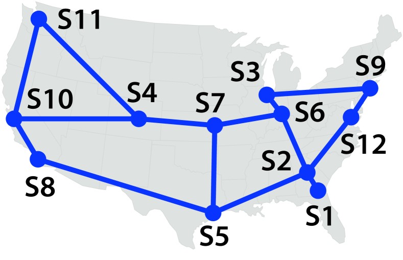
(a) Topology

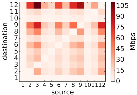
(b) Traffic matrix

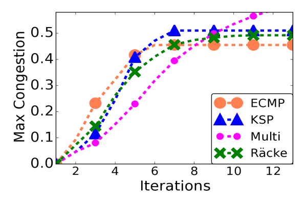
(c) Max congestion

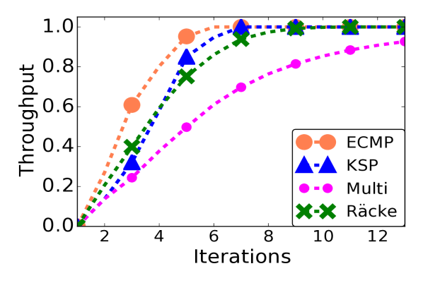
(d) Throughput

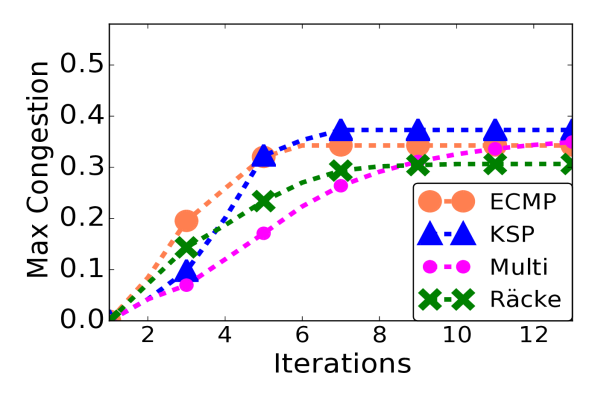
(e) Max congestion

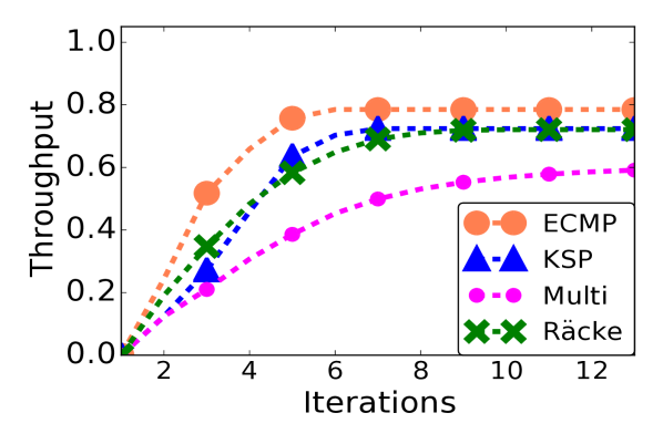
(f) Throughput

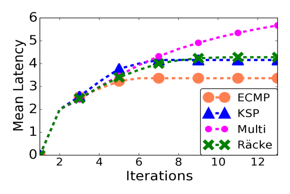
(g) Path length

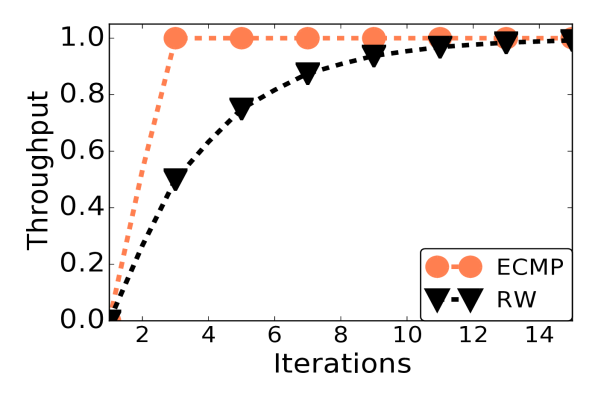
(h) Random walk

Figure 5: Case study with Abilene: (c, d) without loss. (e, f) with faulty links. (h) random walk in 4-cycle: all packets are eventually delivered.

9 Implementation and Case Studies

We built a simple interpreter for ProbNetKAT in OCaml that implements the denotational semantics as presented in Figure 2. Given a query, the interpreter approximates the answer through a monotonically increasing sequence of values (Theorems 22 and 23). Although preliminary in nature—more work on data structures and algroithms for manipulating distributions would be needed to obtain an efficient implementation—we were able to use our implementation to conduct several case studies involving probabilistic reasoning about properties of a real-world network: Internet2’s Abilene backbone.

Routing.

In the networking literature, a large number of traffic engineering (TE) approaches have been explored. We built ProbNetKAT implementations of each of the following routing schemes:

• Equal Cost Multipath Routing (ECMP): The network uses all least-cost paths between each source-destination pair, and maps incoming traffic flows onto those paths randomly. ECMP can reduce congestion and increase throughput, but can also perform poorly when multiple paths traverse the same bottleneck link.

• $k$-Shortest Paths (KSP): The network uses the top $k$-shortest paths between each pair of hosts, and again maps incoming traffic flows onto those paths randomly. This approach inherits the benefits of ECMP and provides improved fault-tolerance properties since it always spreads traffic across $k$ distinct paths.

• Multipath Routing (Multi): This is similar to KSP, except that it makes an independent choice from among the $k$-shortest paths at each hop rather than just once at ingress. This approach dynamically routes around bottlenecks and failures but can use extremely long paths—even ones containing loops.

• Oblivious Routing (Räcke): The network forwards traffic using a pre-computed probability distribution on carefully constructed overlays. The distribution is constructed in such a way that guarantees worst-case congestion within a polylogarithmic factor of the optimal scheme, regardless of the demands for traffic.

Note that all of these schemes rely on some form of randomization and hence are probabilistic in nature.

Traffic Model.

Network operators often use traffic models constructed from historical data to predict future performance. We built a small OCaml tool that translates traffic models into ProbNetKAT programs using a simple encoding. Assume that we are given a traffic matrix (TM) that relates pairs of hosts $(u,v)$ to the amount of traffic that will be sent from $u$ to $v$. By normalizing each TM entry using the aggregate demand $\sum_{(u,v)}TM(u,v)$, we get a probability distribution $d$ over pairs of hosts. For a pair of source and destination $(u,v)$, the associated probability $d(u,v)$ denotes the amount of traffic from $u$ to $v$ relative to the total traffic. Assuming uniform packet sizes, this is also the probability that a random packet generated in the network has source $u$ and destination $v$. So, we can encode a TM as a program that generates packets according to $d$:

$$inp \triangleq~{}\scalebox{2.0}{$\oplus$}_{d(u,v)}\pi_{(u,v)}!$$

$$\mbox{where, }\pi_{(u,v)}! \triangleq\mathsf{src}\kern 0.43057pt{\leftarrow}\kern 0.43057ptu\mathbin{;}\mathsf{dst}\kern 0.43057pt{\leftarrow}\kern 0.43057ptv\mathbin{;}\mathsf{sw}\kern 0.43057pt{\leftarrow}\kern 0.43057ptu$$

$\pi_{(u,v)}!$ generates a packet at $u$ with source $u$ and destination $v$. For any (non-empty) input, $inp$ generates a distribution $\mu$ on packet histories which can be fed to the network program. For instance, consider a uniform traffic distribution for our 4-switch example (see Figure 1) where each node sends equal traffic to every other node. There are twelve $(u,v)$ pairs with $u\neq v$. So, $d(u,v)_{u\neq v}=\frac{1}{12}$ and $d(u,u)=0$. We also store the aggregate demand as it is needed to model queries such as expected link congestion, throughput etc.

Queries.

Our implementation can be used to answer probabilistic queries about a variety of network performance properties. §2 showed an example of using a query to compute expected congestion. We can also measure expected mean latency in terms of path length:

⬇

let path_length (h:Hist.t) : Real.t =

Real.of_int ((Hist.length h)/2 + 1)

let lift_query_avg

(q:Hist.t -> Real.t) : (HSet.t -> Real.t) =

fun hset ->

let n = HSet.length hset in

if n = 0 then Real.zero else

let sum = HSet.fold hset $\scriptstyle\mathtt{\sim}$init:Real.zero

$\scriptstyle\mathtt{\sim}$f:(fun acc h -> Real.(acc + q h)) in

Real.(sum / of_int n)

The latency function (path_length) counts the number of switches in a history. We lift this function to sets and compute the expectation (lift_query_avg) by computing the average over all histories in the set (after discarding empty sets).

Case Study: Abilene.

To demonstrate the applicability of ProbNetKAT for reasoning about a real network, we performed a case study based on the topology and traffic demands from Internet2’s Abilene backbone network as shown in Figure 5 (a). We evaluate the traffic engineering approaches discussed above by modeling traffic matrices based on NetFlow traces gathered from the production network. A sample TM is depicted in Figure 5 (b).

Figures 5 (c,d,g) show the expected maximum congestion, throughput and mean latency. Because we model a network using the Kleene star operator, we see that the values converge monotonically as the number of iterations used to approximate Kleene star increases, as guaranteed by Corollary 23.

Failures.

Network failures such as a faulty router or a link going down are common in large networks Gill et al. [2011]. Hence, it is important to be able to understand the behavior and performance of a network in the presence of failures. We can model failures by assigning empirically measured probabilities to various components—e.g., we can modify our encoding of the topology so that every link in the network drops packets with probability $\frac{1}{10}$:

$$\begin{array}[]{rcl}\ell_{1,2}&\mathrel{\smash{\triangleq}}&{\mathsf{sw}\kern 0.43057pt{=}\kern 0.43057ptS_{1}\mathbin{;}\mathsf{pt}\kern 0.43057pt{=}\kern 0.43057pt2\mathbin{;}\mathsf{dup}}\mathbin{;}(({\mathsf{sw}\kern 0.43057pt{\leftarrow}\kern 0.43057ptS_{2}\mathbin{;}\mathsf{pt}\kern 0.43057pt{\leftarrow}\kern 0.43057pt1\mathbin{;}\mathsf{dup}})\oplus_{0.9}0)\\ &\mathbin{\&}&{\mathsf{sw}\kern 0.43057pt{=}\kern 0.43057ptS_{2}\mathbin{;}\mathsf{pt}\kern 0.43057pt{=}\kern 0.43057pt1\mathbin{;}\mathsf{dup}}\mathbin{;}(({\mathsf{sw}\kern 0.43057pt{\leftarrow}\kern 0.43057ptS_{1}\mathbin{;}\mathsf{pt}\kern 0.43057pt{\leftarrow}\kern 0.43057pt2\mathbin{;}\mathsf{dup}})\oplus_{0.9}0)\end{array}$$

Figures 5 (e-f) show the network performance for Abilene under this failure model. As expected, congestion and throughput decrease as more packets are dropped. As every link drops packets probabilistically, the relative fraction of packets delivered using longer links decreases—hence, there is a decrease in mean latency.

Loop detection.

Forwarding loops in a network are extremely undesirable as they increase congestion and can even lead to black holes. With probabilistic routing, not all loops will necessarily result in a black hole—if there is a non-zero probability of exiting a loop, every packet entering it will eventually exit. Consider the example of random walk routing in the four-node topology from Figure 1. In a random walk, a switch either forwards traffic directly to its destination or to a random neighbor. As packets are never duplicated and only exit the network when they reach their destination, the total throughput is equivalent to the fraction of packets that exit the network. Figure 5 (h) shows that the fraction of packets exiting increases monotonically with number of iterations and converges to $1$. Moreover, histories can be queried to test if it encountered a topological loop by checking for duplicate locations. Hence, given a model that computes all possible history prefixes that appear in the network, we can query it for presence of loops. We do this by removing $\mathit{out}$ from our standard network model and using $\mathit{in}\mathbin{;}(p\mathbin{;}t)^{*}\mathbin{;}p$ instead. This program generates the required distribution on history prefixes. Moreover, if we generalize packets with wildcard fields, similar to HSA Kazemian et al. [2012], we can check for loops symbolically. We have extended our implementation in this way, and used it to check whether the network exhibits loops on a number of routing schemes based on probabilistic forwarding.

10 Related Work

This paper builds on previous work on NetKAT Anderson et al. [2014]; Foster et al. [2015] and ProbNetKAT Foster et al. [2016], but develops a semantics based on ordered domains as well as new applications to traffic engineering.

Domain Theory.

The domain-theoretic treatment of probability measures goes back to the seminal work of Saheb-Djahromi Saheb-Djahromi [1980], who was the first to identify and study the CPO of probability measures. Jones and Plotkin Jones and Plotkin [1989]; Jones [1989] generalized and extended this work by giving a category-theoretical treatment and proving that the probabilistic powerdomain is a monad. It is an open problem if there exists a cartesian-closed category of continuous DCPOs that is closed under the probabilistic powerdomain; see Jung and Tix [1998] for a discussion. This is an issue for higher-order probabilistic languages, but not for ProbNetKAT, which is strictly first-order. Edalat Edalat [1994, 1996]; Edalat and Heckmann [1998] gives a computational account of measure theory and integration for general metric spaces based on domain theory. More recent papers on probabilistic powerdomains are Jung and Tix [1998]; Heckmann [1994]; Graham [1988]. All this work is ultimately based on Scott’s pioneering work Scott [1972].

Probabilistic Logic and Semantics.

Computational models and logics for probabilistic programming have been extensively studied. Denotational and operational semantics for probabilistic while programs were first studied by Kozen Kozen [1981]. Early logical systems for reasoning about probabilistic programs were proposed in Kozen [1985]; Ramshaw [1979]; Saheb-Djahromi [1978]. There are also numerous recent efforts Gordon et al. [2014]; Gretz et al. [2015]; Kozen et al. [2013]; Larsen et al. [2012]; Morgan et al. [1996]. Sankaranarayanan et al. Sankaranarayanan et al. [2013] propose static analysis to bound the the value of probability queries. Probabilistic programming in the context of artificial intelligence has also been extensively studied in recent years Borgström et al. [2011]; Roy [2011]. Probabilistic automata in several forms have been a popular model going back to the early work of Paz Paz [1971], as well as more recent efforts McIver et al. [2008]; Segala [2006]; Segala and Lynch [1995]. Denotational models combining probability and nondeterminism have been proposed by several authors McIver and Morgan [2004]; Tix et al. [2009]; Varacca and Winskel [2006], and general models for labeled Markov processes, primarily based on Markov kernels, have been studied extensively Doberkat [2007]; Panangaden [1998, 2009].

Our semantics is also related to the work on event structures Nielsen et al. [1979]; Varacca et al. [2006]. A (Prob)NetKAT program denotes a simple (probabilistic) event structure: packet histories are events with causal dependency given by extension and with all finite subsets consistent. We have to yet explore whether the event structure perspective on our semantics could lead to further applications and connections to e.g. (concurrent) games.

Networking.

Network calculus is a general framework for analyzing network behavior using tools from queuing theory Cruz. [1991]. It has been used to reason about quantitative properties such as latency, bandwidth, and congestion. The stochastic branch of network calculus provides tools for reasoning about the probabilistic behavior, especially in the presence of statistical multiplexing, but is often considered difficult to use. In contrast, ProbNetKAT is a self-contained framework based on a precise denotational semantics.

Traffic engineering has been extensively studied and a wide variety of approaches have been proposed for data-center networks Al-Fares et al. [2010]; Jeyakumar et al. [2013]; Perry et al. [2014]; Zhang-Shen and McKeown [2005]; Shieh et al. [2010] and wide-area networks Hong et al. [2013]; Jain et al. [2013]; Fortz et al. [2002]; Applegate and Cohen [2003]; Räcke [2008]; Kandula et al. [2005]; Suchara et al. [2011]; He and Rexford [2008]. These approaches optimize for metrics such as congestion, throughput, latency, fault tolerance, fairness etc. Optimal techniques typically have high overheads Danna et al. [2012], but oblivious Kodialam et al. [2009]; Applegate and Cohen [2003] and hybrid approaches with near-optimal performance Hong et al. [2013]; Jain et al. [2013] have recently been adopted.

11 Conclusion

This paper presents a new order-theoretic semantics for ProbNetKAT in the style of classical domain theory. The semantics allows a standard least-fixpoint treatment of iteration, and enables new modes of reasoning about the probabilistic network behavior. We have used these theoretical tools to analyze several randomized routing protocols on real-world data.

The main technical insight is that all programs and the operators defined on them are continuous, provided we consider the right notion of continuity: that induced by the Scott topology. Continuity enables precise approximation, and we exploited this to build an implementation. But continuity is also a powerful tool for reasoning that we expect to be very helpful in the future development of ProbNetKAT’s meta theory. To establish continuity we had to switch from the Cantor to the Scott topology, and give up reasoning in terms of a metric. Luckily we were able to show a strong correspondence between the two topologies and that the Cantor-perspective and the Scott-perspective lead to equivalent definitions of the semantics. This allows us to choose whichever perspective is best-suited for the task at hand.

Future Work.

The results of this paper are general enough to accommodate arbitrary extensions of ProbNetKAT with continuous Markov kernels or continuous operators on such kernels. An obvious next step is therefore to investigate extension of the language that would enable richer network models. Previous work on deterministic NetKAT included a decision procedure and a sound and complete axiomatization. In the presence of probabilities we expect a decision procedure will be hard to devise, as witnessed by several undecidability results on probabilistic automata. We intend to explore decision procedures for restricted fragments of the language. Another interesting direction is to compile ProbNetKAT programs into suitable automata that can then be analyzed by a probabilistic model checker such as PRISM Kwiatkowska et al. [2011]. A sound and complete axiomatization remains subject of further investigation, we can draw inspiration from recent work Kozen et al. [2013]; Mardare et al. [2016]. Another opportunity is to investigate a weighted version of NetKAT, where instead of probabilities we consider weights from an arbitrary semiring, opening up several other applications—e.g. in cost analysis. Finally, we would like to explore efficient implementation techniques including compilation, as well as approaches based on sampling, following several other probabilistic languages Park et al. [2008]; Borgström et al. [2011].

The authors wish to thank Arthur Azevedo de Amorim, David Kahn, Anirudh Sivaraman, Hongseok Yang, the Cornell PLDG, and the Barbados Crew for insightful discussions and helpful comments. Our work is supported by the National Security Agency; the National Science Foundation under grants CNS-1111698, CNS-1413972, CCF-1422046, CCF-1253165, and CCF-1535952; the Office of Naval Research under grant N00014-15-1-2177; the European Research Council under starting grant ProFoundNet (679127); a Leverhulme Prize (PLP-2016-129); and gifts from Cisco, Facebook, Google, and Fujitsu.

Appendix A $(\mathcal{M},\sqsubseteq)$ is not a Semilattice

Despite the fact that $(\mathcal{M},\sqsubseteq)$ is a directed set (Lemma 12), it is not a semilattice. Here is a counterexample.

Let $b=\{\pi,\sigma,\tau\}$, where $\pi$, $\sigma$, $\tau$ are distinct packets. Let

$$\mu_{1}=\tfrac{1}{2}\delta_{\{\pi\}}+\tfrac{1}{2}\delta_{\{\sigma\}}\qquad\mu_{2}=\tfrac{1}{2}\delta_{\{\sigma\}}+\tfrac{1}{2}\delta_{\{\tau\}}$$

$$\mu_{3}=\tfrac{1}{2}\delta_{\{\tau\}}+\tfrac{1}{2}\delta_{\{\pi\}}.$$

The measures $\mu_{1}$, $\mu_{2}$, $\mu_{3}$ would be the output measures of the programs $\pi!\oplus\sigma!$, $\sigma!\oplus\tau!$, $\tau!\oplus\pi!$, respectively.

We claim that $\mu_{1}\sqcup\mu_{2}$ does not exist. To see this, define

$$\nu_{1}=\tfrac{1}{2}\delta_{\{\tau\}}+\tfrac{1}{2}\delta_{\{\pi,\sigma\}}\qquad\nu_{2}=\tfrac{1}{2}\delta_{\{\pi\}}+\tfrac{1}{2}\delta_{\{\sigma,\tau\}}$$

$$\nu_{3}=\tfrac{1}{2}\delta_{\{\sigma\}}+\tfrac{1}{2}\delta_{\{\tau,\pi\}}.$$

All $\nu_{i}$ are $\sqsubseteq$-upper bounds for all $\mu_{j}$. (In fact, any convex combination $r\nu_{1}+s\nu_{2}+t\nu_{3}$ for $0\leq r,s,t$ and $r+s+t=1$ is an upper bound for any convex combination $u\mu_{1}+v\mu_{2}+w\mu_{3}$ for $0\leq u,v,w$ and $u+v+w=1$.) But we show by contradiction that there cannot exist a measure that is both $\sqsubseteq$-above $\mu_{1}$ and $\mu_{2}$ and $\sqsubseteq$-below $\nu_{1}$ and $\nu_{2}$. Suppose $\rho$ was such a measure. Since $\rho\sqsubseteq\nu_{1}$ and $\rho\sqsubseteq\nu_{2}$, we have

$$\rho(B_{\sigma\tau})\leq\nu_{1}(B_{\sigma\tau})=0\qquad\rho(B_{\tau\pi})\leq\nu_{1}(B_{\tau\pi})=0$$

$$\rho(B_{\pi\sigma})\leq\nu_{2}(B_{\pi\sigma})=0.$$

Since $\mu_{1}\sqsubseteq\rho$ and $\mu_{2}\sqsubseteq\rho$, we have

$$\rho(B_{\pi})\geq\mu_{1}(B_{\pi})=\tfrac{1}{2}\qquad\rho(B_{\sigma})\geq\mu_{1}(B_{\sigma})=\tfrac{1}{2}$$

$$\rho(B_{\tau})\geq\mu_{2}(B_{\tau})=\tfrac{1}{2}.$$

But then

$$\rho(A_{\pi b}) =\rho(B_{\pi})-\rho(B_{\pi\sigma}\cup B_{\tau\pi})\geq\tfrac{1}{2}$$

$$\rho(A_{\sigma b}) =\rho(B_{\sigma})-\rho(B_{\sigma\tau}\cup B_{\pi\sigma})\geq\tfrac{1}{2}$$

$$\rho(A_{\tau b}) =\rho(B_{\tau})-\rho(B_{\tau\pi}\cup B_{\sigma\tau})\geq\tfrac{1}{2},$$

which is impossible, because $\rho$ would have total weight at least $\tfrac{3}{2}$.

Appendix B Non-Algebraicity

Here is a counterexample to the conjecture that the elements continuous DCPO of continuous kernels is algebraic with finite elements $b\mathbin{;}P\mathbin{;}d$. Let $\sigma,\tau$ be packets and let $\sigma!$ and $\tau!$ be the programs that set the current packet to $\sigma$ or $\tau$, respectively. For $r\in[\frac{1}{2},1]$, let $P_{r}=(\sigma!\mathrel{\oplus_{r}}\tau!)\mathbin{\&}(\tau!\mathrel{\oplus_{r}}\sigma!)$. On any nonempty input, $P_{r}$ produces $\{\sigma\}$ with probability $r(1-r)$, $\{\tau\}$ with probability $r(1-r)$, and $\{\sigma,\tau\}$ with probability $r^{2}+(1-r)^{2}$. In particular, $P_{1}$ produces $\{\sigma,\tau\}$ with probability $1$. The kernels $P_{r}$ for $1/2\leq r<1$ form a directed set whose supremum is $P_{1}$, yet $\{\sigma\}\mathbin{;}P_{1}\mathbin{;}\{\sigma,\tau\}$ is not $\sqsubseteq$-bounded by any $P_{r}$ for $r<1$, therefore the up-closure of $\{\sigma\}\mathbin{;}P_{1}\mathbin{;}\{\sigma,\tau\}$ is not an open set.

Appendix C Cantor Meets Scott

This appendix contains proofs omitted from §5.

Proof of Lemma 9.

For any $a\subseteq b$,

$$X_{a} =\mu(B_{a})=\sum_{a\subseteq c\subseteq b}\mu(A_{cb})$$

$$=\sum_{c}[a\subseteq c]\cdot[c\subseteq b]\cdot\mu(A_{cb})$$

$$=\sum_{c}E[b]_{ac}\cdot Y_{c}=(E[b]\cdot Y)_{a}.$$

∎

Proof of Theorem 10.

Given a probability measure $\mu$, certainly (i) and (ii) hold of the matrices $M$ and $N$ formed from $\mu$ by the rule (5.6). For (iii), we calculate:

$$(E^{-1}ME)_{ab}=\sum_{c,d}E^{-1}_{ac}M_{cd}E_{db}=\sum_{c,d}E^{-1}_{ac}M_{cd}E_{db}$$

$$=\sum_{c,d}[a\subseteq c]\cdot(-1)^{|c-a|}\cdot[c=d]\cdot\mu(M_{cd})\cdot[d\subseteq b]$$

$$=\sum_{a\subseteq c\subseteq b}(-1)^{|c-a|}\cdot\mu(B_{c})=\mu(A_{ab})=N_{ab}.$$

That the correspondence is one-to-one is immediate from Theorem 8. ∎

Appendix D A DCPO on Markov Kernels

This appendix contains proofs omitted from §6.

Proof of Theorem 11.

We prove the theorem for our concrete instance $(\smash{2^{\mathsf{H}}},\mathcal{B})$. The relation $\sqsubseteq$ is a partial order. Reflexivity and transitivity are clear, and antisymmetry follows from Lemma 7.

To show that suprema of directed sets exist, let $\mathcal{D}$ be a directed set of measures, and define

$$(\bigsqcup\mathcal{D})(B) \mathrel{\smash{\triangleq}}\sup_{\mu\in\mathcal{D}}\mu(B),\ B\in\mathcal{O}.$$

This is clearly the supremum of $\mathcal{D}$, provided it defines a valid measure. To show this, choose a countable chain $\mu_{0}\sqsubseteq\mu_{1}\sqsubseteq\cdots$ in $\mathcal{D}$ such that $\mu_{m}\sqsubseteq\mu_{n}$ for all $m<n$ and $(\bigsqcup\mathcal{D})(B_{c})-\mu_{n}(B_{c})\leq 1/n$ for all $c$ such that $|c|\leq n$. Then for all finite $c\in\smash{2^{\mathsf{H}}}$, $(\bigsqcup\mathcal{D})(B_{c})=\sup_{n}\mu_{n}(B_{c})$.

Then $\bigsqcup\mathcal{D}$ is a measure by Theorem 8 because for all finite $b$ and $a\subseteq b$,

$$\sum_{a\subseteq c\subseteq b}(-1)^{|c-a|}(\bigsqcup\mathcal{D})(B_{c}) =\sum_{a\subseteq c\subseteq b}(-1)^{|c-a|}\sup_{n}\mu_{n}(B_{c})$$

$$=\lim_{n}\sum_{a\subseteq c\subseteq b}(-1)^{|c-a|}\mu_{n}(B_{c})$$

$$\geq 0.$$

To show that $\delta_{\varnothing}$ is $\sqsubseteq$-minimum, observe that for all $B\in\mathcal{O}$,

$$\delta_{\varnothing}(B) =[\varnothing\in B]=[B=B_{\varnothing}=\smash{2^{\mathsf{H}}}]$$

as $B_{\varnothing}=\smash{2^{\mathsf{H}}}$ is the only up-closed set containing $\varnothing$. Thus for all measures $\mu$, $\delta_{\varnothing}(\smash{2^{\mathsf{H}}})=1=\mu(\smash{2^{\mathsf{H}}})$, and for all $B\in\mathcal{O}$, $B\neq\smash{2^{\mathsf{H}}}$, $\delta_{\varnothing}(B)=0\leq\mu(B)$.

Finally, to show that $\delta_{H}$ is $\sqsubseteq$-maximum, observe that every nonempty $B\in\mathcal{O}$ contains $H$ because it is up-closed. Therefore, $\delta_{H}$ is the constant function $1$ on $\mathcal{O}-\{\varnothing\}$, making it $\sqsubseteq$-maximum. ∎

Proof of Lemma 12.

For any up-closed measurable set $B$,

$$\mu(B) =\mu(B)\cdot\nu(\smash{2^{\mathsf{H}}})=(\mu\times\nu)(B\times\smash{2^{\mathsf{H}}})$$

$$=(\mu\times\nu)(\{(b,c)\mid b\in B\})$$

$$\leq(\mu\times\nu)(\{(b,c)\mid b\cup c\in B\})=(\mu\mathbin{\&}\nu)(B).$$

and similarly for $\nu$. ∎

Proof of Lemma 13.

To show that (i), (ii), and (iv) are equivalent,

$$\forall a\in\smash{2^{\mathsf{H}}}\ \forall B\in\mathcal{O}\ P(a,B)\leq Q(a,B)$$

$$\Leftrightarrow\forall a\in\smash{2^{\mathsf{H}}}\ (\forall B\in\mathcal{O}\ P(a,B)\leq Q(a,B))$$

$$\Leftrightarrow\forall a\in\smash{2^{\mathsf{H}}}\ P(a,-)\sqsubseteq Q(a,-)$$

$$\Leftrightarrow\forall a\in\smash{2^{\mathsf{H}}}\ (\operatorname{\mathsf{curry}}P)(a)\sqsubseteq(\operatorname{\mathsf{curry}}Q)(a)$$

$$\Leftrightarrow\operatorname{\mathsf{curry}}P\sqsubseteq\operatorname{\mathsf{curry}}Q.$$

To show that (i) and (iii) are equivalent,

$$\forall a\in\smash{2^{\mathsf{H}}}\ \forall B\in\mathcal{O}\ P(a,B)\leq Q(a,B)$$

$$\Leftrightarrow\forall B\in\mathcal{O}\ (\forall a\in\smash{2^{\mathsf{H}}}\ P(a,B)\leq Q(a,B))$$

$$\Leftrightarrow\forall B\in\mathcal{O}\ P(-,B)\sqsubseteq Q(-,B).$$

∎

Proof of Theorem 14.

We must show that the supremum of any directed set of continuous Markov kernels is a continuous Markov kernel. In general, the supremum of a directed set of continuous functions between DCPOs is continuous. Given a directed set $\mathcal{D}$ of continuous kernels, we apply this to the directed set $\{\operatorname{\mathsf{curry}}P:\smash{2^{\mathsf{H}}}\to\mathcal{M}(\smash{2^{\mathsf{H}}})\mid P\in\mathcal{D}\}$ to derive that ${\textstyle\bigsqcup}_{P\in\mathcal{D}}\operatorname{\mathsf{curry}}P$ is continuous, then use the fact that $\operatorname{\mathsf{curry}}$ is continuous to infer that ${\textstyle\bigsqcup}_{P\in\mathcal{D}}\operatorname{\mathsf{curry}}P=\operatorname{\mathsf{curry}}{\textstyle\bigsqcup}\mathcal{D}$, therefore $\operatorname{\mathsf{curry}}{\textstyle\bigsqcup}\mathcal{D}$ is continuous. This says that the function $P:\smash{2^{\mathsf{H}}}\times\mathcal{B}\to[0,1]$ is continuous in its first argument.

We must still argue that the supremum ${\textstyle\bigsqcup}\mathcal{D}$ is a Markov kernel, that is, a measurable function in its first argument and a probability measure in its second argument. The first statement follows from the fact that any continuous function is measurable with respect to the Borel sets generated by the topologies of the two spaces. For the second statement, we appeal to Theorem 11 and the continuity of $\operatorname{\mathsf{curry}}$:

$$(\operatorname{\mathsf{curry}}{\textstyle\bigsqcup}\mathcal{D})(a) =({\textstyle\bigsqcup}_{P\in\mathcal{D}}\operatorname{\mathsf{curry}}P)(a)={\textstyle\bigsqcup}_{P\in\mathcal{D}}(\operatorname{\mathsf{curry}}P)(a),$$

which is a supremum of a directed set of probability measures, therefore by Theorem 11 is itself a probability measure.

To show that it is a continuous DCPO with basis of the indicated form, we note that for any $a\in\smash{2^{\mathsf{H}}}$ and $B\in\mathcal{O}$,

$$(b\mathbin{;}P\mathbin{;}d)(a,B)=P(a\cap b,\{c\mid c\cap d\in B\}).$$ (D.9)

Every element of the space is the supremum of a directed set of such elements. Given a continuous kernel $P$, consider the directed set $\mathcal{D}$ of all elements $b\mathbin{;}P\mathbin{;}d$ for $b,d$ finite. Then for any $a\in\smash{2^{\mathsf{H}}}$ and $B\in\mathcal{O}$,

$$({\textstyle\bigsqcup}\mathcal{D})(a,B) =\sup_{b,d\in\raisebox{1.0pt}{$\wp$\kern-0.7pt}_{\omega}(\mathsf{H})}P(a\cap b,\{c\mid c\cap d\in B\})$$ (D.10)

$$=\sup_{d\in\raisebox{1.0pt}{$\wp$\kern-0.7pt}_{\omega}(\mathsf{H})}P(a,\{c\mid c\cap d\in B\})$$ (D.11)

$$=P(a,B),$$ (D.12)

the inference (D.10) from (D.9), the inference (D.11) from the fact that $P$ is continuous in its first argument, and the inference (D.11) from the fact that the sets $\{c\mid c\cap d\in B\}$ for $d\in\raisebox{1.0pt}{$\wp$\kern-0.7pt}_{\omega}(\mathsf{H})$ form a directed set of Scott-open sets whose union is $B$ and that $P$ is a measure in its second argument. ∎

Appendix E Continuity of Kernels and Program Operators and a Least-Fixpoint Characterization of Iteration

This appendix contains lemmas and proofs omitted from §7.

E.1 Products and Integration

This section develops some properties of products and integration needed for from the point of view of Scott topology.

As pointed out by Jones [Jones, 1989, §3.6], the product $\sigma$-algebra of the Borel sets of two topological spaces $X,Y$ is in general not the same as the Borel sets of the topological product $X\times Y$, although this property does hold for the Cantor space, as its basic open sets are clopen. More importantly, as also observed in [Jones, 1989, §3.6], the Scott topology on the product of DCPOs with the componentwise order is not necessarily the same as the product topology. However, in our case, the two topologies coincide.

Theorem 26.

Let $D_{\alpha}$, $\alpha<\kappa$, be a collection of algebraic DCPOs with $F_{\alpha}$ the finite elements of $D_{\alpha}$. Then the product $\prod_{\alpha<\kappa}D_{\alpha}$ with the componentwise order is an algebraic DCPO with finite elements

$$F =\{c\in\textstyle\prod_{\alpha}F_{\alpha}\mid\text{$\pi_{\alpha}(c)=\bot$ for all but finitely many $\alpha$}\}.$$

Proof.

The projections $\pi_{\beta}:\prod_{\alpha}D_{\alpha}\to D_{\beta}$ are easily shown to be continuous with respect to the componentwise order. For any $d\in\prod_{\alpha<\kappa}D_{\alpha}$, the set $\{d\}{\downarrow}\cap F$ is directed, and $d=\bigsqcup(\{d\}{\downarrow}\cap F)$: for any $\alpha$, the set $\pi_{\alpha}(\{d\}{\downarrow}\cap F)=\{\pi_{\alpha}(d)\}{\downarrow}\cap F_{\alpha}$ is directed, thus

$$\pi_{\alpha}(d) =\bigsqcup(\{\pi_{\alpha}(d)\}{\downarrow}\cap F_{\alpha})=\bigsqcup(\pi_{\alpha}(\{d\}{\downarrow}\cap F))$$

$$=\pi_{\alpha}(\bigsqcup(\{d\}{\downarrow}\cap F)),$$

and as $\alpha$ was arbitrary, $d=\bigsqcup(\{d\}{\downarrow}\cap F)$.

It remains to show that $\{c\}{\uparrow}=\prod_{\alpha<\kappa}\{\pi_{\alpha}(c)\}{\uparrow}$ is open for $c\in F$. Let $A$ be a directed set with $\bigsqcup A\in\{c\}{\uparrow}$. For each $\alpha$, $\{\pi_{\alpha}(a)\mid a\in A\}$ is directed, and

$$\bigsqcup_{a\in A}\pi_{\alpha}(a) =\pi_{\alpha}(\bigsqcup A)\in\pi_{\alpha}(\{c\}{\uparrow})=\{\pi_{\alpha}(c)\}{\uparrow},$$

so there exists $a_{\alpha}\in A$ such that $\pi_{\alpha}(a_{\alpha})\in\{\pi_{\alpha}(c)\}{\uparrow}$. Since $A$ is directed, there is a single $a\in A$ that majorizes the finitely many $a_{\alpha}$ such that $\pi_{\alpha}(c)\neq\bot$. Then $\pi_{\alpha}(a)\in\{\pi_{\alpha}(c)\}{\uparrow}$ for all $\alpha$, thus $a\in\{c\}{\uparrow}$. ∎

Corollary 27.

The Scott topology on a product of algebraic DCPOs with respect to the componentwise order coincides with the product topology induced by the Scott topology on each component.

Proof.

Let $\prod_{\alpha<\kappa}D_{\alpha}$ be a product of algebraic DCPOs with $\mathcal{O}_{0}$ the product topology and $\mathcal{O}_{1}$ the Scott topology. As noted in the proof of Theorem 26, the projections $\pi_{\beta}:\prod_{\alpha}D_{\alpha}\to D_{\beta}$ are continuous with respect to $\mathcal{O}_{1}$. By definition, $\mathcal{O}_{0}$ is the weakest topology on the product such that the projections are continuous, so $\mathcal{O}_{0}\subseteq\mathcal{O}_{1}$.

For the reverse inclusion, we use the observation that the sets $\{c\}{\uparrow}$ for finite elements $c\in F$ as defined in Theorem 26 form a base for the topology $\mathcal{O}_{1}$. These sets are also open in $\mathcal{O}_{0}$, since they are finite intersections of sets of the form $\pi_{\alpha}^{-1}(\{\pi_{\alpha}(c)\}{\uparrow})$, and $\{\pi_{\alpha}(c)\}{\uparrow}$ is open in $D_{\alpha}$ since $\pi_{\alpha}(c)\in F_{\alpha}$. As $\mathcal{O}_{1}$ is the smallest topology containing its basic open sets, $\mathcal{O}_{1}\subseteq\mathcal{O}_{0}$. ∎

A function $g:\smash{2^{\mathsf{H}}}\to\mathbb{R}_{+}$ is $\mathcal{O}$-simple if it is a finite linear combination of the form $\sum_{A\in F}r_{A}\mathbf{1}_{A}$, where $F$ is a finite subset of $\mathcal{O}$. Let $S_{\mathcal{O}}$ denote the set of $\mathcal{O}$-simple functions.

Theorem 28.

Let $f$ be a bounded Scott-continuous function $f:\smash{2^{\mathsf{H}}}\to\mathbb{R}_{+}$. Then

$$\sup_{\begin{subarray}{c}g\in S_{\mathcal{O}}\\ g\leq f\end{subarray}}\int g\,d\mu =\int f\,d\mu=\inf_{\begin{subarray}{c}g\in S_{\mathcal{O}}\\ f\leq g\end{subarray}}\int g\,d\mu$$

under Lebesgue integration.

Proof.

Let $\varepsilon>0$ and $r_{N}=\sup_{a\in\smash{2^{\mathsf{H}}}}f(a)$. Let

$$0=r_{0}<r_{1}<\cdots<r_{N}$$

such that $r_{i+1}-r_{i}<\varepsilon$, $0\leq i\leq N-1$, and set

$$A_{i}=\{a\mid f(a)>r_{i}\}=f^{-1}((r_{i},\infty))\in\mathcal{O},\ \ 0\leq i\leq N.$$

Then $A_{i+1}\subseteq A_{i}$ and

$$A_{i}-A_{i+1}=\{a\mid r_{i}<f(a)\leq r_{i+1}\}=f^{-1}((r_{i},r_{i+1}]).$$

Let

$$f_{\bullet} =\sum_{i=0}^{N-1}r_{i}\mathbf{1}_{A_{i}-A_{i+1}} f^{\bullet} =\sum_{i=0}^{N-1}r_{i+1}\mathbf{1}_{A_{i}-A_{i+1}}.$$

For $a\in A_{i}-A_{i+1}$,

$$f_{\bullet}(a) =\sum_{i=0}^{N-1}r_{i}\mathbf{1}_{A_{i}-A_{i+1}}(a)=r_{i}<f(a)$$

$$\leq r_{i+1}=\sum_{i=0}^{N-1}r_{i+1}\mathbf{1}_{A_{i}-A_{i+1}}(a)=f^{\bullet}(a),$$

and as $a$ was arbitrary, $f_{\bullet}\leq f\leq f^{\bullet}$ pointwise. Thus

$$\int f_{\bullet}\,d\mu \leq\int f\,d\mu\leq\int f^{\bullet}\,d\mu.$$

Moreover,

$$\int f^{\bullet}\,d\mu-\int f_{\bullet}\,d\mu =\sum_{i=0}^{N-1}r_{i+1}\mu(A_{i}-A_{i+1})$$

$$\qquad\qquad-\sum_{i=0}^{N-1}r_{i}\mu(A_{i}-A_{i+1})$$

$$=\sum_{i=0}^{N-1}(r_{i+1}-r_{i})\mu(A_{i}-A_{i+1})$$

$$<\varepsilon\cdot\sum_{i=0}^{N-1}\mu(A_{i}-A_{i+1})=\varepsilon\cdot\mu(\smash{2^{\mathsf{H}}})=\varepsilon,$$

so the integral is approximated arbitrarily closely from above and below by the $f^{\bullet}$ and $f_{\bullet}$. Finally, we argue that $f_{\bullet}$ and $f^{\bullet}$ are $\mathcal{O}$-simple. Using the fact that $r_{0}=0$ and $A_{N}=\varnothing$ to reindex,

$$f_{\bullet} =\sum_{i=0}^{N-1}r_{i}\mathbf{1}_{A_{i}-A_{i+1}}=\sum_{i=0}^{N-1}r_{i}\mathbf{1}_{A_{i}}-\sum_{i=0}^{N-1}r_{i}\mathbf{1}_{A_{i+1}}$$

$$=\sum_{i=0}^{N-1}r_{i+1}\mathbf{1}_{A_{i+1}}-\sum_{i=0}^{N-1}r_{i}\mathbf{1}_{A_{i+1}}=\sum_{i=0}^{N-1}(r_{i+1}-r_{i})\mathbf{1}_{A_{i+1}},$$

$$f^{\bullet} =\sum_{i=0}^{N-1}r_{i+1}\mathbf{1}_{A_{i}-A_{i+1}}=\sum_{i=0}^{N-1}r_{i+1}\mathbf{1}_{A_{i}}-\sum_{i=0}^{N-1}r_{i+1}\mathbf{1}_{A_{i+1}}$$

$$=\sum_{i=0}^{N-1}r_{i+1}\mathbf{1}_{A_{i}}-\sum_{i=0}^{N-1}r_{i}\mathbf{1}_{A_{i}}=\sum_{i=0}^{N-1}(r_{i+1}-r_{i})\mathbf{1}_{A_{i}},$$

and both functions are $\mathcal{O}$-simple since all $A_{i}$ are in $\mathcal{O}$. ∎

We can prove a stronger version of Theorem 28 that also works for functions taking on infinite value. A function $g$ is simple if it is a finite linear combination of indicator functions of the form $g=\sum_{i=1}^{k}r_{i}\mathbf{1}_{A_{i}}$, where $k\in\mathbb{N}$ and the $A_{i}$ are measurable. Let $S$ denote the set of all simple functions.

Theorem 29.

Let $f:\smash{2^{\mathsf{H}}}\to[0,\infty]$ be Scott-continuous and let $\mu$ be a probability measure. Then

$$\int f\,d\mu=\sup_{\begin{subarray}{c}g\in S_{\mathcal{O}}\\ g\leq f\end{subarray}}\int g\,d\mu$$

Proof.

It suffices to show that

$$\sup_{\begin{subarray}{c}g\in S\\ g\leq f\end{subarray}}\int g\,d\mu=\sup_{\begin{subarray}{c}g\in S_{\mathcal{O}}\\ g\leq f\end{subarray}}\int g\,d\mu$$ (E.13)

since the left side of this equation defines the integral of $f$. We trivially have

$$\sup_{\begin{subarray}{c}g\in S\\ g\leq f\end{subarray}}\int g\,d\mu\geq\sup_{\begin{subarray}{c}g\in S_{\mathcal{O}}\\ g\leq f\end{subarray}}\int g\,d\mu$$ (E.14)

because $S_{\mathcal{O}}\subseteq S$. To show the reverse inequality, let $g\in S$ with $g\leq f$ be arbitrary. We will show that there exists a family of functions $g_{\varepsilon}\in S_{\mathcal{O}}$, $\varepsilon>0$ with $g_{\varepsilon}\leq f$ such that $\int g\,d\mu-\int g_{\varepsilon}\,d\mu\leq\varepsilon$. Together with (E.14), this proves (E.13) because it implies that

$$\sup_{\begin{subarray}{c}g\in S\\ g\leq f\end{subarray}}\int g\,d\mu\leq\sup_{\begin{subarray}{c}g\in S\\ g\leq f\end{subarray}}\sup_{\varepsilon>0}\int g_{\varepsilon}\,d\mu\leq\sup_{\begin{subarray}{c}g\in S_{\mathcal{O}}\\ g\leq f\end{subarray}}\int g\,d\mu$$

Let’s turn to constructing the family of functions $g_{\varepsilon}\in S_{\mathcal{O}}$. Since $g$ is simple, we may w.l.o.g. assume that it has the form $g=\sum_{i=1}^{k}r_{i}\mathbf{1}_{A_{i}}$ with disjoint $A_{i}\in\mathcal{B}$ and $r_{1}<r_{2}<\cdots<r_{k}$. Define

$$r_{0} \mathrel{\smash{\triangleq}}\varepsilon$$

$$B_{i,\varepsilon} \mathrel{\smash{\triangleq}}f^{-1}((r_{i}-\varepsilon,\infty])\in\mathcal{O}$$

$$\beta_{i} \mathrel{\smash{\triangleq}}r_{i}-r_{i-1}$$

$$g_{\varepsilon} \mathrel{\smash{\triangleq}}\sum_{i=1}^{k}\beta_{i}\cdot\mathbf{1}_{B_{i,\varepsilon}}\in S_{\mathcal{O}}$$

Then we have $g_{\varepsilon}\leq f$ because for all $a\in\smash{2^{\mathsf{H}}}$

$$(\sum_{i=1}^{k}\beta_{i}\cdot\mathbf{1}_{B_{i,\varepsilon}})(a) =\sum_{i=1}^{k}\beta_{i}\cdot\left[a\in B_{i,\varepsilon}\right]$$

$$=\sum_{i=1}^{k}(r_{i}-r_{i-1})\cdot\left[f(a)>r_{i}-\varepsilon\right]$$

$$=\max\{r_{i}\mid 1\leq i\leq k\text{ and }f(a)>r_{i}-\varepsilon\}-r_{0}$$

$$<f(a)$$

Moreover, we have that $g-g_{\varepsilon}\leq\varepsilon$ because

$$(\sum_{i=1}^{k}\beta_{i}\cdot\mathbf{1}_{B_{i,\varepsilon}})(a) =\max\{r_{i}\mid 1\leq i\leq k\text{ and }f(a)>r_{i}-\varepsilon\}-r_{0}$$

$$\geq\max\{r_{i}\mid 1\leq i\leq k\text{ and }f(a)\geq r_{i}\}-\varepsilon$$

$$\geq\max\{r_{i}\mid 1\leq i\leq k\text{ and }g(a)=r_{i}\}-\varepsilon$$

$$=g(a)-\varepsilon$$

Thus it follows that

$$\int g\,d\mu-\int g_{\varepsilon}\,d\mu=\int(g-g_{\varepsilon})d\mu\leq\int\varepsilon\,d\mu=\varepsilon$$

∎

Proof of Theorem 15.

(i) We prove the result first for $\mathcal{O}$-simple functions. If $\mu\sqsubseteq\nu$, then for any $\mathcal{O}$-simple function $g=\sum_{A}r_{A}\mathbf{1}_{A}$,

$$\int g\,d\mu =\int\sum_{A}r_{A}\mathbf{1}_{A}\,d\mu=\sum_{A}r_{A}\mu(A)$$

$$\leq\sum_{A}r_{A}\nu(A)=\int\sum_{A}r_{A}\mathbf{1}_{A}\,d\nu=\int g\,d\nu.$$

Thus the map (7.7) is monotone. If $\mathcal{D}$ is a directed set of measures with respect to $\sqsubseteq$, then

$$\int g\,d({\textstyle\bigsqcup}\mathcal{D}) =\int\sum_{A}r_{A}\mathbf{1}_{A}\,d({\textstyle\bigsqcup}\mathcal{D})=\sum_{A}r_{A}({\textstyle\bigsqcup}\mathcal{D})(A)$$

$$=\sup_{\mu\in\mathcal{D}}\sum_{A}r_{A}\mu(A)=\sup_{\mu\in\mathcal{D}}\int\sum_{A}r_{A}\mathbf{1}_{A}\,d\mu$$

$$=\sup_{\mu\in\mathcal{D}}\int g\,d\mu.$$

Now consider an arbitrary Scott-continuous function $f:\smash{2^{\mathsf{H}}}\to[0,\infty]$. Let $S_{\mathcal{O}}$ be the family of $\mathcal{O}$-simple functions. By Theorem 29, if $\mu\sqsubseteq\nu$, we have

$$\int f\,d\mu =\sup_{\begin{subarray}{c}g\in S_{\mathcal{O}}\\ g\leq f\end{subarray}}\int g\,d\mu\leq\sup_{\begin{subarray}{c}g\in S_{\mathcal{O}}\\ g\leq f\end{subarray}}\int g\,d\nu=\int f\,d\nu,$$

and if $\mathcal{D}$ is a directed set of measures with respect to $\sqsubseteq$, then

$$\int f\,d({\textstyle\bigsqcup}\mathcal{D}) =\sup_{\begin{subarray}{c}g\in S_{\mathcal{O}}\\ g\leq f\end{subarray}}\int g\,d({\textstyle\bigsqcup}\mathcal{D})=\sup_{\begin{subarray}{c}g\in S_{\mathcal{O}}\\ g\leq f\end{subarray}}\sup_{\mu\in\mathcal{D}}\int g\,d\mu$$

$$=\sup_{\mu\in\mathcal{D}}\sup_{\begin{subarray}{c}g\in S_{\mathcal{O}}\\ g\leq f\end{subarray}}\int g\,d\mu=\sup_{\mu\in\mathcal{D}}\int f\,d\mu.$$

(ii) This just the monotone convergence theorem for Lebesgue Integration. ∎

E.2 Continuous Operations on Measures

In this section we show that certain operations on measures are continuous. These properties will be lifted to kernels as required.

Lemma 30.

For any probability measure $\mu$ on an algebraic DCPO and open set $B$, the value $\mu(B)$ is approximated arbitrarily closely from below by $\mu(C)$ for compact-open sets $C$.

Proof.

Since the sets $\{a\}{\uparrow}$ for finite $a$ form a base for the topology, and every compact-open set is a finite union of such sets, the set $\mathcal{K}(B)$ of compact-open subsets of $B$ is a directed set whose union is $B$. Then

$$\mu(B)=\mu({\textstyle\bigcup}\mathcal{K}(B))=\sup\{\mu(C)\mid C\in\mathcal{K}(B)\}.$$

∎

Lemma 31.

The product operator on measures in algebraic DCPOs is Scott-continuous in each argument.

Proof.

The difficult part of the argument is monotonicity. Once we have that, then for any $B,C\in\mathcal{O}$, we have $(\mu\times\nu)(B\times C)=\mu(B)\cdot\nu(C)$. Thus for any directed set $D$ of measures,

$$({\textstyle\bigsqcup}D\times\nu)(B\times C)$$

$$=({\textstyle\bigsqcup}D)(B)\cdot\nu(C)=(\sup_{\mu\in D}\mu(B))\cdot\nu(C)$$

$$=\sup_{\mu\in D}(\mu(B)\cdot\nu(C))=\sup_{\mu\in D}((\mu\times\nu)(B\times C))$$

$$=({\textstyle\bigsqcup}_{\mu\in D}(\mu\times\nu))(B\times C).$$

By Theorem 26, the sets $B\times C$ for $B,C\in\mathcal{O}$ form a basis for the Scott topology on the product space $\smash{2^{\mathsf{H}}}\times\smash{2^{\mathsf{H}}}$, thus ${\textstyle\bigsqcup}D\times\nu={\textstyle\bigsqcup}_{\mu\in D}(\mu\times\nu)$.

To show monotonicity, we use approximability by compact-open sets (Lemma 30). We wish to show that if $\mu_{1}\sqsubseteq\mu_{2}$, then $\mu_{1}\times\nu\sqsubseteq\mu_{2}\times\nu$. By Lemma 30, it suffices to show that

$$(\mu_{1}\times\nu)(\bigcup_{n}B_{n}\times C_{n})\leq(\mu_{2}\times\nu)(\bigcup_{n}B_{n}\times C_{n}),$$

where the index $n$ ranges over a finite set, and $B_{n}$ and $C_{n}$ are open sets of the component spaces. Consider the collection of all atoms $A$ of the Boolean algebra generated by the $C_{n}$. For each such atom $A$, let

$$N(A) =\{n\mid\text{$C_{n}$ occurs positively in $A$}\}.$$

Then

$$\bigcup_{n}B_{n}\times C_{n} =\bigcup_{A}(\bigcup_{n\in N(A)}B_{n})\times A.$$

The right-hand side is a disjoint union, since the $A$ are pairwise disjoint. Then

$$(\mu_{1}\times\nu)(\bigcup_{n}B_{n}\times C_{n}) =(\mu_{1}\times\nu)(\bigcup_{A}(\bigcup_{n\in N(A)}B_{n})\times A)$$

$$=\sum_{A}(\mu_{1}\times\nu)((\bigcup_{n\in N(A)}B_{n})\times A)$$

$$=\sum_{A}\mu_{1}(\bigcup_{n\in N(A)}B_{n})\cdot\nu(A)$$

$$\leq\sum_{A}\mu_{2}(\bigcup_{n\in N(A)}B_{n})\cdot\nu(A)$$

$$=(\mu_{2}\times\nu)(\bigcup_{n}B_{n}\times C_{n}).$$

∎

Let $S$ and $T$ be measurable spaces and $f:S\to T$ a measurable function. For a measure $\mu$ on $S$, the push-forward measure $f_{*}(\mu)$ is the measure $\mu\circ f^{-1}$ on $T$.

Lemma 32.

If $f:(\smash{2^{\mathsf{H}}})^{\kappa}\to\smash{2^{\mathsf{H}}}$ is Scott-continuous with respect to the subset order, then the push-forward operator $f_{*}:\mathcal{M}((\smash{2^{\mathsf{H}}})^{\kappa})\to\mathcal{M}(\smash{2^{\mathsf{H}}})$ is Scott-continuous with respect to $\sqsubseteq$.

Proof.

Let $\mu,\nu\in\mathcal{M}((\smash{2^{\mathsf{H}}})^{\kappa})$, $\mu\sqsubseteq\nu$. If $B\in\mathcal{O}$, then $f^{-1}(B)$ is Scott-open in $(\smash{2^{\mathsf{H}}})^{\kappa}$, so $f_{*}(\mu)(B)=\mu(f^{-1}(B))\leq\nu(f^{-1}(B))=f_{*}(\nu)(B)$. As $B\in\mathcal{O}$ was arbitrary, $f_{*}(\mu)\sqsubseteq f_{*}(\nu)$. Similarly, if $D$ is any $\sqsubseteq$-directed set in $\mathcal{M}((\smash{2^{\mathsf{H}}})^{\kappa})$, then so is $\{f_{*}(\mu)\mid\mu\in D\}$, and

$$f_{*}({\textstyle\bigsqcup}D)(B) =({\textstyle\bigsqcup}D)(f^{-1}(B))=\sup_{\mu\in D}\mu(f^{-1}(B))$$

$$=\sup_{\mu\in D}f_{*}(\mu)(B)=({\textstyle\bigsqcup}_{\mu\in D}f_{*}(\mu))(B)$$

for any $B\in\mathcal{O}$, thus $f_{*}({\textstyle\bigsqcup}D)={\textstyle\bigsqcup}_{\mu\in D}f_{*}(\mu)$. ∎

Lemma 33.

Parallel composition of measures ($\mathbin{\&}$) is Scott-continuous in each argument.

Proof.

By definition, $\mu\mathbin{\&}\nu=(\mu\times\nu)\mathbin{;}{{\textstyle\bigcup}}^{-1}$, where ${\textstyle\bigcup}:\smash{2^{\mathsf{H}}}\times\smash{2^{\mathsf{H}}}\to\smash{2^{\mathsf{H}}}$ is the set union operator. The set union operator is easily shown to be continuous with respect to the Scott topologies on $\smash{2^{\mathsf{H}}}\times\smash{2^{\mathsf{H}}}$ and the $\smash{2^{\mathsf{H}}}$. By Lemma 32, the push-forward operator with respect to union is Scott-continuous with respect to $\sqsubseteq$. By Lemma 31, the product operator is Scott-continuous in each argument with respect to $\sqsubseteq$. The operator $\mathbin{\&}$ is the composition of these two Scott continuous operators, therefore is itself Scott-continuous. ∎

E.3 Continuous Kernels

Lemma 34.

The deterministic kernel associated with any Scott-continuous function $f:D\to E$ is a continuous kernel.

Proof.

Recall from Foster et al. [2016] that deterministic kernels are those whose output measures are Dirac measures (point masses). Any measurable function $f:D\to E$ uniquely determines a deterministic kernel $P_{f}$ such that $P_{f}(a,-)=\delta_{f(a)}$ (or equivalently, $P=\eta\circ f$) and vice versa (this was shown in Foster et al. [2016] for $D=E=\smash{2^{\mathsf{H}}}$). We show that if in addition $f$ is Scott-continuous, then the kernel $P_{f}$ is continuous.

Let $f:D\to E$ be Scott-continuous. For any open $B$, if $a\sqsubseteq b$, then $f(a)\sqsubseteq f(b)$ since $f$ is monotone. Since $B$ is up-closed, if $f(a)\in B$, then $f(b)\in B$. Thus

$$P_{f}(a,B)=[f(a)\in B]\leq[f(b)\in B]=P_{f}(b,B).$$

If $A\subseteq D$ is a directed set, then $f(\bigsqcup A)=\bigsqcup_{a\in A}f(a)$. Since $B$ is open, $\bigsqcup_{a\in A}f(a)\in B$ iff there exists $a\in A$ such that $f(a)\in B$. Then

$$P_{f}({\textstyle\bigsqcup}A,B) =[f({\textstyle\bigsqcup}A)\in B]=[{\textstyle\bigsqcup}_{a\in A}f(a)\in B]$$

$$=\sup_{a\in A}[f(a)\in B]=\sup_{a\in A}P_{f}(a,B).$$

∎

Lemma 35.

All atomic ProbNetKAT programs (including predicates) denote deterministic and Scott-continuous kernels.

Proof.

By Lemma 3, all atomic programs denote kernels of the form $a\mapsto\eta(\{f(\mathit{h})\mid\mathit{h}\in a\})$, where $f$ is a partial function $H\rightharpoonup H$. Hence they are deterministic. Using Lemma 34, we see that they are also Scott-continuous:

• If $a\subseteq b$, then $\{f(\mathit{h})\mid\mathit{h}\in a\}\subseteq\{f(\mathit{h})\mid\mathit{h}\in b\}$; and

• If $D\subseteq\smash{2^{\mathsf{H}}}$ is a directed set, then $\{f(\mathit{h})\mid\mathit{h}\in{\textstyle\bigcup}D\}=\bigcup_{a\in D}\{f(\mathit{h})\mid\mathit{h}\in a\}$.

∎

Lemma 36.

Let $P$ be a continuous Markov kernel and $f:\smash{2^{\mathsf{H}}}\to\mathbb{R}_{+}$ a Scott-continuous function. Then the map

$$a\mapsto\int_{c\in\smash{2^{\mathsf{H}}}}f(c)\cdot P(a,dc)$$ (E.15)

is Scott-continuous.

Proof.

The map (E.15) is the composition of the maps

$$a \mapsto P(a,-) P(a,-)\mapsto\int_{c\in\smash{2^{\mathsf{H}}}}P(a,dc)\cdot f(c),$$

which are Scott-continuous by Lemmas 44 and 15, respectively, and the composition of Scott-continuous maps is Scott-continuous. ∎

Lemma 37.

Product preserves continuity of Markov kernels: If $P$ and $Q$ are continuous, then so is $P\times Q$.

Proof.

We wish to show that if $a\subseteq b$, then $(P\times Q)(a,-)\sqsubseteq(P\times Q)(b,-)$, and if $A$ is a directed subset of $\smash{2^{\mathsf{H}}}$, then $(P\times Q)(\bigcup A)=\sup_{a\in A}(P\times Q)(a,-)$. For the first statement, using Lemma 31 twice,

$$(P\times Q)(a,-) =P(a,-)\times Q(a,-)\sqsubseteq P(b,-)\times Q(a,-)$$

$$\sqsubseteq P(b,-)\times Q(b,-)=(P\times Q)(b,-).$$

For the second statement, for $A$ a directed subset of $\smash{2^{\mathsf{H}}}$,

$$(P\times Q)({\textstyle\bigsqcup}A,-) =P({\textstyle\bigsqcup}A,-)\times Q({\textstyle\bigsqcup}A,-)$$

$$=({\textstyle\bigsqcup}_{a\in A}P(a,-))\times({\textstyle\bigsqcup}_{b\in A}Q(b,-))$$

$$={\textstyle\bigsqcup}_{a\in A}{\textstyle\bigsqcup}_{b\in A}P(a,-)\times Q(b,-)$$

$$={\textstyle\bigsqcup}_{a\in A}P(a,-)\times Q(a,-)$$

$$={\textstyle\bigsqcup}_{a\in A}(P\times Q)(a,-).$$

∎

Lemma 38.

Sequential composition preserves continuity of Markov kernels: If $P$ and $Q$ are continuous, then so is $P\mathbin{;}Q$.

Proof.

We have

$$(P\mathbin{;}Q)(a,A) =\int_{c\in\smash{2^{\mathsf{H}}}}P(a,dc)\cdot Q(c,A).$$

Since $Q$ is a continuous kernel, it is Scott-continuous in its first argument, thus so is $P\mathbin{;}Q$ by Lemma 36. ∎

Lemma 39.

Parallel composition preserves continuity of Markov kernels: If $P$ and $Q$ are continuous, then so is $P\mathbin{\&}Q$.

Proof.

Suppose $P$ and $Q$ are continuous. By definition, $P\mathbin{\&}Q=(P\times Q)\mathbin{;}{\textstyle\bigcup}$. By Lemma 37, $P\times Q$ is continuous, and ${\textstyle\bigcup}:\smash{2^{\mathsf{H}}}\times\smash{2^{\mathsf{H}}}\to\smash{2^{\mathsf{H}}}$ is continuous. Thus their composition is continuous by Lemma 38. ∎

Lemma 40.

The probabilistic choice operator ($\mathrel{\oplus_{r}}$) preserves continuity of kernels.

Proof.

If $P$ and $Q$ are continuous, then $P\mathrel{\oplus_{r}}Q=rP+(1-r)Q$. If $a\subseteq b$, then

$$(P\mathrel{\oplus_{r}}Q)(a,-) =rP(a,-)+(1-r)Q(a,-)$$

$$\leq rP(b,-)+(1-r)Q(b,-)$$

$$=(P\mathrel{\oplus_{r}}Q)(b,-).$$

If $A\subseteq\smash{2^{\mathsf{H}}}$ is a directed set, then

$$(P\mathrel{\oplus_{r}}Q)({\textstyle\bigcup}A,-) =rP({\textstyle\bigcup}A,-)+(1-r)Q({\textstyle\bigcup}A,-)$$

$$={\textstyle\bigsqcup}_{a\in A}(rP(a,-)+(1-r)Q(a,-))$$

$$={\textstyle\bigsqcup}_{a\in A}(P\mathrel{\oplus_{r}}Q)(a,-).$$

∎

Lemma 41.

The iteration operator (*) preserves continuity of kernels.

Proof.

Suppose $P$ is continuous. It follows inductively using Lemmas 39 and 38 that $P^{(n)}$ is continuous. Since $P^{*}=\bigsqcup_{n}P^{(n)}$ and since the supremum of a directed set of continuous kernels is continuous by Theorem 14, $P^{*}$ is continuous. ∎

Proof of Theorem 16.

The result follows from Lemmas 34, 36, 37, 38, 39, 40, and 41. ∎

Proof of Corollary 17.

This follows from Theorem 16. All primitive programs are deterministic, thus give continuous kernels, and continuity is preserved by all the program operators. ∎

E.4 Continuous Operations on Kernels

Lemma 42.

The product operation on kernels ($\times$) is Scott-continuous in each argument.

Proof.

We use Lemma 31. If $P_{1}\sqsubseteq P_{2}$, then for all $a\in\smash{2^{\mathsf{H}}}$,

$$(P_{1}\times Q)(a,-) =P_{1}(a,-)\times Q(a,-)$$

$$\sqsubseteq P_{2}(a,-)\times Q(a,-)=(P_{2}\times Q)(a,-).$$

Since $a$ was arbitrary, $P_{1}\times Q\sqsubseteq P_{2}\times Q$. For a directed set $\mathcal{D}$ of kernels,

$$({\textstyle\bigsqcup}\mathcal{D}\times Q)(a,-) =({\textstyle\bigsqcup}\mathcal{D})(a,-)\times Q(a,-)$$

$$={\textstyle\bigsqcup}_{P\in\mathcal{D}}P(a,-)\times Q(a,-)$$

$$={\textstyle\bigsqcup}_{P\in\mathcal{D}}(P(a,-)\times Q(a,-))$$

$$={\textstyle\bigsqcup}_{P\in\mathcal{D}}(P\times Q)(a,-)$$

$$=({\textstyle\bigsqcup}_{P\in\mathcal{D}}(P\times Q))(a,-).$$

Since $a$ was arbitrary, ${\textstyle\bigsqcup}\mathcal{D}\times Q={\textstyle\bigsqcup}_{P\in\mathcal{D}}(P\times Q)$. ∎

Lemma 43.

Parallel composition of kernels ($\mathbin{\&}$) is Scott-continuous in each argument.

Proof.

By definition, $P\mathbin{\&}Q=(P\times Q)\mathbin{;}{\textstyle\bigcup}$. By Lemmas 42 and 45, the product operation and sequential composition are continuous in both arguments, thus their composition is. ∎

Lemma 44.

Let $P$ be a continuous Markov kernel. The map $\operatorname{\mathsf{curry}}P$ is Scott-continuous with respect to the subset order on $\smash{2^{\mathsf{H}}}$ and the order $\sqsubseteq$ on $\mathcal{M}(\smash{2^{\mathsf{H}}})$.

Proof.

We have $(\operatorname{\mathsf{curry}}P)(a)=P(a,-)$. Since $P$ is monotone in its first argument, if $a\subseteq b$ and $B\in\mathcal{O}$, then $P(a,B)\leq P(b,B)$. As $B\in\mathcal{O}$ was arbitrary,

$$(\operatorname{\mathsf{curry}}P)(a) =P(a,-)\sqsubseteq P(b,-)=(\operatorname{\mathsf{curry}}P)(b).$$

This shows that $\operatorname{\mathsf{curry}}P$ is monotone.

Let $D\subseteq\smash{2^{\mathsf{H}}}$ be a directed set. By the monotonicity of $\operatorname{\mathsf{curry}}P$, so is the set $\{(\operatorname{\mathsf{curry}}P)(a)\mid a\in D\}$. Then for any $B\in\mathcal{O}$,

$$(\operatorname{\mathsf{curry}}P)({\textstyle\bigcup}D)(B) =P({\textstyle\bigcup}D,B)=\sup_{a\in D}P(a,B)$$

$$=\sup_{a\in D}(\operatorname{\mathsf{curry}}P)(a)(B)$$

$$=({\textstyle\bigsqcup}_{a\in D}(\operatorname{\mathsf{curry}}P)(a))(B),$$

thus $(\operatorname{\mathsf{curry}}P)({\textstyle\bigcup}D)={\textstyle\bigsqcup}_{a\in D}(\operatorname{\mathsf{curry}}P)(a)$. ∎

Lemma 45.

Sequential composition of kernels is Scott-continuous in each argument.

Proof.

To show that $\mathbin{;}$ is continuous in its first argument, we wish to show that if $P_{1},P_{2},Q$ are any continuous kernels with $P_{1}\sqsubseteq P_{2}$, and if $\mathcal{D}$ is any directed set of continuous kernels, then

$$P_{1}\mathbin{;}Q \leq P_{2}\mathbin{;}Q ({\textstyle\bigsqcup}\mathcal{D})\mathbin{;}Q ={\textstyle\bigsqcup}_{P\in\mathcal{D}}(P\mathbin{;}Q).$$

We must show that for all $a\in\smash{2^{\mathsf{H}}}$ and $B\mathcal{O}$,

$$\int_{c}P_{1}(a,dc)\cdot Q(c,B) \leq\int_{c}P_{2}(a,dc)\cdot Q(c,B)$$

$$\int_{c}({\textstyle\bigsqcup}\mathcal{D})(a,dc)\cdot Q(c,B) =\sup_{P\in\mathcal{D}}\int_{c}P(a,dc)\cdot Q(c,B).$$

By Lemma 13, for all $a\in\smash{2^{\mathsf{H}}}$, $P_{1}(a,-)\sqsubseteq P_{2}(a,-)$ and $({\textstyle\bigsqcup}\mathcal{D})(a,-)={\textstyle\bigsqcup}_{P\in\mathcal{D}}P(a,-)$, and $Q(-,B)$ is a Scott-continuous function by assumption. The result follows from Lemma 15(i).

The argument that $\mathbin{;}$ is continuous in its second argument is similar, using Lemma 15(ii). We wish to show that if $P,Q_{1},Q_{2}$ are any continuous kernels with $Q_{1}\sqsubseteq Q_{2}$, and if $\mathcal{D}$ is any directed set of continuous kernels, then

$$P\mathbin{;}Q_{1} \leq P\mathbin{;}Q_{2} P\mathbin{;}{\textstyle\bigsqcup}\mathcal{D} ={\textstyle\bigsqcup}_{Q\in\mathcal{D}}(P\mathbin{;}Q).$$

We must show that for all $a\in\smash{2^{\mathsf{H}}}$ and $B\in\mathcal{O}$,

$$\int_{c}P(a,dc)\cdot Q_{1}(c,B) \leq\int_{c}P(a,dc)\cdot Q_{2}(c,B)$$

$$\int_{c}P(a,dc)\cdot({\textstyle\bigsqcup}\mathcal{D})(c,B) =\sup_{Q\in\mathcal{D}}\int_{c}P(a,dc)\cdot Q(c,B).$$

By Lemma 13, for all $B\in\mathcal{O}$, $Q_{1}(-,B)\sqsubseteq Q_{2}(-,B)$ and $({\textstyle\bigsqcup}\mathcal{D})(-,B)={\textstyle\bigsqcup}_{Q\in\mathcal{D}}Q(-,B)$. The result follows from Lemma 15(ii). ∎

Lemma 46.

The probabilistic choice operator applied to kernels ($\mathrel{\oplus_{r}}$) is continuous in each argument.

Proof.

If $P$ and $Q$ are continuous, then $P\mathrel{\oplus_{r}}Q=rP+(1-r)Q$. If $P_{1}\sqsubseteq P_{2}$, then for any $a\in\smash{2^{\mathsf{H}}}$ and $B\in\mathcal{O}$,

$$(P_{1}\mathrel{\oplus_{r}}Q)(a,B) =rP_{1}(a,B)+(1-r)Q(a,B)$$

$$\leq rP_{2}(a,B)+(1-r)Q(a,B)$$

$$=(P_{2}\mathrel{\oplus_{r}}Q)(a,B),$$

so $P_{1}\mathrel{\oplus_{r}}Q\sqsubseteq P_{2}\mathrel{\oplus_{r}}Q$. If $\mathcal{D}$ is a directed set of kernels and $B\mathcal{O}$, then

$$({\textstyle\bigsqcup}\mathcal{D}\mathrel{\oplus_{r}}Q)(a,B) =r({\textstyle\bigsqcup}\mathcal{D})(a,B)+(1-r)Q(a,B)$$

$$=\sup_{P\in\mathcal{D}}(rP(a,B)+(1-r)Q(a,B))$$

$$=\sup_{P\in\mathcal{D}}(P\mathrel{\oplus_{r}}Q)(a,B).$$

∎

Lemma 47.

If $P\sqsubseteq Q$ then $P^{(n)}\sqsubseteq Q^{(n)}$.

Proof.

By induction on $n\in\mathbb{N}$. The claim is trivial for $n=0$. For $n>0$, we assume that $P^{(n-1)}\sqsubseteq Q^{(n-1)}$ and deduce

$$P^{(n)}=1\mathbin{\&}P\mathbin{;}P^{(n-1)}\sqsubseteq 1\mathbin{\&}Q\mathbin{;}Q^{(n-1)}=Q^{(n)}$$

by monotonicity of sequential and parallel composition (Lemmas 45 and 43, respectively). ∎

Lemma 48.

If $m\leq n$ then $P^{(m)}\sqsubseteq P^{(n)}$.

Proof.

We have $P^{(0)}\sqsubseteq P^{(1)}$ by Lemmas 12 and 13. Proceeding by induction using Lemma 47, we have $P^{(n)}\sqsubseteq P^{(n+1)}$ for all $n$. The result follows from transitivity. ∎

Lemma 49.

The iteration operator applied to kernels (*) is continuous.

Proof.

It is a straightforward consequence of Lemma 47 and Theorem 21 that if $P\sqsubseteq Q$, then $P^{*}\sqsubseteq Q^{*}$. Now let $\mathcal{D}$ be a directed set of kernels. It follows by induction using Lemmas 43 and 45 that the operator $P\mapsto P^{(n)}$ is continuous, thus

$$({\textstyle\bigsqcup}\mathcal{D})^{*} ={\textstyle\bigsqcup}_{n}({\textstyle\bigsqcup}\mathcal{D})^{(n)}={\textstyle\bigsqcup}_{n}{\textstyle\bigsqcup}_{P\in\mathcal{D}}P^{(n)}$$

$$={\textstyle\bigsqcup}_{P\in\mathcal{D}}{\textstyle\bigsqcup}_{n}P^{(n)}={\textstyle\bigsqcup}_{P\in\mathcal{D}}P^{*}.$$

∎

Proof of Theorem 18.

The result follows from Lemmas 42, 43, 44, 45, 46, and 49. ∎

E.5 Iteration as Least Fixpoint

In this section we show that the semantics of iteration presented in Foster et al. [2016], defined in terms of an infinite process, coincides with the least fixpoint semantics presented here.

In this section, we use the notation $P^{*}$ refers to the semantics of Foster et al. [2016]. For the iterate introduced here, we use $\bigsqcup_{n}P^{(n)}$.

Recall from Foster et al. [2016] the approximants

$$P^{(0)} =1 P^{(m+1)} =1\mathbin{\&}P\mathbin{;}P^{(m)}.$$

It was shown in Foster et al. [2016] that for any $c\in\smash{2^{\mathsf{H}}}$, the measures $P^{(m)}(c,-)$ converge weakly to $P^{*}(c,-)$; that is, for any bounded (Cantor-)continuous real-valued function $f$ on $\smash{2^{\mathsf{H}}}$, the expected values of $f$ with respect to the measures $P^{(m)}(c,-)$ converge to the expected value of $f$ with respect to $P^{*}(c,-)$:

$$\lim_{m\to\infty}\int_{a\in\smash{2^{\mathsf{H}}}}f(a)\cdot P^{(m)}(c,da)\ =\ \int_{a\in\smash{2^{\mathsf{H}}}}f(a)\cdot P^{*}(c,da).$$

Theorem 50.

The kernel $Q=\bigsqcup_{n\in\mathbb{N}}P^{(n)}$ is the unique fixpoint of $(\lambda Q.~{}1\mathbin{\&}P\mathbin{;}Q)$ such that $P^{(n)}(a)$ weakly converges to $Q(a)$ (with respect to the Cantor topology) for all $a\in\smash{2^{\mathsf{H}}}$.

Proof.

Let $P^{*}$ denote any fixpoint of $(\lambda Q.~{}1\mathbin{\&}P\mathbin{;}Q)$ such that the measure $\mu_{n}=P^{(n)}(a)$ weakly converges to the measure $\mu=P^{*}(a)$, i.e. such that for all (Cantor-)continuous bounded functions $f:\smash{2^{\mathsf{H}}}\to\mathbb{R}$

$$\lim_{n\to\infty}\int fd\mu_{n}=\int fd\mu$$

for all $a\in\smash{2^{\mathsf{H}}}$. Let $\nu=Q(a)$. Fix an arbitrary Scott-open set $V$. Since $\smash{2^{\mathsf{H}}}$ is a Polish space under the Cantor topology, there exists an increasing chain of compact sets

$$C_{1}\subseteq C_{2}\subseteq\dots\subseteq V\quad\text{ such that }\quad\sup_{n\in\mathbb{N}}\mu(C_{n})=\mu(V).$$

By Urysohn’s lemma (see Kolmogorov and Fomin [1970]; Rao [1987]), there exist continuous functions $f_{n}:\smash{2^{\mathsf{H}}}\to[0,1]$ such that $f_{n}(x)=1$ for $x\in C_{n}$ and $f(x)=0$ for $x\in{\sim}V$. We thus have

$$\mu(C_{n}) =\int\mathbf{1}_{C_{n}}d\mu$$

$$\leq\int f_{n}d\mu \int$$ by monotonicity of

$$=\lim_{m\to\infty}\int f_{n}d\mu_{m}$$ by weak convergence

$$\leq\lim_{m\to\infty}\int\mathbf{1}_{V}d\mu_{m} \int$$ by monotonicity of

$$=\lim_{m\to\infty}\mu_{m}(V)$$

$$=\nu(V) \mathcal{O}$$ by pointwise convergence on

Taking the supremum over $n$, we get that $\mu(V)\leq\nu(V)$. Since $\nu$ is the $\sqsubseteq$-least fixpoint, the measures must therefore agree on $V$, which implies that they are equal by Theorem 8. Thus, any fixpoint of $(\lambda Q.~{}1\mathbin{\&}P\mathbin{;}Q)$ with the weak convergence property must be equal to $Q$. But the fixpoint $P^{*}$ defined in previous work does enjoy the weak convergence property, and therefore so does $Q=P^{*}$. ∎

Proof of Lemma 20.

Let $A$ be a Borel set. Since we are in a Polish space, $\mu(A)$ is approximated arbitrarily closely from below by $\mu(C)$ for compact sets $C\subseteq A$ and from above by $\mu(U)$ for open sets $U\supseteq A$. By Urysohn’s lemma (see Kolmogorov and Fomin [1970]; Rao [1987]), there exists a continuous function $f:D\to[0,1]$ such that $f(a)=1$ for all $a\in C$ and $f(a)=0$ for all $a\not\in U$. We thus have

$$\mu(C) =\int_{a\in C}f(a)\cdot\mu(da)\leq\int_{a\in D}f(a)\cdot\mu(da)$$

$$=\int_{a\in U}f(a)\cdot\mu(da)\leq\mu(U),$$

$$\mu(C) \leq\mu(A)\leq\mu(U),$$

thus

$$\left|\mu(A)-\int_{a\in D}f(a)\cdot\mu(da)\right| \leq\mu(U)-\mu(C),$$

and the right-hand side can be made arbitrarily small. ∎

By Lemma 20, if $P,Q$ are two Markov kernels and

$$\int_{a\in\smash{2^{\mathsf{H}}}}f(a)\cdot P(c,da) =\int_{a\in\smash{2^{\mathsf{H}}}}f(a)\cdot Q(c,da)$$

for all Cantor-continuous $f:\smash{2^{\mathsf{H}}}\to[0,1]$, then $P(c,-)=Q(c,-)$. If this holds for all $c\in\smash{2^{\mathsf{H}}}$, then $P=Q$.

Proof of Theorem 19.

Let $\varepsilon>0$. Since all continuous functions on a compact space are uniformly continuous, for sufficiently large finite $b$ and for all $a\subseteq b$, the value of $f$ does not vary by more than $\varepsilon$ on $A_{ab}$; that is, $\sup_{c\in A_{ab}}f(c)-\inf_{c\in A_{ab}}f(c)<\varepsilon$. Then for any $\mu$,

$$\int_{c\in A_{ab}}f(c)\cdot\mu(dc)-\int_{c\in A_{ab}}\inf_{c\in A_{ab}}f(c)\cdot\mu(dc)$$

$$\leq\int_{c\in A_{ab}}(\sup_{c\in A_{ab}}f(c)-\inf_{c\in A_{ab}}f(c))\cdot\mu(dc)<\varepsilon\cdot\mu(A_{ab}).$$

Moreover,

$$({\textstyle\bigsqcup}A)(A_{ab}) =\sum_{a\subseteq c\subseteq b}(-1)^{|c-a|}({{\textstyle\bigsqcup}A})(B_{c})$$

$$=\sum_{a\subseteq c\subseteq b}(-1)^{|c-a|}\sup_{\mu\in A}\mu(B_{c})$$

$$=\lim_{\mu\in A}\sum_{a\subseteq c\subseteq b}(-1)^{|c-a|}\mu(B_{c})=\lim_{\mu\in A}\mu(A_{ab}),$$

so for sufficiently large $\mu\in A$, $\mu(A_{ab})$ does not differ from $(\bigsqcup A)(A_{ab})$ by more than $\varepsilon\cdot 2^{-|b|}$. Then for any constant $r\in[0,1]$,

$$\left|\int_{c\in A_{ab}}r\cdot({{\textstyle\bigsqcup}A})(dc)-\int_{c\in A_{ab}}r\cdot\mu(dc)\right|$$

$$=r\cdot\left|({\textstyle\bigsqcup}A)(A_{ab})-\mu(A_{ab})\right|$$

$$\leq\left|({\textstyle\bigsqcup}A)(A_{ab})-\mu(A_{ab})\right|<\varepsilon\cdot 2^{-|b|}.$$

Combining these observations,

$$\left|\int_{c\in\smash{2^{\mathsf{H}}}}f(c)\cdot({{\textstyle\bigsqcup}A})(dc)-\int_{c\in\smash{2^{\mathsf{H}}}}f(c)\cdot\mu(dc)\right|$$

$$=\left|\sum_{a\subseteq b}\int_{c\in A_{ab}}f(c)\cdot({{\textstyle\bigsqcup}A})(dc)-\sum_{a\subseteq b}\int_{c\in A_{ab}}f(c)\cdot\mu(dc)\right|$$

$$\leq\sum_{a\subseteq b}\left(\left|\int_{c\in A_{ab}}f(c)\cdot({{\textstyle\bigsqcup}A})(dc)-\int_{c\in A_{ab}}\inf_{c\in A_{ab}}f(c)\cdot({{\textstyle\bigsqcup}A})(dc)\right|\right.$$

$$\qquad+\left|\int_{c\in A_{ab}}\inf_{c\in A_{ab}}f(c)\cdot({{\textstyle\bigsqcup}A})(dc)-\int_{c\in A_{ab}}\inf_{c\in A_{ab}}f(c)\cdot\mu(dc)\right|$$

$$\qquad+\left.\left|\int_{c\in A_{ab}}\inf_{c\in A_{ab}}f(c)\cdot\mu(dc)-\int_{c\in A_{ab}}f(c)\cdot\mu(dc)\right|\right)$$

$$\leq\sum_{a\subseteq b}\left(\varepsilon\cdot({{\textstyle\bigsqcup}A})(A_{ab})+\varepsilon\cdot 2^{-|b|}+\varepsilon\cdot\mu(A_{ab})\right)$$

$$=3\varepsilon.$$

As $\varepsilon>0$ was arbitrary,

$$\lim_{\mu\in A}\int_{c\in\smash{2^{\mathsf{H}}}}f(c)\cdot\mu(dc) =\int_{c\in\smash{2^{\mathsf{H}}}}f(c)\cdot({{\textstyle\bigsqcup}A})(dc).$$

∎

Proof of Theorem 21.

Consider the continuous transformation

$$T_{P}(Q) \mathrel{\smash{\triangleq}}1\mathbin{\&}P\mathbin{;}Q$$

on the DCPO of continuous Markov kernels. The continuity of $T_{P}$ follows from Lemmas 43 and 45. The bottom element $\bot$ is $0$ in this space, and

$$T_{P}(\bot) =1=P^{(0)} T_{P}(P^{(n)}) =1\mathbin{\&}P\mathbin{;}P^{(n)}=P^{(n+1)},$$

thus $T_{P}^{n+1}(\bot)=P^{(n)}$, so $\bigsqcup T_{P}^{n}(\bot)=\bigsqcup_{n}P^{(n)}$, and this is the least fixpoint of $T_{P}$. As shown in Foster et al. [2016], $P^{\circledast}$ is also a fixpoint of $T_{P}$, so it remains to show that $P^{\circledast}=\bigsqcup_{n}P^{(n)}$.

Let $c\in\smash{2^{\mathsf{H}}}$. As shown in Foster et al. [2016], the measures $P^{(n)}(c,-)$ converge weakly to $P^{\circledast}(c,-)$; that is, for any Cantor-continuous function $f:\smash{2^{\mathsf{H}}}\to[0,1]$, the expected values of $f$ relative to $P^{(n)}$ converge to the expected value of $f$ relative to $P^{\circledast}$:

$$\lim_{n}\int f(a)\cdot P^{(n)}(c,da)=\int f(a)\cdot P^{\circledast}(c,da).$$

But by Theorem 19, we also have

$$\lim_{n}\int f(a)\cdot P^{(n)}(c,da)=\int f(a)\cdot(\bigsqcup_{n}P^{(n)})(c,da),$$

thus

$$\int f(a)\cdot P^{\circledast}(c,da) =\int f(a)\cdot({\textstyle\bigsqcup}_{n}P^{(n)})(c,da).$$

As $f$ was arbitrary, we have $P^{\circledast}(c,-)=({\textstyle\bigsqcup}_{n}P^{(n)})(c,-)$ by Lemma 20, and as $c$ was arbitrary, we have $P^{\circledast}={\textstyle\bigsqcup}_{n}P^{(n)}$. ∎

Appendix F Approximation and Discrete Measures

This section contains the proofs of §8. We need the following auxiliary lemma to prove Theorem 24.

Lemma 51.

1. For any Borel set $B$, $(\mu\!\restriction\!b)(B)=\mu(\{c\mid c\cap b\in B\})$.

2. $(\mu\!\restriction\!b)\!\restriction\!d=\mu\!\restriction\!(b\cap d)$.

3. If $a,b\in\raisebox{1.0pt}{$\wp$\kern-0.7pt}_{\omega}(H)$ and $a\subseteq b$, then $\mu\!\restriction\!a\sqsubseteq\mu\!\restriction\!b\sqsubseteq\mu$.

4. $\mu\sqsubseteq\delta_{b}$ iff $\mu=\mu\!\restriction\!b$.

5. The function $\mu\mapsto\mu\!\restriction\!b$ is continuous.

Proof.

(i)

$$(\mu\!\restriction\!b)(B) =\sum_{a\subseteq b}\mu(A_{ab})\delta_{a}(B)=\sum_{a\subseteq b}\mu(\{c\mid c\cap b=a\})[a\in B]$$

$$=\sum_{\begin{subarray}{c}a\subseteq b\\ a\in B\end{subarray}}\mu(\{c\mid c\cap b=a\})=\mu(\bigcup_{\begin{subarray}{c}a\subseteq b\\ a\in B\end{subarray}}\{c\mid c\cap b=a\})$$

$$=\mu(\{c\mid c\cap b\in B\}).$$

(ii) For any Borel set $B$,

$$((\mu\!\restriction\!b)\!\restriction\!d)(B) =(\mu\!\restriction\!b)(\{c\mid c\cap d\in B\})$$

$$=\mu(\{c\mid c\cap b\in\{c\mid c\cap d\in B\}\})$$

$$=\mu(\{c\mid c\cap b\cap d\in B\})$$

$$=(\mu\!\restriction\!(b\cap d))(B).$$

(iii) If $a\subseteq b$, then for any up-closed Borel set $B$,

$$\{c\mid c\cap a\in B\}\subseteq\{c\mid c\cap b\in B\}\subseteq B,$$

$$\mu(\{c\mid c\cap a\in B\})\leq\mu(\{c\mid c\cap b\in B\})\leq\mu(B),$$

$$(\mu\!\restriction\!a)(B)\leq(\mu\!\restriction\!b)(B)\leq\mu(B).$$

As this holds for all $B\in\mathcal{O}$, we have $\mu\!\restriction\!a\sqsubseteq\mu\!\restriction\!b\sqsubseteq\mu$.

(iv) First we show that $\mu\!\restriction\!b\sqsubseteq\delta_{b}$. For any up-closed Borel set $B$,

$$(\mu\!\restriction\!b)(B) =\sum_{a\subseteq b}\mu(A_{ab})[a\in B]$$

$$\leq\sum_{a\subseteq b}\mu(A_{ab})[b\in B]=[b\in B]=\delta_{b}(B).$$

Now we show that if $\mu\sqsubseteq\delta_{b}$, then $\mu=\mu\!\restriction\!b$. From

$$d\subseteq b\wedge d\subseteq c \Leftrightarrow d\subseteq c\cap b c\in B_{d} \Leftrightarrow d\subseteq c$$

we have

$$(\exists d\in F\ d\subseteq b\wedge c\in B_{d})\Leftrightarrow(\exists d\in F\ c\cap b\in B_{d})$$

$$c\in\bigcup_{\begin{subarray}{c}d\in F\\ d\subseteq b\end{subarray}}B_{d}\Leftrightarrow c\cap b\in\bigcup_{d\in F}B_{d}$$

$$(\mu\!\restriction\!b)(\bigcup_{d\in F}B_{d}) =\mu(\{c\mid c\cap b\in\bigcup_{d\in F}B_{d}\})=\mu(\bigcup_{\begin{subarray}{c}d\in F\\ d\subseteq b\end{subarray}}B_{d}).$$ (F.16)

Now if $\mu\sqsubseteq\delta_{b}$, then

$$\mu(\bigcup_{\begin{subarray}{c}d\in F\\ d\not\subseteq b\end{subarray}}B_{d})\leq\delta_{b}(\bigcup_{\begin{subarray}{c}d\in F\\ d\not\subseteq b\end{subarray}}B_{d})=[b\in\bigcup_{\begin{subarray}{c}d\in F\\ d\not\subseteq b\end{subarray}}B_{d}]=0,$$

so

$$\mu(\bigcup_{d\in F}B_{d}) \leq\mu(\bigcup_{\begin{subarray}{c}d\in F\\ d\subseteq b\end{subarray}}B_{d})+\mu(\bigcup_{\begin{subarray}{c}d\in F\\ d\not\subseteq b\end{subarray}}B_{d})=\mu(\bigcup_{\begin{subarray}{c}d\in F\\ d\subseteq b\end{subarray}}B_{d}).$$

Combining this with (F.16), we have that $\mu$ and $\mu\!\restriction\!b$ agree on all $B\in\mathcal{O}$, therefore they agree everywhere.

(v) If $\mu\sqsubseteq\nu$, then for all $B\in\mathcal{O}$,

$$(\mu\!\restriction\!b)(B) =\mu(\{c\mid c\cap b\in B\})$$

$$\leq\nu(\{c\mid c\cap b\in B\})=(\nu\!\restriction\!b)(B).$$

Also, for any directed set $D$ of measures and $B\in\mathcal{O}$,

$$(({\textstyle\bigsqcup}D)\!\restriction\!b)(B) =({\textstyle\bigsqcup}D)(\{c\mid c\cap b\in B\})$$

$$=\sup_{\mu\in D}\mu(\{c\mid c\cap b\in B\})=\sup_{\mu\in D}(\mu\!\restriction\!b)(B)$$

$$=({\textstyle\bigsqcup}_{\mu\in D}(\mu\!\restriction\!b))(B),$$

therefore $({\textstyle\bigsqcup}D)\!\restriction\!b={\textstyle\bigsqcup}_{\mu\in D}(\mu\!\restriction\!b)$. ∎

Proof of Theorem 24.

The set $\{\mu\!\restriction\!b\mid b\in\raisebox{1.0pt}{$\wp$\kern-0.7pt}_{\omega}(H)\}$ is a directed set below $\mu$ by Lemma 51(iii), and for any up-closed Borel set $B$,

$$(\bigsqcup_{b\in\raisebox{1.0pt}{$\wp$\kern-0.7pt}_{\omega}(H)}\mu\!\restriction\!b)(B) =\sup_{b\in\raisebox{1.0pt}{$\wp$\kern-0.7pt}_{\omega}(H)}\mu(\{c\mid c\cap b\in B\})$$

$$=\mu(\bigcup_{b\in\raisebox{1.0pt}{$\wp$\kern-0.7pt}_{\omega}(H)}\{c\mid c\cap b\in B\})=\mu(B).$$

An approximating set for $\mu$ is the set

$$L=\{\sum_{a\subseteq b}r_{a}\delta_{a}\mid b\in\raisebox{1.0pt}{$\wp$\kern-0.7pt}_{\omega}(H),\ r_{a}<\mu(A_{ab})\text{ for all }a\neq\varnothing\}.$$

If $L$ is empty, then $\mu(A_{\varnothing b})=1$ for all finite $b$, in which case $\mu=\delta_{\varnothing}$ and there is nothing to prove. Otherwise, $L$ is a nonempty directed set whose supremum is $\mu$.

Now we show that $\nu\ll\mu$ for any $\nu\in L$. Suppose $D$ is a directed set and $\mu\sqsubseteq\bigsqcup D$. By Lemma 51(iii) and (v),

$$\mu\!\restriction\!b\sqsubseteq(\bigsqcup D)\!\restriction\!b=\bigsqcup_{\rho\in D}\rho\!\restriction\!b.$$

Moreover, for any $B\in\mathcal{O}$, $B\neq B_{\varnothing}$, and $\sum_{a\subseteq b}r_{a}\delta_{a}\in L$,

$$(\nu\!\restriction\!b)(B) =\sum_{a\in B}\nu(A_{ab})[a\in B]$$

$$<\sum_{a\in B}\mu(A_{ab})[a\in B]=(\mu\!\restriction\!b)(B).$$

Then $\nu(B_{\varnothing})=\rho(B_{\varnothing})=1$ for all $\rho\in D$, and for any $B\in\mathcal{O}$, $B\neq B_{\varnothing}$,

$$(\nu\!\restriction\!b)(B)<(\mu\!\restriction\!b)(B)\leq\sup_{\rho\in D}(\rho\!\restriction\!b)(B)$$ (F.17)

so there exists $\rho\in D$ such that $(\nu\!\restriction\!b)(B)\leq(\rho\!\restriction\!b)(B)$. But since $B$ can intersect $\smash{2^{\mathsf{H}}}$ in only finitely many ways and $D$ is directed, a single $\rho\in D$ can be found such that (F.17) holds uniformly for all $B\in\mathcal{O}$, $B\neq B_{\varnothing}$. Then $\nu\!\restriction\!b\sqsubseteq\rho\in D$. ∎

Proof of Corollary 25.

Let $f:\smash{2^{\mathsf{H}}}\to\smash{2^{\mathsf{H}}}$ map $a$ to $a\cap b$. This is a continuous function that gives rise to a deterministic kernel. Then for any $B\in\mathcal{O}$,

$$(P\mathbin{;}b)(a,B) =P(a,f^{-1}(B))=P(a,\{c\mid c\cap b\in B\})$$

$$=(P(a,-)\!\restriction\!b)(B).$$

∎

References

• Abramsky and Jung [1994] S. Abramsky and A. Jung. Domain theory. In S. Abramsky, D. M. Gabbay, and T. Maibaum, editors, Handbook of Logic in Computer Science, volume 3, pages 1–168. Clarendon Press, 1994.
• Al-Fares et al. [2010] M. Al-Fares, S. Radhakrishnan, B. Raghavan, N. Huang, and A. Vahdat. Hedera: Dynamic flow scheduling for data center networks. In NSDI, pages 19–19, 2010.
• Anderson et al. [2014] C. J. Anderson, N. Foster, A. Guha, J.-B. Jeannin, D. Kozen, C. Schlesinger, and D. Walker. NetKAT: Semantic foundations for networks. In POPL, pages 113–126, January 2014.
• Applegate and Cohen [2003] D. Applegate and E. Cohen. Making intra-domain routing robust to changing and uncertain traffic demands: understanding fundamental tradeoffs. In SIGCOMM, pages 313–324, Aug. 2003.
• Borgström et al. [2011] J. Borgström, A. D. Gordon, M. Greenberg, J. Margetson, and J. V. Gael. Measure transformer semantics for Bayesian machine learning. In ESOP, July 2011.
• Cruz. [1991] R. Cruz. A calculus for network delay, parts I and II. IEEE Transactions on Information Theory, 37(1):114–141, Jan. 1991.
• Danna et al. [2012] E. Danna, S. Mandal, and A. Singh. A practical algorithm for balancing the max-min fairness and throughput objectives in traffic engineering. In INFOCOM, pages 846–854, 2012.
• Doberkat [2007] E.-E. Doberkat. Stochastic Relations: Foundations for Markov Transition Systems. Studies in Informatics. Chapman Hall, 2007.
• Durrett [2010] R. Durrett. Probability: Theory and Examples. Cambridge University Press, 2010.
• Edalat [1994] A. Edalat. Domain theory and integration. In LICS, pages 115–124, 1994.
• Edalat [1996] A. Edalat. The scott topology induces the weak topology. In LICS, pages 372–381, 1996.
• Edalat and Heckmann [1998] A. Edalat and R. Heckmann. A computational model for metric spaces. Theoretical Computer Science, 193(1):53–73, 1998.
• Fortz et al. [2002] B. Fortz, J. Rexford, and M. Thorup. Traffic engineering with traditional IP routing protocols. IEEE Communications Magazine, 40(10):118–124, Oct. 2002.
• Foster et al. [2011] N. Foster, R. Harrison, M. J. Freedman, C. Monsanto, J. Rexford, A. Story, and D. Walker. Frenetic: A network programming language. In ICFP, pages 279–291, Sept. 2011.
• Foster et al. [2015] N. Foster, D. Kozen, M. Milano, A. Silva, and L. Thompson. A coalgebraic decision procedure for NetKAT. In POPL, pages 343–355. ACM, Jan. 2015.
• Foster et al. [2016] N. Foster, D. Kozen, K. Mamouras, M. Reitblatt, and A. Silva. Probabilistic NetKAT. In ESOP, pages 282–309, Apr. 2016.
• Gill et al. [2011] P. Gill, N. Jain, and N. Nagappan. Understanding network failures in data centers: Measurement, analysis, and implications. In SIGCOMM, pages 350–361, Aug. 2011.
• Giry [1982] M. Giry. A categorical approach to probability theory. In Categorical aspects of topology and analysis, pages 68–85. Springer, 1982.
• Gordon et al. [2014] A. D. Gordon, T. A. Henzinger, A. V. Nori, and S. K. Rajamani. Probabilistic programming. In FOSE, May 2014.
• Graham [1988] S. Graham. Closure properties of a probabilistic powerdomain construction. In MFPS, pages 213–233, 1988.
• Gretz et al. [2015] F. Gretz, N. Jansen, B. L. Kaminski, J. Katoen, A. McIver, and F. Olmedo. Conditioning in probabilistic programming. CoRR, abs/1504.00198, 2015.
• Halmos [1950] P. R. Halmos. Measure Theory. Van Nostrand, 1950.
• He and Rexford [2008] J. He and J. Rexford. Toward internet-wide multipath routing. IEEE Network Magazine, 22(2):16–21, 2008.
• Heckmann [1994] R. Heckmann. Probabilistic power domains, information systems, and locales. In MFPS, volume 802, pages 410–437, 1994.
• Hong et al. [2013] C.-Y. Hong, S. Kandula, R. Mahajan, M. Zhang, V. Gill, M. Nanduri, and R. Wattenhofer. Achieving high utilization with software-driven WAN. In SIGCOMM, pages 15–26, Aug. 2013.
• Jain et al. [2013] S. Jain, A. Kumar, S. Mandal, J. Ong, L. Poutievski, A. Singh, S. Venkata, J. Wanderer, J. Zhou, M. Zhu, et al. B4: Experience with a globally-deployed software defined WAN. In SIGCOMM, pages 3–14, Aug. 2013.
• Jeyakumar et al. [2013] V. Jeyakumar, M. Alizadeh, D. Mazières, B. Prabhakar, A. Greenberg, and C. Kim. Eyeq: Practical network performance isolation at the edge. In NSDI, pages 297–311, 2013.
• Jones [1989] C. Jones. Probabilistic Non-determinism. PhD thesis, University of Edinburgh, August 1989.
• Jones and Plotkin [1989] C. Jones and G. Plotkin. A probabilistic powerdomain of evaluations. In LICS, pages 186–195, 1989.
• Jung and Tix [1998] A. Jung and R. Tix. The troublesome probabilistic powerdomain. ENTCS, 13:70–91, 1998.
• Kandula et al. [2005] S. Kandula, D. Katabi, B. Davie, and A. Charny. Walking the tightrope: Responsive yet stable traffic engineering. In SIGCOMM, pages 253–264, Aug. 2005.
• Kazemian et al. [2012] P. Kazemian, G. Varghese, and N. McKeown. Header space analysis: Static checking for networks. In NSDI, 2012.
• Khurshid et al. [2013] A. Khurshid, X. Zou, W. Zhou, M. Caesar, and P. B. Godfrey. Veriflow: Verifying network-wide invariants in real time. In NSDI, 2013.
• Kodialam et al. [2009] M. Kodialam, T. Lakshman, J. B. Orlin, and S. Sengupta. Oblivious routing of highly variable traffic in service overlays and ip backbones. IEEE/ACM Transactions on Networking (TON), 17(2):459–472, 2009.
• Kolmogorov and Fomin [1970] A. N. Kolmogorov and S. V. Fomin. Introductory Real Analysis. Prentice Hall, 1970.
• Kozen [1981] D. Kozen. Semantics of probabilistic programs. J. Comput. Syst. Sci., 22:328–350, 1981.
• Kozen [1985] D. Kozen. A probabilistic PDL. J. Comput. Syst. Sci., 30(2):162–178, April 1985.
• Kozen [1997] D. Kozen. Kleene algebra with tests. ACM TOPLAS, 19(3):427–443, May 1997.
• Kozen et al. [2013] D. Kozen, R. Mardare, and P. Panangaden. Strong completeness for Markovian logics. In MFCS, pages 655–666, August 2013.
• Kwiatkowska et al. [2011] M. Z. Kwiatkowska, G. Norman, and D. Parker. PRISM 4.0: Verification of probabilistic real-time systems. In CAV, pages 585–591, 2011.
• Larsen et al. [2012] K. G. Larsen, R. Mardare, and P. Panangaden. Taking it to the limit: Approximate reasoning for Markov processes. In MFCS, 2012.
• Mardare et al. [2016] R. Mardare, P. Panangaden, and G. Plotkin. Quantitative algebraic reasoning. In LICS, 2016.
• McClurg et al. [2016] J. McClurg, H. Hojjat, N. Foster, and P. Cerny. Event-driven network programming. In PLDI, June 2016.
• McIver and Morgan [2004] A. McIver and C. Morgan. Abstraction, Refinement And Proof For Probabilistic Systems. Springer, 2004.
• McIver et al. [2008] A. K. McIver, E. Cohen, C. Morgan, and C. Gonzalia. Using probabilistic Kleene algebra pKA for protocol verification. J. Logic and Algebraic Programming, 76(1):90–111, 2008.
• Monsanto et al. [2013] C. Monsanto, J. Reich, N. Foster, J. Rexford, and D. Walker. Composing software defined networks. In NSDI, Apr. 2013.
• Morgan et al. [1996] C. Morgan, A. McIver, and K. Seidel. Probabilistic predicate transformers. ACM TOPLAS, 18(3):325–353, May 1996.
• Nelson et al. [2014] T. Nelson, A. D. Ferguson, M. J. G. Scheer, and S. Krishnamurthi. Tierless programming and reasoning for software-defined networks. In NSDI, 2014.
• Nielsen et al. [1979] M. Nielsen, G. D. Plotkin, and G. Winskel. Petri nets, event structures and domains. In Semantics of Concurrent Computation, pages 266–284, 1979.
• Panangaden [1998] P. Panangaden. Probabilistic relations. In PROBMIV, pages 59–74, 1998.
• Panangaden [2009] P. Panangaden. Labelled Markov Processes. Imperial College Press, 2009.
• Park et al. [2008] S. Park, F. Pfenning, and S. Thrun. A probabilistic language based on sampling functions. ACM TOPLAS, 31(1):1–46, Dec. 2008.
• Paz [1971] A. Paz. Introduction to Probabilistic Automata. Academic Press, 1971.
• Perry et al. [2014] J. Perry, A. Ousterhout, H. Balakrishnan, D. Shah, and H. Fugal. Fastpass: A Centralized “Zero-Queue” Datacenter Network. In SIGCOMM, August 2014.
• Plotkin [1982] G. D. Plotkin. Probabilistic powerdomains. In CAAP, pages 271–287, 1982.
• Räcke [2008] H. Räcke. Optimal hierarchical decompositions for congestion minimization in networks. In STOC, pages 255–264, 2008.
• Ramsey and Pfeffer [2002] N. Ramsey and A. Pfeffer. Stochastic lambda calculus and monads of probability distributions. In POPL, pages 154–165, Jan. 2002.
• Ramshaw [1979] L. H. Ramshaw. Formalizing the Analysis of Algorithms. PhD thesis, Stanford University, 1979.
• Rao [1987] M. M. Rao. Measure Theory and Integration. Wiley-Interscience, 1987.
• Reitblatt et al. [2012] M. Reitblatt, N. Foster, J. Rexford, C. Schlesinger, and D. Walker. Abstractions for network update. In SIGCOMM, pages 323–334, Aug. 2012.
• Roy [2011] D. M. Roy. Computability, inference and modeling in probabilistic programming. PhD thesis, Massachusetts Institute of Technology, 2011.
• Saheb-Djahromi [1978] N. Saheb-Djahromi. Probabilistic LCF. In MFCS, pages 442–451, May 1978.
• Saheb-Djahromi [1980] N. Saheb-Djahromi. CPOs of measures for nondeterminism. Theoretical Computer Science, 12:19–37, 1980.
• Sankaranarayanan et al. [2013] S. Sankaranarayanan, A. Chakarov, and S. Gulwani. Static analysis for probabilistic programs: inferring whole program properties from finitely many paths. In PLDI, pages 447–458, June 2013.
• Scott [1972] D. S. Scott. Continuous lattices. In Toposes, Algebraic Geometry and Logic, pages 97–136. 1972.
• Segala [2006] R. Segala. Probability and nondeterminism in operational models of concurrency. In CONCUR, pages 64–78, 2006.
• Segala and Lynch [1995] R. Segala and N. A. Lynch. Probabilistic simulations for probabilistic processes. In NJC, pages 250–273, 1995.
• Shieh et al. [2010] A. Shieh, S. Kandula, A. G. Greenberg, and C. Kim. Seawall: Performance isolation for cloud datacenter networks. In HotCloud, 2010.
• Smolka et al. [2015] S. Smolka, S. Eliopoulos, N. Foster, and A. Guha. A fast compiler for NetKAT. In ICFP, Sept. 2015.
• Suchara et al. [2011] M. Suchara, D. Xu, R. Doverspike, D. Johnson, and J. Rexford. Network architecture for joint failure recovery and traffic engineering. ACM SIGMETRICS, pages 97–108, 2011.
• Tix et al. [2009] R. Tix, K. Keimel, and G. Plotkin. Semantic domains for combining probability and nondeterminism. ENTCS, 222:3–99, 2009.
• Varacca and Winskel [2006] D. Varacca and G. Winskel. Distributing probability over non-determinism. Mathematical Structures in Computer Science, 16(1):87–113, 2006.
• Varacca et al. [2006] D. Varacca, H. Völzer, and G. Winskel. Probabilistic event structures and domains. TCS, 358(2-3):173–199, 2006.
• Voellmy et al. [2013] A. Voellmy, J. Wang, Y. R. Yang, B. Ford, and P. Hudak. Maple: Simplifying SDN programming using algorithmic policies. In SIGCOMM, 2013.
• Zhang-Shen and McKeown [2005] R. Zhang-Shen and N. McKeown. Designing a predictable Internet backbone with Valiant load-balancing. In International Workshop on Quality of Service (IWQoS), pages 178–192, 2005.