Improved Deep Learning of Object Category using Pose Information

Abstract

Despite significant recent progress, the best available computer vision algorithms still lag far behind human capabilities, even for recognizing individual discrete objects under various poses, illuminations, and backgrounds. Here we present a new approach to using object pose information to improve deep network learning. While existing large-scale datasets, e.g. ImageNet, do not have pose information, we leverage the newly published turntable dataset, iLab-20M, which has $\sim$22M images of 704 object instances shot under different lightings, camera viewpoints and turntable rotations, to do more controlled object recognition experiments. We introduce a new convolutional neural network architecture, what/where CNN (2W-CNN), built on a linear-chain feedforward CNN (e.g., AlexNet), augmented by hierarchical layers regularized by object poses. Pose information is only used as feedback signal during training, in addition to category information, but is not needed during test. To validate the approach, we train both 2W-CNN and AlexNet using a fraction of the dataset, and 2W-CNN achieves $6\%$ performance improvement in category prediction. We show mathematically that 2W-CNN has inherent advantages over AlexNet under the stochastic gradient descent (SGD) optimization procedure. Furthermore, we fine-tune object recognition on ImageNet by using the pretrained 2W-CNN and AlexNet features on iLab-20M, results show significant improvement compared with training AlexNet from scratch. Moreover, fine-tuning 2W-CNN features performs even better than fine-tuning the pretrained AlexNet features. These results show that pretrained features on iLab-20M generalize well to natural image datasets, and 2W-CNN learns better features for object recognition than AlexNet.

1 Introduction

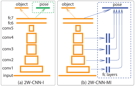
Figure 1: 2W-CNN architecture. The orange architecture is AlexNet, and we build two what/where convolutional neural network architectures from it: (a) 2W-CNN-I: object pose information (where) is linked to the top fully connected layer (fc7) only; (b) 2W-CNN-MI: object pose labels have direct pathways to all convolutional layers. The additionally appended pose architectures (green in (a) and blue in (b)) are used in training to regularize the deep feature learning process, and in testing, we prune them and use the remaining AlexNet for object recognition (what). Hence, although feedforward connection arrows are shown, all blue and green connections are only used for backpropagation.

Deep convolutional neural networks (CNNs) have achieved great success in image classification [14, 25], object detection [21, 8], image segmentation [5], activity recognition [13, 22] and many others. Typical CNN architectures, including AlexNet [14] and VGG [23], consist of several stages of convolution, activation and pooling, in which pooling subsamples feature maps, making representations locally translation invariant. After several stages of pooling, the high-level feature representations are invariant to object pose over some limited range, which is generally a desirable property. Thus, these CNNs only preserve “what” information but discard “where” or pose information through the multiple stages of pooling. However, as argued by Hinton et al. [11], artificial neural networks could use local “capsules” to encapsulate both “what” and “where” information, instead of using a single scalar to summarize the activity of a neuron. Neural architectures designed in this way have the potential to disentangle visual entities from their instantiation parameters [19, 32, 9].

In this paper, we propose a new deep architecture built on a traditional ConvNet (AlexNet, VGG), but with two label layers, one for category (what) and one for pose (where; Fig. 1). We name this a what/where convolutional neural network (2W-CNN). Here, object category is the class that an object belongs to, and pose denotes any factors causing objects from the same class to have different appearances on the images. This includes camera viewpoint, lighting, intra-class object shape variances, etc. By explicitly adding pose labels to the top of the network, 2W-CNN is forced to learn multi-level feature representations from which both object categories and pose parameters can be decoded. 2W-CNN only differs from traditional CNNs during training: two streams of error are backpropagated into the convolutional layers, one from category and the other from pose, and they jointly tune the feature filters to simultaneously capture variability in both category and pose. When training is complete, we prune all the auxiliary layers in 2W-CNN, leaving only the base architecture (traditional ConvNet, with same number of degrees of freedom as the original), and we use it to predict the category label of a new input image. By explicitly incorporating “where” information to regularize the feature learning process, we experimentally show that the learned feature representations are better delineated, resulting in better categorization accuracy.

2 Related work

This work is inspired by the concept revived by Hinton et al. [11]. They introduced “capsules” to encapsulate both “what” and “where” into a highly informative vector, and then feed both to the next layer. In their work, they directly fed translation/transformation information between input and output images as known variables into the auto-encoders, and this essentially fixes “where” and forces “what” to adapt to the fixed “where”. In contrast, in our 2W-CNN, “where” is an output variable, which is only used to back-propagate errors. It is never fed forward into other layers as known variable. In [32], the authors proposed ’stacked what-where auto-encoders’ (SWWAE), which consists of a feed-forward ConvNet (encoder), coupled with a feed-back DeConvnet (decoder). Each pooling layer from the ConvNet generates two sets of variables, “what” which records the features in the receptive field and is fed into the next layer, and “where” which remembers the position of the interesting features and is fed into the corresponding layer of the DeConvnet. Although they explicitly build “where” variables into the architecture, “where” variables are always complementary to the “what” variables and only help to record the max-pooling switch positions. In this sense, “where” is not directly involved in the learning process. In 2W-CNN, we do not have explicit “what” and “where” variables, instead, they are implicitly expressed by neurons in the intermediate layers. Moreover, “what” and “where” variables from the top output layer are jointly engaged to tune filters during learning. A recent work [9] proposes a deep generative architecture to predict video frames. The representation learned by this architecture has two components: a locally stable “what” component and a locally linear “where” component. Similar to [32], “what” and “where” variables are explicitly defined as the output of ’max-pooling’ and ’argmax-pooling’ operators, as opposed to our implicit 2W-CNN approach.

In [28], the authors propose to learn image descriptors to simultaneously recognize objects and estimate their poses. They train a linear chain feed-forward deep convolutional network by including relative pose and object category similarity and dissimilarity in their cost function, and then use the top layer output as image descriptor. However, [28] focus on learning image descriptors, then recognizing category and pose through a nearest neighbor search in descriptor space, while we investigate how explicit, absolute pose information can improve category learning. [1] introduces a method to separate manifolds from different categories while being able to predict object pose. It uses HOG features as image representations, which is known to be suboptimal compared to statistically learned deep features, while we learn deep features with the aid of pose information.

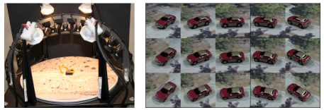
Figure 2: Left: turntable setup; Right: one exemplar car shot under different viewpoints.

In sum, our architecture differs from the above in several aspects: (1) 2W-CNN is a feed-forward discriminative architecture as opposed to an auto-encoder; (2) we do not explicitly define “what” and “where” neurons, instead, they are implicitly expressed by intermediate neurons; (3) we use explicit, absolute pose information, only during back-propagation, and not in the feed-forward pass.

Our architecture, 2W-CNN, also belongs to the framework of multi-task learning (MTL), where the basic notion is that using a single network to learn two or more related tasks yields better performance than using one dedicated network for each task [4, 2, 17]. Recently, several efforts have explored multi-task learning using deep neural networks, for face detection, phoneme recognition, scene classification and pose estimation [31, 30, 20, 12, 24]. All of them use a similar linear feed-forward architecture, with all task label layers appended onto the last fully connected layer. In the end, all tasks in these applications share the same representations. Although they [20, 31] do differentiate principal and auxiliary tasks by assigning larger/smaller weights to principal/auxiliary task losses in the objective function, they never make a distinction of tasks when designing the deep architecture. Our architecture, 2W-CNN-I (see 4.1 for definition), is similar to theirs, however, 2W-CNN-MI (see 4.1 for definition) is very different: pose is the auxiliary task, and it is designed to support the learning of the principal task (object recognition) at multiple levels. Concretely, auxiliary labels (pose) have direct pathways to all convolutional layers, such that features in the intermediate layers can be directly regularized by the auxiliary task. We experimentally show that 2W-CNN-MI, which embodies a new kind of multi-task learning, is superior to 2W-CNN-I for object recognition, and this indicates that 2W-CNN-MI is advantageous to the previously published deep multi-task learning architectures.

3 A brief introduction of the iLab-20M dataset

iLab-20M [3] was collected by hypothesizing that training can be greatly improved by using many different views of different instances of objects in a number of categories, shot in many different environments, and with pose information explicitly known. Indeed, biological systems can rely on object persistence and active vision to obtain many different views of a new physical object. In monkeys, this is believed to be exploited by the neural representation [16], though the exact mechanism remains poorly understood.

iLab-20M is a turntable dataset, with settings as follows: the turntable consists of a 14”-diameter circular plate actuated by a robotic servo mechanism. A CNC-machined semi-circular arch (radius 8.5”) holds 11 Logitech C910 USB webcams which capture color images of the objects placed on the turntable. A micro-controller system actuates the rotation servo mechanism and switches on and off 4 LED lightbulbs. Lights are controlled independently, in 5 conditions: all lights on, or one of the 4 lights on.

Objects were mainly Micro Machines toys (Galoob Corp.) and N-scale model train toys. These objects present the advantage of small scale, yet demonstrate a high level of detail and, most remarkably, a wide range of shapes (i.e., many different molds were used to create the objects, as opposed to just a few molds and many different painting schemes). Backgrounds were 125 color printouts of satellite imagery from the Internet. Every object was shot on at least 14 backgrounds, in a relevant context (e.g., cars on roads, trains on railtracks, boats on water).

In total, 1,320 images were captured for each object and background combination: 11 azimuth angles (from the 11 cameras), 8 turntable rotation angles, 5 lighting conditions, and 3 focus values (-3, 0, and +3 from the default focus value of each camera). Each image was saved with lossless PNG compression ($\sim$1 MB per image). The complete dataset hence consists of 704 object instances (15 categories), each shot on 14 or more backgrounds, with 1,320 images per object/background combination, or almost 22M images. The dataset is freely available and distributed on several hard drives. One exemplar car instance shot under different viewpoints are shown in Fig. 2(right).

4 Network Architecture and its Optimization

In this section, we introduce our new architecture, 2W-CNN, and some properties of its critical points achieved under the stochastic gradient descent (SGD) optimization.

4.1 Architecture

Our architecture, 2W-CNN, can be built on any of the CNNs, and, here, without loss of generality, we use AlexNet [14] (but see Supplementary Materials for results using VGG as well). iLab-20M has detailed pose information for each image. In the testing presented here, we only consider 10 categories, and the 8 turntable rotations and 11 camera azimuth angles, i.e., 88 discrete poses. It would be straightforward to use more categories and take light source, focus, etc. into account as well.

Our building base, AlexNet, is adapted here to be suitable for our dataset: two changes are made, compared to AlexNet in [14] (1) we change the number of units on fc6 and fc7 from 4096 to 1024, since we only have ten categories here; (2) we append a batch normalization layer after each convolution layer (see the supplementary materials for architecture specifications).

We design two variants of our approach: (1) 2W-CNN-I (with I for injection), a what/where CNN with both pose and category information injected into the top fully connected layer; (2) 2W-CNN-MI (multi-layer injection), a what/where CNN with category still injected at the top, but pose injected into the top and also directly into all 5 convolutional layers. Our motivation for multiple injection is as follows: it is generally believed that in CNNs, low- and mid-level features are learned mostly in lower layers, while, with increasing depth, more abstract high-level features are learned [29, 33]. Thus, we reasoned that detailed pose information might also be used differently by different layers. “Multi-layer injection” in 2W-CNN-MI is similar to skip connections in neural networks. Skip connection is a more generic terminology, while 2W-CNN-MI uses a specific pattern of skip connections designed specifically to make pose errors directly back propagate into lower layers. Our architecture details are as follows.

2W-CNN-I is built on AlexNet, and we further append a pose layer (88 neurons) to fc7. The architecture is shown in Fig. 1. 2W-CNN-I is trained to predict both what and where. We treat both prediction tasks as classification problems, and use softmax regression to define the individual loss. The total loss is the weighted sum of individual losses:

$$\mathcal{L}=\mathcal{L}(object)+\lambda\mathcal{L}(pose)$$ (1)

where $\lambda$ is a balancing factor, set to 1 in experiments. Although we do not have explicit what and where neurons in 2W-CNN-I, feature representations (neuron responses) at fc7 are trained such that both object category (what) and pose information (where) can be decoded; therefore, neurons in fc7 can be seen to have implicitly encoded what/where information. Similarly, neurons in intermediate layers also implicitly encapsulate what and where, since both pose and category errors at the top are back-propagated consecutively into all layers, and features learned in the low layers are adapted to both what and where.

2W-CNN-MI is built on AlexNet as well, but in this variant we add direct pathways from each convolutional layer to the pose layer, such that feature learning at each convolutional layer is directly affected by pose errors (Fig. 1). Concretely, we append two fully connected layers to each convolutional layer, including pool1, pool2, conv3 and conv4, and then add a path from the 2nd fully connected layer to the pose category layer. Fully connected layers appended to pool1 and pool2 have 512 neurons and those appended to conv3 and conv4 have 1024 neurons. At last, we directly add a pathway from fc7 to the pose label layer. The reason we do not append two additional fully connected layers to pool5 is that the original AlexNet already has fc6 and fc7 on top of pool5; thus, our fc6 and fc7 are shared by the object category layer and the pose layer.

The loss function of 2W-CNN-MI is the same as that of of 2W-CNN-I (Eq. 1). In 2W-CNN-MI, activations from 5 layers, namely pool1fc2, pool2fc2, conv3fc2, conv4fc2 and fc7, are all fed into the pose label layer, and responses at the pose layer are the accumulated activations from all 5 pathways, i.e.,

$$a(\mathscr{L}_{P})=\sum_{l}a(l)\cdot\mathcal{W}_{l-\mathscr{L}_{P}}$$ (2)

where $l$ is one from those 5 layers, $\mathcal{W}_{l-\mathscr{L}_{P}}$ is the weight matrix between $l$ and pose label layer $\mathscr{L}_{P}$, and $a(l)$ are feature activations at layer $l$.

4.2 Optimization

We use stochastic gradient descent (SGD) to minimize the loss function. In practice, it either finds a local optimum or a saddle point [6, 18] for non-convex optimization problems. How to escape a saddle point or reach a better local optimum is beyond the scope of our work here. Since both 2W-CNN and AlexNet are optimized using SGD, readers may worry that object recognition performance differences between 2W-CNN and AlexNet might be just occasional and depending on initializations, while here we show theoretically that it is easier to find a better critical point in the parameter space of 2W-CNN than in the parameter space of AlexNet by using SGD.

We prove that, in practice, a critical point of AlexNet is not a critical point of 2W-CNN, while a critical point of 2W-CNN is a critical point of AlexNet as well. Thus, if we initialize weights in a 2W-CNN from a trained AlexNet (i.e., we initialize $\omega_{1},\omega_{2}$ from the trained AlexNet, while initializing $\omega_{3}$ by random Gaussian matrices in Fig. 3), and continue training 2W-CNN by SGD, parameter solutions will gradually step away from the initial point and reach a new (better) critical point. However, if we initialize parameters in AlexNet from a trained 2W-CNN and continue training, the parameter gradients in AlexNet at the initial point are already near zero and no better critical point is found. Indeed, in the next section we verify this experimentally.

Let $\mathcal{L}=f(\omega_{1},\omega_{2})$ and $\mathcal{\hat{L}}=f(\omega_{1},\omega_{2})+g(\omega_{1},\omega_{3})$ be the softmax loss functions of AlexNet and 2W-CNN respectively, where $f(\omega_{1},\omega_{2})$ in $\mathcal{L}$ and $\mathcal{\hat{L}}$ are exactly the same, we show in practical cases that: (1) if $(\omega_{1}^{\prime},\omega_{2}^{\prime})$ is a critical point of $\mathcal{L}$, then $(\omega_{1}^{\prime},\omega_{2}^{\prime},\omega_{3})$ is not a critical point of $\mathcal{\hat{L}}$; (2) on the contrary, if $(\omega_{1}^{\prime\prime},\omega_{2}^{\prime\prime},\omega_{3}^{\prime\prime})$ is a critical point of $\hat{\mathcal{L}}$, $(\omega_{1}^{\prime\prime},\omega_{2}^{\prime\prime})$ is a critical point of $\mathcal{L}$ as well. Here we prove (1) but refer the readers to the supplementary materials for the proof of (2).

$$\left.\begin{array}[]{c}\frac{\partial\mathcal{L}}{\partial\omega_{1}^{\prime}}=\frac{\partial f}{\partial\omega_{1}^{\prime}}=\overrightarrow{0}\\ \frac{\partial\mathcal{L}}{\partial\omega_{2}^{\prime}}=\frac{\partial f}{\partial\omega_{2}^{\prime}}=\overrightarrow{0}\end{array}\right\}\rightsquigarrow\left\{\begin{array}[]{c}\frac{\partial\mathcal{\hat{L}}}{\partial\omega_{1}^{\prime}}=\frac{\partial f}{\partial\omega_{1}^{\prime}}+\frac{\partial g}{\partial\omega_{1}^{\prime}}\neq\overrightarrow{0}\\ \frac{\partial\mathcal{\hat{L}}}{\partial\omega_{2}^{\prime}}=\frac{\partial f}{\partial\omega_{2}^{\prime}}=\overrightarrow{0}\\ \frac{\partial\mathcal{\hat{L}}}{\partial\omega_{3}}=\frac{\partial g}{\partial\omega_{3}}\neq\overrightarrow{0}\end{array}\right.$$ (3)

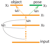
Figure 3: A simplified CNN used in proof.

Proof: assume there is at least one non-zero entry in $x_{1}\in\mbox{$\mathcal{R}$}^{1024}$ (in practice $x_{1}\neq\overrightarrow{0}$, $x_{0}\neq\overrightarrow{0}$, at least one non-zero entry, see supplementary materials), and let $x_{1}^{nz}$ be that non-zero element ($nz$ is its index, $nz\in\{1,2,...,1024\}$). Without loss of generality, we initialize all entries in $\omega_{3}\in\mathcal{R}^{88\times 1024}$ be to 0, except one entry $\omega_{3}^{nz,1}$, which is the weight between $x_{1}^{nz}$ and $x_{3}^{1}$. Since we have $x_{3}=\omega_{3}x_{1},\>(x_{3}=\mathcal{R}^{88})$, then $x_{3}^{1}=\omega_{3}^{nz,1}\cdot x_{1}^{nz}\neq 0$, while $x_{3}^{i}=0\>(i\neq 1)$.

In the case of softmax regression, we have: $\frac{\partial\mathcal{\hat{L}}}{\partial x_{3}^{c}}=1-e^{x_{3}^{c}}/\sum_{i}e^{x_{3}^{i}}$; $\frac{\partial\mathcal{\hat{L}}}{\partial x_{3}^{i}}=-e^{x_{3}^{i}}/\sum_{i}e^{x_{3}^{i}}$ when $i\neq c$, where $x_{3}^{i}$ is the $i^{th}$ entry in the vector $x_{3}$, and $c$ is the index of the ground truth pose label. Since $x_{3}^{1}\neq 0$ and $x_{3}^{i}=0(i\neq 1)$, $\frac{\partial\mathcal{\hat{L}}}{\partial x_{3}^{i}}\neq 0\>(i\in\{1,2,...,88\})$. By chain rule, we have $\frac{\partial\mathcal{\hat{L}}}{\partial\omega_{3}^{mn}}=\frac{\partial\mathcal{\hat{L}}}{\partial x_{3}^{n}}\cdot\frac{\partial x_{3}^{n}}{\partial\omega_{3}^{mn}}=\frac{\partial\mathcal{\hat{L}}}{\partial x_{3}^{n}}\cdot x_{1}^{m}$, and therefore, as long as not all entries in $x_{1}$ are 0, i.e., $x_{1}\neq\overrightarrow{0}$, we have $\frac{\partial\mathcal{\hat{L}}}{\partial\omega_{3}}=\frac{\partial\mathcal{\hat{L}}}{\partial x_{3}}\cdot x_{1}\neq\overrightarrow{0}$.

To show $\frac{\partial\mathcal{\hat{L}}}{\partial\omega_{1}^{\prime}}=\frac{\partial f}{\partial\omega_{1}^{\prime}}+\frac{\partial g}{\partial\omega_{1}^{\prime}}\neq\overrightarrow{0}$, we only have to show $\frac{\partial g}{\partial\omega_{1}^{\prime}}\neq\overrightarrow{0}$ (since $\frac{\partial f}{\partial\omega_{1}^{\prime}}=\overrightarrow{0}$). By chain rule, we have $\frac{\partial g}{\partial\omega_{1}^{\prime}}=\frac{\partial g}{\partial x_{1}}\cdot\frac{\partial x_{1}}{\partial\omega_{1}^{\prime}}$, where $\frac{\partial g}{\partial x_{1}^{i}}=0$, when $i\neq nz$; $\frac{\partial g}{\partial x_{1}^{nz}}=\omega_{3}^{nz,1}-\omega_{3}^{nz,1}\cdot e^{x_{3}^{1}}/\sum_{i}e^{x_{3}^{i}}\neq 0$. Let the weight matrix between $x_{0}$ and $x_{1}$ be $\omega_{0}^{\prime}$, and by definition, $\omega_{0}^{\prime}\in\omega_{1}^{\prime}$. Now we have $\frac{\partial x_{1}^{nz}}{\partial\omega_{0}^{\prime}}\neq\overrightarrow{0}$, otherwise $x_{0}=\overrightarrow{0}$. Therefore $\frac{\partial g}{\partial\omega_{1}^{\prime}}=\frac{\partial g}{\partial x_{1}}\cdot\frac{\partial x_{1}}{\partial\omega_{1}^{\prime}}\neq\overrightarrow{0}$, since $\frac{\partial g}{\partial x_{1}}\neq\overrightarrow{0}$ and $\frac{\partial x_{1}}{\partial\omega_{1}^{\prime}}\neq\overrightarrow{0}$.

However, a critical point of 2W-CNN is a critical point of AlexNet, i.e., Eq. 4, see supplementary materials for the proof, and next section for experimental validation.

$$\left.\begin{array}[]{c}\frac{\partial\mathcal{\hat{L}}}{\partial\omega_{1}^{\prime\prime}}=\frac{\partial f}{\partial\omega_{1}^{\prime\prime}}+\frac{\partial g}{\partial\omega_{1}^{\prime\prime}}=\overrightarrow{0}\\ \frac{\partial\mathcal{\hat{L}}}{\partial\omega_{2}^{\prime\prime}}=\frac{\partial f}{\partial\omega_{2}^{\prime\prime}}=\overrightarrow{0}\\ \frac{\partial\mathcal{\hat{L}}}{\partial\omega_{3}^{\prime\prime}}=\frac{\partial g}{\partial\omega_{3}^{\prime\prime}}=\overrightarrow{0}\end{array}\right\}\rightsquigarrow\left\{\begin{array}[]{c}\frac{\partial\mathcal{L}}{\partial\omega_{1}^{\prime\prime}}=\frac{\partial f}{\partial\omega_{1}^{\prime\prime}}=\overrightarrow{0}\\ \frac{\partial\mathcal{L}}{\partial\omega_{2}^{\prime\prime}}=\frac{\partial f}{\partial\omega_{2}^{\prime\prime}}=\overrightarrow{0}\end{array}\right.$$ (4)

5 Experiments

In experiments, we demonstrate the effectiveness of 2W-CNN for object recognition against linear-chain deep architectures (e.g., AlexNet) using the iLab-20M dataset. We do both quantitative comparisons and qualitative evaluations. Further more, to show the learned features on iLab-20M are useful for generic object recognitions, we adop the “pretrain - fine-tuning” paradigm, and fine tune object recognition on the ImageNet dataset [7] using the pretrained AlexNet and 2W-CNN-MI features on the iLab-20M dataset.

5.1 Dataset setup

Object categories: we use 10 (out of 15) categories of objects in our experiments (Fig. 6), and, within each category, we randomly use 3/4 instances as training data, and the remaining 1/4 instances for testing. Under this partition, instances in test are never seen during training, which minimizes the overlap between training and testing.

Pose: here we take images shot under one fixed light source (with all 4 lights on) and camera focus (focus = 1), but all 11 camera azimuths and all 8 turntable rotations (88 poses).

We end up with 0.65M (654,929) images in the training set and 0.22M (217,877) in the test set. Each image is associated with 1 (out of 10) object category label and 1 (out of 88) pose label.

5.2 CNNs setup

We train 3 CNNs, AlexNet, 2W-CNN-I and 2W-CNN-MI, and compare their performances on object recognition. We use the same initialization for their common parameters: we first initialize AlexNet with random Gaussian weights, and re-use these weights to initialize the AlexNet component in 2W-CNN-I and 2W-CNN-MI. We then randomly initialize the additional parameters in 2W-CNN-I / 2W-CNN-MI.

No data augmentation: to train AlexNet for object recognition, in practice, one often takes random crops and also horizontally flips each image to augment the training set. However, to train 2W-CNN-I and 2W-CNN-MI, we could take random crops but we should not horizontally flip images, since flipping creates a new unknown pose. For a fair comparison, we do not augment the training set, such that all 3 CNNs use the same amounts of images for training.

Optimization settings: we run SGD to minimize the loss function, but use different starting learning and dropout rates for different CNNs. AlexNet and 2W-CNN-I have similar amounts of parameters, while 2W-CNN-MI has 15 times more parameters during training (but remember that all three models have the exact same number of parameters during test). To control overfitting, we use a smaller starting learning rate (0.001) and a higher dropout rate (0.7) for 2W-CNN-MI, while for AlexNet and 2W-CNN-I, we set the starting learning rate and dropout rate to be 0.01 and 0.5. Each network is trained for 30 epochs, and approximately 150,000 iterations. To further avoid any training setup differences, within each training epoch, we fix the image order. We train CNNs using the publicly available Matconvnet [27] toolkit on a Nvidia Tesla K40 GPU.

5.3 Performance evaluation

In this section, we evaluate object recognition performance of the 3 CNNs. As mentioned, for both 2W-CNN-I and 2W-CNN-MI, object pose information is only used in training, but the associated machinery is pruned away before test (Fig. 1).

Since all three architectures are trained by SGD, the solutions depend on initializations. To alleviate the randomness of SGD, we run SGD under different initializations and report the mean accuracy. We repeat the training of 3 CNNs under 5 different initializations, and report their mean accuracies and standard deviations in Table 1. Our main result is: (1) 2W-CNN-MI and 2W-CNN-I outperform AlexNet by $6\%$ and $5\%$; (2) 2W-CNN-MI further improves the accuracy by $1\%$ compared with 2W-CNN-I. This shows that, under the regularization of additional pose information, 2W-CNN learns better deep features for object recognition.

	AlexNet	2W-CNN-I	2W-CNN-MI
accuracy	0.785 ($\pm$0.0019)	0.837 ($\pm$0.0022)	0.848 ($\pm$0.0031)
mAP	0.787	0.833	0.850

Table 1: Object recognition performances of AlexNet, 2W-CNN-I and 2W-CNN-MI on iLab-20M dataset. 2W-CNN-MI performed significantly better than AlexNet (t-test, $p<1.6\cdot 10^{-5}$), and 2W-CNN-I ($p<6.3\cdot 10^{-5}$) as well. 2W-CNN-MI was also significantly better than 2W-CNN-I ($p<.013$).

As proven in Sec. 4.2, in practice a critical point of AlexNet is not a critical point of 2W-CNN, while a critical point of 2W-CNN is a critical point of AlexNet. We verify critical points of two networks using experiments: (1) we use the trained AlexNet parameters to initialize 2W-CNN, and run SGD to continue training 2W-CNN; (2) conversely, we initialize AlexNet from the trained 2W-CNN and continue training for some epochs. We plot the object recognition error rates on test data against training epochs in Fig. 4. As shown, 2W-CNN obviously reaches a new and better critical point distinct from the initialization, while AlexNet stays around the same error rate as the initialization.

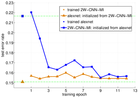
Figure 4: Critical points of CNNs. We initialize one network from the trained other network, continue training, and record test errors after each epoch. Starting from a critical point of AlexNet, 2W-CNN-MI steps away from it and reaches a new and better critical point, while AlexNet initialized from 2W-CNN-MI fails to further improve on test performance.

5.4 Decoupling of what and where

2W-CNNs are trained to predict what and where. Although 2W-CNNs do not have explicit what and where neurons, we experimentally show that what and where information is implicitly expressed by neurons in different layers.

One might speculate that in 2W-CNN, more than in standard AlexNet, different units in the same layer might become either pose-defining or identity-defining. A pose-defining unit should be sensitive to pose, but invariant to object identity, and conversely. To quantify this, we use entropy to measure the uncertainty of each unit to pose and identity. We estimate pose and identity entropies of each unit as follows: we use all test images as inputs, and we calculate the activation ($a_{i}$) of each image for that unit. Then we compute histogram distributions of activations against object category (10 categories in our case) and pose (88 poses), and let two distributions be $\mathcal{P}_{obj}$ and $\mathcal{P}_{pos}$ respectively. The entropies of these two distributions, $\mathscr{E}(\mathcal{P}_{obj})$ and $\mathscr{E}(\mathcal{P}_{pos})$, are defined to be the object and pose uncertainty of that unit. For units to be pose-defining or identity-defining, one entropy should be low and the other high, while for units with identity and pose coupled together, both entropies are high.

Assume there are $n$ units on some layer $l$ (e.g., 256 units on pool5), each with identity and pose entropy $\mathscr{E}^{i}(obj)$ and $\mathscr{E}^{i}(pos)$ ($i\in\{1,2,...,n\}$), and we organize $n$ identity entropies into a vector $\mathscr{E}(obj)=[\mbox{$\mathscr{E}$}^{1}(obj),\mbox{$\mathscr{E}$}^{2}(obj),...,\mbox{$\mathscr{E}$}^{n}(obj)]$ and $n$ pose entropies into a vector $\mathscr{E}(pos)=[\mbox{$\mathscr{E}$}^{1}(pos),\mbox{$\mathscr{E}$}^{2}(pos),...,\mbox{$\mathscr{E}$}^{n}(pos)]$. If $n$ units are pose/identity decoupled, then $\mathscr{E}(obj)$ and $\mathscr{E}(pos)$ are expected to be negatively correlated. Concretely, for entries at their corresponding locations, if one is large, the other is desirable to be small. We define the correlation coefficient in Eq. 5 between $\mathscr{E}(obj)$ and $\mathscr{E}(pos)$ to be the decouple-ness of $n$ units on the layer $l$, more negative it is, the better units are pose/identity decoupled.

$$\gamma=corrcoef\,(\mathscr{E}(obj),\mathscr{E}(pose))$$ (5)

We compare the decouple-ness of units from our 2W-CNN architecture against those from AlexNet. We take all units from the same layer, including pool1, pool2, conv3, conv4, pool5, fc6 and fc7, compute their decouple-ness and plot them in Fig. 5. It reveals: (1) units in 2W-CNN from different layers have been better what/where decoupled, some are learned to capture pose, while others are learned to capture identity; (2) units in the earlier layers (e.g., pool2, conv3, conv4) are better decoupled in 2W-CNN-MI than in 2W-CNN-I, which is expected since pose errors are directly back-propagated into these earlier layers in 2W-CNN-MI. This indicates as well pose and identity information are implicitly expressed by different units, although we have no explicit what/where neurons in 2W-CNN.

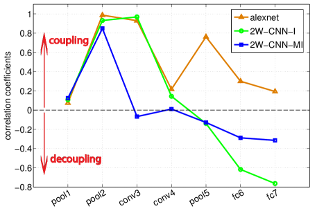
Figure 5: Decoupling of what and where. This figure shows the pose/identity decouple-ness of units from the same layer. 2W-CNN makes pose and identity better decoupled than AlexNet, which indicates neurons at intermediate layers of 2W-CNN implicitly segregate what and where information.

5.5 Feature visualizations

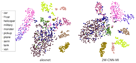
Figure 6: t-SNE visualization of fc7 features. The learned deep features at fc7 are better delineated by 2W-CNN than AlexNet.

We extract 1024-dimensional features from fc7 of 2W-CNN and AlexNet as image representations, and use t-SNE [26] to compute their 2D embeddings and plot results in Fig. 6. Seen qualitatively, object categories are better separated by 2W-CNN representations: For example, “military car” (magenta pentagram) and “tank” (purple pentagram) representations under 2W-CNN have a clear boundary, while their AlexNet representation distributions penetrate into each other. Similarly, “van” (green circle) and “car” (brown square) are better delineated by 2W-CNN as well.

We further visualize receptive fields of units at different layers of AlexNet and 2W-CNN. The filters of conv1 can be directly visualized, while to visualize RFs of units on other layers, we adopt methods used in [33]: we use all test images as input, compute their activation responses of each unit on each layer, and average the top 100 images with the strongest activations as a receptive field visualization of each unit. Fig. 7 shows the receptive fields of units on conv1, poo2, conv3 and pool5 of two architectures, AlexNet on top and 2W-CNN-MI on bottom. It suggests qualitatively that: (1) 2W-CNN has more distinctive and fewer dead filters on conv1; (2) AlexNet learns many color filters, which can be seen especially from conv1, pool2 and conv3. While color benefits object recognition in some cases, configural and structural information is more desirable in most cases. 2W-CNN learns more structural filters.

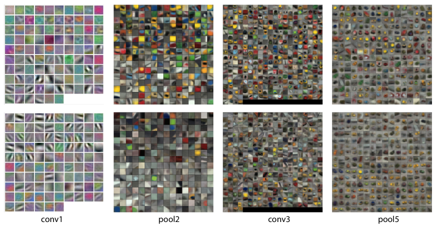
Figure 7: Visualization of receptive fields of units at different layers. The top (bottom) row shows receptive fields of AlexNet (2W-CNN).

5.6 Extension to ImageNet object recognition

ImageNet has millions of labeled images, and thus pre-training a ConvNet on another dataset has been shown to yield insignificant effects [10, 15]. To show that the pretrained 2W-CNN-MI and AlexNet on iLab-20M learns useful features for generic object recognition, we fine-tune the learned weights on ImageNet when we can only access a small amount of labeled images. We fine-tune AlexNet using 5, 10, 20, 40 images per class from the ILSVRC-2010 challenge. AlexNet is trained and evaluated on ImageNet under three cases: (1) from scratch (use random Gaussian initialization), (2) from pretrained AlexNet on iLab-20M, (3) from pretrained 2W-CNN-MI on iLab-20M. When we pretrain 2W-CNN-MI on the iLab-20M dataset, we set the units on fc6 and fc7 back to 4096. AlexNet used in pretraining and finetuning follows exactly as the one in [14]. We report top-5 object recognition accuracies in Table 2.

# of images/class	5	10	20	40
AlexNet (scratch)	1.47	4.15	16.45	25.89
AlexNet (AlexNet-iLab20M)	7.74	12.54	19.42	28.75
AlexNet (2W-CNN-MI-iLab20M)	9.27	14.85	23.14	31.60

Table 2: Top-5 object recognition accuracies ($\%$) on the test set of ILSVRC-2010, with 150 images per class and a total of 150K test images. First, fine-tuning AlexNet from the pretrained features on the iLab-20M dataset clearly outperforms training AlexNet from scratch, which shows features learned on the iLab-20M dataset generalizes to ImageNet as well. Second, fine-tuning from the pretrained 2W-CNN-MI (2W-CNN-MI-iLab20M) performs even better than from the pretrained AlexNet (AlexNet-iLab20M), which shows our 2W-CNN-MI architecture learns even more effective features for object recognition than AlexNet.

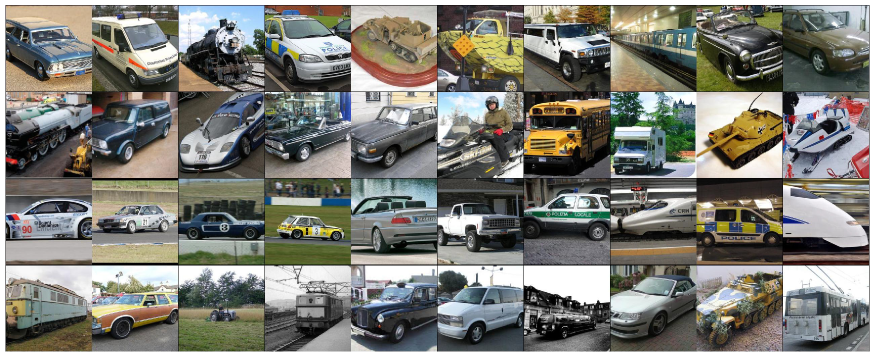
Figure 8: Pose estimation of ImageNet images using trained 2W-CNN-MI on the iLab-20M dataset. Given a test image, 2W-CNN-Mi trained on the iLab-20M dataset could predict one discrete pose (out of 88). In the figure, each row shows the top 10 vehicle images which have the same predicted pose label. Qualitatively, images on the same row do have similar view points, showing 2W-CNN-MI generalizes well to natural images, even though it is trained on our turntable dataset.

Quantitative results: we have two key observations (1) when a limited number of labeled images is available, fine-tuning AlexNet from the pretrained features on the iLab-20M dataset outperforms training AlexNet from scratch, e.g., the relative improvement is as large as $\sim 530\%$ when we have only 5 samples per class, when more labeled images are available, the improvement decreases, but we still achieve $\sim 22\%$ improvements when 40 labeled images per class are used. This clearly shows features learned on the iLab-20M dataset generalize well to the natural image dataset ImageNet. (2) fine-tuning from the pretrained 2W-CNN-MI on iLab-20M performs even better than from the pretrained AlexNet on iLab-20M, and this shows that 2W-CNN-MI learns even better features for general object recognition than AlexNet. These empirical results show that training object categories jointly with pose information makes the learned features more effective.

Qualitative results: the trained 2W-CNN-MI on iLab-20M could predict object pose as well; here, we directly use the trained 2W-CNN-MI to predict pose for each test image from ILSVRC-2010. Each test image is assigned a pose label (one out of 88 discrete poses, in our case) with some probability. For each discrete pose, we choose 10 vehicles, whose prediction probabilities at that pose are among the top 10, and visualize them in Fig. 8. Each row in Fig. 8 shows top 10 vehicles whose predicted pose label are the same, and as observed, they do have very similar camera viewpoints. This qualitative result shows pose features learned by 2W-CNN-MI generalize to ImageNet as well.

6 Conclusion

Although in experiments we built 2W-CNN on AlexNet, we could use any feed-forward architecture as a base. Our results show that better training can be achieved when explicit absolute pose information is available. We further show that the pretrained AlexNet and 2W-CNN features on iLab-20M generalizes to the natural image dataset ImageNet, and moreover, the pretrained 2W-CNN features are shown to be advantageous to the pretrained AlexNet features in real dataset as well. We believe that this is an important finding when designing new datasets to assist training of object recognition algorithms, in complement with the existing large test datasets and challenges.

Acknowledgement: This work was supported by the National Science Foundation (grant numbers CCF-1317433 and CNS-1545089), the Army Research Office (W911NF- 12-1-0433), and the Office of Naval Research (N00014-13- 1-0563). The authors affirm that the views expressed herein are solely their own, and do not represent the views of the United States government or any agency thereof.

References

- [1] A. Bakry and A. Elgammal. Untangling object-view manifold for multiview recognition and pose estimation. In Computer Vision–ECCV 2014, pages 434–449. Springer, 2014.
- [2] J. Baxter. A model of inductive bias learning. J. Artif. Intell. Res.(JAIR), 12:149–198, 2000.
- [3] A. Borji, S. Izadi, and L. Itti. ilab-20m: A large-scale controlled object dataset to investigate deep learning. In The IEEE Conference on Computer Vision and Pattern Recognition (CVPR), June 2016.
- [4] R. Caruana. Multitask learning. Machine learning, 28(1):41–75, 1997.
- [5] L.-C. Chen, G. Papandreou, I. Kokkinos, K. Murphy, and A. L. Yuille. Semantic image segmentation with deep convolutional nets and fully connected crfs. arXiv preprint arXiv:1412.7062, 2014.
- [6] Y. N. Dauphin, R. Pascanu, C. Gulcehre, K. Cho, S. Ganguli, and Y. Bengio. Identifying and attacking the saddle point problem in high-dimensional non-convex optimization. In Advances in Neural Information Processing Systems, pages 2933–2941, 2014.
- [7] J. Deng, W. Dong, R. Socher, L.-J. Li, K. Li, and L. Fei-Fei. Imagenet: A large-scale hierarchical image database. In Computer Vision and Pattern Recognition, 2009. CVPR 2009. IEEE Conference on, pages 248–255. IEEE, 2009.
- [8] R. Girshick, J. Donahue, T. Darrell, and J. Malik. Rich feature hierarchies for accurate object detection and semantic segmentation. In Computer Vision and Pattern Recognition (CVPR), 2014 IEEE Conference on, pages 580–587. IEEE, 2014.
- [9] R. Goroshin, M. Mathieu, and Y. LeCun. Learning to linearize under uncertainty. arXiv preprint arXiv:1506.03011, 2015.
- [10] G. Hinton, L. Deng, D. Yu, G. E. Dahl, A.-r. Mohamed, N. Jaitly, A. Senior, V. Vanhoucke, P. Nguyen, T. N. Sainath, et al. Deep neural networks for acoustic modeling in speech recognition: The shared views of four research groups. Signal Processing Magazine, IEEE, 29(6):82–97, 2012.
- [11] G. E. Hinton, A. Krizhevsky, and S. D. Wang. Transforming auto-encoders. In Artificial Neural Networks and Machine Learning–ICANN 2011, pages 44–51. Springer, 2011.
- [12] Y. Huang, W. Wang, L. Wang, and T. Tan. Multi-task deep neural network for multi-label learning. In Image Processing (ICIP), 2013 20th IEEE International Conference on, pages 2897–2900. IEEE, 2013.
- [13] A. Karpathy, G. Toderici, S. Shetty, T. Leung, R. Sukthankar, and L. Fei-Fei. Large-scale video classification with convolutional neural networks. In Computer Vision and Pattern Recognition (CVPR), 2014 IEEE Conference on, pages 1725–1732. IEEE, 2014.
- [14] A. Krizhevsky, I. Sutskever, and G. E. Hinton. Imagenet classification with deep convolutional neural networks. In Advances in neural information processing systems, pages 1097–1105, 2012.
- [15] Y. LeCun, Y. Bengio, and G. Hinton. Deep learning. Nature, 521(7553):436–444, 2015.
- [16] N. Li and J. J. DiCarlo. Unsupervised natural visual experience rapidly reshapes size-invariant object representation in inferior temporal cortex. Neuron, 67(6):1062–1075, 2010.
- [17] S. J. Pan and Q. Yang. A survey on transfer learning. Knowledge and Data Engineering, IEEE Transactions on, 22(10):1345–1359, 2010.
- [18] R. Pascanu, Y. N. Dauphin, S. Ganguli, and Y. Bengio. On the saddle point problem for non-convex optimization. arXiv preprint arXiv:1405.4604, 2014.
- [19] M. A. Ranzato, F. J. Huang, Y.-L. Boureau, and Y. LeCun. Unsupervised learning of invariant feature hierarchies with applications to object recognition. In Computer Vision and Pattern Recognition, 2007. CVPR’07. IEEE Conference on, pages 1–8. IEEE, 2007.
- [20] M. L. Seltzer and J. Droppo. Multi-task learning in deep neural networks for improved phoneme recognition. In Acoustics, Speech and Signal Processing (ICASSP), 2013 IEEE International Conference on, pages 6965–6969. IEEE, 2013.
- [21] P. Sermanet, D. Eigen, X. Zhang, M. Mathieu, R. Fergus, and Y. LeCun. Overfeat: Integrated recognition, localization and detection using convolutional networks. arXiv preprint arXiv:1312.6229, 2013.
- [22] K. Simonyan and A. Zisserman. Two-stream convolutional networks for action recognition in videos. In Advances in Neural Information Processing Systems, pages 568–576, 2014.
- [23] K. Simonyan and A. Zisserman. Very deep convolutional networks for large-scale image recognition. CoRR, abs/1409.1556, 2014.
- [24] H. Su, C. R. Qi, Y. Li, and L. J. Guibas. Render for cnn: Viewpoint estimation in images using cnns trained with rendered 3d model views. In Proceedings of the IEEE International Conference on Computer Vision, pages 2686–2694, 2015.
- [25] C. Szegedy, W. Liu, Y. Jia, P. Sermanet, S. Reed, D. Anguelov, D. Erhan, V. Vanhoucke, and A. Rabinovich. Going deeper with convolutions. arXiv preprint arXiv:1409.4842, 2014.
- [26] L. Van der Maaten and G. Hinton. Visualizing data using t-sne. Journal of Machine Learning Research, 9(2579-2605):85, 2008.
- [27] A. Vedaldi and K. Lenc. Matconvnet – convolutional neural networks for matlab.
- [28] P. Wohlhart and V. Lepetit. Learning descriptors for object recognition and 3d pose estimation. arXiv preprint arXiv:1502.05908, 2015.
- [29] M. D. Zeiler and R. Fergus. Visualizing and understanding convolutional networks. In Computer Vision–ECCV 2014, pages 818–833. Springer, 2014.
- [30] C. Zhang and Z. Zhang. Improving multiview face detection with multi-task deep convolutional neural networks. In Applications of Computer Vision (WACV), 2014 IEEE Winter Conference on, pages 1036–1041. IEEE, 2014.
- [31] Z. Zhang, P. Luo, C. C. Loy, and X. Tang. Facial landmark detection by deep multi-task learning. In Computer Vision–ECCV 2014, pages 94–108. Springer, 2014.
- [32] J. Zhao, M. Mathieu, R. Goroshin, and Y. Lecun. Stacked what-where auto-encoders. arXiv preprint arXiv:1506.02351, 2015.
- [33] B. Zhou, A. Khosla, A. Lapedriza, A. Oliva, and A. Torralba. Object detectors emerge in deep scene cnns. arXiv preprint arXiv:1412.6856, 2014.