Weak Unique Continuation Property and a Related Inverse Source Problem for Time-Fractional Diffusion-Advection Equations

Abstract

In this paper, we first establish a weak unique continuation property for time-fractional diffusion-advection equations. The proof is mainly based on the Laplace transform and the unique continuation properties for elliptic and parabolic equations. The result is weaker than its parabolic counterpart in the sense that we additionally impose the homogeneous boundary condition. As a direct application, we prove the uniqueness for an inverse problem on determining the spatial component in the source term in by interior measurements. Numerically, we reformulate our inverse source problem as an optimization problem, and propose an iteration thresholding algorithm. Finally, several numerical experiments are presented to show the accuracy and efficiency of the algorithm.

Keywords

fractional diffusion equation, weak unique continuation, inverse source problem, iterative thresholding algorithm

AMS Subject Classifications 35R11, 26A33, 35R30

sectionIntroduction

2.3ex plus.2ex

Let $\Omega\subset\mathbb{R}^{d}$ be an open bounded domain with a sufficiently smooth boundary (e.g., of $C^{2}$-class) and $T>0$. Let $m\in\{1,2,\ldots\}$ and $\alpha_{j},q_{j}$ ($j=1,2,\ldots,m$) be positive constants such that $1>\alpha_{1}>\alpha_{2}>\cdots>\alpha_{m}>0$. By $\partial_{t}^{\alpha_{j}}$ we denote the Caputo derivative (see, e.g., [26, §2.4.1])

$$\partial_{t}^{\alpha_{j}}g(t):=\frac{1}{\Gamma(1-\alpha_{j})}\int_{0}^{t}\frac{g^{\prime}(\tau)}{(t-\tau)^{\alpha_{j}}}\,\mathrm{d}\tau,$$

where $\Gamma(\,\cdot\,)$ stands for the Gamma function. For $(x,t)\in Q:=\Omega\times(0,T)$, we define the operator

$$\mathcal{P}u(x,t):=\sum_{j=1}^{m}q_{j}\partial_{t}^{\alpha_{j}}u(x,t)+\mathcal{A}u(x,t)+B(x)\cdot\nabla u(x,t).$$ (1.1)

Here $\mathcal{A}$ is a symmetric second-order elliptic operator which will be defined at the beginning of Section Weak Unique Continuation Property and a Related Inverse Source Problem for Time-Fractional Diffusion-Advection Equations, and $B(x)=(b_{1}(x),b_{2}(x),\ldots,b_{d}(x))$. Without loss of generality, we set $q_{1}=1$. In this paper, we investigate the following initial-boundary value problem for the time-fractional diffusion-advection equation

$$\begin{cases}\mathcal{P}u=F&\mbox{in }Q,\\ u=a&\mbox{in }\Omega\times\{0\},\\ u=0\mbox{ or }\partial_{\mathcal{A}}u=0&\mbox{on }\partial\Omega\times(0,T),\end{cases}$$ (1.2)

where $\partial_{\mathcal{A}}u$ denotes the normal derivative associated with the elliptic operator $\mathcal{A}$. The conditions on the initial data $a$, the source term $F$, coefficients involved in $\mathcal{P}$ and the definitions of $\partial_{\mathcal{A}}$ will be specified later in Section Weak Unique Continuation Property and a Related Inverse Source Problem for Time-Fractional Diffusion-Advection Equations.

In various forms and generalities, the time-fractional parabolic operator $\mathcal{P}$ in (1.1) has gained increasing popularity among mathematicians within the last few decades, owing to its applicability in describing the anomalous diffusion phenomena in highly heterogeneous media (see [1, 9] and the references therein). The fundamental theory for the single-term (i.e., $m=1$) case of (1.1) was established around the early 2010s, represented by the maximum principle proved in Luchko [22] and the well-posedness, analyticity and asymptotic behavior proved in Sakamoto and Yamamoto [27]. Thereafter, most of the properties were parallelly generalized to the multi-term case (i.e., $m>1$) in [23, 12, 13], and especially the maximum principle was recently improved to stronger ones in [21, 19]. Meanwhile, corresponding numerical methods have also been well-developed and we refer e.g.​ to [11, 10]. In contrast to the usual parabolic equations characterized by the exponential decay in time and Gaussian profile in space, it reveals that the fractional diffusion equations driven by $\mathcal{P}$ possess properties of slow decay in time and long-tailed profile in space. Nevertheless, we notice that most of the existing literature only treated the symmetric elliptic operator (i.e., $B\equiv 0$ in (1.1)), in which the existence of eigensystem provides convenience for the argument.

Other than the above mentioned aspects, the unique continuation property is also one of the remarkable characterizations of parabolic equations, which asserts the vanishment of a solution to a homogeneous problem in an open subset implies its vanishment in the whole domain (see, e.g., [29]). The unique continuation property is not only important by itself, but also significant in its applications to many related control and inverse problems. However, the publications on its generalization to fractional diffusion equations are rather limited to the best of the authors’ knowledge. For the special half-order fractional diffusion equation (i.e., $m=1$, $\alpha_{1}=\frac{1}{2}$ and $\mathcal{A}=-\triangle$ in (1.1)), the unique continuation property was proved in Xu, Cheng and Yamamoto [31] for $d=1$ and Cheng, Lin and Nakamura [4] for $d=2$ via Carleman estimates for the operator $\partial_{t}-\triangle^{2}$. For a general fractional order in the $(0,1)$ interval, Lin and Nakamura [17] recently obtained a unique continuation property by using a newly established Carleman estimate based on calculus of pseudo-differential operators. We notice that the conclusion in [17] requires the homogeneous initial condition, which possibly roots in the memory effect of time-fractional diffusion equations.

Regarding the unique continuation property, the first focus of this paper is the investigation of the following problem.

Problem 1.1

Let $u$ be the solution of (1.2), where the source term $F=0$. Then does $u=0$ in some open subset of $Q=\Omega\times(0,T)$ implies $u\equiv 0$ in $Q$ under certain conditions?

In Theorem 2.5, we will give an affirmative answer to this problem. Compared with the existing literature, we formulate the problem on the more general time-fractional parabolic operator $\mathcal{P}$ with non-symmetric elliptic part in space. Meanwhile, we allow non-vanishing initial data at the cost of the homogeneous Dirichlet or Neumann boundary condition.

On the other hand, parallelly with the intensive attention paid to forward problems for time-fractional diffusion equations, there are also rapidly growing publications on the related inverse problems with various combinations of unknown functions and observation data. Here we do not intend to give a full list of bibliographies, but just mention [5, 16, 24, 33, 15, 14] and the references therein for readers’ curiosity. Nevertheless, it turns out that the majority of them concentrate on coefficient inverse problems. In contrast, the study on inverse source problems is far from satisfactory and mainly restricts to several special cases due to the lack of specified techniques. In the one-dimensional case, Zhang and Xu [34] proved the uniqueness for determining a time-independent source term by the partial boundary data, and a conditional stability for the recovery of the spatial component in the source term was proved for the half-order case in Yamamoto and Zhang [32]. With the final overdetermining data, Sakamoto and Yamamoto [28] showed the generic well-posedness for reconstructing the spatial component. Similarly to the situation of the forward problems reviewed above, it reveals that almost all papers treating the related inverse problems also rely heavily on the symmetry of the involved elliptic operator, regardless of the practical importance of the non-symmetric case.

Keeping the above points in mind, we are also interested in studying the following inverse source problem, which is the second focus of this paper.

Problem 1.2

Let $u$ be the solution of (1.2), where the initial data $a=0$ and the source term takes the form of separated variables, namely $F(x,t)=f(x)\,\mu(t)$. Provided that the temporal component $\mu(t)$ $(0\leq t\leq T)$ is known, can we uniquely determine the spatial component $f(x)$ $(x\in\Omega)$ by the partial interior observation of $u$ in some open subset of $Q=\Omega\times(0,T)$ under certain conditions?

Theorem 2.6 answers this problem affirmatively. Obviously, the above problem is closely related to Problem 1.1 in the sense that both are concerned with the partial interior information of the solution. Practically, the formulation of Problem 1.2 is applicable in the determination of the space distribution $f$ modeling the contaminant source, where the anomalous diffusion phenomena is described by (1.2) and the time evolution $\mu$ of the contaminant is known in advance. As far as the authors know, the above problem has not yet been considered in form of the generalized time-fractional parabolic operator $\mathcal{P}$.

By restricting the open subset in Problems 1.1–1.2 as a cylindrical subdomain, first we will give an affirmative answer to Problem 1.1 in two cases, that is, either the multi-term fractional diffusion equation without an advection term or the single-term one with an advection term. The statement concluded in Theorem 2.5 will be called as the weak unique continuation property because we impose the homogeneous Dirichlet or Neumann boundary condition, which is absent in the usual parabolic prototype. As a direct application, the uniqueness for Problem 1.2 can be immediately proved with the aid of a fractional version of Duhamel’s principle. For the numerical reconstruction, we reformulate Problem 1.2 as an optimization problem with Tikhonov regularization. After the derivation of the corresponding variational equation, we can characterize the minimizer by employing the associated backward fractional diffusion equation, which results in an efficient iterative method.

The remainder of this paper is organized as follows. Preparing all necessities about the weak solution of (1.2), in Section Weak Unique Continuation Property and a Related Inverse Source Problem for Time-Fractional Diffusion-Advection Equations we state the main results answering Problems 1.1 and 1.2 in Theorems 2.5 and 2.6, respectively. Then Section Weak Unique Continuation Property and a Related Inverse Source Problem for Time-Fractional Diffusion-Advection Equations is devoted to the proofs of the above theorems. In Section Weak Unique Continuation Property and a Related Inverse Source Problem for Time-Fractional Diffusion-Advection Equations, we propose the iterative thresholding algorithm for the numerical treatment of our inverse source problem, followed by several numerical examples illustrating the performance of the proposed method in Section Weak Unique Continuation Property and a Related Inverse Source Problem for Time-Fractional Diffusion-Advection Equations. As technical details, we provide the proofs for the well-posedness of the weak solutions of (1.2) in Appendix Weak Unique Continuation Property and a Related Inverse Source Problem for Time-Fractional Diffusion-Advection Equations.

sectionPreliminaries and Main Results

2.3ex plus.2ex

In this section, we first set up notations and terminologies, and review some of standard facts on the fractional calculus. Let $L^{2}(\Omega)$ be a usual $L^{2}$-space with the inner product $(\,\cdot\,,\,\cdot\,)$ and $H_{0}^{1}(\Omega)$, $H^{2}(\Omega)$, etc.​ denote the usual Sobolev spaces. Especially, for $\beta\in(0,1)$ we define the fractional Sobolev space $H^{\beta}(0,T)$ in time (see Adams [2]). The elliptic operator $\mathcal{A}$ is defined for $\psi\in\mathcal{D}(\mathcal{A}):=\{\psi\in H^{2}(\Omega);\,\psi=0\mbox{ on }\partial\Omega\}$ or $\{\psi\in H^{2}(\Omega);\,\partial_{\mathcal{A}}\psi=0\mbox{ on }\partial\Omega\}$ as

$$\mathcal{A}\psi(x):=-\sum_{i,j=1}^{d}\partial_{j}(a_{ij}(x)\partial_{i}\psi(x))+c(x)\psi(x),$$

where $\partial_{\mathcal{A}}\psi(x):=\sum_{i,j=1}^{d}a_{ij}(x)\nu_{i}(x)\partial_{j}\psi(x)$ and $\nu(x)=(\nu_{1}(x),\ldots,\nu_{d}(x))$ denotes the outward unit normal vector to $\partial\Omega$ at $x\in\partial\Omega$. Here we assume $a_{ij}=a_{ji}\in C^{1}(\overline{\Omega})$ ($1\leq i,j\leq d$), $c\in L^{\infty}(\Omega)$ and there exists a constant $\kappa>0$ such that

$$\sum_{i,j=1}^{d}a_{ij}(x)\xi_{i}\xi_{j}\geq\kappa\sum_{i=1}^{d}\xi_{i}^{2},\quad\forall\,x\in\overline{\Omega},\ \forall\,(\xi_{1},\ldots,\xi_{d})\in\mathbb{R}^{d}.$$

When the zeroth order coefficient $c\geq 0$ in $\Omega$, we introduce the eigensystem $\{(\lambda_{n},\varphi_{n})\}_{n=1}^{\infty}$ of $\mathcal{A}$ such that $0\leq\lambda_{1}<\lambda_{2}\leq\cdots$, $\lambda_{n}\to\infty$ ($n\to\infty$) and $\{\varphi_{n}\}\subset\mathcal{D}(\mathcal{A})$ forms a complete orthonormal basis of $L^{2}(\Omega)$. Considering the possibility of $\lambda_{1}=0$, we define $\widetilde{\mathcal{A}}:=\mathcal{A}+1$. Then the corresponding eigenvalues $\widetilde{\lambda}_{n}:=\lambda_{n}+1$ are all strictly positive, and the fractional power $\widetilde{\mathcal{A}}^{\gamma}$ is defined for $\gamma\in\mathbb{R}$ (e.g., [25]) as

$$\widetilde{\mathcal{A}}^{\gamma}\psi=\sum_{n=1}^{\infty}\widetilde{\lambda}_{n}^{\gamma}(\psi,\varphi_{n})\varphi_{n},$$

where

$$\psi\in\mathcal{D}(\widetilde{\mathcal{A}}^{\gamma}):=\left\{\psi\in L^{2}(\Omega);\sum_{n=1}^{\infty}\widetilde{\lambda}_{n}^{2\gamma}|(\psi,\varphi_{n})|^{2}<\infty\right\}$$

and $\mathcal{D}(\widetilde{\mathcal{A}}^{\gamma})$ is a Hilbert space with the norm

$$\|\psi\|_{\mathcal{D}(\widetilde{\mathcal{A}}^{\gamma})}=\left(\sum_{n=1}^{\infty}\left|\widetilde{\lambda}_{n}^{\gamma}(\psi,\varphi_{n})\right|^{2}\right)^{1/2}.$$

On the other hand, the first order coefficient $B=(b_{1},\ldots,b_{d})$ in the operator $\mathcal{P}$ is assumed to be in $(L^{\infty}(\Omega))^{d}$.

By $J_{0+}^{\alpha}$ we denote the Riemann-Liouville integral operator, which is defined by

$$J_{0+}^{\alpha}g(t):=\frac{1}{\Gamma(\alpha)}\int_{0}^{t}\frac{g(\tau)}{(t-\tau)^{1-\alpha}}\,\mathrm{d}\tau,\quad\alpha>0.$$

Then the Caputo derivative $\partial_{t}^{\alpha}$ can be rephrased as $\partial_{t}^{\alpha}g(t)=J_{0+}^{1-\alpha}\frac{\mathrm{d}}{\mathrm{d}t}g(t)$. Parallelly, we define the backward Riemann-Liouville integral operator $J^{\alpha}_{T-}$ by

$$J^{\alpha}_{T-}g(t)=\frac{1}{\Gamma(\alpha)}\int_{t}^{T}\frac{g(\tau)}{(\tau-t)^{1-\alpha}}\,\mathrm{d}\tau,$$

and the backward Riemann-Liouville fractional derivative by $D_{t}^{\alpha}g(t):=-\frac{\mathrm{d}}{\mathrm{d}t}J^{1-\alpha}_{T-}g(t)$.

First we state the well-posedness result for the homogeneous case of the initial-boundary value problem (1.2).

Lemma 2.1

Assume $F=0$, $a\in L^{2}(\Omega)$ and let $\gamma\in(3/4,1)$ be a given constant. Then there exists a unique solution $u\in C((0,T];\mathcal{D}(\widetilde{\mathcal{A}}^{\gamma}))\cap C([0,T];L^{2}(\Omega))$ to the problem (1.2). Moreover, the solution $u:(0,T)\longrightarrow\mathcal{D}(\widetilde{\mathcal{A}}^{\gamma})$ is analytic and can be analytically extended to $(0,\infty)$. Further, there exists a constant $C=C(d,\alpha_{j},q_{j},\mathcal{A},B,\gamma)>0$ such that

$$\|u(\,\cdot\,,t)\|_{\mathcal{D}(\widetilde{\mathcal{A}}^{\gamma})}\leq C\,\mathrm{e}^{CT}t^{-\alpha_{1}\gamma}\|a\|_{L^{2}(\Omega)},\quad 0<t<T.$$

Remark 2.2

The proof of Lemma 2.1 is very similar to that of [13, Theorem 4.1], which only treated the homogeneous Dirichlet boundary condition. Moreover, we point out that in the case of $B\equiv 0$ and $c\geq 0$, the regularity of the solution can be improved to $C((0,T];\mathcal{D}(\widetilde{\mathcal{A}}\,))$.

Now we turn to the inhomogeneous problem, i.e., $a=0$ and $F\neq 0$. Since [7, Theorem 1.1] asserts the $H^{\alpha}(0,T;L^{2}(\Omega))$ regularity of the solution, we see that the initial value becomes delicate in the case of $\alpha\leq 1/2$ because the time-regularity does not make sense pointwisely anymore. Following the same line as that in [7], we shall redefine the weak solution to (1.2).

Definition 2.3 (Weak solution)

Let $F\in L^{2}(Q)$. We say that $u$ is a weak solution to the initial-boundary value problem (1.2) with $a=0$ if

$$u\in L^{2}(0,T;\mathcal{D}(\widetilde{\mathcal{A}}\,)),\quad J_{0+}^{-\alpha_{1}}u\in L^{2}(Q),\quad\mathcal{P}u=F\mbox{ in }L^{2}(Q).$$

Here $J_{0+}^{-\alpha_{1}}$ denotes the inverse operator of the Riemann-Liouville integral operator $J_{0+}^{\alpha_{1}}$.

In Definition 2.3, we should understand the Caputo derivative $\partial_{t}^{\alpha_{j}}$ ($j=1,2,\ldots,m$) in the operator $\mathcal{P}$ as the unique extension of the operator $\partial^{\alpha_{j}}_{t}:C^{\infty}(0,T)\to L^{2}(0,T)$ to $H^{\alpha_{j}}(0,T)$ according to [7].

Within this framework, we can prove the following well-posedness result.

Lemma 2.4 (Well-posedness of Definition 2.3)

Let $a=0$ and $F\in L^{2}(Q)$. Then the initial-boundary value problem (1.2) admits a unique weak solution $u\in L^{2}(0,T;\mathcal{D}(\widetilde{\mathcal{A}}\,))\cap H^{\alpha_{1}}(0,T;L^{2}(\Omega))$. Moreover, there exists a constant $C>0$ such that

$$\|u\|_{H^{\alpha_{1}}(0,T;L^{2}(\Omega))}+\|u\|_{L^{2}(0,T;\mathcal{D}(\widetilde{\mathcal{A}}\,))}\leq C\|F\|_{L^{2}(Q)}.$$

The proof of the above lemma will be given in Appendix Weak Unique Continuation Property and a Related Inverse Source Problem for Time-Fractional Diffusion-Advection Equations.

By Lemma 2.1 and the unique continuation for elliptic and parabolic equations, we can establish the weak type unique continuation for the fractional parabolic equation.

Theorem 2.5

Let $a\in L^{2}(\Omega)$, $F=0$ and $u$ be the solution to (1.2). Let $\omega\subset\Omega$ be an arbitrarily chosen open subdomain. Then

$$u=0\mbox{ in }\omega\times(0,T)\quad\mbox{implies}\quad u=0\mbox{ in }\Omega\times(0,T)$$

in either of the following two cases.

Case 1  $m=1$, i.e., $\mathcal{P}$ is a single-term time-fractional parabolic operator.

Case 2  $B\equiv 0$ and $c\geq 0$ in $\Omega$, i.e., the first order coefficient in $\mathcal{P}$ vanishes and the zeroth order one is non-negative.

Sakamoto and Yamamoto [27] proved Theorem 2.5 for the symmetric single-term time-fractional diffusion equation by use of the eigenfunction expansion and the unique continuation property for elliptic equations. However, their method cannot work for the non-symmetric counterpart because their argument relies heavily on the symmetry of the elliptic operator.

As an immediate application of the above property, we can give a uniqueness result for Problem 1.2.

Theorem 2.6

Let $a=0$ and $F(x,t)=f(x)\,\mu(t)$, where $f\in L^{2}(\Omega)$ and $\mu\in C^{1}[0,T]$ with $\mu(0)\neq 0$. Let $u$ be the solution to (1.2) and $\omega\subset\Omega$ be an arbitrarily chosen open subdomain. Then in either case in Theorem 2.5, $u=0$ in $\omega\times(0,T)$ implies $f=0$ in $\Omega$.

sectionProofs of Theorems 2.5 and 2.6

2.3ex plus.2ex

In this section, we give the proofs of Theorems 2.5 and 2.6.

Proof of Theorem 2.5.

According to our assumptions and Lemma 2.1, the solution $u$ to the initial-boundary value problem (1.2) can be analytically extended from $(0,T)$ to $(0,\infty)$. For simplicity, we still denote the extension by $u$. Then we arrive at the following initial-boundary value problem

$$\begin{cases}\mathcal{P}u=0&\mbox{in }\Omega\times(0,\infty),\\ u=a&\mbox{in }\Omega\times\{0\},\\ u=0\mbox{ or }\partial_{\mathcal{A}}u=0&\mbox{on }\partial\Omega\times(0,\infty),\end{cases}$$ (3.1)

and the condition $u=0$ in $\omega\times(0,T)$ implies

$$u=0\quad\mbox{in}\quad\omega\times(0,\infty)$$ (3.2)

immediately. We divide the proof into the two cases described in Theorem 2.5.

Case 1  $m=1$. For simplicity, we write $\alpha=\alpha_{1}$. We perform the Laplace transform (denoted by $\widehat{\cdot}$ ) in (3.1) and use the formula

$$\widehat{\partial_{t}^{\alpha}g}(s)=s^{\alpha}\,\widehat{g}(s)-s^{\alpha-1}g(0+)$$

to derive the transformed algebraic equation

$$\begin{cases}(\mathcal{A}+s^{\alpha})\widehat{u}(x;s)+B(x)\cdot\nabla\widehat{u}(x;s)=s^{\alpha-1}a(x),&x\in\Omega,\\ \widehat{u}(x;s)=0\mbox{ or }\partial_{\mathcal{A}}\widehat{u}(x;s)=0,&x\in\partial\Omega\end{cases}$$

with a parameter $s>s_{1}$, where $s_{1}>0$ is a sufficiently large constant. Multiplying both sides of the above equation by $s^{1-\alpha}$ and setting $\widehat{u}_{1}(x;s):=s^{1-\alpha}\widehat{u}(x;s)$, we then obtain the following boundary value problem for an elliptic equation

$$\begin{cases}(\mathcal{A}+s^{\alpha})\widehat{u}_{1}(x;s)+B(x)\cdot\nabla\widehat{u}_{1}(x;s)=a(x),&x\in\Omega,\\ \widehat{u}_{1}(x;s)=0\mbox{ or }\partial_{\mathcal{A}}\widehat{u}_{1}(x;s)=0,&x\in\partial\Omega,\end{cases}\quad s>s_{1}.$$ (3.3)

On the other hand, let us consider an initial-boundary value problem for a parabolic equation

$$\begin{cases}\partial_{t}u_{2}+\mathcal{A}u_{2}+B\cdot\nabla u_{2}=0&\mbox{in }\Omega\times(0,\infty),\\ u_{2}=a&\mbox{in }\Omega\times\{0\},\\ u_{2}=0\mbox{ or }\partial_{\mathcal{A}}u_{2}=0&\mbox{on }\partial\Omega\times(0,\infty).\end{cases}$$

Again, applying the Laplace transform yields

$$\begin{cases}(\mathcal{A}+\eta)\widehat{u}_{2}(x;\eta)+B(x)\cdot\nabla\widehat{u}_{2}(x;\eta)=a(x),&x\in\Omega,\\ \widehat{u}_{2}(x;\eta)=0\mbox{ or }\partial_{\mathcal{A}}\widehat{u}_{2}(x;\eta)=0,&x\in\partial\Omega,\end{cases}$$

where the parameter $\eta>s_{2}$ and $s_{2}>0$ is a sufficiently large constant. After the change of variable $\eta=s^{\alpha}$, we find

$$\begin{cases}(\mathcal{A}+s^{\alpha})\widehat{u}_{2}(x;s^{\alpha})+B(x)\cdot\nabla\widehat{u}_{2}(x;s^{\alpha})=a(x),&x\in\Omega,\\ \widehat{u}_{2}(x;s^{\alpha})=0\mbox{ or }\partial_{\mathcal{A}}\widehat{u}_{2}(x;s^{\alpha})=0,&x\in\partial\Omega,\end{cases}\quad s^{\alpha}>s_{2}.$$

In comparison with (3.3), it follows from the uniqueness result for boundary value problems of elliptic type that

$$\widehat{u}_{2}(x;s^{\alpha})=\widehat{u}_{1}(x;s)=s^{1-\alpha}\widehat{u}(x;s),\quad(x;s)\in\Omega\times\{s>s_{0}\},\ s_{0}:=\max\{s_{2}^{1/\alpha},s_{1}\}.$$

Since (3.2) gives $\widehat{u}(x;s)=0$ in $\omega\times(0,\infty)$, we conclude from the above identities that

$$\widehat{u}_{2}(x;\eta)=0,\quad(x;\eta)\in\omega\times\{\eta>s_{0}^{\alpha}\}.$$

Consequently, the uniqueness of the inverse Laplace transform indicates $u_{2}=0$ in $\omega\times(0,\infty)$. According to the unique continuation property for parabolic equations (see, e.g., [29]), we conclude $u_{2}=0$ in $\Omega\times(0,\infty)$ and thus $a=u_{2}(\,\cdot\,,0)=0$ in $\Omega$. Now that the initial value vanishes, it is readily seen that $u=0$ in $\Omega\times(0,\infty)$ from the uniqueness of the solution to (1.2), which completes the proof of the first part of Theorem 2.5.

Case 2  $B\equiv 0$, $c\geq 0$ in $\Omega$. Recall that in this case, we have introduced the eigensystem $\{(\lambda_{n},\varphi_{n})\}$ of the elliptic operator $\mathcal{A}$. According to the proof of [12, Lemma 4.1], the Laplace transform $\widehat{u}(\,\cdot\,;s)$ of the solution $u(\,\cdot\,,t)$ to (1.2) reads

$$\widehat{u}(\,\cdot\,;s)=\frac{h(s)}{s}\sum_{n=1}^{\infty}\frac{(a,\varphi_{n})}{h(s)+\lambda_{n}}\varphi_{n},\quad\mathrm{Re}\,s>s_{3},$$

where $h(s):=\sum_{j=1}^{m}q_{j}s^{\alpha_{j}}$ and $s_{3}>0$ is a sufficiently large constant. Then it follows from (3.2) that

$$\frac{h(s)}{s}\sum_{n=1}^{\infty}\frac{(a,\varphi_{n})}{h(s)+\lambda_{n}}\varphi_{n}=0\quad\mbox{in }\omega,\ \mathrm{Re}\,s>s_{3}.$$

Setting $\eta=h(s)$, we see that $\eta$ varies over some domain $U\subset\mathbb{C}$ as $s$ varies over $\mathrm{Re}\,s>s_{3}$. Therefore, we obtain

$$\sum_{n=1}^{\infty}\frac{(a,\varphi_{n})}{\eta+\lambda_{n}}\varphi_{n}=0\quad\mbox{in }\omega,\ \eta\in U.$$ (3.4)

Moreover, it is readily seen that (3.4) holds for $\eta\in\mathbb{C}\setminus\{-\lambda_{n}\}_{n=1}^{\infty}$. Then for any $n=1,2,\ldots$, we can take a sufficiently small circle centered at $-\lambda_{n}$ which does not include distinct eigenvalues, and integrating (3.4) on this circle yields

$$u_{n}:=\sum_{\{k;\,\lambda_{k}=\lambda_{n}\}}(a,\varphi_{k})\varphi_{k}=0\quad\mbox{in }\omega,\ \forall\,n=1,2,\ldots.$$

Since $u_{n}$ satisfies the elliptic equation $(\mathcal{A}-\lambda_{n})u_{n}=0$ in $\Omega$, the unique continuation for elliptic equations implies $u_{n}=0$ in $\Omega$ for all $n=1,2,\ldots$. By the orthogonality of $\{\varphi_{n}\}$ in $L^{2}(\Omega)$, we conclude $(a,\varphi_{n})=0$ for all $n=1,2,\ldots$ and thus $a=u(\,\cdot\,,0)=0$ in $\Omega$, which indicates $u=0$ in $\Omega\times(0,\infty)$ again by the uniqueness of the solution to (1.2). This completes the proof of Theorem 2.5. ∎

Now let us turn to the proof of the uniqueness of the inverse source problem. The argument is mainly based on the weak unique continuation and the following Duhamel’s principle for time-fractional parabolic equations.

Lemma 3.1 (Duhamel’s principle)

Let $a=0$ and $F(x,t)=f(x)\,\mu(t)$, where $f\in L^{2}(\Omega)$ and $\mu\in C^{1}[0,T]$. Then the weak solution $u$ to the initial-boundary value problem (1.2) allows the representation

$$u(\,\cdot\,,t)=\int_{0}^{t}\theta(t-s)\,v(\,\cdot\,,s)\mathrm{d}s,\quad 0<t<T,$$ (3.5)

where $v$ solves the homogeneous problem

$$\begin{cases}\mathcal{P}v=0&\mbox{in }Q,\\ v=f&\mbox{in }\Omega\times\{0\},\\ v=0\mbox{ or }\partial_{\mathcal{A}}v=0&\mbox{on }\partial\Omega\times(0,T)\end{cases}$$ (3.6)

and $\theta\in L^{1}(0,T)$ is the unique solution to the fractional integral equation

$$\sum_{j=1}^{m}q_{j}J_{0+}^{1-\alpha_{j}}\theta(t)=\mu(t),\quad 0<t<T.$$ (3.7)

The above conclusion is almost identical to [21, Lemma 4.1] for the single-term case and [19, Lemma 4.2] for the multi-term case, except for the existence of non-symmetric part. Since the same argument still works in our setting, we omit the proof here.

Proof of Theorem 2.6.

Let $u$ satisfy the initial-boundary value problem (1.2) with $a=0$ and $F(x,t)=f(x)\,\mu(t)$, where $f\in L^{2}(\Omega)$ and $\mu\in C^{1}[0,T]$. Then $u$ takes the form of (3.5) according to Lemma 3.1. Performing the linear combination $\sum_{j=1}^{m}q_{j}J_{0+}^{1-\alpha_{j}}$ of the Riemann-Liouville integral operators to (3.5), we deduce

$$\sum_{j=1}^{m}q_{j}J_{0+}^{1-\alpha_{j}}u(\,\cdot\,,t) =\sum_{j=1}^{m}\frac{q_{j}}{\Gamma(1-\alpha_{j})}\int_{0}^{t}\frac{1}{(t-\tau)^{\alpha_{j}}}\int_{0}^{\tau}\theta(\tau-\xi)\,v(\,\cdot\,,\xi)\,\mathrm{d}\xi\mathrm{d}\tau$$

$$=\sum_{j=1}^{m}\frac{q_{j}}{\Gamma(1-\alpha_{j})}\int_{0}^{t}v(\,\cdot\,,\xi)\int_{\xi}^{t}\frac{\theta(\tau-\xi)}{(t-\tau)^{\alpha_{j}}}\,\mathrm{d}\tau\mathrm{d}\xi$$

$$=\int_{0}^{t}v(\,\cdot\,,\xi)\sum_{j=1}^{m}\frac{q_{j}}{\Gamma(1-\alpha_{j})}\int_{0}^{t-\xi}\frac{\theta(\tau)}{(t-\xi-\tau)^{\alpha_{j}}}\,\mathrm{d}\tau\mathrm{d}\xi$$

$$=\int_{0}^{t}v(\,\cdot\,,\xi)\sum_{j=1}^{m}q_{j}J_{0+}^{1-\alpha_{j}}\theta(t-\xi)\,\mathrm{d}\xi=\int_{0}^{t}\mu(t-\tau)\,v(\,\cdot\,,\tau)\,\mathrm{d}\tau,$$

where we applied Fubini’s theorem and used the relation (3.7). Then the vanishment of $u$ in $\omega\times(0,T)$ immediately yields

$$\int_{0}^{t}\mu(t-\tau)\,v(\,\cdot\,,\tau)\,\mathrm{d}\tau=0\quad\mbox{in }\omega,\ 0<t<T.$$

Differentiating the above equality with respect to $t$, we obtain

$$\mu(0)\,v(\,\cdot\,,t)+\int_{0}^{t}\mu^{\prime}(t-\tau)\,v(\,\cdot\,,\tau)\mathrm{d}\tau=0,\quad\mbox{in }\omega,\ 0<t<T.$$

Owing to the assumption that $|\mu(0)|\neq 0$, we estimate

$$\|v(\,\cdot\,,t)\|_{L^{2}(\omega)} \leq\frac{1}{|\mu(0)|}\int_{0}^{t}|\mu^{\prime}(t-\tau)|\|v(\,\cdot\,,\tau)\|_{L^{2}(\omega)}\,\mathrm{d}\tau$$

$$\leq\frac{\|\mu\|_{C^{1}[0,T]}}{|\mu(0)|}\int_{0}^{t}\|v(\,\cdot\,,\tau)\|_{L^{2}(\omega)}\,\mathrm{d}\tau,\quad 0<t<T.$$

Taking advantage of Gronwall’s inequality, we conclude $v=0$ in $\omega\times(0,T)$. Finally, we apply Theorem 2.5 to the homogeneous problem (3.6) to derive $v=0$ in $\Omega\times(0,\infty)$, implying $f=v(\,\cdot\,,0)=0$. This completes the proof of Theorem 2.6. ∎

sectionIterative Thresholding Algorithm

2.3ex plus.2ex

Based on the theoretical uniqueness result explained in the previous sections, this section mainly aims at developing an effective numerical method for Problem 1.2, that is, the numerical reconstruction of the spatial component of the source term in a time-fractional parabolic equation.

As a representative, in the sequel we consider the initial-boundary value problem for a single-term time-fractional diffusion equation with the homogeneous Neumann boundary condition

$$\begin{cases}\partial_{t}^{\alpha}u(x,t)+\mathcal{A}u(x,t)=f(x)\,\mu(t),&(x,t)\in Q,\\ u(x,0)=0,&x\in\Omega,\\ \partial_{\mathcal{A}}u(x,t)=0,&(x,t)\in\partial\Omega\times(0,T).\end{cases}$$ (4.1)

For later use, we write the solution to (4.1) as $u(f)$ to emphasize its dependency upon the unknown function $f$. From Lemma 2.4, we point out that $u(f)$ satisfies

$$\int_{Q}\left(\sum_{i,j=1}^{d}a_{ij}\,\partial_{i}u(f)\,\partial_{j}w+c\,u(f)\,w+u(f)\,D_{t}^{\alpha}w\right)\mathrm{d}x\mathrm{d}t=\int_{Q}f\,\mu\,w\,\mathrm{d}x\mathrm{d}t$$ (4.2)

for any test function $w\in H^{\alpha}(0,T;L^{2}(\Omega))\cap L^{2}(0,T;H^{1}(\Omega))$ with $J^{1-\alpha}_{T-}w=0$ in $\Omega\times\{T\}$, where $D_{t}^{\alpha}$ stands for the backward Riemann-Liouville derivative. This is easily understood in view of integration by parts and the following lemma.

Lemma 4.1

For $\alpha>0$ and $g_{1},g_{2}\in L^{2}(0,T)$, there holds

$$\int_{0}^{T}(J_{0+}^{\alpha}g_{1}(t))\,g_{2}(t)\,\mathrm{d}t=\int_{0}^{T}g_{1}(t)\,J^{\alpha}_{T-}g_{2}(t)\,\mathrm{d}t.$$

Henceforth, we specify $f_{\mathrm{true}}\in L^{2}(\Omega)$ as the true solution to Problem 1.2 and investigate the numerical reconstruction by the noise contaminated observation data $u^{\delta}$ in $\omega\times(0,T)$ satisfying $\|u^{\delta}-u(f_{\mathrm{true}})\|_{L^{2}(\omega\times(0,T))}\leq\delta$, where $\delta$ stands for the noise level. For avoiding ambiguity, we interpret $u^{\delta}=0$ out of $\omega\times(0,T)$ so that it is well-defined in $Q$.

By a classical Tikhonov regularization technique, the reconstruction of the source term can be reformulated as the minimization of the following output least squares functional

$$\min_{f\in L^{2}(\Omega)}\Phi(f),\quad\Phi(f):=\|u(f)-u^{\delta}\|_{L^{2}(\omega\times(0,T))}^{2}+\rho\|f\|_{L^{2}(\Omega)}^{2},$$ (4.3)

where $\rho>0$ is the regularization parameter. As the majority of efficient iterative methods do, we need the information about the Fréchet derivative $\Phi^{\prime}(f)$ of the objective functional $\Phi(f)$. For an arbitrarily fixed direction $g\in L^{2}(\Omega)$, it follows from direct calculations that

$$\Phi^{\prime}(f)g =2\int_{0}^{T}\!\!\!\int_{\omega}\left(u(f)-u^{\delta}\right)(u^{\prime}(f)g)\,\mathrm{d}x\mathrm{d}t+2\rho\int_{\Omega}f\,g\,\mathrm{d}x\mathrm{d}t$$

$$=2\int_{0}^{T}\!\!\!\int_{\omega}\left(u(f)-u^{\delta}\right)u(g)\,\mathrm{d}x\mathrm{d}t+2\rho\int_{\Omega}f\,g\,\mathrm{d}x\mathrm{d}t.$$ (4.4)

Here $u^{\prime}(f)g$ denotes the Fréchet derivative of $u(f)$ in the direction $g$, and the linearity of (4.1) immediately yields

$$u^{\prime}(f)g=\lim_{\epsilon\to 0}\frac{u(f+\epsilon g)-u(f)}{\epsilon}=u(g).$$

Obviously, it is extremely expensive to use (4.4) to evaluate $\Phi^{\prime}(f)g$ for all $g\in L^{2}(\Omega)$, since one should solve system (4.1) for $u(g)$ with $g$ varying in $L^{2}(\Omega)$ in the computation for a fixed $f$.

In order to reduce the computational costs for computing the Fréchet derivatives, we follow the argument used in [20] to introduce the adjoint system of (4.1), that is, the following system for a backward time-fractional diffusion equation

$$\begin{cases}D_{t}^{\alpha}z+\mathcal{A}z=F&\mbox{in }Q,\\ J^{1-\alpha}_{T-}z=0&\mbox{in }\Omega\times\{T\},\\ \partial_{\mathcal{A}}z=0&\mbox{on }\partial\Omega\times(0,T).\end{cases}$$ (4.5)

Parallelly to Definition 2.3, we give the definition of the weak solution to the backward fractional diffusion equation with Riemann-Liouville derivatives.

Definition 4.2

Let $F\in L^{2}(Q)$. We say that $z$ is a weak solution to (4.5) if

$$z\in L^{2}(0,T;\mathcal{D}(\widetilde{\mathcal{A}}\,)), D_{t}^{\alpha}z+\mathcal{A}z=F\mbox{ in }L^{2}(Q),$$

$$J_{T-}^{1-\alpha}z\in C([0,T];L^{2}(\Omega)), \lim_{t\to T}\|J_{T-}^{1-\alpha}z(\,\cdot\,,t)\|_{L^{2}(\Omega)}=0.$$

Correspondingly, we can also show the well-posedness of the solution defined above as that in Lemma 2.4.

Lemma 4.3 (Well-posedness for Definition 4.2)

Let $F\in L^{2}(Q)$. Then the problem (4.5) admits a unique weak solution $z\in L^{2}(0,T;\mathcal{D}(\widetilde{\mathcal{A}}\,))$ such that $D_{t}^{\alpha}z\in L^{2}(Q)$. Moreover, there exists a constant $C>0$ such that

$$\|D_{t}^{\alpha}z\|_{L^{2}(Q)}+\|z\|_{L^{2}(0,T;\mathcal{D}(\widetilde{\mathcal{A}}\,))}\leq C\|F\|_{L^{2}(Q)}.$$

In a similar manner of the proof of [8, Proposition 4.1], one can also show Lemma 4.3 by using the eigenfunction expansion. For conciseness, we omit the proof here. On the other hand, from Lemma 4.3 and integration by parts, it turns out that the solution $z$ to problem (4.5) satisfies

$$\int_{Q}\left(\sum_{i,j=1}^{d}a_{ij}\,\partial_{i}z\,\partial_{j}w+c\,z\,w+(D_{t}^{\alpha}z)\,w\right)\mathrm{d}x\mathrm{d}t=\int_{Q}F\,w\,\mathrm{d}x\mathrm{d}t$$ (4.6)

for any test function $w\in L^{2}(0,T;H^{1}(\Omega))$ with $w=0$ in $\Omega\times\{0\}$.

Based on the above argument, we now introduce the adjoint system of (4.1) associated with Problem 1.2 as

$$\begin{cases}D_{t}^{\alpha}z+\mathcal{A}z=\chi_{\omega}\left(u(f)-u^{\delta}\right)&\mbox{in }Q,\\ J^{1-\alpha}_{T-}z=0&\mbox{in }\Omega\times\{T\},\\ \partial_{\mathcal{A}}z=0&\mbox{on }\partial\Omega\times(0,T).\end{cases}$$ (4.7)

Here $\chi_{\omega}$ denotes the characterization function of $\omega$, and we write the solution of (4.7) as $z(f)$. Then for any $f,g\in L^{2}(\Omega)$, it follows from Lemma 4.1 and Remark 2.2 that $z(f)$ and $u(g)$ can be taken as mutual test functions in definitions (4.2) and (4.6). In such a manner, we can further treat the first term in (4.4) as

$$\quad\,\int_{0}^{T}\!\!\!\int_{\omega}\left(u(f)-u^{\delta}\right)u(g)\,\mathrm{d}x\mathrm{d}t=\int_{Q}\chi_{\omega}\left(u(f)-u^{\delta}\right)u(g)\,\mathrm{d}x\mathrm{d}t$$

$$=\int_{Q}\left(\sum_{i,j=1}^{d}a_{ij}\,\partial_{i}z(f)\,\partial_{j}u(g)+c\,z(f)\,u(g)+(D_{t}^{\alpha}z(f))\,u(g)\right)\mathrm{d}x\mathrm{d}t=\int_{Q}g\,\mu\,z(f)\,\mathrm{d}x\mathrm{d}t,$$

implying

$$\Phi^{\prime}(f)g=2\int_{\Omega}\left(\int_{0}^{T}\mu\,z(f)\,\mathrm{d}t+\rho\,f\right)g\,\mathrm{d}x,\quad\forall\,g\in L^{2}(\Omega).$$

This suggests a characterization of the solution to the minimization problem (4.3).

Lemma 4.4

$f^{*}\in L^{2}(\Omega)$ is a minimizer of the functional $\Phi(f)$ in (4.3) only if it satisfies the variational equation

$$\int_{0}^{T}\mu\,z(f^{*})\,\mathrm{d}t+\rho\,f^{*}=0,$$ (4.8)

where $z(f^{*})$ solves the backward problem (4.7) with the coefficient $f^{*}$.

Adding $Mf^{*}$ ($M>0$) to both sides of (4.8) and rearranging in view of the iteration, we are led to the iterative thresholding algorithm

$$f_{k+1}=\frac{M}{M+\rho}f_{k}-\frac{1}{M+\rho}\int_{0}^{T}\mu\,z(f_{k})\,\mathrm{d}t,\quad k=0,1,\ldots,$$ (4.9)

where $M>0$ is a tuning parameter for the convergence. Similarly to [20], it follows from the general theory stated in [6] that it suffices to choose

$$M\geq\|A\|_{\mathrm{op}}^{2},\quad\mbox{where}\quad\begin{aligned} A:L^{2}(\Omega)&\to L^{2}(\omega\times(0,T)),\\ f&\mapsto u(f)|_{\omega\times(0,T)}.\end{aligned}$$ (4.10)

At this stage, we are well prepared to propose the iterative thresholding algorithm for the reconstruction.

Algorithm 4.5

Choose a tolerance $\varepsilon>0$, a regularization parameter $\rho>0$ and a tuning constant $M>0$ according to (4.10). Give an initial guess $f_{0}\in L^{2}(\Omega)$, and set $k=0$.

1. Compute $f_{k+1}$ by the iterative update (4.9).

2. If $\|f_{k+1}-f_{k}\|_{L^{2}(\Omega)}/\|f_{k}\|_{L^{2}(\Omega)}<\varepsilon$, stop the iteration. Otherwise, update $k\leftarrow k+1$ and return to Step 1.

By [6, Theorem 3.1], we see that the sequence $\{f_{k}\}_{k=1}^{\infty}$ generated by the iteration (4.9) converges strongly to the solution of the minimization problem (4.3). Meanwhile, we can also see from (4.9) that at each iteration step, we only need to solve the forward problem (4.1) once for $u(f_{k})$ and the backward problem (4.7) once for $z(f^{k})$ subsequently. As a result, the numerical implementation of Algorithm 4.5 is easy and computationally cheap. Moreover, although (4.7) involves the backward Riemann-Liouville derivative, we know that the solution $z(f)$ coincides with the following problem with a backward Caputo derivative

$$\begin{cases}-J_{T-}^{1-\alpha}(\partial_{t}z)+\mathcal{A}z=\chi_{\omega}\left(u(f)-u^{\delta}\right)&\mbox{in }Q,\\ z=0&\mbox{in }\Omega\times\{0\},\\ \partial_{\mathcal{A}}z=0&\mbox{on }\partial\Omega\times(0,T),\end{cases}$$ (4.11)

thanks to the homogeneous terminal value $J_{T-}^{1-\alpha}z(\,\cdot\,,T)=0$. Therefore, in the numerical simulation it suffices to deal with (4.11) instead of (4.7) by the same forward solver for (4.1).

sectionNumerical Experiments

2.3ex plus.2ex

In this section, we will apply the iterative thresholding algorithm established in the previous section to the numerical treatment of Problem 1.2 in one and two spatial dimensions, that is, the identification of the spatial component $f$ in the source term of the initial-boundary value problem (4.1).

To begin with, we assign the general settings of the reconstructions as follows. Without loss of generality, in (4.1) we set

$$\Omega=(0,1)^{d}\ (d=1,2),\quad T=1,\quad\mathcal{A}u=-\triangle u+u.$$

With the true solution $f_{\mathrm{true}}\in L^{2}(\Omega)$, we produce the noisy observation data $u^{\delta}$ by adding uniform random noises to the true data, i.e.,

$$u^{\delta}(x,t)=(1+\delta\,\mathrm{rand}(-1,1))\,u(f_{\mathrm{true}})(x,t),\quad(x,t)\in\omega\times(0,T).$$

Here $\mathrm{rand}(-1,1)$ denotes the uniformly distributed random number in $[-1,1]$ and $\delta\geq 0$ is the noise level. Throughout this section, we will fix the known temporal component $\mu$ in the source term, the regularization parameter $\rho$ and the initial guess $f_{0}$ as

$$\mu(t)=1+10\pi\,t^{2},\quad\rho=10^{-5},\quad f_{0}(x)\equiv 2$$

respectively. We shall demonstrate the reconstruction method by abundant test examples in one and two spatial dimensions. Other than the illustrative figures, we mainly evaluate the numerical performance by the relative $L^{2}$-norm error

$$\mathrm{err}:=\frac{\|f_{K}-f_{\mathrm{true}}\|_{L^{2}(\Omega)}}{\|f_{\mathrm{true}}\|_{L^{2}(\Omega)}}$$

and the number $K$ of iterations, where $f_{K}$ is regarded as the reconstructed solution produced by Algorithm 4.5. The forward problem (4.1) and the backward problem (4.11) involved in Algorithm 4.5 are solved by the numerical scheme proposed in [18], which is composed of a finite difference method in time and the Legendre spectral method in space.

We start from the one-dimensional case. We divide the space-time region $[0,1]\times[0,1]$ into a $40\times 40$ equidistant mesh, and set the tolerance parameter $\varepsilon=10^{-3}$ in Algorithm 4.5. Except for the factors mentioned above, we will test the numerical performance of the proposed algorithm with different choices of true solution $f_{\mathrm{true}}$, fractional order $\alpha$, noise level $\delta$ and observation subdomain $\omega$.

Example 5.1

First we fix the noise level $\delta=2\%$ and the observation subdomain $\omega=(0,0.05)\cup(0.95,1)$ and test the algorithm with the following settings:

(a) $\alpha=0.3$, $f_{\mathrm{true}}(x)=\sin(\pi x)+x-3$, $M=2$.

(b) $\alpha=0.5$, $f_{\mathrm{true}}(x)=\sin(\pi x)-3/2$, $M=1$.

In Figure 1 we illustrate the comparisons of recovered solutions with the true ones, and show the iteration steps $K$ and the relative error $\mathrm{err}$.

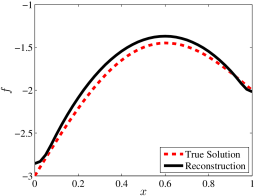
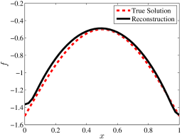
Figure 1: True solutions $f_{\mathrm{true}}$ and their reconstructions $f_{K}$ obtained in Example 5.1. Left: Case (a), $K=16$, $\mathrm{err}=4.56\%$; Right: Case (b), $K=49$, $\mathrm{err}=4.92\%$.

Example 5.2

In this example, we fix $\alpha=0.8$, $M=1$ and the true solution $f_{\mathrm{true}}(x)=-\sin(\pi x/2)-x^{2}+3$. Our aim is to test the numerical performance of Algorithm 4.5 with various choices of the noise level $\delta$ and the observation subdomain $\omega$ to see their influences on the reconstructions. First we fix $\omega=(0,0.05)\cup(0.95,1)$ and enlarge $\delta$ from $0.5\%$, $1\%$, $2\%$ to $4\%$. Next, we fix the noise level as $\delta=2\%$ and shrink $\omega$ from $(0,0.2)\cup(0.8,1)$, $(0,0.1)\cup(0.9,1)$ to $(0,0.025)\cup(0.975,1)$. The choices of $\delta$, $\omega$ in the tests and the corresponding numerical performances are listed in Table 1.

Table 1: Choices of noise levels $\delta$ and observation subdomains $\omega$ along with the corresponding iteration steps $K$ and the relative errors $\mathrm{err}$ in Example 5.2.

$\delta$	$\omega$	$\mathrm{err}$	$K$
$0.5\%$	$(0,0.05)\cup(0.95,1)$	$2.87\%$	$51$
$1\%$	$(0,0.05)\cup(0.95,1)$	$3.61\%$	$51$
$2\%$	$(0,0.05)\cup(0.95,1)$	$5.38\%$	$51$
$4\%$	$(0,0.05)\cup(0.95,1)$	$9.35\%$	$50$
$2\%$	$(0,0.2)\cup(0.8,1)$	$4.11\%$	$20$
$2\%$	$(0,0.1)\cup(0.9,1)$	$4.05\%$	$31$
$2\%$	$(0,0.025)\cup(0.975,1)$	$9.89\%$	$79$

We can see from Figures 1 that with different fractional orders $\alpha$ and a $2\%$ noise in the data, the numerical reconstruction $f_{K}$ appear to be quite satisfactory in view of the highly ill-posedness of the inverse source problem, even with very bad initial constant guesses and very small sizes of the observation subdomain $\omega$. What’s more, we can observe from Table 1 that Algorithm 4.5 have two important advantages, namely, it processes strong robustness against the oscillating measurement errors, and it is not sensitive to the smallness of the observation subdomain $\omega$.

Now we proceed to the more challenging two-dimensional case, where we divide the space-time region $\overline{\Omega}\times[0,T]=[0,1]^{2}\times[0,1]$ into a $40^{2}\times 40$ equidistant mesh. Similarly to the one-dimensional examples, we will test the numerical performance of Algorithm 4.5 from various aspects, including different choices of true solutions, noise levels and observation subdomains. For simplicity, we unify the tuning parameter in Algorithm 4.5 as $M=2$ in the following examples.

Example 5.3

Fix the noise level as $\delta=1\%$. We choose the observation subdomain and the tolerance parameter as $\omega=\Omega\setminus[0.1,0.9]^{2}$ and $\varepsilon=\delta/3$, respectively. We specify two pairs of fractional orders and true solutions as follows.

(a) $\alpha=0.3$, $f_{\mathrm{true}}(x)=f_{\mathrm{true}}(x_{1},x_{2})=x_{1}+x_{2}+1$.

(b) $\alpha=0.5$, $f_{\mathrm{true}}(x)=\cos(\pi x_{1})\cos(\pi x_{2})+2$.

Parallelly to Example 5.1, we compare the recovered solutions with the true ones, and show the iteration steps $K$ and the relative error $\mathrm{err}$ in Figure 2.

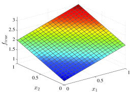
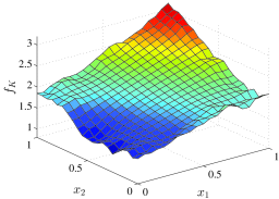
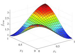
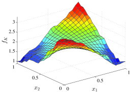
Figure 2: True solutions $f_{\mathrm{true}}$ (left) and their reconstructions $f_{K}$ (right) obtained in Example 5.3. Top: Case (a), $K=21$, $\mathrm{err}=6.21\%$; Bottom: Case (b), $K=36$, $\mathrm{err}=7.17\%$.

Example 5.4

The aim of this example is the same as that of Example 5.2, that is, to see the behavior of the reconstructions with respect to various choices of noise levels $\delta$ and observation subdomains $\omega$. To this end, we fix the fractional order $\alpha=0.8$ and the true solution $f_{\mathrm{true}}(x)=\exp((x_{1}+x_{2})/2)+1$, and choose the tolerance parameter as $\varepsilon=\delta/5$. First, we fix $\omega=\Omega\setminus[0.1,0.9]^{2}$ as that in the previous example, and change the noise levels as $\delta=0.5\%$, $1\%$, $2\%$ and $4\%$. Next, we fix $\delta=1\%$ and take $\omega$ as $\Omega\setminus[0.1,0.8]^{2}$, $\Omega\setminus[0.05,0.95]^{2}$ and $\Omega\setminus[0,0.9]\times[0.1,0.9]$. Especially, we see that in the last choice, $\omega$ only covers three edges of $\partial\Omega$. We list the choices of $\delta$, $\omega$ in the tests and the corresponding numerical performances in Table 2.

Table 2: Choices of noise levels $\delta$ and observation subdomains $\omega$ along with the corresponding iteration steps $K$ and the relative errors $\mathrm{err}$ in Example 5.4.

$\delta$	$\omega$	$\mathrm{err}$	$K$
$0.5\%$	$\Omega\setminus[0.1,0.9]^{2}$	$3.25\%$	$35$
$1\%$	$\Omega\setminus[0.1,0.9]^{2}$	$4.69\%$	$26$
$2\%$	$\Omega\setminus[0.1,0.9]^{2}$	$7.11\%$	$17$
$4\%$	$\Omega\setminus[0.1,0.9]^{2}$	$10.31\%$	$8$
$1\%$	$\Omega\setminus[0.1,0.8]^{2}$	$3.63\%$	$21$
$1\%$	$\Omega\setminus[0.05,0.95]^{2}$	$6.70\%$	$42$
$1\%$	$\Omega\setminus[0,0.9]\times[0.1,0.9]$	$5.46\%$	$22$

It can be readily seen from the above two-dimensional examples that the iterative thresholding algorithm shows almost the same numerical performances as that in the one-dimensional case. As expected, the proposed algorithm demonstrates a strong robustness against oscillating noises in the observation data and a certain insensitivity to the smallness of the observation subdomain. Nevertheless, we point out that the reconstructions here are not as accurate as that in [20], where a similar iterative method was applied to an inverse source problem for hyperbolic-type equations. The reason most probably roots in the underlying ill-posedness of Problem 1.2 for fractional parabolic equations, which is severer than that for hyperbolic ones.

sectionConcluding Remarks

2.3ex plus.2ex

In Theorem 2.6, we only proved the uniqueness result for the inverse source problem. In comparison, it is known that conditional stability results hold for the same inverse problems for parabolic or hyperbolic equations based on Carleman estimates or the multiplier method. Unfortunately, such techniques do not work in the case of fractional diffusion equations due to the absence of the fundamental integration by parts for the fractional derivatives. This is also a direct reason why the unique continuation was only established in the weak sense (see Theorem 2.5, Cheng et al. [4], Lin and Nakamura [17]) and Xu et al. [31]).

In the numerical aspect, we reformulate Problem 1.2 as a minimization problem in the typical situation in the case of $B\equiv 0$ and $m=1$. Then we characterize the minimizer by a variational with the help of the corresponding adjoint problem of (1.2), which results in the desired iterative thresholding algorithm. Then several numerical experiments for the reconstructions are implemented to show the efficiency and accuracy of the proposed Algorithm 4.5. Here we point out that in case of the homogeneous Neumann boundary condition, it is necessary to assume $B=0$ in Algorithm 4.5, since the adjoint system used to derive our algorithm heavily relies on the symmetry of problem (4.1). The algorithm for the non-symmetric case remains open.

sectionProof of Lemma 2.4

2.3ex plus.2ex

In this appendix, we provide the proof of Lemma 2.4, namely, the well-posedness of the weak solution to the inhomogeneous problem (1.2) in the sense of fractional Sobolev spaces in time. To this end, we introduce the usual Mittag-Leffler function (see, e.g., [26, §1.2.1])

$$E_{\alpha,\beta}(\zeta):=\sum_{k=1}^{\infty}\frac{\zeta^{k}}{\Gamma(\alpha k+\beta)},\quad\zeta\in\mathbb{C},\ \alpha>0,\ \beta\in\mathbb{R},$$

by which we define a collection of solution operators $\{S_{\alpha}(t)\}_{t>0}$ as

$$S_{\alpha}(t):L^{2}(\Omega) \to L^{2}(\Omega),$$ (A.1)

$$\psi \mapsto-t^{\alpha-1}\sum_{n=1}^{\infty}E_{\alpha,\alpha}(-\lambda_{n}t^{\alpha})(\psi,\varphi_{n})\varphi_{n}.$$

Moreover, it follows from [26, Theorem 1.6] that there exists a constant $C>0$ such that

$$\|S_{\alpha}(t)\|_{\mathrm{op}}\leq C\,t^{\alpha-1},\quad t>0.$$ (A.2)

We are in a position to give the proof of Lemma 2.4.

Proof of Lemma 2.4.

Let $a=0$ and $F\in L^{2}(Q)$. Without loss of generality, we only treat the multi-term case, i.e., $m\geq 2$. Henceforth, $C>0$ denotes generic constants which may change from line to line.

Regarding the terms of lower fractional orders and advection as the new source terms, we can argue similarly as that in the proof in [13] to see that the solution formally satisfies the integral equation

$$u(\,\cdot\,,t)=(\mathcal{K}-\mathcal{L})u(\,\cdot\,,t)-\Psi(\,\cdot\,,t),$$

where

$$\mathcal{K}:=\sum_{j=2}^{m}q_{j}\mathcal{K}_{j},\quad\mathcal{K}_{j}u(\,\cdot\,,t):=\int_{0}^{t}S_{\alpha_{1}}(t-\tau)\partial_{\tau}^{\alpha_{j}}u(\,\cdot\,,\tau)\,\mathrm{d}\tau\ (j=2,\ldots,m),$$

$$\mathcal{L}u(\,\cdot\,,t):=\int_{0}^{t}S_{\alpha_{1}}(t-\tau)B\cdot\nabla u(\,\cdot\,,\tau)\,\mathrm{d}\tau,\quad\Psi(\,\cdot\,,t):=\int_{0}^{t}S_{\alpha_{1}}(t-\tau)F(\,\cdot\,,\tau)\,\mathrm{d}\tau.$$

In the sequel, for $\eta\in(0,T]$ we define the space $X_{\eta}$ and its norm $\|\cdot\|_{X_{\eta}}$ as

$$X_{\eta}:=H^{\alpha_{1}}(0,\eta;L^{2}(\Omega))\cap L^{2}(0,\eta;H^{2}(\Omega)),\quad\|\cdot\|_{X_{\eta}}:=\|\cdot\|_{H^{\alpha_{1}}(0,\eta;L^{2}(\Omega))}+\|\cdot\|_{L^{2}(0,\eta;H^{2}(\Omega))},$$

respectively. Recalling the operator $\widetilde{\mathcal{A}}$ introduced in Section Weak Unique Continuation Property and a Related Inverse Source Problem for Time-Fractional Diffusion-Advection Equations, we have $\widetilde{\mathcal{A}}\Psi=\mathcal{A}\Psi+\Psi$, where

$$\mathcal{A}\Psi(\,\cdot\,,t)=\int_{0}^{t}(t-\tau)^{\alpha_{1}-1}\sum_{n=1}^{\infty}\lambda_{n}E_{\alpha_{1},\alpha_{1}}(-\lambda_{n}(t-\tau)^{\alpha_{1}})(F(\,\cdot\,,\tau),\varphi_{n})\varphi_{n}\,\mathrm{d}s$$

by definition (A.1). First it follows immediately from (A.2) and Young’s inequality that

$$\|\Psi\|_{L^{2}(\Omega\times(0,\eta))}\leq C\|F\|_{L^{2}(\Omega\times(0,\eta))}.$$

To estimate $\mathcal{A}\Psi$, we take advantage of the basic properties of Mittag-Leffler functions (see, e.g., [27, Lemma 3.3]) to deduce

$$\lambda_{n}\int_{0}^{\eta}t^{\alpha_{1}-1}|E_{\alpha_{1},\alpha_{1}}(-\lambda_{n}t^{\alpha_{1}})|\,\mathrm{d}t =\lambda_{n}\int_{0}^{\eta}t^{\alpha_{1}-1}E_{\alpha_{1},\alpha_{1}}(-\lambda_{n}t^{\alpha_{1}})\,\mathrm{d}t$$

$$=-\int_{0}^{\eta}\frac{\mathrm{d}}{\mathrm{d}t}E_{\alpha_{1},1}(-\lambda_{n}t^{\alpha_{1}})\,\mathrm{d}t=1-E_{\alpha_{1},1}(-\lambda_{n}\eta^{\alpha_{1}}).$$

From the boundedness of $E_{\alpha_{1},1}(-\lambda_{n}\eta^{\alpha_{1}})$ and Young’s inequality, we obtain

$$\|\mathcal{A}\Psi\|_{L^{2}(\Omega\times(0,\eta))}\leq\sum_{n=1}^{\infty}\left(\int_{0}^{\eta}|(F(\,\cdot\,,t),\varphi_{n})|^{2}\,\mathrm{d}t\right)^{1/2}(1-E_{\alpha_{1},1}(-\lambda_{n}\eta^{\alpha_{1}}))\leq C\|F\|_{L^{2}(\Omega\times(0,\eta))},$$

indicating

$$\|\Psi\|_{L^{2}(0,\eta;H^{2}(\Omega))}\leq C\|F\|_{L^{2}(\Omega\times(0,\eta))}.$$

Now by an argument similar to the proof of [7, Theorem 4.1], we obtain

$$\|\Psi\|_{H^{\alpha_{1}}(0,\eta;L^{2}(\Omega))}\leq C\|F\|_{L^{2}(\Omega\times(0,\eta))}.$$

Next we proceed to show that $\mathcal{K}-\mathcal{L}:X_{\eta}\to X_{\eta}$ is compact. In fact, according to [7, Theorem 4.2], we have

$$\|\mathcal{L}w\|_{X_{\eta}}\leq C\|B\cdot\nabla w\|_{L^{2}(\Omega\times(0,\eta))}\leq C\|w\|_{L^{2}(0,\eta;H^{1}(\Omega))},\quad\forall\,w\in X_{\eta},$$ (A.3)

that is, $\mathcal{L}:L^{2}(0,\eta;H^{1}(\Omega))\to X_{\eta}$ is bounded. Since the embedding $X_{\eta}\to L^{2}(0,\eta;H^{1}(\Omega))$ is compact, we immediately obtain the compactness of the operator $\mathcal{L}:X_{\eta}\to X_{\eta}$. On the other hand, by $1>\alpha_{1}>\alpha_{2}>\cdots>\alpha_{m}>0$, we see

$$\|\mathcal{K}_{j}w\|_{X_{\eta}}\leq C\|w\|_{H^{\alpha_{j}}(0,\eta;L^{2}(\Omega))}\leq C\|w\|_{H^{\alpha_{2}}(0,\eta;L^{2}(\Omega))},\quad\forall\,w\in X_{\eta},\ j=2,\ldots,m,$$ (A.4)

where the constant $C>0$ is independent of $\eta\in(0,T)$ (see [27, p.434]). Meanwhile, the embedding $X_{\eta}\to H^{\alpha_{2}}(0,\eta;L^{2}(\Omega))$ is compact (see Temam [30, Chapter III, §2], or one can prove directly similarly to Baumeister [3, Chapter 5]), which yields the compactness of $\mathcal{K}=\sum_{j=2}^{m}q_{j}\mathcal{K}_{j}:X_{\eta}\to X_{\eta}$ and thus the compactness of $\mathcal{K}-\mathcal{L}:X_{\eta}\to X_{\eta}$.

Now we attempt to verify that $1$ is not an eigenvalue of $\mathcal{K}-\mathcal{L}$, that is, $(\mathcal{K}-\mathcal{L})w=w$ in $X_{\eta}$ implies $w=0$. First we prove

$$\|\partial_{t}^{\beta}g\|_{L^{2}(0,\eta)}\leq C\,\eta^{\alpha_{1}-\beta}\|\partial_{t}^{\alpha_{1}}g\|_{L^{2}(0,\eta)},\quad\forall\,\beta\in[0,\alpha_{1}),\ \forall\,g\in\mathcal{R}(J_{0+}^{\alpha_{1}}).$$ (A.5)

Indeed, since $J_{0+}^{\gamma}$ is defined by the fractional power for $\gamma\in\mathbb{R}$, if follows that (see Pazy [25, Theorem 6.8])

$$J_{0+}^{-\beta}g=J_{0+}^{\alpha_{1}-\beta}(J_{0+}^{-\alpha_{1}}g),\quad g\in\mathcal{R}(J_{0+}^{\alpha_{1}})$$

and thus

$$\|\partial_{t}^{\beta}g\|_{L^{2}(0,\eta)}=\|J_{0+}^{-\beta}g\|_{L^{2}(0,\eta)}=\|J_{0+}^{\alpha_{1}-\beta}(J_{0+}^{-\alpha_{1}}g)\|_{L^{2}(0,\eta)},\quad g\in\mathcal{R}(J_{0+}^{\alpha_{1}}).$$

On the other hand, by Young’s inequality, there holds for $g\in\mathcal{R}(J_{0+}^{\alpha_{1}})\subset H^{\alpha_{1}}(0,\eta)$ that

$$\|J_{0+}^{\alpha_{1}-\beta}g\|_{L^{2}(0,\eta)} =\frac{1}{\Gamma(\alpha_{1}-\beta)}\left\|\int^{t}_{0}(t-\tau)^{(\alpha_{1}-\beta)-1}g(\tau)\,\mathrm{d}\tau\right\|_{L^{2}(0,\eta)}$$

$$\leq\frac{1}{\Gamma(\alpha_{1}-\beta)}\int_{0}^{\eta}t^{(\alpha_{1}-\beta)-1}\,\mathrm{d}t\left(\int_{0}^{\eta}|g(t)|^{2}\,\mathrm{d}t\right)^{1/2}=\frac{\eta^{\alpha_{1}-\beta}}{\Gamma(\alpha_{1}-\beta+1)}\|g\|_{L^{2}(0,\eta)},$$

implying

$$\|\partial_{t}^{\beta}g\|_{L^{2}(0,\eta)}\leq C\,\eta^{\alpha_{1}-\beta}\|J_{0+}^{-\alpha_{1}}g\|_{L^{2}(0,\eta)}=C\,\eta^{\alpha_{1}-\beta}\|\partial_{t}^{\alpha_{1}}g\|_{L^{2}(0,\eta)}$$

or equivalently (A.5). Using (A.4) and (A.5), we estimate

$$\|\mathcal{K}_{j}w\|_{X_{\eta}} \leq C\|\partial_{t}^{\alpha_{j}}w\|_{L^{2}(\Omega\times(0,\eta))}\leq C\,\eta^{\alpha_{1}-\alpha_{j}}\|\partial_{t}^{\alpha_{1}}w\|_{L^{2}(\Omega\times(0,\eta))}$$

$$\leq C\,\eta^{\alpha_{1}-\alpha_{2}}\|w\|_{H^{\alpha_{1}}(0,\eta;L^{2}(\Omega))}\leq C\,\eta^{\alpha_{1}-\alpha_{2}}\|w\|_{X_{\eta}},\quad\forall\,w\in X_{\eta},\ j=2,\ldots,m.$$ (A.6)

Especially, taking $\beta=0$ in (A.5), we obtain

$$\|w\|_{L^{2}(\Omega\times(0,\eta))}\leq C\,\eta^{\alpha_{1}}\|\partial_{t}^{\alpha_{1}}w\|_{L^{2}(\Omega\times(0,\eta))}\leq C\,\eta^{\alpha_{1}}\|w\|_{X_{\eta}},\quad\forall\,w\in X_{\eta}.$$

Applying the above estimate and the interpolation inequality to (A.3), we see that for any $\epsilon>0$, there exists a constant $C_{\epsilon}>0$ such that

$$\|\mathcal{L}w\|_{X_{\eta}} \leq C\|w\|_{L^{2}(0,\eta;H^{1}(\Omega))}\leq\epsilon\|w\|_{L^{2}(0,\eta;H^{2}(\Omega))}+C_{\epsilon}\|w\|_{L^{2}(\Omega\times(0,\eta))}$$

$$\leq(\epsilon+CC_{\epsilon}\,\eta^{\alpha_{1}})\|w\|_{X_{\eta}},\quad\forall\,w\in X_{\eta}.$$

This, together with the estimate (A.6), implies

$$\|(\mathcal{K}-\mathcal{L})w\|_{X_{\eta}} \leq\sum_{j=2}^{m}q_{j}\|\mathcal{K}_{j}w\|_{X_{\eta}}+\|\mathcal{L}w\|_{X_{\eta}}\leq\left(C\,\eta^{\alpha_{1}-\alpha_{2}}+\epsilon+CC_{\epsilon}\,\eta^{\alpha_{1}}\right)\|w\|_{X_{\eta}},\quad\forall\,w\in X_{\eta}.$$

Fixing $0<\epsilon<1$ arbitrarily, we can choose a sufficiently small $\eta_{\epsilon}>0$ so that

$$C\,\eta_{\epsilon}^{\alpha_{1}-\alpha_{2}}+\epsilon+CC_{\epsilon}\,\eta_{\epsilon}^{\alpha_{1}}<1.$$

Consequently, if $w=(\mathcal{K}-\mathcal{L})w$ in $X_{\eta_{\epsilon}}$, then the only possibility is $w=0$ in $\Omega\times(0,\eta_{\epsilon})$, indicating that $1$ is not an eigenvalue of $\mathcal{K}-\mathcal{L}$ on $X_{\eta_{\epsilon}}$.

In the final step, we continue this argument over $\eta_{\epsilon}$ to show that $w=(\mathcal{K}-\mathcal{L})w$ in $X_{2\eta_{\epsilon}}=H^{\alpha_{1}}(0,2\eta_{\epsilon};L^{2}(\Omega))\cap L^{2}(0,2\eta_{\epsilon};H^{2}(\Omega))$ implies $w=0$ in $\Omega\times(0,2\eta_{\epsilon})$. To this end, we investigate $\widetilde{w}(\,\cdot\,,t):=w(\,\cdot\,,t+\eta_{\epsilon})$. Now that $w=0$ in $\Omega\times(0,\eta_{\epsilon})$, formally we calculate

$$\partial_{t}^{\alpha_{j}}w(\,\cdot\,,t+\eta_{\epsilon}) =\frac{1}{\Gamma(1-\alpha_{j})}\int_{\eta_{\epsilon}}^{t+\eta_{\epsilon}}\frac{\partial_{\tau}w(\,\cdot\,,\tau)}{(t+\eta_{\epsilon}-\tau)^{\alpha_{j}}}\,\mathrm{d}\tau=\frac{1}{\Gamma(1-\alpha_{j})}\int_{0}^{t}\frac{\partial_{\xi}w(\,\cdot\,,\xi+\eta_{\epsilon})}{(t-\xi)^{\alpha_{j}}}\,\mathrm{d}\xi$$

$$=\frac{1}{\Gamma(1-\alpha_{j})}\int_{0}^{t}\frac{\partial_{\xi}\widetilde{w}(\,\cdot\,,\xi)}{(t-\xi)^{\alpha_{j}}}\,\mathrm{d}\xi=\partial_{t}^{\alpha_{j}}\widetilde{w}(\,\cdot\,,t),\quad t>0.$$

By the definition of $\mathcal{K}_{j}$, we employ again the fact that $w=0$ in $\Omega\times(0,\eta_{\epsilon})$ to deduce

$$\mathcal{K}_{j}w(\,\cdot\,,t+\eta_{\epsilon}) =\int_{0}^{t+\eta_{\epsilon}}S_{\alpha_{1}}(t+\eta_{\epsilon}-\tau)\partial_{\tau}^{\alpha_{j}}w(\,\cdot\,,\tau)\,\mathrm{d}\tau=\int_{\eta_{\epsilon}}^{t+\eta_{\epsilon}}S_{\alpha_{1}}(t+\eta_{\epsilon}-\tau)\partial_{\tau}^{\alpha_{j}}w(\,\cdot\,,\tau)\,\mathrm{d}\tau$$

$$=\int_{0}^{t}S_{\alpha_{1}}(t-\xi)\partial_{\xi}^{\alpha_{j}}w(\,\cdot\,,\xi+\eta_{\epsilon})\,\mathrm{d}\xi=\int_{0}^{t}S_{\alpha_{1}}(t-\xi)\partial_{\xi}^{\alpha_{j}}\widetilde{w}(\,\cdot\,,\xi)\,\mathrm{d}\xi$$

$$=\mathcal{K}_{j}\widetilde{w}(\,\cdot\,,t),\quad t>0,\ j=2,\ldots,m.$$

Similarly, we obtain

$$\mathcal{L}w(\,\cdot\,,t+\eta_{\epsilon})=\mathcal{L}\widetilde{w}(\,\cdot\,,t),\quad t>0.$$

Eventually, we collect the above equalities to conclude

$$\widetilde{w}(\,\cdot\,,t) =w(\,\cdot\,,t+\eta_{\epsilon})=\sum_{j=2}^{m}q_{j}\mathcal{K}_{j}w(\,\cdot\,,t+\eta_{\epsilon})-\mathcal{L}w(\,\cdot\,,t+\eta_{\epsilon})$$

$$=\sum_{j=2}^{m}q_{j}\mathcal{K}_{j}\widetilde{w}(\,\cdot\,,t)-\mathcal{L}\widetilde{w}(\,\cdot\,,t)=(\mathcal{K}-\mathcal{L})\widetilde{w}(\,\cdot\,,t),\quad t>0.$$

Therefore, the same argument for $w\in X_{\eta}$ immediately yields $\widetilde{w}=0$ in $\Omega\times(0,\eta_{\epsilon})$ and thus $w=0$ in $\Omega\times(0,2\eta_{\epsilon})$. Since the step size $\eta_{\epsilon}$ is a positive constant, we can repeat the same argument finite times to reach the conclusion that $w=(\mathcal{K}-\mathcal{L})w$ in $X_{T}=H^{\alpha_{1}}(0,T;L^{2}(\Omega))\cap L^{2}(0,T;H^{2}(\Omega))$ implies $w=0$ in $Q=\Omega\times(0,T)$.

Consequently, by the Fredholm alternative, we complete the proof of Lemma 2.4. ∎

Acknowledgement  The work was supported by A3 Foresight Program “Modeling and Computation of Applied Inverse Problems”, Japan Society of the Promotion of Science (JSPS). The first author is supported by self-determined research funds of CCNU from the colleges’ basic research and operation of MOE (No.​ CCNU14A05039), National Natural Science Foundation of China (Nos.​ 11326233, 11401241 and 11571265). The second author is partially supported by the Program for Leading Graduate Schools, MEXT, Japan. The other authors are partially supported by Grant-in-Aid for Scientific Research (S) 15H05740, JSPS.

References

[1]
Adams E E and Gelhar L W 1992 Field study of dispersion in a heterogeneous
aquifer: 2. Spatial moments analysis Water Resour. Res.28 3293–307
[2]
Adams R A 1975 Sobolev Spaces (New York: Academic Press)
[4]
Cheng J, Lin C-L and Nakamura G 2013 Unique continuation property for the
anomalous diffusion and its application J. Differential Equations254 3715–28
[5]
Cheng J, Nakagawa J, Yamamoto M and Yamazaki T 2009 Uniqueness in an inverse
problem for a one-dimensional fractional diffusion equation Inverse
Problems25 115002
[6]
Daubechies I, Defrise M and De Mol C 2004 An iterative thresholding algorithm
for linear inverse problems Comm. Pure Appl. Math.57 1413–57
[7]
Gorenflo R, Luchko Y and Yamamoto M 2015 Time-fractional diffusion equation in
the fractional Sobolev spaces Frac. Calc. Appl. Anal.18 799–820
[8]
Fujishiro K 2014 Approximate controllability for fractional diffusion equations
by Dirichlet boundary control arXiv:1404.0207v3
[9]
Hatano Y and Hatano N 1998 Dispersive transport of ions in column experiments:
an explanation of long-tailed profiles Water Resour. Res.34
1027–33
[10]
Jin B, Lazarov R, Liu Y and Zhou Z 2015 The Galerkin finite element method for
a multi-term time-fractional diffusion equation J. Comput. Phys.281
825–43
[11]
Jin B, Lazarov R and Zhou Z 2013 Error estimates for a semidiscrete finite
element method for fractional order parabolic equations SIAM J. Numer.
Anal.51 445–66
[12]
Li Z, Liu Y and Yamamoto M 2015 Initial-boundary value problems for multi-term
time-fractional diffusion equations with positive constant coefficients Appl. Math. Comput.257 381–97
[13]
Li Z and Yamamoto M 2013 Initial-boundary value problems for linear diffusion
equation with multiple time-fractional derivatives arXiv:1306.2778v2
[14]
Li Z, Imanuvilov O and Yamamoto 2016 Uniqueness in inverse boundary value
problems for fractional diffusion equations Inverse Problems32
015004
[15]
Li Z and Yamamoto M 2015 Uniqueness for inverse problems of determining orders
of multi-term time-fractional derivatives of diffusion equation Appl.
Anal.94 570–9
[16]
Li G, Zhang D, Jia X and Yamamoto M 2013 Simultaneous inversion for the
space-dependent diffusion coefficient and the fractional order in the
time-fractional diffusion equation Inverse Problems29 065014
[17]
Lin C-L and Nakamura G 2016 Unique continuation property for anomalous slow
diffusion equation Commun. Partial Diff. Eqns at press
[18]
Lin Y and Xu C 2007 Finite difference/spectral approximations for the
time-fractional diffusion equation Appl. Math. Comput.225 1533–52
[19]
Liu Y 2015 Strong maximum principle for multi-term time-fractional diffusion
equations and its application to an inverse source problem arXiv:1510.06878
[20]
Liu Y, Jiang D and Yamamoto M 2015 Inverse source problem for a double
hyperbolic equation describing the three-dimensional time cone model SIAM
J. Appl. Math.75 2610–35
[21]
Liu Y, Rundell W and Yamamoto M 2016 Strong maximum principle for fractional
diffusion equations and an application to an inverse source problem, Frac.
Calc. Appl. Anal. (accepted)
[22]
Luchko Y 2010 Some uniqueness and existence results for the
initial-boundary-value problems for the generalized time-fractional diffusion
equation Comput. Math. Appl.59 1766–72
[23]
Luchko Y 2011 Initial-boundary-value problems for the generalized multi-term
time-fractional diffusion equation J. Math. Anal. Appl.374 538–48
[24]
Miller L and Yamamoto M 2013 Coefficient inverse problem for a fractional
diffusion equation Inverse Problems29 075013
[25]
Pazy A 1983 Semigroups of Linear Operators and Applications to Partial
Differential Equations (Berlin: Springer)
[26]
Podlubny I 1999 Fractional Differential Equations (San Diego: Academic)
[27]
Sakamoto K and Yamamoto M 2011 Initial value/boundary value problems for
fractional diffusion-wave equations and applications to some inverse problems
J. Math. Anal. Appl.382 426–47
[28]
Sakamoto K and Yamamoto M 2011 Inverse source problem with a final
overdetermination for a fractional diffusion equation Math. Control Relat.
Fields1 509–18
[29]
Saut J C and Scheurer B 1987 Unique continuation for some evolution equations
J. Differential Equations66 118–39
[30]
Temam R 1977 Navier-Stokes Equations: Theory and Numerical Analysis
(Amsterdam: North-Holland)
[31]
Xu X, Cheng J and Yamamoto M 2011 Carleman estimate for a fractional diffusion
equation with half order and application Appl. Anal.90 1355–71
[32]
Yamamoto M and Zhang Y 2012 Conditional stability in determining a zeroth-order
coefficient in a half-order fractional diffusion equation by a Carleman
estimate Inverse Problems28 105010
[33]
Zhang Z 2016 An undetermined coefficient problem for a fractional diffusion
equation Inverse Problems32 015011
[34]
Zhang Y and Xu X 2011 Inverse source problem for a fractional diffusion
equation Inverse Problems27 035010