Jastrow correlation factor for periodic systems

Abstract

We propose a Jastrow factor for electron-electron correlations that interpolates between the radial symmetry of the Coulomb interaction at short inter-particle distance and the space-group symmetry of the simulation cell at large separation. The proposed Jastrow factor captures comparable levels of the correlation energy to current formalisms, is 40% quicker to evaluate, and offers benefits in ease of use, as we demonstrate in quantum Monte Carlo simulations.

I Introduction

Quantum Monte Carlo (QMC) is a prominent family of techniques for studying strong correlations in quantum many-body systems Foulkes01 . In particular, the variational and diffusion Monte Carlo methods (VMC and DMC) are accurate tools for studying ground-state energies and expectation values. Both methods are predicated on the use of a trial wavefunction, whose similarity to the true ground state determines the accuracy and efficiency of the calculations Reynolds82 . It is therefore important to have access to a high fidelity trial wavefunction.

A common foundation for constructing a fermionic trial wavefunction is to begin with the Hartree–Fock wavefunction $\Psi_{\mathrm{HF}}=D_{\uparrow}D_{\downarrow}$, where $D_{\uparrow}$ ($D_{\downarrow}$) is a Slater determinant of single-electron states for the up (down) spin species. The Slater determinants encode the fermionic antisymmetry of the trial wavefunction, ensuring Pauli exchange is satisfied, but do not include any effects of electron correlation. To describe such correlations, we modify the trial wavefunction to be of the Slater–Jastrow Jastrow55 form $\Psi=\mathrm{e}^{J(\mathbf{R})}D_{\uparrow}D_{\downarrow}$, where $\mathrm{e}^{J(\mathbf{R})}$ is a Jastrow factor that is a function of all the electron positions, $\mathbf{R}$. For real $J(\mathbf{R})$ the Jastrow factor is positive definite, and hence does not modify the nodal structure of the Hartree–Fock wavefunction.

In order to allow the Jastrow factor to accurately describe the correlations in a particular system of interest, $J(\mathbf{R})$ depends on a number of variational parameters McMillan65 ; Williamson96 ; Drummond04 ; Rios12 ; Ortiz94 ; Ceperley78 ; Guclu05 ; Astrakharchik07 . These parameters can be optimized using the relatively inexpensive VMC method, and then the optimal trial wavefunction used as the starting point for a more accurate but more expensive DMC calculation. In principle the DMC estimate of the energy depends only on the nodal surface of the trial wavefunction Anderson76 , but in practice a more accurate trial wavefunction with an optimized Jastrow factor allows the method to proceed more efficiently.

In this paper we consider Jastrow factors for infinite, periodic systems. These systems are amenable to numerical simulation through the use of finite simulation cells which are tessellated, with periodic boundary conditions, to fill all of space. Jastrow factors in the literature tend to either respect the short range radial symmetry of the Coulomb interaction, or abide by the symmetry of the simulation cells, but not both Williamson96 ; Drummond04 ; Rios12 ; Ortiz94 . Here we propose a Jastrow factor that interpolates between these symmetries; is easier to use than current Jastrow factors by virtue of having a single parameter that tunes its accuracy, as opposed to two such parameters for other Jastrow factors of similar accuracy; requires fewer variational parameters to reach comparable accuracy; and is 40% quicker to evaluate than these current Jastrow factors.

All of our QMC simulations were performed using the casino package Needs10 , and we use Hartree atomic units throughout this paper. In Section II we review common Jastrow factors from the literature, and then show how our proposed Jastrow factor fits into this hierarchy. In Section III and Section IV we examine the accuracy and efficiency of the Jastrow factors in the homogeneous electron gas and crystalline beryllium, respectively, before drawing our conclusions in Section V.

II Jastrow factor

We are concerned with Jastrow factors that capture correlation between electrons, and hence include functions of electron-electron separation,

$$J(\mathbf{R})=\sum_{\begin{subarray}{c}j>i\\ \sigma,\tau\in\{\uparrow,\downarrow\}\end{subarray}}J_{\sigma\tau}(\mathbf{r}_{ij}),$$

where $\mathbf{r}_{ij}=\mathbf{r}_{i}-\mathbf{r}_{j}$, the sum runs over all electrons labeled $i$, $j$, and we refer to $J_{\sigma\tau}(\mathbf{r}_{ij})$ as a Jastrow function. The Jastrow function contains variational parameters that we optimize within a VMC calculation to minimize the variance in the local energy Umrigar88 .

There are some fundamental constraints on the form of the Jastrow function. Firstly, in order to retain the spin expectation value of the Hartree–Fock wavefunction $J_{\sigma\tau}(\mathbf{r}_{ij})$ must be even under exchange of particles. Secondly, in order to avoid non-physical divergences in the local energy, $J_{\sigma\tau}(\mathbf{r}_{ij})$ must be at least twice-differentiable everywhere except at particle coalescence ($\mathbf{r}_{ij}=\boldsymbol{0}$).

However, at particle coalescence the Coulombic potential energy of two electrons diverges. In order to retain a non-divergent local energy the kinetic energy therefore has to diverge in the opposite direction at particle coalescence. This may be achieved by imposing the Kato cusp conditions Kato57 on the wavefunction, which may be expressed as

$$\left.\frac{\partial J_{\sigma\tau}}{\partial r_{ij}}\right|_{r_{ij}=0}=\Gamma_{\sigma\tau},$$

giving spherically-symmetric behavior at short radius $J_{\sigma\tau}(\mathbf{r}_{ij})=\Gamma_{\sigma\tau}r_{ij}+\ldots$, where, for 3D systems, $\Gamma_{\uparrow\uparrow}=\Gamma_{\downarrow\downarrow}=\frac{1}{4}$ and $\Gamma_{\uparrow\downarrow}=\Gamma_{\downarrow\uparrow}=\frac{1}{2}$. The final constraint on the Jastrow factor is that, in periodic systems like those we consider here, $J_{\sigma\tau}(\mathbf{r}_{ij})$ must satisfy periodic boundary conditions at the edge of the simulation cell in order to tessellate space.

Before presenting and testing our proposal for a Jastrow factor, we first review other Jastrow factors that are commonly used in the literature. We organize the Jastrow factors by their symmetry, starting with a spherically symmetric function and then examining a Jastrow factor with the symmetry of the simulation cell before proposing our Jastrow factor that interpolates between these symmetries.

II.1 Term with spherical symmetry

The interaction between two isolated electrons is isotropic, and so it is reasonable to take the Jastrow factor as being spherically symmetric and purely a function of particle separation where two-body effects dominate, and especially at inter-particle separations shorter than the average nearest-neighbor separation in many-body systems. However, the simulation cells used in numerical calculations are not spherically symmetric as they have to tessellate to fill 3D space. Because of this requirement, and in order to limit the effect of otherwise infinite-ranged terms to within the simulation cell, radial terms in the Jastrow factor are cut off at a finite radius that is less than or equal to the Wigner–Seitz radius corresponding to the simulation cell. This is implemented by including a term $(1-r_{ij}/L_{\sigma\tau})^{C}\Theta(L_{\sigma\tau}-r_{ij})$ in the Jastrow function, which goes to zero at a radius $L_{\sigma\tau}$, with $C-1$ continuous derivatives. We take $C=3$ in order to keep the local energy continuous at the cutoff radius Drummond04 . $\Theta(L_{\sigma\tau}-r_{ij})$ is a Heaviside step function, which forces the Jastrow function to be zero everywhere beyond the radius $L_{\sigma\tau}$.

It has been found in the literature Drummond04 ; Rios12 ; AlHamdani14 ; Chen14 ; Gillan15 that a Taylor expansion in electron-electron separation captures the most important short-ranged isotropic inter-particle correlations, and so here we review that expansion. Writing the Jastrow correlation function as a Taylor series around particle coalescence results in an expression

$$u_{\sigma\tau}(r_{ij})= \left(\frac{L_{\sigma\tau}}{3}\left[\alpha_{1,\sigma\tau}-\Gamma_{\sigma\tau}\right]+\sum_{m=1}^{N_{\mathrm{u}}}\alpha_{m,\sigma\tau}r_{ij}^{m}\right)\times$$

$$\times\left(1-r_{ij}/L_{\sigma\tau}\right)^{3}\Theta\left(L_{\sigma\tau}-r_{ij}\right),$$ (1)

which is referred to as a $u$ term Drummond04 ; Rios12 . Here the $N_{\mathrm{u}}$ coefficients $\alpha_{m,\sigma\tau}$ are parameters that are optimized using VMC, and the cutoff length $L_{\sigma\tau}$ is also optimized variationally. The term $L_{\sigma\tau}[\alpha_{1,\sigma\tau}-\Gamma_{\sigma\tau}]/3$ ensures that the Kato cusp conditions are satisfied. Using a pseudopotential for the electron-electron interaction LloydWilliams15 would set $\Gamma_{\sigma\tau}=0$.

The $u$ term Jastrow function with parameters optimized for an homogeneous electron gas with $r_{\mathrm{s}}=4$ is shown in Fig. 1a. The short-range behavior of the $u$ term is linear to satisfy the Kato cusp condition, and then at large separation the cutoff function limits the range of the $u$ term to within the Wigner-Seitz radius of the simulation cell, shown as a gray arc in Fig. 1a. This not only limits the maximum range of the correlations that can be captured by the $u$ term, but also prevents it from capturing correlations in the corners of the simulation cell.

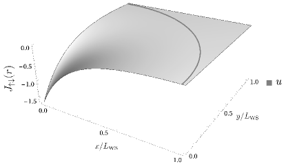
(a) $u$ term

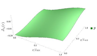
(b) $p$ term

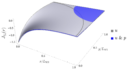
(c) $u$ and $u$ & $p$ terms

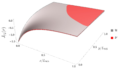
(d) $u$ and $\nu$ terms

Figure 1: (Color online) The Jastrow functions discussed in the main text, showing the (a) $u$, (b) $p$, (c) $u$ (gray) and $u$ & $p$ (blue), and (d) $u$ (gray) and $\nu$ (red) functions. The $u$, $u$ & $p$, and $\nu$ terms each have a total of five variational parameters, optimized using VMC in the homogeneous electron gas system. The data are taken for an opposite-spin electron pair in the $z=0$ plane, with one particle at the origin, showing one quadrant of the simulation cell. A gray arc indicates the $u$ term’s cutoff radius, which is comparable to the Wigner–Seitz radius $L_{\mathrm{WS}}$ of the simulation cell. We have subtracted a physically-irrelevant constant from the $\nu$ Jastrow function for clarity.

II.2 Term with simulation cell symmetry

One method to extend the ability of the Jastrow factor to capture correlations over the whole simulation cell is to use a form of Jastrow factor that innately has the space-group symmetry of the simulation cell. A simple but effective example of a Jastrow function that has such symmetry is a plane-wave basis, which also explicitly ensures periodicity of the Jastrow function. The so-called $p$ term takes the form Drummond04 ; Rios12

$$p_{\sigma\tau}(\mathbf{r}_{ij})=\sum_{\ell=1}^{N_{\mathrm{p}}}a_{\ell,\sigma\tau}\sum_{\mathbf{G}_{\ell}^{+}}\cos(\mathbf{G}_{\ell}\cdot\mathbf{r}_{ij}).$$ (2)

Here the $\{\mathbf{G}_{\ell}\}$ are the reciprocal lattice vectors of the simulation cell that belong to the $\ell^{\mathrm{th}}$ star of vectors equivalent under the full symmetry group of the simulation cell, sorted by increasing size of $|\mathbf{G}_{\ell}|$ (and in periodic systems not including the trivial vector $\boldsymbol{0}$); “$+$” means that if $\mathbf{G}_{\ell}$ is included in the sum, $-\mathbf{G}_{\ell}$ is excluded; and the $a_{\ell,\sigma\tau}$ are variational parameters, of which there are $N_{\mathrm{p}}$.

A $p$ term with $N_{\mathrm{p}}=1$ for the homogeneous electron gas is shown in Fig. 1b. The $p$ term exists over the whole simulation cell, including where the $u$ term is cut off to zero. This means the $p$ term can capture correlations in the cell corners that the $u$ term misses. However, the $p$ term does not tend to a radial form at short radius and so cannot satisfy the Kato cusp conditions at particle coalescence, meaning that on its own it does not make for an effective Jastrow factor. A common approach in the literature Conduit09 ; Drummond13 ; Whitehead16 ; Chiesa06 ; Spink13 ; Keyserlingk13 ; Maezono10 ; Mostaani15 is to combine both $u$ and $p$ terms to give a composite Jastrow function

$$J_{\sigma\tau}(\mathbf{r}_{ij})=u_{\sigma\tau}(r_{ij})+p_{\sigma\tau}(\mathbf{r}_{ij}),$$ (3)

which uses the $u$ term to capture short-range correlations and the Kato cusp conditions, and the $p$ term to capture long-range correlations in the corners of the simulation cell. We refer to such a combination as a $u$ & $p$ term.

An example of this composite Jastrow function, with $N_{\mathrm{u}}=3$ and $N_{\mathrm{p}}=1$ and parameters optimized in an homogeneous electron gas, is shown in Fig. 1c. As expected, the behavior at short range is dominated by the $u$ term. Yet at large radius this Jastrow function has structure due to the $p$ term, including in the corner of the simulation cell outside the cutoff radius of the $u$ term, shown by the gray arc, which allows the composite $u$ & $p$ term to capture longer-range correlations.

However, this construction has several undesirable features that limit its effectiveness at capturing inter-particle correlations. For a given amount of computing time to be spent optimizing the parameters in the Jastrow factor, a choice needs to be made of the relative number of $u$ and $p$ terms to be used. We do not know a priori the optimal ratio of $N_{\mathrm{u}}$ to $N_{\mathrm{p}}$, and so must explore a two-dimensional parameter space to determine it. A large proportion of the VMC calculation time is spent evaluating the Jastrow factor, and so it is important that the Jastrow factor is as simple as possible. But there is not equality of expense between the $u$ and $p$ terms, as sinusoidal $p$ terms are more expensive to calculate than polynomial $u$ terms, and the expense of a $p$ term also increases with the number of elements of the reciprocal lattice vector stars used to evaluate it. Higher-order stars generally contain more elements than lower-order ones, meaning high-order $p$ terms are even more expensive to calculate. To further complicate the optimization of the $u$ & $p$ term, although the $p$ term was intended to capture longer-range correlations, it does also exist at short radius; this means it interferes with the effect of higher-order contributions from the $u$ term.

One further problem with the form of Jastrow function given by Eq. (3) is that the cutoff length $L_{\sigma\tau}$ enters the expression non-linearly. To optimize the cutoff length and other parameters we need to solve a multi-dimensional non-linear set of equations, which is a significantly more difficult problem than solving a multi-dimensional linear set of equations, where the full force of linear algebra may be applied to increase the efficiency of the process Drummond05 .

We are interested in finding a form for the Jastrow factor that avoids these problems with the current method, by being a term with a single tuning parameter that determines the accuracy of the Jastrow factor, and which is also cheap to evaluate with linear coefficients. At the same time the proposed term should reproduce the advantageous properties of the $u$ term, accurately capturing short-range correlations, and also the $p$ term, exhibiting the symmetry of the simulation cell at large inter-particle separation.

II.3 $\nu$ term

We propose a Jastrow factor that combines the properties and symmetries of the $u$ term at small radius with the properties and symmetries of the $p$ term at large separation. The Jastrow function, referred to here as the $\nu$ term, is

$$\nu_{\sigma\tau}(\mathbf{r}_{ij}) =\sum_{n=1}^{N_{\nu}}c_{n,\sigma\tau}\left|f_{\mathrm{x}}^{2}(\mathbf{x}_{ij})+f_{\mathrm{y}}^{2}(\mathbf{y}_{ij})+f_{\mathrm{z}}^{2}(\mathbf{z}_{ij})\right|^{n/2},$$

$$f_{\mathrm{x}}(\mathbf{x}) =|\mathbf{x}|\left(1-\frac{|\mathbf{x}/L_{\mathrm{x}}|^{3}}{4}\right),$$ (4)

where the $N_{\nu}$ parameters $c_{n,\sigma\tau}$ are optimized using VMC, and the length $L_{\mathrm{x}}$ is the width of the simulation cell in the Cartesian $x$-direction. In Section IV.1 below we generalize the $\nu$ term to non-cuboidal geometries.

At small radius, the function $f_{\mathrm{x}}(\mathbf{x})=|\mathbf{x}|+O\left(|\mathbf{x}|^{4}\right)$, and so $|f_{\mathrm{x}}^{2}(\mathbf{x})+f_{\mathrm{y}}^{2}(\mathbf{y})+f_{\mathrm{z}}^{2}(\mathbf{z})|^{1/2}=r+O\left(r^{4}\right)$. This has the correct spherical symmetry to describe short-range electron-electron correlations, so at short radius the Jastrow function $\nu_{\sigma\tau}(\mathbf{r}_{ij})=\sum_{n=1}^{N_{\nu}}c_{n,\sigma\tau}r_{ij}^{n}+\ldots$ consists of an expansion in electron-electron separation, similarly to the $u$ term. This means the $\nu$ term will reproduce the ability of the $u$ term to capture short-ranged correlations and it is easy to satisfy the Kato cusp conditions by setting $c_{1,\sigma\tau}=\Gamma_{\sigma\tau}$.

The function $f(\mathbf{x})$ is symmetric under $\mathbf{x}\to-\mathbf{x}$, and automatically satisfies periodic boundary conditions at the edge of the simulation cell, with $f(L_{\mathrm{x}}\hat{\mathbf{x}})\neq 0$, $f^{\prime}(L_{\mathrm{x}}\hat{\mathbf{x}})=0$, and $f^{\prime\prime}(L_{\mathrm{x}}\hat{\mathbf{x}})\neq 0$: this is achieved through the use of the cubic power in the definition of $f$, chosen by analogy to the cutoff function in the $u$ term to distinguish long- and short-ranged components of the Jastrow function. Importantly, the $f$ functions satisfying periodic boundary conditions means any function constructed from them, such as the $\nu$ term, will also correctly satisfy periodic boundary conditions. The scaling of the $f$ functions in the different Cartesian directions lends the $\nu$ term the symmetry of the simulation cell at large inter-particle separation, and allows the $\nu$ term to capture long-range correlations, similarly to the $p$ term. Not requiring a cut-off function also means all the variational parameters enter the expression for $\nu_{\sigma\tau}(\mathbf{r}_{ij})$ linearly, and so are easier to optimize than the equivalent number of variational parameters in the $u$ term Drummond05 .

The $\nu$ Jastrow function optimized for a homogeneous electron gas is shown in Fig. 1d, demonstrating that it has the same small-radius behavior as the $u$ term. We can also see that the $\nu$ term still has structure in the corner of the simulation cell, similarly to the $u$ & $p$ term, which allows it to capture long-range inter-particle correlations. We will examine this similarity in more detail in a case study of the homogeneous electron gas in Section III.

Freedom to optimize the behavior of the Jastrow factor in the corners of the simulation cell also provides the freedom to change the kinetic energy of the wavefunction in the corners of the simulation cell, as $f_{\mathrm{x}}^{\prime\prime}(L_{\mathrm{x}}\hat{\mathbf{x}})\neq 0$. This allows the $\nu$ Jastrow factor to more accurately respond to a finite and/or varying potential energy in the corners of the simulation cell. From a Thomas–Fermi perspective this provides the $\nu$ term with the freedom to counteract changes in the potential energy from interactions with kinetic energy in order to keep the total energy constant.

The $\nu$ term may also be adapted to systems other than the 3D ones considered here. For 2D systems the $f_{\mathrm{z}}$ function may simply be omitted; or for slab geometries, with two directions periodic and one non-periodic, $f_{\mathrm{z}}$ should be replaced by a function that reduces to $|\mathbf{z}|$ at short radius, for example $|\mathbf{z}|\mathrm{e}^{-(|\mathbf{z}|/L_{\mathrm{z}})^{2}}$.

In order to demonstrate the advantages of the $\nu$ Jastrow factor, in the next two Sections we carry out simulations of the homogeneous electron gas and a crystalline solid. We examine the accuracy, efficiency, and ease of use of the $\nu$ Jastrow factor, and compare it with other forms of Jastrow factor used in the literature.

III Homogeneous electron gas

For the first test of our Jastrow factor we examine the homogeneous electron gas (HEG). This system has been widely studied using QMC Ceperley80 ; Zong02 ; Drummond04a ; Spink13 and serves as an analogue for electrons in a conductor. As it does not contain any atoms it allows us to focus on the electron-electron Jastrow factor. For simplicity we assume that the intra-species correlations for the up- and down-spin electrons are identical, and so fix $J_{\uparrow\uparrow}=J_{\downarrow\downarrow}$ and $J_{\uparrow\downarrow}=J_{\downarrow\uparrow}$.

We examine a HEG with density parameter $r_{\mathrm{s}}=4$ in a cubic simulation cell subject to periodic boundary conditions, and use Slater determinants of plane wave orbitals. We use a system of 57 up- and 57 down-spin electrons, and confirmed that the main results of this section were reproduced in systems of 33 and 81 electrons per spin species and so are independent of system size. We optimize all the Jastrow factors by minimizing the variance in the local energy Drummond05 ; Kent99 , and confirmed that minimizing the energy directly Umrigar07 gave similar results. All VMC simulations are run for $1\times 10^{6}$ steps. We then carry out DMC simulations to obtain a more accurate estimate for the energy within the fixed node approximation, $E_{\mathrm{DMC}}$, which corresponds to the use of a perfect Jastrow factor. DMC simulations starting with different trial wavefunctions agree to within $5\times 10^{-6}$ a.u. To measure the accuracy of the Jastrow factors, we evaluate the percentage of the DMC correlation energy missing from the VMC simulation,

$$\eta=\frac{E_{\mathrm{VMC}}-E_{\mathrm{DMC}}}{E_{\mathrm{HF}}-E_{\mathrm{DMC}}}\times 100\%$$

where the Hartree–Fock energy $E_{\mathrm{HF}}$ is that obtained by using just the Slater determinant part of the wavefunction.

In Fig. 2a we compare the percentages of the correlation energy missing when the various Jastrow factors under scrutiny are used. The horizontal axis is labeled by the number of optimizable parameters per spin channel, $N$, for each Jastrow function: so, for example, a $u$ term with a given number $N$ of optimizable parameters per spin channel has $N_{\mathrm{u}}=N-1$ optimizable parameters of terms in the inter-particle separation expansion, $\alpha_{m,\sigma\tau}$, as the cutoff length $L_{\sigma\tau}$ is also optimized. A $u$ & $p$ term with $N_{\mathrm{p}}$ optimizable parameters $a_{\ell,\sigma\tau}$ in the $p$ part leaves $N_{\mathrm{u}}=N-1-N_{\mathrm{p}}$ optimizable parameters for the $u$ term coefficients $\alpha_{m,\sigma\tau}$. For the $\nu$ term $N_{\nu}=N+1$, as the first coefficient $c_{1,\sigma\tau}$ is set by the Kato cusp conditions. The number of optimizable parameters $N$ required to reach a converged accuracy is an important measure of the practicality of the Jastrow factors, as $N$ governs the complexity of the variance minimization procedure.

We observe that a $u$ term alone can capture over 96% of the correlation energy missing from the Hartree–Fock ($N=0$) result, converging when $N_{\mathrm{u}}\geq 3$ ($N\geq 4$). The addition of $p$ terms improves this to only 2% of the correlation energy missing, as inter-particle correlations in the corners of the simulation cell are now captured. The number of $p$ terms used (if greater than zero) makes a negligible difference to the percentage of the correlation energy captured, as long as there are also sufficiently many $u$ terms present ($N_{\mathrm{u}}\geq 3$, for a total of $N\geq 5$). The smallest number of variational parameters required to achieve convergence is $N=5$. It is important to capture all the short-ranged correlations at the center of the cell, and it is also important to capture the leading long-range correlations that reflect the symmetry of the simulation cell. This motivates the construction of the $\nu$ term as being based around a short-ranged expansion in inter-particle separation that interpolates to the lowest-order symmetries of the simulation cell at long range.

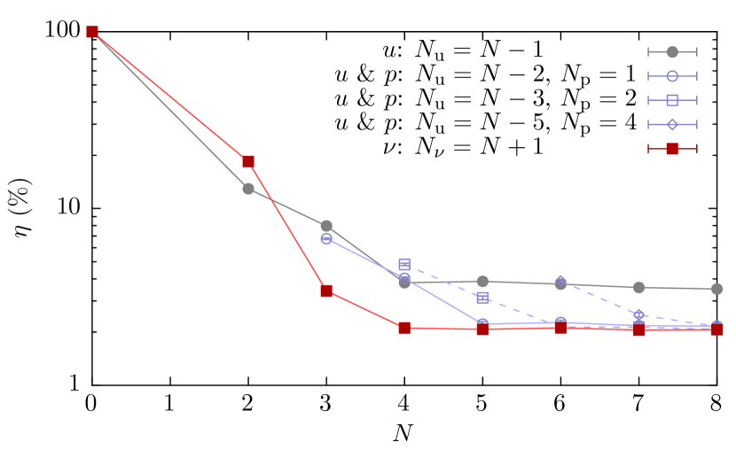
(a) Correlation energy missing

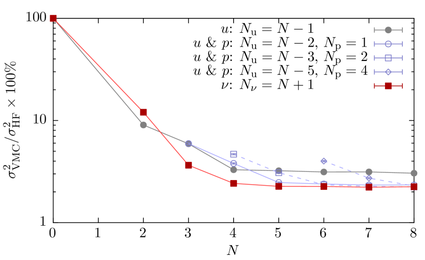
(b) Local energy variance

Figure 2: (Color online) (a) The percentage of the DMC correlation energy missing from VMC simulations of the homogeneous electron gas, with $N$ optimizable parameters in the Jastrow factor. Gray, blue, and red lines correspond to the $u$, $u$ & $p$, and $\nu$ term respectively. (b) The variance in the local energy when using different Jastrow factors, as a percentage of the variance in the local energy using the Hartree–Fock wavefunction. Error bars, where not visible, are smaller than the size of the points.

The $\nu$ Jastrow factor reproduces the best $u$ & $p$ accuracy of $\eta=2\%$ for $N\geq 4$. The need for only $N=4$ optimizable parameters as opposed to the $N\geq 5$ required for the $u$ & $p$ terms means the $\nu$ term is easier to optimize. Furthermore, the $\nu$ term has a single parameter $N_{\nu}$ that can be increased to improve accuracy, as opposed to having to choose both $N_{\mathrm{u}}$ and $N_{\mathrm{p}}$ for the $u$ & $p$ term, which reduces the size of the parameter space that needs to be explored.

The $\nu$ term has captured all of the correlation energy available to the $u$ & $p$ terms in this system, but another important quantity in QMC methods is the variance in the estimate of the energy. The variance of the local energy determines the efficiency of DMC simulations Foulkes01 ; Lee11 and also acts as a proxy for the quality of trial wavefunctions, as the variance in the local energy of the exact ground state is zero. In Fig. 2b we examine the variances in the local energy using the different Jastrow factors relative to the variance using the Hartree–Fock wavefunction. Again the $u$ term converges for $N\geq 4$, and the addition of $p$ terms reduces the variance by another 33% if a good choice of $N_{\mathrm{u}}$ and $N_{\mathrm{p}}$ is made with $N\geq 5$. The $\nu$ term achieves the same reduction in the variance in the local energy as these more complicated terms but with fewer optimizable parameters, $N\geq 4$.

The similar levels of the correlation energy captured by the $\nu$ and $u$ & $p$ terms may be understood in terms of the correlations described by these Jastrow factors. In Fig. 3 we show the $\nu$ and $N_{\mathrm{p}}=1$ $u$ & $p$ Jastrow functions with the $u$ Jastrow function subtracted, to allow us to focus on the long-range correlations. Both Jastrow functions capture non-trivial correlations in the corner of the simulation cell, outside the radius where the $u$ term is cut off to zero (shown by a gray arc), explaining their improved performance over the $u$ term. Furthermore, the correlations captured by the $\nu$ and $u$ & $p$ terms are very similar, confirming that both are able to be optimized to capture all of the available correlation energy. The similarity of the $\nu$ and $u$ & $p$ terms also ensures that the zero-wavevector limits of their Fourier transforms are likewise similar, and hence that the finite-size errors from the Jastrow factors are comparable and can be dealt with following the same prescription Chiesa06 ; Drummond08 .

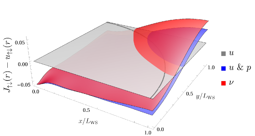
Figure 3: (Color online) The $N=5$ Jastrow functions with the $u$ Jastrow function subtracted, to show how the Jastrow functions vary at large inter-particle separation.

There is one further advantage to using the $\nu$ term in this system, rather than a $u$ & $p$ term. The $\nu$ term is a polynomial expansion, like the $u$ term, and this makes it quicker to evaluate than the $p$ term with its sinusoids from each element of the stars of reciprocal lattice vectors. For $N=5$, where both Jastrow factors have fully converged, the $N_{\mathrm{p}}=1$ $u$ & $p$ term in the Jastrow factor is 61% slower to evaluate than the $\nu$ term, and the $N_{\mathrm{p}}=2$ term takes over twice as long to evaluate as the $\nu$ term. This means that simulations with the $\nu$ term can be run significantly quicker than those with the $u$ & $p$ term, to obtain similar accuracy.

We have shown that the $\nu$ Jastrow factor captures the ground state energy of the HEG as well as a combination of the $u$ and $p$ terms, achieving the same accuracy and reduction in variance in the local energy. In addition to this, the $\nu$ term is easier to transfer between systems, as there is only one choice of parameter to make as opposed to two for the $u$ & $p$ term; the $\nu$ term requires $N=4$ linear optimizable parameters to converge, rather than $N=5$ non-linear parameters for the $u$ & $p$ term, making it cheaper to optimize; and the $\nu$ term is also quicker to evaluate. We now go on to test the $\nu$ Jastrow factor in an inhomogeneous periodic system, for which we take the example of crystalline beryllium.

IV Beryllium

To demonstrate that the advantages of the $\nu$ term are not restricted to simple homogeneous systems with cubic simulation cells, here we test it in a crystalline solid. As discussed in Section II.3, the $\nu$ term is constructed to interpolate between the symmetry of the interaction potential (purely radial) at short radius and the simulation cell symmetry at large separation. In order to demonstrate the generality of this construction, we will focus on an analysis of a crystal with relatively low symmetry, in the $\mathrm{P}6_{3}/\mathrm{mmc}$ (hexagonal) space group, where it is non-trivial to construct the long-range form of the $\nu$ term. The simplest example of a stable crystal with this space group at zero temperature, where QMC is applicable, is crystalline beryllium, and so we use that as our example system. At the end of this Section we will also discuss results in higher-symmetry face-centered cubic (FCC) and body-centered cubic (BCC) crystals.

We model crystalline beryllium using an hexagonal simulation cell containing 32 atoms. The Be²⁺ ions are represented by pseudopotentials Heine70 ; Pickett89 ; Drummond04 ; Needs10 , and the orbitals in the Slater determinants were obtained from a density functional theory Hohenberg64 ; Kohn65 (DFT) calculation using the castep code with a plane-wave basis set Payne92 ; Clark05 , converted to B-spline functions Hernandez97 ; Alfe04 .

The $u$ and $p$ terms are the same in this simulation cell as in the previous cubic case, with the $\mathbf{G}_{\ell}$ vectors for the $p$ term being the reciprocal lattice vectors of the simulation cell, organized into stars of equal-length vectors. In order to use the $\nu$ term we generalize its functional form to allow for the use of non-cuboidal simulation cells.

IV.1 Generalized form of $\nu$ term

To begin the generalization of the $\nu$ term we construct a set of vectors $\{\mathbf{B}\}$, formed of the reciprocal lattice vectors of the simulation cell and all symmetry-equivalent vectors. These vectors are exactly those normal to the faces of the conventional unit cell, and so encode the symmetry of the simulation cell, and have length such that $|\mathbf{B}_{i}\cdot\mathbf{r}_{\mathrm{face}}|=\pi$, for any vector $\mathbf{r}_{\mathrm{face}}$ lying in the corresponding conventional cell faces.

Constructing a matrix of the reciprocal lattice vectors $\{\mathbf{B}\}$ and then (left-)inverting and transposing it leads to a set of real-space vectors $\{\mathbf{A}\}$. By measuring the projection of the electron-electron separation vector $\mathbf{r}$ onto these real-space vectors we can express the electron-electron separation as $\mathbf{r}=\sum_{\zeta}\mathbf{A}_{\zeta}(\mathbf{B}_{\zeta}\cdot\mathbf{r})$. The inter-particle distance $r$ can then be expressed as

$$r =\sqrt{\left(\sum_{\zeta}\mathbf{A}_{\zeta}[\mathbf{B}_{\zeta}\cdot\mathbf{r}]\right)\cdot\left(\sum_{\xi}\mathbf{A}_{\xi}[\mathbf{B}_{\xi}\cdot\mathbf{r}]\right)}$$

$$=\sqrt{\sum_{i}\mathbf{A}_{i}\cdot\mathbf{A}_{i}w_{i}^{2}+2\sum_{j>k}\mathbf{A}_{j}\cdot\mathbf{A}_{k}w_{j}w_{k}},$$

where $w_{i}=\mathbf{B}_{i}\cdot\mathbf{r}$ expresses the projection of $\mathbf{r}$ onto $\mathbf{A}_{i}$ as a phase between $-\pi$ and $\pi$ as $\mathbf{r}$ runs between parallel faces of the conventional cell. In a directly analogous way to the previous, cuboidal form we then define the Jastrow function as

$$\nu_{\sigma\tau}(\mathbf{r})=\sum_{n=1}^{N_{\nu}}c_{n,\sigma\tau}\Big{|} \sum_{i}\mathbf{A}_{i}\cdot\mathbf{A}_{i}f^{2}(w_{i})+$$

$$2\sum_{j>k}\mathbf{A}_{j}\cdot\mathbf{A}_{k}g(w_{j})g(w_{k})\Big{|}^{n/2},$$ (5)

where in order to reduce to a radial expression at short radius we require that $f(w_{i})\to|w_{i}|$ and $g(w_{i})\to w_{i}$ as $\mathbf{r}\to\boldsymbol{0}$. In order to retain the symmetry of the simulation cell at large radii we demand $f(w_{i})$ be symmetric under $w_{i}\to-w_{i}$, whilst $g(w_{i})$ is required to be antisymmetric, and both functions should satisfy periodic boundary conditions at $|w_{i}|=\pi$. To satisfy these requirements we take $f$ and $g$ to have the simple forms

$$f(w_{i}) =|w_{i}|\left(1-\frac{|w_{i}/\pi|^{3}}{4}\right)$$

$$g(w_{i}) =w_{i}\left(1-\frac{3}{2}|w_{i}/\pi|+\frac{1}{2}|w_{i}/\pi|^{2}\right).$$ (6)

$f(w_{i})$ is very similar to the cuboidal form given in Eq. (4), and if we use a cuboidal simulation cell with orthogonal lattice vectors, where $\{\mathbf{A}\}=\{\mathbf{a}_{1}/2\pi,\mathbf{a}_{2}/2\pi,\mathbf{a}_{3}/2\pi\}$ and $\{\mathbf{B}\}=\{\mathbf{b}_{1},\mathbf{b}_{2},\mathbf{b}_{3}\}$, the general form of the Jastrow function Eq. (5) reduces to the cuboidal form Eq. (4). $g(w_{i})$ is the lowest-order polynomial-like expansion that is antisymmetric under $w_{i}\to-w_{i}$. The sets of vectors $\{\mathbf{A}\}$ and $\{\mathbf{B}\}$ that we use for the hexagonal simulation cell, as well as for other common simulation cell geometries, are given in the Appendix.

IV.2 Electron-ion correlations

In crystalline systems there are correlations between the ions and electrons, as well as those between electrons. The DFT orbitals in the Slater determinants describe most of the electron-ion correlations, but these are modified by the introduction of electron-electron correlations in the Jastrow factor: in our simulations we add optimizable electron-ion correlations to the electron-electron Jastrow factor to counter this,

$$J(\mathbf{R})=\sum_{\begin{subarray}{c}j>i\\ \sigma,\tau\in\{\uparrow,\downarrow\}\end{subarray}}J_{\sigma\tau}(\mathbf{r}_{ij})+\sum_{\begin{subarray}{c}i,I\\ \sigma\in\{\uparrow,\downarrow\}\end{subarray}}\chi_{\sigma}(\mathbf{r}_{iI}),$$

where $\mathbf{r}_{iI}=\mathbf{r}_{i}-\mathbf{r}_{I}$, for ion positions $\mathbf{r}_{I}$, $i$ running over all electrons, and $I$ running over all ions. It has been shown Drummond04 ; Rios12 that a short-ranged $u$-like expansion in electron-ion separation,

$$\chi_{\sigma}(\mathbf{r}_{iI})= \left(\frac{L^{\chi}_{\sigma}}{3}\beta_{1,\sigma}+\sum_{m=1}^{N_{\chi}}\beta_{m,\sigma}r_{iI}^{m}\right)\times$$

$$\times\left(1-r_{iI}/L^{\chi}_{\sigma}\right)^{3}\Theta(L^{\chi}_{\sigma}-r_{iI}),$$

captures the most important electron-ion correlations in the electron-ion term, without the need for a longer-ranged $p$-like term. The cutoff length $L^{\chi}_{\sigma}$ is generally comparable to the inter-ionic distance, and we use $N_{\chi}=4$ in our simulations. As we use pseudopotentials for the ions there is no gradient discontinuity in the wavefunction at electron-ion coincidence. We also tested a cuspless form of the $\nu$ Jastrow function to capture the electron-ion correlations, which agreed with the energies obtained using $\chi_{\sigma}(\mathbf{r}_{iI})$ to within $10^{-5}$ a.u. with the same number of variational parameters. This confirms that it is the short-range electron-ion correlations that are the most important to capture, and so we shall use the well-established $\chi_{\sigma}(\mathbf{r}_{iI})$ term in the following investigations.

In all-electron QMC simulations, particularly of molecules, the addition of three-body electron-electron-ion correlations to the Jastrow factor lowers the calculated energy Foulkes01 ; Rios12 ; Huang97 , as these terms allow a more detailed description of tightly-bound electrons. However, electron-electron-ion correlations are less important in simulations using pseudopotentials, and including them here changes the correlation energy by less than 0.9%. Similarly to the electron-ion term the dominant effect of electron-electron-ion terms is at short radius, and so the $\nu$ Jastrow factor formalism is expected to offer limited improvements relative to an isotropic $u$-like term in constructing such terms. As electron-electron-ion terms make a small difference to the energy and will not help us to discrimitate between the $u$, $u$ & $p$, and $\nu$ terms we neglect them here, although they should of course be included in simulations targeting high accuracy.

The full Jastrow function is then obtained by combining the electron-ion term $\chi_{\sigma}(\mathbf{r}_{iI})$ with the electron-electron Jastrow functions under examination, the $u$, $u$ & $p$, and generalized $\nu$ terms. We now examine the accuracy and efficiency of these Jastrow functions for simulating crystalline beryllium.

IV.3 Results

(a) Correlation energy missing

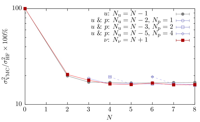
(b) Local energy variance

Figure 4: (Color online) (a) The percentage of the DMC correlation energy missing from VMC simulations of crystalline beryllium, with $N$ optimizable parameters in the Jastrow factor. Gray, blue, and red lines correspond to the $u$, $u$ & $p$, and $\nu$ term respectively. (b) The variance in the local energy when using different Jastrow factors, as a percentage of the variance in the local energy using the Hartree–Fock wavefunction. Error bars, where not visible, are smaller than the size of the points.

In Fig. 4a we compare the percentages of the DMC correlation energy missing, $\eta$, when the various Jastrow factors are used with $N$ variational parameters in the electron-electron Jastrow factor. We observe that a $u$ term alone is always missing nearly 20% of the correlation energy, and moreover that the addition of a single $p$ term does not significantly improve the result. This is in contrast to the case of the HEG, where the addition of a single $p$ term was the most important step in achieving a high-accuracy $u$ & $p$ term. This is due to the fact that, in the beryllium simulation cell, the $\mathbf{b}_{3}$ lattice vector orthogonal to the hexagonal planes is shorter than those in the $\mathbf{b}_{1},~{}\mathbf{b}_{2}$ plane, and so the first $p$ term only acts along the $c$ axis, not providing flexibility to capture correlations in the hexagonal planes. However, the addition of just one more $p$ term reduces the correlation energy missing to around 9%, and the addition of more $p$ terms to this does not significantly alter the result. This means that to achieve convergence we again require $N=5$ when using the $u$ & $p$ term.

As in the HEG, the $\nu$ term achieves comparable accuracy to the most accurate $u$ & $p$ terms, reaching convergence by $N=2$. This, combined with the necessity of otherwise using $N\geq 5$ for the $u$ and $p$ term, of which $N_{\mathrm{p}}=2$ are expensive $p$ terms, means that the $\nu$ term is significantly cheaper to optimize and use than alternative Jastrow factors.

In Fig. 4b we examine the variance in the local energy using different Jastrow factors. There is significantly less difference here between the Jastrow factors than in the proportion of the correlation energy they capture, but the $\nu$ term again performs as well as the most detailed other Jastrow factors, meaning that the trial wavefunctions have similar efficiency in DMC.

Crystal type (example system)	$\nu$	$u$ & $p$: $N_{\mathrm{p}}=2$
Hexagonal (Be)	$8.6(1)\%$	$9.3(1)\%$
BCC (Li)	$4.7(1)\%$	$5.0(1)\%$
FCC (Si)	$10.1(2)\%$	$9.6(2)\%$

Table 1: The percentage of the DMC correlation energy missing within VMC, $\eta$, for the $\nu$ and $u$ & $p$ terms with $N=5$ in example systems: crystalline beryllium in a hexagonal simulation cell; crystalline lithium in a body-centered cubic (BCC) simulation cell; and crystalline silicon in a face-centered cubic (FCC) simulation cell. Bracketed numbers indicate the standard error in the values for $\eta$.

As well as hexagonal crystalline beryllium, we have also tested the electron-electron $\nu$ term in other crystals with different symmetry. The missing correlation energy when using the $\nu$ term and the $N_{\mathrm{p}}=2$ $u$ & $p$ term is shown in Table 1. The $u$ & $p$ term is not significantly improved by increasing $N_{\mathrm{p}}$ in any of these crystals, and we use $N=5$ as this is where the $u$ & $p$ term approaches its converged accuracy; in each case the $\nu$ term is already converged.

The two Jastrow factors capture similar levels of the correlation energy in each system, indicating that the $\nu$ term is a good general choice of Jastrow factor for use in crystalline systems, with the slight differences between the $\nu$ and $u$ & $p$ terms in different systems being due to the exact details of the symmetry of the simulation cell in each case, some of which are better captured by the $\nu$ term than others. However, overall the differences between Jastrow factors are smaller than the differences between systems, and the $\nu$ Jastrow factor achieves high accuracy whilst having fewer (and only linear) parameters to optimize and being cheaper to evaluate, due to being polynomial as opposed to sinusoidal.

V Discussion

We have proposed and tested a form of electron-electron Jastrow factor that interpolates between the radial symmetry of the Coulomb potential at short range and the space-group symmetry of the simulation cell at large separation. The $\nu$ Jastrow factor captures comparable levels of the correlation energy to the most detailed $u$ & $p$ terms used in the literature, and converges with fewer variational parameters. There is also only one choice of input to the $\nu$ term, the expansion order $N_{\nu}$, which reduces the parameter space to be explored compared to the two variables, $N_{\mathrm{u}}$ and $N_{\mathrm{p}}$, required for the $u$ & $p$ term. Finally, the polynomial $\nu$ term is quicker to evaluate than the plane-wave $p$ term.

It would be possible to apply the ideas behind the $\nu$ term to higher angular-momentum terms in a Jastrow factor: for instance, carrying out the transformation $x/r\to g(x)/\sqrt{f^{2}(x)+f^{2}(y)+f^{2}(z)}$ would allow the $Y_{11}$ spherical harmonic to be expressed in a way that satisfies the symmetry of a cuboidal simulation cell. The $\nu$ term could also be used in systems with interactions other than the Coulomb potential; for instance, QMC may also be used to study the dipolar Whitehead16 and contact Whitehead16a interactions in cold atomic gases, and also more exotic interactions such as those found in 2D semiconductors Ganchev15 . The interpolation between symmetries of the $\nu$ term could also be applicable more widely than just in Jastrow factors. Any expansion in or use of inter-particle separation in a numerical investigation could be written instead in terms of the $f$ and $g$ functions of the $\nu$ term, and so would immediately satisfy periodic boundary conditions in the simulation cell. Systems that might be well-suited to this approach could include two-particle pairing orbitals in Slater determinants Bouchaud88 , large-amplitude phonons simulated within density functional theory Baroni01 , or the construction of force fields that natively reflect bond angles for molecular dynamics simulations Mackerell04 .

The $\nu$ Jastrow factor is implemented in the casino QMC package Needs10 ; casino . Data used for this paper are available online repository .

*

Appendix A Symmetry-related vectors for the $\nu$ term

Here we enumerate the $\{\mathbf{A}\}$ and $\{\mathbf{B}\}$ vectors for use in the $\nu$ term for some common simulation-cell geometries.

A.1 Cubic cell

For a cubic cell with lattice vectors $\mathbf{a}_{1}=a[100]$, $\mathbf{a}_{2}=a[010]$, $\mathbf{a}_{3}=a[001]$, the symmetry-related vectors take the form

$$\{\mathbf{A}\} =\frac{1}{2\pi}\{\mathbf{a}_{1},\mathbf{a}_{2},\mathbf{a}_{3}\}$$

$$\{\mathbf{B}\} =\{\mathbf{b}_{1},\mathbf{b}_{2},\mathbf{b}_{3}\}.$$

A.2 FCC cell

For a face-centered cubic cell with lattice vectors $\mathbf{a}_{1}=\frac{a}{2}[011]$, $\mathbf{a}_{2}=\frac{a}{2}[101]$, $\mathbf{a}_{3}=\frac{a}{2}[110]$, the symmetry-related vectors take the form

$$\{\mathbf{A}\} =\frac{1}{8\pi}\{3\mathbf{a}_{1}-\mathbf{a}_{2}-\mathbf{a}_{3},3\mathbf{a}_{2}-\mathbf{a}_{3}-\mathbf{a}_{1},$$

$$\qquad\quad\,3\mathbf{a}_{3}-\mathbf{a}_{1}-\mathbf{a}_{2},\mathbf{a}_{1}+\mathbf{a}_{2}+\mathbf{a}_{3}\}$$

$$\{\mathbf{B}\} =\{\mathbf{b}_{1},\mathbf{b}_{2},\mathbf{b}_{3},\mathbf{b}_{1}+\mathbf{b}_{2}+\mathbf{b}_{3}\}.$$

A.3 BCC cell

For a body-centered cubic cell with lattice vectors $\mathbf{a}_{1}=\frac{a}{2}[\bar{1}11]$, $\mathbf{a}_{2}=\frac{a}{2}[1\bar{1}1]$, $\mathbf{a}_{3}=\frac{a}{2}[11\bar{1}]$, the symmetry-related vectors take the form

$$\{\mathbf{A}\} =\frac{1}{8\pi}\{2\mathbf{a}_{1}+\mathbf{a}_{2}+\mathbf{a}_{3},2\mathbf{a}_{2}+\mathbf{a}_{3}+\mathbf{a}_{1},$$

$$\qquad\quad\,2\mathbf{a}_{3}+\mathbf{a}_{1}+\mathbf{a}_{2},\mathbf{a}_{1}-\mathbf{a}_{2},\mathbf{a}_{1}-\mathbf{a}_{3},\mathbf{a}_{2}-\mathbf{a}_{3}\}$$

$$\{\mathbf{B}\} =\{\mathbf{b}_{1},\mathbf{b}_{2},\mathbf{b}_{3},\mathbf{b}_{1}-\mathbf{b}_{2},\mathbf{b}_{1}-\mathbf{b}_{3},\mathbf{b}_{2}-\mathbf{b}_{3}\}.$$

A.4 Hexagonal cell

For a hexagonal cell with lattice vectors $\mathbf{a}_{1}=a[100]$, $\mathbf{a}_{2}=a[\frac{1}{2}\frac{\sqrt{3}}{2}0]$, $\mathbf{a}_{3}=c[001]$, the symmetry-related vectors take the form

$$\{\mathbf{A}\} =\frac{1}{6\pi}\{2\mathbf{a}_{1}-\mathbf{a}_{2},2\mathbf{a}_{2}-\mathbf{a}_{1},3\mathbf{a}_{3},\mathbf{a}_{1}+\mathbf{a}_{2}\}$$

$$\{\mathbf{B}\} =\{\mathbf{b}_{1},\mathbf{b}_{2},\mathbf{b}_{3},\mathbf{b}_{1}+\mathbf{b}_{2}\}.$$

References

- (1) W.M.C. Foulkes, L. Mitas, R.J. Needs, and G. Rajagopal, Rev. Mod. Phys. 73, 33 (2001).
- (2) P.J. Reynolds, D.M. Ceperley, B.J. Alder, and W.A. Lester Jr., J. Chem. Phys. 77, 5593 (1982).
- (3) R.J. Jastrow, Phys. Rev. 98, 1479 (1955).
- (4) A.J. Williamson, S.D. Kenny, G. Rajagopal, A.J. James, R.J. Needs, L.M. Fraser, W.M.C. Foulkes, and P. Maccallum, Phys. Rev. B 53, 9640 (1996).
- (5) N.D. Drummond, M.D. Towler, and R.J. Needs, Phys. Rev. B 70, 235119 (2004).
- (6) P. López Ríos, P. Seth, N.D. Drummond, and R.J. Needs, Phys. Rev. E 86, 036703 (2012).
- (7) G. Ortiz and P. Ballone, Phys. Rev. B 50, 1391 (1994).
- (8) W.L. McMillan, Phys. Rev. 138, A442 (1965).
- (9) D.M. Ceperley, Phys. Rev. B 18, 3126 (1978).
- (10) A.D. Güçlü, Gun Sang Jeon, C.J. Umrigar, and J.K. Jain, Phys. Rev. B, 72, 205327 (2005).
- (11) G.E. Astrakharchik, J. Boronat, I.L. Kurbakov, and Yu.E. Lozovik, Phys. Rev. Lett. 98, 060405 (2007).
- (12) J.B. Anderson, J. Chem. Phys. 65, 4121 (1976).
- (13) R.J. Needs, M.D. Towler, N.D. Drummond, and P. López Ríos, J. Phys.: Condensed Matter 22, 023201 (2010).
- (14) C.J. Umrigar, K.G. Wilson, and J.W. Wilkins, Phys. Rev. Lett. 60, 1719 (1988).
- (15) T. Kato, Commun. Pure Appl. Math. 10, 151 (1957).
- (16) Y.S. Al-Hamdani, D. Alfè, O.A. von Lilienfeld, and A. Michaelides, J. Chem. Phys. 141 18C530 (2014).
- (17) J. Chen, X. Ren, X.-Z. Li, D. Alfè, and E. Wang, J. Chem. Phys. 141, 024501 (2014).
- (18) M.J. Gillan, D. Alfè, and F.R. Manby, J. Chem. Phys. 143, 102812 (2015).
- (19) J.H. Lloyd-Williams, R.J. Needs, and G.J. Conduit, Phys. Rev. B 92, 075106 (2015).
- (20) G.J. Conduit, A.G. Green, and B.D. Simons, Phys. Rev. Lett. 103, 207201 (2009).
- (21) N.D. Drummond and R.J. Needs, Phys. Rev. B 87, 045131 (2013).
- (22) T.M. Whitehead and G.J. Conduit, Phys. Rev. A 93, 022706 (2016).
- (23) S. Chiesa, D.M. Ceperley, R.M. Martin, and M. Holzmann, Phys. Rev. Lett. 97, 076404 (2006).
- (24) G.G. Spink, R.J. Needs, and N.D. Drummond, Phys. Rev. B 88, 085121 (2013).
- (25) C.W. von Keyserlingk and G.J. Conduit, Phys. Rev. B 87, 184424 (2013).
- (26) R. Maezono, N.D. Drummond, A. Ma, and R.J. Needs, Phys. Rev. B 82, 184108 (2010).
- (27) E. Mostaani, N.D. Drummond, and V.I. Fal’ko, Phys. Rev. Lett. 115, 115501 (2015).
- (28) N.D. Drummond and R.J. Needs, Phys. Rev. B 72, 085124 (2005).
- (29) D.M. Ceperley and B.J. Alder, Phys. Rev. Lett. 45, 566 (1980).
- (30) F.H. Zong, C. Lin, and D.M. Ceperley, Phys. Rev. E 66, 036703 (2002).
- (31) N.D. Drummond, Z. Radnai, J.R. Trail, M.D. Towler, and R.J. Needs, Phys. Rev. B 69, 085116 (2004).
- (32) P.R.C. Kent, R.J. Needs, and G. Rajagopal, Phys. Rev. B 59, 12344 (1999).
- (33) C.J. Umrigar, J. Toulouse, C. Filippi, S. Sorella, and R.G. Hennig, Phys. Rev. Lett. 98, 110201 (2007).
- (34) R.M. Lee, G.J. Conduit, N. Nemec, P. López Ríos, and N.D. Drummond, Phys. Rev. E 83, 066706 (2011).
- (35) N.D. Drummond, R.J. Needs, A. Sorouri, and W.M.C. Foulkes, Phys. Rev. B 78, 125106 (2008).
- (36) V. Heine, Solid State Physics 24, 1 (1970).
- (37) W.E. Pickett, Computer Physics Reports, 9, 115 (1989).
- (38) P. Hohenberg and W. Kohn, Phys. Rev. 136, B864 (1964).
- (39) W. Kohn and L.J. Sham, Phys. Rev. 140, A1133 (1965).
- (40) M.C. Payne, M.P. Teter, D.C. Allan, T.A. Arias, and J.D. Joannopoulos, Rev. Mod. Phys. 64, 1045 (1992).
- (41) S.J. Clark, M.D. Segall, C.J. Pickard, P.J. Hasnip, M.J. Probert, K. Refson, and M.C. Payne, Z. Kristall 220, 567 (2005).
- (42) E. Hernández, M.J. Gillan, and C.M. Goringe, Phys. Rev. B 55, 13485 (1997).
- (43) D. Alfè and M.J. Gillan, Phys. Rev. B 70, 161101(R) (2004).
- (44) C.-J. Huang, C.J. Umrigar, M.P. Nightingale, J. Chem. Phys. 107, 3007 (1997).
- (45) T.M. Whitehead, L.M. Schonenberg, N. Kongsuwan, R.J. Needs, and G.J. Conduit, Phys. Rev. A 93, 042702 (2016).
- (46) B. Ganchev, N.D. Drummond, I. Aleiner, and V. Fal’ko, Phys. Rev. Lett. 114, 107401 (2015).
- (47) J.P. Bouchaud, A. Georges, and C. Lhuillier, J. Physique 49, 553 (1988).
- (48) S. Baroni, S. de Gironcoli, A. Dal Corso, and P. Giannozzi, Rev. Mod. Phys. 73, 515 (2001).
- (49) A.D. Mackerell, J. Comput. Chem. 25, 1584 (2004).
- (50) Available from https://vallico.net/casinoqmc/.
- (51) T.M. Whitehead, M.H. Michael, and G.J. Conduit, Cambridge University DSpace repository, http://dx.doi.org/10.17863/CAM.694.