Neutrino Flavor Evolution in Binary Neutron Star Merger Remnants

Abstract

We study the neutrino flavor evolution in the neutrino-driven wind from a binary neutron star merger remnant consisting of a massive neutron star surrounded by an accretion disk. With the neutrino emission characteristics and the hydrodynamical profile of the remnant consistently extracted from a three-dimensional simulation, we compute the flavor evolution by taking into account neutrino coherent forward scattering off ordinary matter and neutrinos themselves. We employ a “single-trajectory” approach to investigate the dependence of the flavor evolution on the neutrino emission location and angle. We also show that the flavor conversion in the merger remnant can affect the (anti-)neutrino absorption rates on free nucleons and may thus impact the $r$-process nucleosynthesis in the wind. We discuss the sensitivity of such results on the change of neutrino emission characteristics, also from different neutron star merger simulations.

I Introduction

The first gravitational wave signal detection from a binary black hole merger observed by the Virgo-LIGO collaboration has opened the era of gravitational wave astronomy Abbott et al. (2016). Since binary neutron star (BNS) mergers Rosswog (2015); Faber and Rasio (2012) are one of the major sources of gravitational waves, a measurement of such a signal is anticipated. Moreover, BNS mergers are considered as the likely production site for rapid neutron capture (r-process) nucleosynthesis Lattimer and Schramm (1974); Eichler et al. (1989) and as a potential source of short gamma-ray bursts Paczynski (1986); Eichler et al. (1989); Nakar (2007).

Similar to core-collapse supernovae, the dynamics of such astrophysical environments is expected to be affected by neutrinos. A significant amount of energy is carried by them and their interaction with matter affects the neutron-to-proton ratio (or equivalently, the electron fraction $Y_{e}$), which is a crucial elements for nucleosynthesis. Since the main processes of transporting energy and altering the composition are neutrino flavor-dependent, any mechanism that changes the flavor content of neutrinos should be studied in order to fully access their role in these environments.

Since the first proposals of neutrino oscillations by the pioneering works of Pontecorvo Pontecorvo (1957, 1958, 1968), it took almost half a century before neutrino flavor oscillations were finally discovered by the Super-Kamiokande collaboration Fukuda et al. (1998) and the Sudbury Neutrino Observatory Ahmad et al. (2002). It was early recognized that if neutrinos are on their way through a dense background medium, they acquire a refractive index due to coherent forward scattering with the background particles Wolfenstein (1978). This can possibly lead to flavor conversions, like in the Sun, where the Mikheyev-Smirnov-Wolfenstein (MSW) effect Wolfenstein (1978); Mikheyev and Smirnov (1986) takes place. Furthermore, neutrinos themselves can constitute a significant background. This occurs in the early universe and in astrophysical environments, such as core-collapse supernovae, BNS mergers, and collapsars, where large neutrino fluxes are present so that their number density are comparable to or larger than that of matter. In these environments, the neutrino coherent forward scattering off neutrinos produces flavor-diagonal Fuller et al. (1987); Nötzold and Georg (1988) as well as off-diagonal contributions to the neutrino refractive index matrix, as realized by Pantaleone Pantaleone (1992a, b). The neutrino self-interaction contribution couples their flavor evolution non-linearly and causes collective oscillations where different types of collective phenomena (synchronized and bipolar oscillations, spectral splits/swaps) can arise (see Chakraborty et al. (2016); Duan (2015); Duan et al. (2010) and references therein).

In environments with a disk geometry (e.g., in collapsars or BNS mergers) another effect associated with neutrino self-interactions was revealed through numerical calculations Malkus et al. (2012, 2014, 2016): If the matter and neutrino self-interaction potentials almost cancel each other, matter-neutrino resonances (MNR) can occur and cause flavor conversion in regions above the emitting disk. Different from the case of a deleptonizing proto-neutron star, the material in a binary neutron star merger starts with a huge neutron excess. The prevailing temperatures of the remnant (several $\mathrm{MeV}$ Rosswog (2015)) allow positron captures on neutrons ($n+e^{+}\to p+\bar{\nu}_{e}$) to increase the electron fraction and to release more electron antineutrinos than electron neutrinos. Initially, this larger number flux of electron antineutrinos causes a different sign in the neutrino self-interaction potential compared to the neutrino-matter potential. Depending on the matter profile, this can allow an almost cancellation of the two potentials at some point. As neutrinos leave the emission surface, the role of geometry becomes more important Malkus et al. (2016): Since the electron antineutrinos decouple deeper inside the remnant than electron neutrinos, the latter have a larger emission surface. In the neutrino self-interaction potential this difference in geometry can induce a flip of sign at some point and can allow for symmetric MNR Malkus et al. (2016), as first found in the context of collapsar-type disks Malkus et al. (2012). In Malkus et al. (2014) another type of MNR, later called standard MNR Malkus et al. (2016), where the neutrino self-interaction potential does not change its sign, was found. In Malkus et al. (2016), both the standard and the symmetric MNR were investigated within models with equal and different disk sizes for each neutrino species. In addition, for the symmetric MNR, the possible impact on disk wind nucleosynthesis was investigated and it was found that it could potentially favor the formation of r-process elements Malkus et al. (2012, 2016).

The investigation of this phenomenon in schematic models shows that the underlying mechanism can be understood in terms of adiabatic solutions similar to the MSW flavor transformation Wu et al. (2016a); Väänänen and McLaughlin (2016). It should be mentioned that the MNR shares common features with the non-linear feedback in conjunction with helicity transformations Vlasenko et al. (2014a). Furthermore, we note that the occurence of the MNR is not restricted to disk scenarios. Since different signs in the matter and neutrino potentials are necessary, this effect could potentially occur in other environments, too. For example in core collapse supernovae by incorporating active-sterile neutrino mixing Wu et al. (2016b) or non-standard neutrino interactions Stapleford et al. (2016).

Due to the non-linear nature of the problem and the anisotropic astrophysical environments, numerically solving flavor evolution problems including neutrino self-interactions requires some assumptions. As will be discussed in detail, one typically assumes that the initial symmetry of the system is maintained. Within this assumption, the flavor evolution of neutrinos in a spherically symmetric environment becomes solvable in the so-called “bulb-model” Duan et al. (2006). This approach is usually called “multi-angle approximation” when the radial coordinate and the angular variable are retained to specify the neutrino propagation. In contrast, “single-angle approximation”, which was also often used in studying such problems, further assumes that the flavor evolution of neutrinos only depends on the radial coordinate Qian and Fuller (1995). It was found that in the context of supernovae, the solutions of single-angle and multi-angle approximations can be similar (e.g., Duan et al. (2006); Fogli et al. (2007)) but sometimes different (e.g., Dasgupta et al. (2009); Duan and Friedland (2011)). Note that based on the “bulb-model”, it was shown that, the matter potential can induce kinematical decoherence, suppress flavor conversion, or the flavor instability could be shifted compared to the single-angle case when performing a multi-angle treatment Duan et al. (2006).

In a system with a disk-like geometry, however, the problem is intrinsically different from a spherically symmetric one as the disk itself defines a particular direction with the disk center. In this case, one naturally expects that the flavor evolution history of neutrinos emitted from different parts of the disk with different emission angles should be different. In the first flavor evolution works with a disk geometry Malkus et al. (2012, 2014, 2016) neutrinos were followed on $45^{\circ}$-trajectories from accretion disks around black holes. The disk model parameters were chosen to be consistent with studies of the collapse of rotating massive stars Malkus et al. (2012) or the mergers of a black hole and a neutron star Malkus et al. (2014, 2016).

In this work, we study the trajectory dependence of the neutrino flavor evolution in the neutrino-driven wind from a binary neutron star merger remnant before black hole formation. To explore the dependence of flavor evolution on the neutrino emission location and angles, we use a “single-trajectory” approximation which assumes that at every point of a given neutrino trajectory, the flavor states of all neutrinos with the same energy identically contribute to the self-interaction. To this aim we use results from the detailed simulations of Perego et al. (2014), in particular, matter profiles (density, electron fraction and temperature), neutrino luminosities, and mean neutrino energies. We present numerical results on the flux-averaged neutrino and antineutrino probabilities for several trajectories where neutrino self-interaction and matter potentials differ. We then discuss the potential impact on nucleosynthesis by showing the change in the (anti-)neutrino capture rates on free nucleons, relevant for $r$-process nucleosynthesis, due to flavor evolution along these trajectories. We also investigate the sensitivity of the flavor evolution to different emission characteristics within the same model, or considering uncertainties from available simulations.

The paper is organized as follows. In Sec. II, we explain the procedure to determine the neutrino emission surfaces. In Sec. III, we discuss the equations of motion governing the neutrino flavor evolution and the method we adopted in this work to investigate the trajectory dependence. In Sec. IV, we describe the unoscillated potentials along chosen trajectories. In Sec. V, we present our numerical results of the trajectory dependence and the impact on the capture rates. We comment on the dependence of the results on the initial emission parameters. We discuss the implications and conclude in Sec. VI. If not otherwise stated, we employ natural units: $\hbar\equiv c\equiv k_{\mathrm{B}}\equiv 1$.

II Disk structure and neutrino surfaces in binary neutron star merger remnants

II.1 BNS merger remnant

Our discussion is based on a long-term three-dimensional Newtonian hydrodynamics simulation of the neutrino-driven wind that emerges from the remnant of the merger of two non-spinning $1.4\,M_{\odot}$ neutron stars Perego et al. (2014). As a result of the merging process, a massive neutron star (MNS) forms in the central region, surrounded by an accretion disk. The MNS has a rest mass possibly larger then the maximally allowed rest mass of a non-rotating neutron star Hotokezaka et al. (2013). In the case of a gravitational unstable object, its temporary stability against gravitational collapse is expected to be provided primarily by differential rotation Baumgarte et al. (2000), but also other mechanisms, like thermal pressure, could give additional support Baumgarte et al. (2000); Kaplan et al. (2014). For this reason, the MNS is assumed to stay stable during the simulation time, $\sim\mathcal{O}(100)$ ms after the merger, and is treated as a stationary rotating object.

Typical timescales of the disk are given by the dynamical timescale $t_{\mathrm{dyn}}^{\mathrm{disk}}\sim\mathcal{O}(10)$ ms and the much longer viscous timescale $t_{\mathrm{visc}}^{\mathrm{disk}}\sim\mathcal{O}(300)$ ms which gives an estimate of the lifetime of the disk Perego et al. (2014). The latter is characterized by a typical radius $R_{\mathrm{disk}}\sim\mathcal{O}(100)$ km and innermost density $\rho_{\mathrm{disk}}\sim 5\times 10^{11}\mathrm{g}\,\mathrm{cm}^{-3}$, while the central density of the MNS is a few $10^{14}\,\mathrm{g}\,\mathrm{cm}^{-3}$ as can be inferred from Fig. 1, where we plot the density at $100\,\mathrm{ms}$ after the merger. Due to the high densities of the remnant, neutrinos act as the major cooling source and other particles are essentially trapped on the relevant timescales.

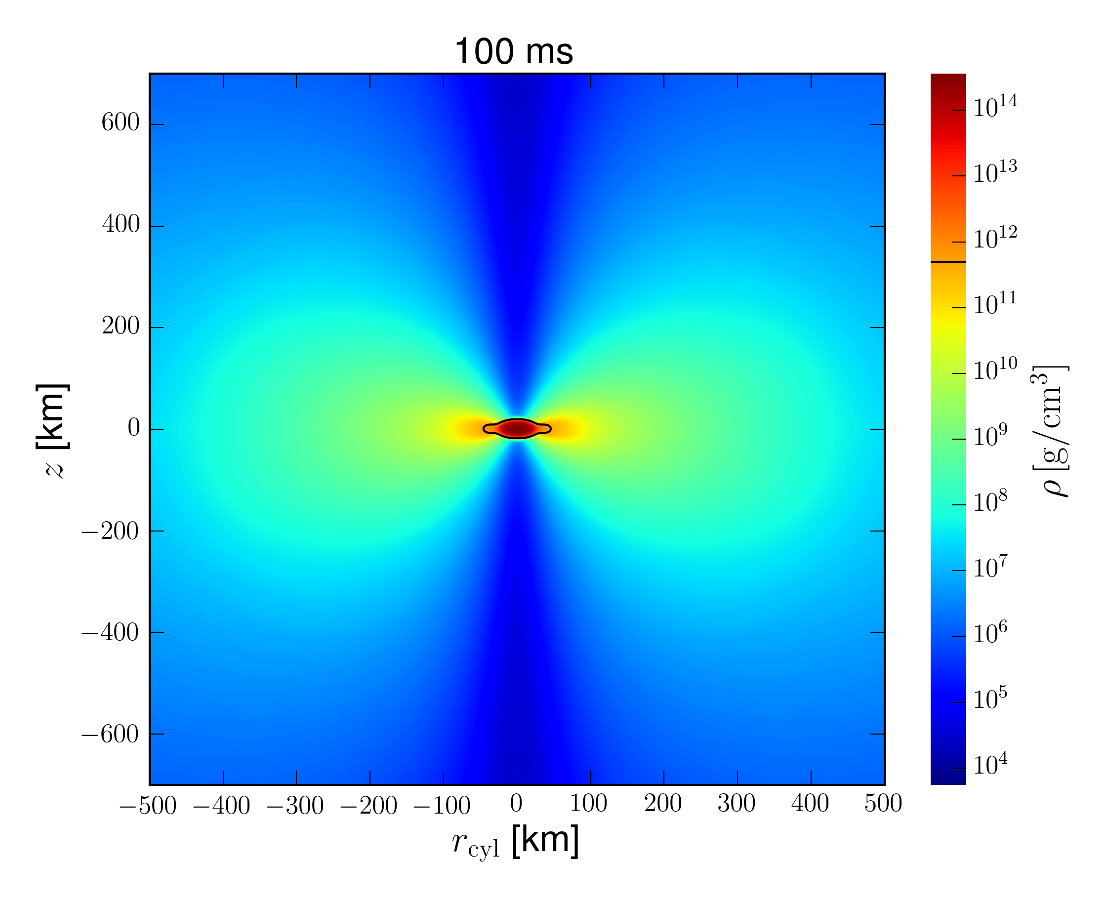
Figure 1: Density profile as a function of cylindrical coordinates $z$ and $r_{\mathrm{cyl}}$ at $t=100\,\mathrm{ms}$ after the merger. The contour $\rho\approx 5\times 10^{11}\,\mathrm{g}/\mathrm{cm}^{3}$ delimits the innermost part of the disk that is comparable to the surface density of a proto-neutron star Perego et al. (2014).

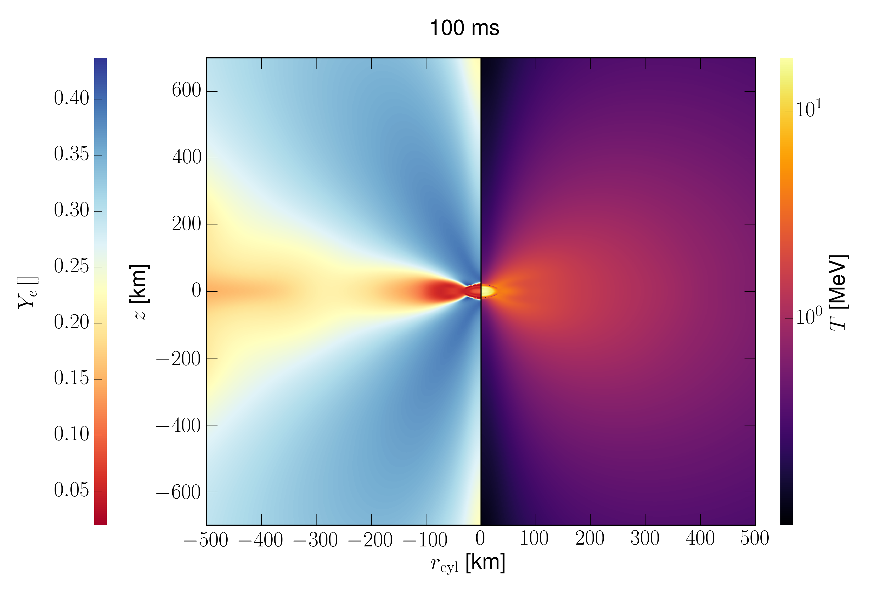
Figure 2: Electron fraction (left panel) and matter temperature (right panel) as functions of cylindrical coordinates $z$ and $r_{\mathrm{cyl}}$ at $t=100\,\mathrm{ms}$ after the merger.

We consider the emission and the absorption of neutrinos from the MNS and the surrounding disk Perego et al. (2016). Similar to the case of a proto-neutron star, those neutrinos can cause a mass outflow, called neutrino-driven wind, by energy deposition via absorption and scattering processes Duncan et al. (1986); Qian and Woosley (1996). This wind, together with viscously-driven ejecta, is blown away mainly from the disk Just et al. (2015); Metzger and Fernández (2014); Perego et al. (2014); Dessart et al. (2009); Surman et al. (2008). Since the rotational period of the accretion disk and of the MNS is much smaller than the neutrino diffusion timescale and the disk lifetime, after a few orbits the remnant approaches a quasi-axisymmetric configuration. Thus, we assume rotational symmetry around the MNS rotational axis and use the axisymmetric averages of hydrodynamical quantities (matter density, temperature and electron fraction) from the simulation Perego et al. (2014) for our calculations below. These quantities are shown in Figs. 1 and 2. Local deviations of the three-dimensional quantities with respect to the cylindrically averaged values are usually $\lesssim\,15\%$ inside the densest part of the remnant.

II.2 Neutrino surfaces

In this Sec., we construct a neutrino emission disk from the simulation result described in Sec. II.1. We first determine the neutrino emission surface by calculating the neutrino opacity in the remnant. The reactions giving the most relevant contributions to the optical depth are listed in Table 1. For their corresponding cross sections $\sigma$ we use the expressions described in Burrows et al. (2006) without weak magnetism corrections (see Appendix A).

Table 1: Neutrino reactions considered in our model, where $N\in\{n,p\}$. For reaction (i), $\nu$ refers to all neutrino species. In the second column we denote the associated mean free paths, where (sc) refers to scattering while (ab) to absorption. The corresponding cross sections are taken from Burrows et al. (2006).

	Reaction	Inverse mean free path
(i)	$\nu+N\rightarrow\nu+N$	$\lambda_{\nu N,\mathrm{sc}}^{-1}$
(ii)	$\nu_{e}+n\rightarrow e^{-}+p$	$\lambda_{\nu_{e},\mathrm{ab}}^{-1}$
(iii)	$\bar{\nu}_{e}+p\rightarrow e^{+}+n$	$\lambda_{\bar{\nu}_{e},\mathrm{ab}}^{-1}$

One main contribution to the opacity for all neutrino species is due to elastic neutrino scattering off free nucleons ($N=n,p$). Due to the presence of neutron-rich matter, the absorption of $\nu_{e}$s by free neutrons becomes the dominant (though comparable to neutrino-nucleon scattering) opacity source, while absorption of $\bar{\nu}_{e}$s by free protons is less effective. The $\nu_{x}$s (short for $\nu_{\mu}$, $\bar{\nu}_{\mu}$, $\nu_{\tau}$, $\bar{\nu}_{\tau}$) only scatter off nucleons. As a consequence, matter is most opaque for $\nu_{e}$s and most transparent for $\nu_{x}$s.

The region where those reactions freeze out and (anti)neutrinos start to stream off freely is called neutrino surface. Since neutrino opacities have a significant dependence on the neutrino energy, this surface is energy dependent and is usually defined in terms of the neutrino optical depth $\tau_{\nu}$:

$$S_{\nu}:\left\{(r_{\mathrm{cyl}},z)\mid\tau_{\nu}(E,r_{\mathrm{cyl}},z)=2/3\right\}.$$ (1)

The spectral optical depth is computed via the line integral

$$\tau_{\nu}^{\mathrm{d}}(E,r_{\mathrm{cyl}},z)=\int_{\mathcal{C}_{\mathrm{d}}}\,\mathrm{d}s\,\lambda_{\nu}^{-1}(E,r_{\mathrm{cyl}}^{\prime},z^{\prime}),$$ (2)

where $\mathcal{C}_{\mathrm{d}}$ corresponds to the path of integration,

$$\lambda_{\nu}^{-1}(E)=\sum_{i}\lambda_{i}^{-1}=\sum_{i}n_{i}\,\sigma_{i}(E)$$ (3)

denotes the inverse mean-free-path and $n_{i}$ the target number density corresponding to the reaction with cross section $\sigma_{i}$. The index $i$ runs over all reactions in Table 1 relevant for the neutrino species under consideration.

For the optical depth $\tau_{\nu}^{\mathrm{d}}$ calculation, we employ a local ray-by-ray approach: At each point $(r_{\mathrm{cyl}},z)$ on the cylindrical domain, we follow a straight line path in one of the seven directions ($d=1,\ldots,7$) described in Perego et al. (2014) until the edge of the computational domain is reached. Finally, we take the minimum values among all $\tau_{\nu}^{\mathrm{d}}$ to specify the actual optical depth at one point Perego et al. (2014):

$$\tau_{\nu}(E,r_{\mathrm{cyl}},z)=\min_{1\leq\mathrm{d}\leq 7}\left\{\tau_{\nu}^{\mathrm{d}}(E,r_{\mathrm{cyl}},z)\right\}.$$ (4)

Since we are interested in obtaining an estimate of the size of the surface where neutrinos last scatter, we focus on the transport surfaces and perform spectral averages using a (normalized) distribution function of Fermi-Dirac shape with vanishing degeneracy parameter

$$f_{\nu}(E,T)=\dfrac{1}{F_{2}(0)}\dfrac{1}{T^{3}}\dfrac{E^{2}}{\exp(E/T)+1},$$ (5)

which is completely determined by the local matter temperature $T=T(r_{\mathrm{cyl}},z)$. In this expression, we have $F_{2}(0)=\frac{3}{2}\zeta(3)\approx 1.80$, and $F_{k}(0)$ corresponds to the Fermi-Dirac integral of order $k$ with zero degeneracy parameter,

$$F_{k}(0)\equiv\int_{0}^{\infty}\mathrm{d}x\,\dfrac{x^{k}}{\exp(x)+1}.$$ (6)

The results are shown in Fig. 3 and the opacities reflect the density structure of the remnant.

The mean energies are taken from the simulations performed in Perego et al. (2014) and are essentially determined at the energy surface. There, we assume thermal equilibrium such that the neutrino temperature can be obtained from the mean energies via the Fermi relation $\langle E_{\nu}\rangle=(F_{3}(0)/F_{2}(0))\,T_{\nu}\approx 3.15\,T_{\nu}$, where $F_{3}(0)=\frac{7\pi^{4}}{120}$.

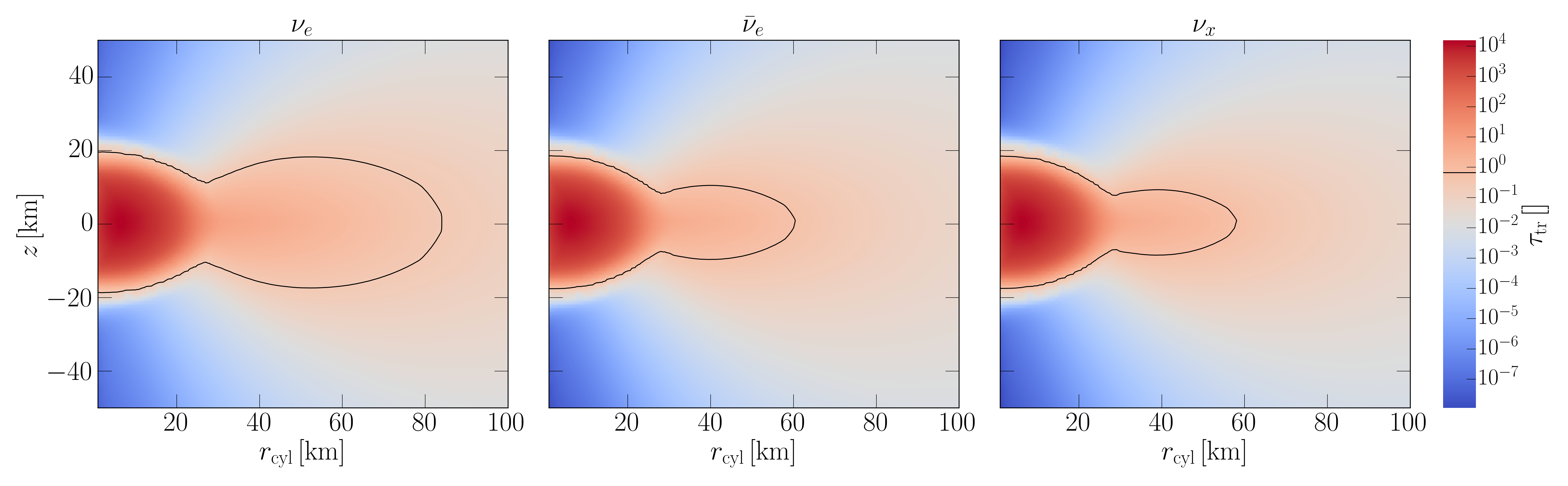
Figure 3: Transport optical depths $\tau$ (color coded) as functions of cylindrical coordinates $z$ and $r_{\mathrm{cyl}}$ at $t=100\,\mathrm{ms}$ after the merger. The contours (where $\tau\approx 2/3$) correspond to the neutrino transport surfaces associated with $\nu_{e}$ (left), $\bar{\nu}_{e}$ (middle) and $\nu_{x}$ (right).

In the following we construct an infinitely thin disk, i.e., we turn the neutrino surface into a flat disk, assume a constant temperature, and define the neutrino disk radius $R_{\nu}$ as the outermost radius of the neutrino surface,

$$R_{\nu}\equiv\max_{(r_{\mathrm{cyl}},z)\in S_{\nu}}\left\{\sqrt{r_{\mathrm{cyl}}^{2}+z^{2}}\right\}.$$ (7)

As can be seen from the results shown in Table 2, the differences in the neutrino surface radii for the two time snapshots of 60 ms and 100 ms, that we have used in our calculations, are only minor. The neutrino mean energies and luminosities are approximately stationary during the time of simulation Perego et al. (2014). The values, used in our calculations, are listed in Table 3.

Table 2: Outermost radii of the neutrino surfaces (at 60 ms and 100 ms) (see text).

t [ms]	$R_{\nu_{e}}$ [km]	$R_{\bar{\nu}_{e}}$ [km]	$R_{\nu_{x}}$ [km]
60	$90$	$64$	$61$
100	$84$	$60$	$58$

Table 3: Emission parameters with $\nu_{x}\in\{\nu_{\mu},\nu_{\tau},\bar{\nu}_{\mu},\bar{\nu}_{\tau}\}$.

Neutrino species	$\langle E_{\nu}\rangle$ [MeV]	$(L_{\nu}/10^{51})$ [erg/s]
$\nu_{e}$	$10.6$	$15$
$\bar{\nu}_{e}$	$15.3$	$30$
$\nu_{x}$	$17.3$	$8$

III Neutrino flavor transformation: Method

III.1 Equations of motion

To follow the flavor evolution of neutrinos emitted from the disk, we describe a mixed neutrino ensemble by Wigner distributions $\rho(\mathbf{p}^{\prime},\mathbf{x})$ with momentum $\mathbf{p}^{\prime}$ at location $\mathbf{x}$ Sigl and Raffelt (1993). In flavor space, these represent generalized occupation number matrices. In the neutrino free-streaming limit and assuming the system in a stationary state, the spatial evolution of $\rho(\mathbf{p}^{\prime},\mathbf{x})$ obeys the equation of motion at the lowest order Sigl and Raffelt (1993):

$$\mathbf{v}_{\mathbf{p}^{\prime}}\cdot\bm{\nabla}_{\mathbf{x}}\rho(\mathbf{p}^{\prime},\mathbf{x})=-i\left[\mathsf{H}(\mathbf{p}^{\prime},\mathbf{x}),\rho(\mathbf{p}^{\prime},\mathbf{x})\right],$$ (8)

where

$$\mathsf{H}=\mathsf{H}_{\mathrm{vac}}+\mathsf{H}_{\mathrm{matt}}+\mathsf{H}_{\nu\nu}$$ (9)

denotes the Hamiltonian including the vacuum, matter and neutrino potentials. Notice that we do not include external forces (such as gravity) acting on neutrinos $(\nabla_{\mathbf{p}}\rho=0)$ and follow neutrinos on straight-line paths. For antineutrinos we use $\bar{\rho}(\mathbf{p}^{\prime},\mathbf{x})$ with the same definition as in Sigl and Raffelt (1993) so that an analogous equation holds with the replacement $\mathsf{H}_{\mathrm{vac}}\mapsto-\mathsf{H}_{\mathrm{vac}}$. On the left hand side of Eq. (8) one recognizes the drift term of the Liouville-Vlasov operator, that is caused by the free streaming of neutrinos propagating with velocity $\mathbf{v}_{\mathbf{p}^{\prime}}$. In the following we use the ultra-relativistic approximation $|\mathbf{v}_{\mathbf{p}^{\prime}}|\approx c$.

Before giving the explicit form of terms in Eq. (9), we make a few remarks regarding Eq. (8). First, this equation of motion is valid at the mean-field level. However, the most general mean-field approximation includes extra contributions, in particular neutrino-antineutrino pairing correlations and mass corrections Volpe et al. (2013); Vlasenko et al. (2014b); Serreau and Volpe (2014); Cirigliano et al. (2015); Kartavtsev et al. (2015); Volpe (2015). The role of these terms still needs to be fully assessed. Second, we only study the limit where coherent forward scattering applies and sharply separate the dense region inside the neutrino surface, where neutrinos are trapped by collisions and the free streaming region. However, it was shown that in the context of core-collapse supernovae, the inclusion of a small backward scattered neutrino flux can affect the flavor evolution significantly Cherry et al. (2012). Including these effects in numerical simulations is challenging and beyond the scope of this work. Future efforts along these lines may be necessary.

Now, let us discuss the different terms contributing to the Hamiltonian in Eq. (9). The first one describes the vacuum term in the flavor basis, i.e.,

$$\mathsf{H}_{\mathrm{vac}}=\dfrac{1}{2E}\mathsf{U}\tilde{\mathsf{M}}^{2}\mathsf{U}^{\dagger},$$ (10)

where $E\approx|\mathbf{p}^{\prime}|$ corresponds to the energy of the neutrino and $\mathsf{U}$ denotes the Pontecorvo-Maki-Nakagawa-Sakata unitary mixing matrix Maki et al. (1962) which links weak flavor and vacuum mass eigenstates. The quantity $\tilde{\mathsf{M}}^{2}\equiv\mathrm{diag}[0,\Delta m_{21}^{2},\Delta m_{31}^{2}]$ essentially corresponds to the neutrino mass-squared matrix, where $\Delta m_{21}^{2}$ and $\Delta m_{31}^{2}$ denote the mass squared differences. The second term of the Hamiltonian Eq. (9) takes into account neutrino coherent forward scattering off electrons. Explicitly, we have

$$\mathsf{H}_{\mathrm{matt}}(\mathbf{x})=\sqrt{2}\mathrm{G}_{\mathrm{F}}n_{e}(\mathbf{x})\mathrm{diag}[1,0,0],$$ (11)

where $n_{e}=\rho_{\mathrm{matt}}Y_{e}/m_{\mathrm{u}}$ is the electron number density, determined by the matter density $\rho_{\mathrm{matt}}$ and electron fraction $Y_{e}$. Here, $m_{\mathrm{u}}$ denotes the unified atomic mass unit.

Similarly, we consider neutrino coherent forward scattering off neutrinos which introduces the non-linear nature of the problem:

$$\mathsf{H}_{\nu\nu}(\mathbf{p}^{\prime},\mathbf{x})=\sqrt{2}\mathrm{G}_{\mathrm{F}}\int\dfrac{\mathrm{d}^{3}p}{(2\pi)^{3}}\,(1-\mathbf{\hat{p}}^{\prime}\cdot\mathbf{\hat{p}})\left(\rho(\mathbf{p},\mathbf{x}){-}\bar{\rho}(\mathbf{p},\mathbf{x})\right),$$ (12)

where ${\mathbf{\hat{p}^{\prime}}=\mathbf{p}^{\prime}/|\mathbf{p}^{\prime}|}$ and ${\mathbf{\hat{p}}=\mathbf{p}/|\mathbf{p}|}$ denote unit vectors. In Eq. (12) $\rho(\mathbf{p},\mathbf{x})$ can be decomposed Qian and Fuller (1995); Fuller and Qian (2006) according to

$$\dfrac{\mathrm{d}^{3}p}{(2\pi)^{3}}\,\rho(\mathbf{p},\mathbf{x})=\sum_{\alpha=e,\mu,\tau}\mathrm{d}n_{\nu_{\underline{\alpha}}}(\mathbf{p},\mathbf{x})\,\rho_{\nu_{\underline{\alpha}}}(\mathbf{p},\mathbf{x})$$ (13)

for neutrinos in a differential volume element $\mathrm{d}^{3}p$ centered at momentum $\mathbf{p}$. A similar relation holds for antineutrinos. In Eq. (13) we introduced the initial (i.e., at the neutrino surface, denoted by an underline) differential neutrino number density $\mathrm{d}n_{\nu_{\underline{\alpha}}}$ and the single density $(3\times 3)$-matrices $\rho_{\nu_{\underline{\alpha}}}(\mathbf{p},\mathbf{x})$ for a neutrino with initial flavor $\alpha$ and momentum $\mathbf{p}$ at position $\mathbf{x}$. For normalization we choose the trace equal to one. The diagonal elements of the single density matrices correspond to the probabilities that a neutrino with initial flavor $\alpha$ can be found in a particular flavor $\beta$, i.e., $(\rho_{\nu_{\underline{\alpha}}})_{\beta\beta}=P(\nu_{\underline{\alpha}}\to\nu_{\beta})$, while the (complex-valued) off-diagonal elements describe quantum correlations between different neutrino flavors with the same momentum. An analogous relation holds for antineutrinos.

Using Eq. (13), Eq. (12) becomes:

$$\mathsf{H}_{\nu\nu}(\mathbf{p}^{\prime},\mathbf{x})=\sqrt{2}\mathrm{G}_{\mathrm{F}}\sum_{\alpha=e,\mu,\tau}\left(\int\mathrm{d}n_{\nu_{\underline{\alpha}}}\,(1-\mathbf{\hat{p}}^{\prime}\cdot\mathbf{\hat{p}})\rho_{\nu_{\underline{\alpha}}}(\mathbf{p},\mathbf{x})-\int\mathrm{d}n_{\bar{\nu}_{\underline{\alpha}}}\,(1-\mathbf{\hat{p}}^{\prime}\cdot\mathbf{\hat{p}})\bar{\rho}_{\bar{\nu}_{\underline{\alpha}}}(\mathbf{p},\mathbf{x})\right).$$ (14)

If we follow the flavor evolution of neutrinos along a specific trajectory, we can replace $\mathbf{v}_{\mathbf{p}}\cdot\mathbf{\nabla}_{\mathbf{x}}$ by a differential operator $\partial/\partial r$ along their direction of propagation so that the equations of motion (8) for the single density flavor matrices become:

$$\dfrac{\partial}{\partial r}\rho_{\nu_{\underline{\alpha}}}(\mathbf{p}^{\prime},\mathbf{Q}_{0},r) =-i[\mathsf{H}_{\mathrm{vac}}+\mathsf{H}_{\mathrm{matt}}+\mathsf{H}_{\nu\nu},\rho_{\nu_{\underline{\alpha}}}(\mathbf{p}^{\prime},\mathbf{Q}_{0},r)],$$ (15)

$$\dfrac{\partial}{\partial r}\bar{\rho}_{\bar{\nu}_{\underline{\alpha}}}(\mathbf{p}^{\prime},\mathbf{Q}_{0},r) =-i[-\mathsf{H}_{\mathrm{vac}}+\mathsf{H}_{\mathrm{matt}}+\mathsf{H}_{\nu\nu},\bar{\rho}_{\bar{\nu}_{\underline{\alpha}}}(\mathbf{p}^{\prime},\mathbf{Q}_{0},r)],$$ (16)

where $\mathbf{Q}_{0}$ is the emission point of the neutrinos and $r=r(\mathbf{x})$ is the distance they have traveled.

III.2 Neutrino self-interaction Hamiltonian in disk geometry

We employ the formalism introduced in Dasgupta et al. (2008); Malkus et al. (2012) and explicitly construct the self-interaction Hamiltonian for neutrinos emitted from a disk. The coordinate system is defined in such a way, that the following relations for the basis vectors hold: $\hat{\mathbf{e}}_{x}=\hat{\mathbf{e}}_{r_{\mathrm{cyl}}}$ and $\hat{\mathbf{e}}_{y}=\hat{\mathbf{e}}_{\phi}$. This allows us to identify the $x$-coordinate with the cylindrical radius $r_{\mathrm{cyl}}$ (Fig. 4).

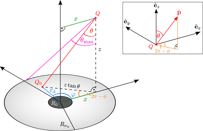
Figure 4: Accretion disk with a central object (black hole or neutron star) located at the origin. In case of a black hole, the radius $R_{0}$ denotes the last stable orbit and defines the inner radius of the disk while for a neutron star, we set $R_{0}=0$. The (outer) flavor dependent radii of the disk are $R_{\nu_{\alpha}}$ for neutrinos and $R_{\bar{\nu}_{\alpha}}$ for antineutrinos, respectively. The values used in our emission model are based on detailed simulations of a neutron star merger remnant Perego et al. (2014) and are given in Table 2. The polar angle $\theta$ and the azimuthal angle $\phi$ describe the direction of the neutrino momentum $\mathbf{p}$. Neutrinos are emitted from a point $Q_{0}$ located in the disk plane at a distance $r_{\mathrm{d}}$ from the origin with a relative angle $\varphi$ with respect to the positive $x$-axis and propagate to a point $Q$ located at a distance $x$ from the $z$-axis and a vertical distance $z$ from the equatorial plane.

At any point $\mathbf{Q}(x,0,z)$ on the $x$-$z$ plane, for a neutrino which is emitted from a point $\mathbf{Q}_{0}$ on the disk and passes through $\mathbf{Q}$, its momentum direction $\mathbf{\hat{p}}$ can be specified by a polar angle $\theta$ and an azimuthal angle $\phi$ in the spherical coordinate system (see Fig. 4):

$$\mathbf{\hat{p}}=(\sin{\theta}\cos{\phi},\sin{\theta}\sin{\phi},\cos{\theta}),$$ (17)

or by the polar coordinates $r_{\mathrm{d}}$ and $\varphi$ of the emission point $\mathbf{Q}_{0}(r_{\mathrm{d}},\varphi)$ on the disk:

$$\mathbf{\hat{p}}=\dfrac{\mathbf{Q}-\mathbf{Q}_{0}}{\Delta^{1/2}},$$ (18)

where

$$\Delta\equiv|\mathbf{Q}-\mathbf{Q}_{0}|^{2}=x^{2}+r_{\mathrm{d}}^{2}-2xr_{\mathrm{d}}\cos{\varphi}+z^{2}.$$ (19)

A comparison of Eq. (17) and Eq. (18) yields the following coordinate transformations:

$$\begin{split}\cos{\theta}&=\dfrac{z}{\Delta^{1/2}},\qquad\sin{\theta}=\dfrac{(\Delta-z^{2})^{1/2}}{\Delta^{1/2}},\\ \cos{\phi}&=\dfrac{x-r_{\mathrm{d}}\cos\varphi}{\Delta^{1/2}\sin\theta},\qquad\sin\phi=-\dfrac{r_{\mathrm{d}}\sin\varphi}{\Delta^{1/2}\sin\theta}\end{split}$$ (20)

with $\varphi\in[0,2\pi]$ and $r_{\mathrm{d}}\in[R_{0},R_{\nu}]$. We note that the determinant of the Jacobian $J\equiv\partial(\cos\theta,\phi)/\partial(r_{\mathrm{d}},\varphi)$ turns out to be

$$\mathrm{det}\,J =\dfrac{\partial(\cos\theta)}{\partial r_{\mathrm{d}}}\dfrac{\partial\phi}{\partial\varphi}-\dfrac{\partial(\cos\theta)}{\partial\varphi}\dfrac{\partial\phi}{\partial r_{\mathrm{d}}}$$ (21)

$$=-\dfrac{zr_{\mathrm{d}}}{\Delta^{3/2}},$$ (22)

such that $\mathrm{d}(\cos\theta)\mathrm{d}\phi=|\mathrm{det}\,J|\,\mathrm{d}r_{\mathrm{d}}\mathrm{d}\varphi$ holds.

Now, we consider another neutrino with momentum direction

$$\mathbf{\hat{p}^{\prime}}=(\sin\theta^{\prime}\cos\phi^{\prime},\sin\theta^{\prime}\sin\phi^{\prime},\cos\theta^{\prime}).$$ (23)

The cosine of the scattering angle, ${\cos\Theta_{\mathbf{p}\mathbf{p^{\prime}}}\equiv\mathbf{\hat{p}}\cdot\mathbf{\hat{p}}^{\prime}}$, between the two neutrinos is then given by:

$$\begin{split}\cos\Theta_{\mathbf{p}\mathbf{p^{\prime}}}&=\cos\theta\cos\theta^{\prime}\\ &\quad+\sin\theta\sin\theta^{\prime}\left(\cos\phi\cos\phi^{\prime}+\sin\phi\sin\phi^{\prime}\right).\end{split}$$ (24)

If we make use of the above transformations we find:

$$\begin{split}\cos\Theta_{\mathbf{p}\mathbf{p^{\prime}}}&=\dfrac{z\cos\theta^{\prime}}{\Delta^{1/2}}+\dfrac{x\sin\theta^{\prime}\cos\phi^{\prime}}{\Delta^{1/2}}\\ &-\dfrac{r_{\mathrm{d}}\sin\theta^{\prime}\cos\phi^{\prime}\cos\varphi}{\Delta^{1/2}}-\dfrac{r_{\mathrm{d}}\sin\theta^{\prime}\sin\phi^{\prime}\sin\varphi}{\Delta^{1/2}}.\end{split}$$ (25)

For neutrinos emitted isotropically from any point on the disk, the differential neutrino number density in Eq. (14) is given by:

$$\mathrm{d}n_{\nu_{\underline{\alpha}}}\equiv\mathrm{d}n_{\nu_{\underline{\alpha}}}(\mathbf{p})=j_{\nu_{\underline{\alpha}}}(E)\mathrm{d}E\mathrm{d}\Omega_{\nu_{\alpha}},$$ (26)

where $E=|\mathbf{p}|\equiv p$, $\mathrm{d}\Omega_{\nu_{\alpha}}\equiv\mathrm{d}\phi\mathrm{d}(\cos\theta)$ and $j_{\nu_{\underline{\alpha}}}$ denotes the neutrino number flux per unit energy per solid angle for which we assume a Fermi-Dirac shape (see Appendix B):

$$j_{\nu_{\underline{\alpha}}}(E)=\dfrac{F_{\nu_{\underline{\alpha}}}}{2\pi}f_{\nu_{\underline{\alpha}}}(E).$$ (27)

Here, $F_{\nu_{\underline{\alpha}}}=L_{\nu_{\underline{\alpha}}}/(\pi R_{\nu_{\alpha}}^{2}\langle E_{\nu_{\underline{\alpha}}}\rangle)$ corresponds to the neutrino number flux at the neutrino emitting surface and $f_{\nu_{\underline{\alpha}}}$ denotes the normalized Fermi-Dirac energy distribution function corresponding to the right hand site of Eq. (5) with $T=T_{\nu_{\underline{\alpha}}}$.

Inserting Eqs. (26) and (27) into Eq. (14), we rewrite the self-interaction Hamiltonian as:

$$\begin{split}\mathsf{H}_{\nu\nu}(\mathbf{p}^{\prime},\mathbf{Q}_{0},r)=\dfrac{\sqrt{2}\mathrm{G}_{\mathrm{F}}}{2\pi}\sum_{\alpha=e,\mu,\tau}\int_{0}^{\infty}\mathrm{d}E&\left(\int_{\Omega_{\nu_{\alpha}}}\mathrm{d}\Omega\,(1-\cos{\Theta_{\mathbf{p}\mathbf{p}^{\prime}}})\,F_{\nu_{\underline{\alpha}}}\rho_{\nu_{\underline{\alpha}}}(\Omega,\mathbf{Q}_{0},E,r)f_{\nu_{\underline{\alpha}}}(E)\right.\\ -&\left.\int_{\Omega_{\bar{\nu}_{\alpha}}}\mathrm{d}\Omega\,(1-\cos{\Theta_{\mathbf{p}\mathbf{p}^{\prime}}})\,F_{\bar{\nu}_{\underline{\alpha}}}\bar{\rho}_{\bar{\nu}_{\underline{\alpha}}}(\Omega,\mathbf{Q}_{0},E,r)f_{\bar{\nu}_{\underline{\alpha}}}(E)\right),\end{split}$$ (28)

where the angular integration is performed with the corresponding limits $\Omega_{\nu_{\alpha}(\bar{\nu}_{\alpha})}$ for neutrinos and antineutrinos, respectively.

III.3 Single-trajectory versus single- and multi-angle approximations

In order to follow the evolution, one should solve Eqs. (15) and (16) for all neutrinos with different $\mathbf{p}$ and $\mathbf{Q}_{0}$ simultaneously since $\mathsf{H}_{\nu\nu}$ couples them. This is computationally extremely demanding as we will discuss shortly. Instead of solving the full problem we employ a "single-trajectory" approximation which consists in making the assumption that in Eq. (28) the density matrix is given by

$$\rho_{\nu_{\underline{\alpha}}}(\Omega,\mathbf{Q}_{0},E,r)=\rho_{\nu_{\underline{\alpha}}}(\mathbf{p}^{\prime},\mathbf{Q}_{0},E,r),$$ (29)

that is, it does not dependent on the angular variables. In other words, we suppose that at every point of a given neutrino trajectory with momentum $\mathbf{p}^{\prime}$, all neutrino states contributing to $\mathsf{H}_{\nu\nu}(\mathbf{p}^{\prime},\mathbf{Q}_{0},r)$ have the same flavor evolution as the one with $\mathbf{p}^{\prime}$. The approximation given by Eq. (29) was already used in Malkus et al. (2012, 2014, 2016). We emphasize that this approach reduces to the “single-angle approximation” used in the supernova context for a spherically-symmetric system, such as the supernova bulb-model Duan et al. (2006). Note that the "multi-angle approximation" in the supernova bulb-model corresponds to retaining also the $\theta$ emission angle dependence in the self-interaction Hamiltonian.

At present, no simulations of neutrino flavor evolution in binary neutron star mergers exist where Eqs. (15) and (16) are solved without making the assumption Eq. (29). This is due to the fact that it may require computational capabilities beyond the current available resources. In fact, a multi-angle calculation in the supernova neutrino bulb-model, which only evolves the flavor content in the radial coordinate with one explicit emission angle variable, requires $\sim\mathcal{O}(10^{3})$ CPU hours Duan et al. (2006). Numerical convergence requires a large number of angle bins, typically of the order of $10^{3}$-$10^{4}$ Duan et al. (2006); Sarikas et al. (2012). In the disk case, performing a full calculation that preserves the initial symmetry of the system is much more complex than in the supernova bulb-model and requires to evolve the flavor content in both $x$ and $z$ coordinates with three explicit variables: $r_{\mathrm{d}}$, $\theta$, $\phi$ specifying the emission location and angles, respectively. As for the possible effect of going from the “single-trajectory” approximation to the full flavor calculation, one can speculate that this will introduce decoherence in the flavor evolution as in the supernova context multi-angle simulations have shown that occurs Dasgupta et al. (2009); Duan and Friedland (2011). Therefore the results presented here can be considered as an upper limit for the effects of flavor evolution on the capture rates since we expect that decoherence is likely to reduce them.

Now, under the single-trajectory approximation, Eqs. (15) and (16) can be solved for each density matrix $\rho_{\nu_{\underline{\alpha}}}=\rho_{\nu_{\underline{\alpha}}}(\theta_{0},\phi_{0},\mathbf{Q}_{0},E,r)$, and the angular integration yields a geometric factor

$$G_{\nu_{\alpha}}(\theta_{0},\phi_{0},\mathbf{Q}_{0},r)=\int_{\Omega_{\nu_{\alpha}}}\mathrm{d}\Omega\,(1-\cos{\Theta_{\mathbf{p}\mathbf{p}^{\prime}}}),$$ (30)

whose explicit form is described in Appendix C. Here, we fixed the emission angles $\theta_{0}$ and $\phi_{0}$ describing the direction of momentum $\mathbf{p}^{\prime}$. In Fig. 5 we show typical sizes for those factors. The ratio $G_{\nu_{e}}/G_{\bar{\nu}_{e}}$ increases as a function of distance.

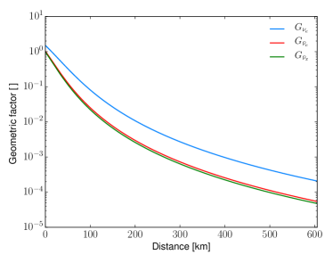
Figure 5: Geometric factors as function of the distance from the emission point $x_{0}=10\,\mathrm{km}$, $z_{0}=30\,\mathrm{km}$. The emission angles correspond to $\theta=20^{\circ}$ and $\phi=0^{\circ}$ while the disk radii are taken from Table 2.

In the following the explicit reference to the angular labels and the emission point will be omitted and the density matrices will be denoted just by $\rho_{\nu_{\underline{\alpha}}}(E,r)$ for notational convenience. Finally, the Hamiltonian Eq. (28) can be expressed in the compact form:

$$\begin{split}\mathsf{H}_{\nu\nu}(\theta_{0},\phi_{0},\mathbf{Q}_{0},r)=\sqrt{2}G_{\mathrm{F}}\sum_{\alpha=e,\mu,\tau}\int_{0}^{\infty}\mathrm{d}E&\,\left(\rho_{{\nu}_{\underline{\alpha}}}(E,r)j_{{\nu}_{\underline{\alpha}}}(E)G_{\nu_{\alpha}}(\theta_{0},\phi_{0},\mathbf{Q}_{0},r)\right.\\ &\left.-\bar{\rho}_{{\bar{\nu}}_{\underline{\alpha}}}(E,r)j_{{\bar{\nu}}_{\underline{\alpha}}}(E)G_{\bar{\nu}_{\alpha}}(\theta_{0},\phi_{0},\mathbf{Q}_{0},r)\right).\end{split}$$ (31)

IV Trajectory dependence of the unoscillated potentials

Flavor transformation through matter-neutrino resonances is an MSW-like phenomenon. Its occurrence is due to the almost cancellation of the matter and the neutrino self-interaction potentials, that have opposite signs. This condition is met for most neutrino trajectories in our model, since the self-interaction potential starts negative due to the dominating electron antineutrino fluxes (Table 3). However, for significant flavor conversions to occur, this nearly cancellation is not sufficient. Similar to the MSW case, it is the adiabaticity of the evolution that determines the flavor conversion efficiency Wu et al. (2016a); Väänänen and McLaughlin (2016); Malkus et al. (2014) and depends, beside the mixing parameters and the neutrino energy, on the matter profiles and their gradients.

We choose different neutrino emission points $(x_{0},z_{0})$ on the neutrino surfaces and compute their flavor evolution along trajectories that pass through two different reference points $(x_{\mathrm{ref}},z_{\mathrm{ref}})$ as given in Tables 4 and 5.

Table 4: Parameters that specify the neutrino trajectories: emission coordinates at the neutrino surface $(x_{0},z_{0})$ and emission angle $\theta_{0}$. The last column shows the distance between the emission point and the reference point $x_{\mathrm{ref}}=293\,\mathrm{km}$, $z_{\mathrm{ref}}=313\,\mathrm{km}$.

Trajectory	$x_{0}$ [km]	$z_{0}$ [km]	$\theta_{0}$ [∘]	Distance [km]
1a	$10$	$30$	$45.0$	$400$
1b	$-10$	$30$	$47.0$	$415$
1c	$-35$	$25$	$48.7$	$436$
1d	$50$	$30$	$40.7$	$373$

Table 5: Same as Table 4 for the reference point $x_{\mathrm{ref}}=74\,\mathrm{km}$, $z_{\mathrm{ref}}=206\,\mathrm{km}$.

Trajectory	$x_{0}$ [km]	$z_{0}$ [km]	$\theta_{0}$ [∘]	Distance [km]
2a	$10$	$30$	$20.0$	$187$
2b	$-10$	$30$	$25.5$	$195$
2c	$-35$	$25$	$31.1$	$211$
2d	$50$	$30$	$7.8$	$178$

To simplify the discussion, we implicitly assume that $\phi_{0}=0^{\circ}$, i.e., we do not explore the trajectory dependence on $\phi_{0}$. The two reference points are chosen to have a temperature $T=8\,\mathrm{GK}$ in different regions of the wind that give rise to different nucleosynthesis outcomes Martin et al. (2015). Point 1 (2) lies on $\approx 43^{\circ}$ $(20^{\circ})$ from the $z$-axis and is $\approx 429\,(219)\,\mathrm{km}$ away from the center of the MNS. Figure 6 shows the chosen neutrino emission points on the disk and the reference points 1 and 2 along with the density structure of the remnant.

For the mixing parameters we take values compatible with current best-fit values Olive et al. (2014): $\Delta m_{\mathrm{21}}^{2}=7.59\times 10^{-5}\,\mathrm{eV}^{2}$, $|\Delta m_{\mathrm{31}}^{2}|=2.43\times 10^{-3}\,\mathrm{eV}^{2}$, $\sin^{2}(2\theta_{12})=0.87$, $\theta_{13}=0.15$, $\theta_{23}=\pi/4$. We use $\delta_{\mathrm{CP}}=0$ for the CP-violating Dirac phase. Since the neutrino mass hierarchy is still unknown Qian and Vogel (2015), we consider both, the normal mass hierarchy (NH), i.e., $\Delta m_{31}^{2}>0$, and inverted mass hierarchy (IH), i.e., $\Delta m_{31}^{2}<0$.

Before presenting the numerical results we introduce the unoscillated potentials associated with the matter and the neutrino self-interaction terms of the Hamiltonian, as done in Malkus et al. (2012). The point where the sum of these two quantities cancel already gives an idea in which spatial region MNR are expected to occur.

As a measure for the matter strength, we use the refractive energy shift between $\nu_{e}$ and $\nu_{x}$ and define the neutrino-matter potential as follows:

$$\lambda(r)\equiv\sqrt{2}\mathrm{G}_{\mathrm{F}}n_{e}(r).$$ (32)

For the neutrino self-interaction, the individual contributions from $\nu_{x}$ exactly cancel at any point when flavor transformations have not occurred yet, since we assume the same initial fluxes and surface sizes. Hence, it is convenient to introduce the unoscillated neutrino self-interaction potential as follows:

$$\mu(r)\equiv\dfrac{\sqrt{2}\mathrm{G}_{\mathrm{F}}}{2\pi^{2}}\left\{\dfrac{L_{\nu_{\underline{e}}}}{\langle E_{\nu_{\underline{e}}}\rangle R_{\nu_{e}}^{2}}G_{\nu_{e}}(\theta_{0},\phi_{0},r)-\dfrac{L_{\bar{\nu}_{\underline{e}}}}{\langle E_{\bar{\nu}_{\underline{e}}}\rangle R_{\bar{\nu}_{e}}^{2}}G_{\bar{\nu}_{e}}(\theta_{0},\phi_{0},r)\right\}.$$ (33)

Note that the scales set by the vacuum potentials $\omega\equiv\Delta m^{2}/(2E)$ ($|\omega_{31}|\approx\,0.4\,\mathrm{km}^{-1}$ and $\omega_{21}\approx\,0.01\,\mathrm{km}^{-1}$ for a $15\,\mathrm{MeV}$ neutrino) are typically well below $\lambda(r)$ and |$\mu(r)$|.

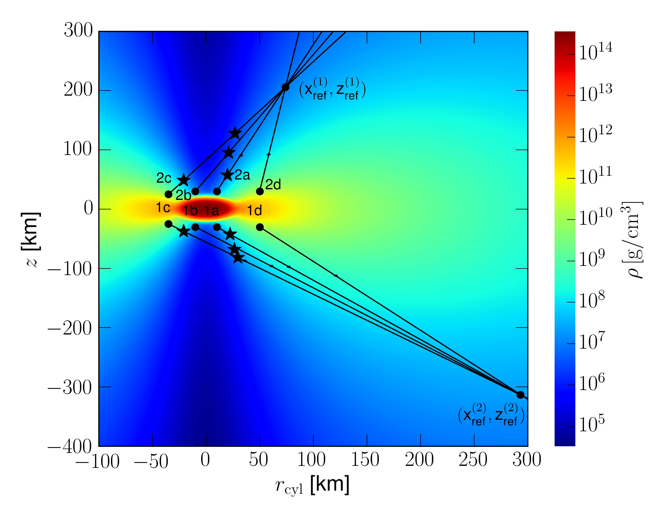
Figure 6: Density profile at $100\,\mathrm{ms}$ after the merger as a function of cylindrical coordinates $z$ and $r_{\mathrm{cyl}}$. The neutrino trajectories, shown by the black lines, are specified in Tables 4 and 5. We mirrored the trajectories of Table 4 for clarity. The two reference points $(x_{\mathrm{ref}}^{(i)},z_{\mathrm{ref}}^{(i)})$, $i=1,2$, are located at a temperature $T\approx 8\,\mathrm{GK}$ and chosen as representative locations interesting for nucleosynthesis. The points where the matter and unoscillated neutrino self-interaction potentials cancel are marked with $\bigstar$.

Let us discuss the trajectories listed in Tables 4 and 5 taken as representatives over the large set we explored. In the top panels of Figs. 7 and 8 we present the matter and unoscillated neutrino self-interaction potentials Eqs. (32) and (33) for these trajectories shown in Fig. 6. In addition we show the vacuum potentials $\omega_{21}$ and $|\omega_{31}|$ for $5\,\mathrm{MeV}$ (anti)neutrinos. To guide the eye we highlight the region around the location of the reference point with a color band. The initial points of 1a (2a) and 1b (2b) are located in the low density polar region, where the matter potential $\lambda$ is around $3\times 10^{3}\,\mathrm{km}^{-1}$ ($\rho_{\mathrm{matt}}\sim 2\times 10^{7}\,\mathrm{g}\,\mathrm{cm}^{-3}$, $Y_{e}\sim 0.39$); while trajectory 1c (2c) starts in a low density regime of the wind, where the matter potential is much stronger $9\times 10^{5}\,\mathrm{km}^{-1}$ ($\rho_{\mathrm{matt}}\sim 7\times 10^{9}\,\mathrm{g}\,\mathrm{cm}^{-3}$, $Y_{e}\sim 0.31$). The starting point of trajectory 1d (2d) is located deeper inside the wind where $\lambda\sim 1\times 10^{6}\,\mathrm{km}^{-1}$ ($\rho_{\mathrm{matt}}\sim 2\times 10^{10}\,\mathrm{g}\,\mathrm{cm}^{-3}$, $Y_{e}\sim 0.18$).

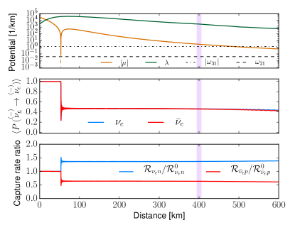
(a) 1a (NH): $x_{0}=10\,\mathrm{km}$, $z_{0}=30\,\mathrm{km}$, $\theta_{0}=45.0^{\circ}$

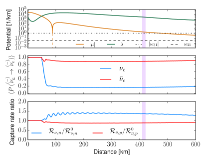
(b) 1b (NH): $x_{0}=-10\,\mathrm{km}$, $z_{0}=30\,\mathrm{km}$, $\theta_{0}=47.0^{\circ}$

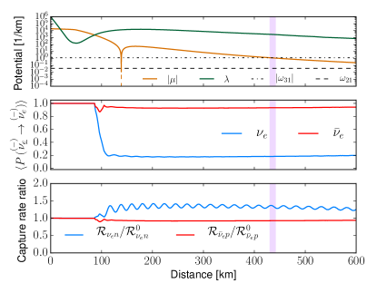
(c) 1c (NH): $x_{0}=-35\,\mathrm{km}$, $z_{0}=25\,\mathrm{km}$, $\theta_{0}=48.7^{\circ}$

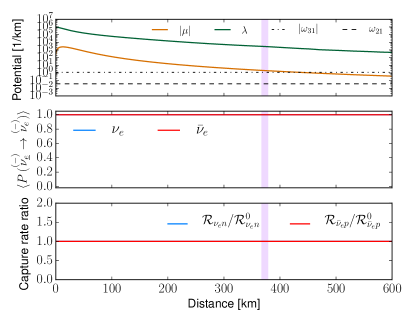
(d) 1d (NH): $x_{0}=50\,\mathrm{km}$, $z_{0}=30\,\mathrm{km}$, $\theta_{0}=40.7^{\circ}$

Figure 7: Results for selected trajectories specified in Table 4 as functions of the distance for the normal mass hierarchy. The location of the reference point is highlighted by a vertical color band. Top panels: matter potentials ($\lambda$) and absolute values of the unoscillated neutrino potentials ($|\mu|)$ along with the vacuum potentials $\omega_{21}$ and $|\omega_{31}|$ for $5\,\mathrm{MeV}$ (anti)neutrinos. The middle panels show the spectral averaged survival probabilities for the electron flavor. The blue curves correspond to $\nu_{e}$ and the red curves to $\bar{\nu}_{e}$, respectively. In the bottom panels, the ratios of capture rates per solid angle for electron neutrinos (blue) and antineutrinos (red) are presented.

Neutrinos on their way on trajectories 1a initially experience an increasing matter potential. When the wind becomes more dilute, the potential decreases until they reach the reference point. In case of trajectories 1b and 2b, neutrinos will first pass the funnel above the MNS pole where the density is very low compared to the emission region. When it enters the wind region the density increases. Afterwards neutrinos proceed similarly like in 1a, i.e., they go through the dilute part of the wind (matter potential is decreasing) and arrive at the reference point. For trajectories 1c and 2c, neutrinos will first need to cover some distance through the dense part of the wind before entering the funnel. Afterwards, they propagate in an analogous way like in cases 1b and 2b. The transition between wind and funnel leads to a rapid drop in the density which is clearly visible in Figs. 7 and 8 for trajectories 1b, 1c, 2b and 2c. A different behavior will be experienced by neutrinos following trajectories 1d, 2a, and 2d. They encounter a monotonically decreasing matter potential until they reach the reference point.

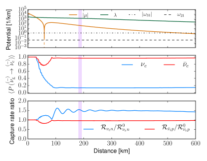
(a) 2a (NH): $x_{0}=10\,\mathrm{km}$, $z_{0}=30\,\mathrm{km}$, $\theta_{0}=20.0^{\circ}$

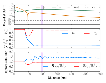
(b) 2b (NH): $x_{0}=-10\,\mathrm{km}$, $z_{0}=30\,\mathrm{km}$, $\theta_{0}=25.5^{\circ}$

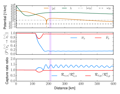
(c) 2c (NH): $x_{0}=-35\,\mathrm{km}$, $z_{0}=25\,\mathrm{km}$, $\theta_{0}=31.1^{\circ}$

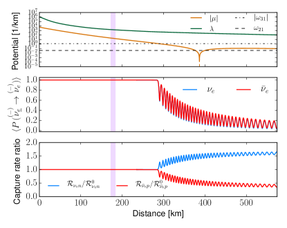
(d) 2d (NH): $x_{0}=50\,\mathrm{km}$, $z_{0}=30\,\mathrm{km}$, $\theta_{0}=7.8^{\circ}$

Figure 8: Same as Fig. 7 for the trajectories specified in Table 5.

In the self-interaction potential, the relative contribution of $\nu_{e}$ and $\bar{\nu}_{e}$ changes as a function of distance, due to the interplay of $j_{\nu_{\underline{\alpha}}}$ and $G_{\nu_{\underline{\alpha}}}$. In particular this means that initially, the neutrino self-interaction potential is negative, because it is dominated by the larger electron antineutrino fluxes. Later, the fact that the neutrino surface for electron neutrinos is larger than that of electron antineutrinos, may lead to a change of sign in the self-interaction potential (as we will see in Sec. V.1). The absolute values of the unoscillated neutrino potentials $|\mu(r)|$ vary between $\sim 10^{4}\,\mathrm{km}^{-1}$ initially to $\sim 10^{-1}\,\mathrm{km}^{-1}$ at $600\,\mathrm{km}$. The relative magnitude of the matter and neutrino potentials and the possible presence of crossings will determine the flavor evolution as we will see in Sec. V.1. We find that the crossings happen at the edge of the funnel (see Fig. 6). This means that for neutrinos emitted around the central region and from the opposite side of the disk, their trajectories cross the funnel so that MNR may occur.

V Numerical Results

Our goal is to show the trajectory dependence of flavor evolution for neutrinos from the disk by presenting spectral-averaged flavor conversion probabilities (Sec. V.1). As we will discuss we find a variety of flavor conversion behaviors. Furthermore, we explore the potential impact on nucleosynthesis in the neutrino-driven wind by showing ratios of oscillated and unoscillated capture rates per solid angle (Sec. V.2). We present results based on hydrodynamical profiles obtained at 100 ms. We discuss possible variations with a different time snapshot (60 ms) in Sec. V.3. Finally, we show the sensitivity of the flavor evolution when employing different assumptions for the initial luminosities, or considering uncertainties on the neutrino fluxes from simulations available in the literature.

In our calculations of the flavor evolution we assume that all (anti-)neutrinos are prepared in flavor eigenstates. The flavor evolution of neutrinos with different energies is then followed by numerically solving Eqs. (15) and (16) with the Hamiltonian components given by Eqs. (10), (11), and (31) for a given trajectory with emission angle $\theta_{0}$. We employed different discretizaton schemes to check for convergence of the results.

V.1 Flavor conversion results and general behavior

After obtaining the flavor evolution of neutrinos along each trajectory, $\rho_{\nu_{\underline{\alpha}}}(E,r)$ and $\rho_{\bar{\nu}_{\underline{\alpha}}}(E,r)$, we compute spectral averages of the neutrino survival probability, i.e.,

$$\langle P(\nu_{\underline{e}}\to\nu_{e})\rangle(r)=\int_{0}^{\infty}\mathrm{d}E\,f_{\nu_{\underline{e}}}(E)P(\nu_{\underline{e}}\to\nu_{e})(E,r).$$ (34)

Notice that ${P(\nu_{\underline{\alpha}}\to\nu_{\beta})=(\rho_{\nu_{\underline{\alpha}}})_{\beta\beta}}$ as defined in Sec. III.1.

As examples, we show the averaged survival probabilities of electron neutrinos and antineutrinos for the trajectories 1a to 1d in the middle panels of Fig. 7 and 2a to 2d in Fig. 8. These results are obtained in NH.

As can be seen from Figs. 7 and 8 (top panels), the structure of some profiles allows the unoscillated potentials to cancel at more than one spatial location such as trajectories 1c and 2c. We indicate these locations in Fig. 6 for the trajectories defined in Tables 4 and 5. If the resonance condition is fulfilled, flavor conversion only occurs if the strength of the neutrino self-interaction is larger than the matter contribution ($\lambda<|\mu|$) prior to it. If the matter term dominates the self-interaction term ($\lambda>|\mu|$), before a cancellation point, the resonances are extremely non-adiabatic and nearly no flavor transformation can happen Wu et al. (2016a); Malkus et al. (2014). The characteristic feature of the standard MNR is that electron neutrinos can undergo significant flavor change, while electron antineutrinos only experience little flavor conversion. This is due to the fact that the latter go through their resonances extremely non-adiabatically at either the beginning or the end of the MNR, depending on the hierarchy, in a way similar to the results shown in Wu et al. (2016a) with 2-flavor toy models. In NH, we find that survival probabilities for neutrinos propagating along trajectories 1b, 1c, 2a, 2b, and 2c exhibit the standard MNR features discussed above. We note that in all MNR cases, high energy $\nu_{e}$ are only partially converted at the end of the MNR region, resulting in a $\sim 20\%$ averaged survival probabilities.

For trajectory 1a, despite the MNR condition is fulfilled, the flavor transformation is extremely non-adiabatic and nearly no flavor conversion happens immediately after the MNR location. However, at $\sim 50$ km, we see that both $\nu_{e}$ and $\bar{\nu}_{e}$ undergo simultaneous flavor conversions when $\lambda(r)\gg|\mu(r)|$. This is due to the fact that the $\nu\nu$ coupling introduces a synchronization frequency  Pastor and Raffelt (2002):

$$\omega_{\mathrm{sync}}^{ij}(r)\approx\dfrac{\sqrt{2}G_{\mathrm{F}}\int\mathrm{d}E\,\omega_{ij}[j_{\nu_{\underline{e}}}(E)G_{\nu_{e}}(r)+j_{\bar{\nu}_{\underline{e}}}(E)G_{\bar{\nu}_{e}}(r)]}{\mu(r)}.$$ (35)

As $|\mu(r)|\rightarrow 0$ when it changes sign, $|\omega^{ij}_{\rm sync}(r)|\propto|1/\mu(r)|$ can be very large. Thus, a synchronized MSW effect (see, e.g., Wong (2002); Abazajian et al. (2002)) happens when $\omega^{ij}_{\rm sync}\cos{\theta_{ij}}\sim\lambda$ so that all neutrinos and antineutrinos with different momenta are bound together and simultaneously go through the MSW-like flavor conversion. We note here that the flavor transformation is actually due to the resonance of $\omega^{21}_{\rm sync}$ with $\lambda(r)$ as the larger mixing angle $\theta_{12}$ provides enough adiabaticity.

For 1d and 2d, the MNR condition is not met and there is no flavor conversion in 1d. However, 2d shows synchronized type oscillations starting at $\sim 285$ km, resulting both $\nu_{e}$ and $\bar{\nu}_{e}$ flavor conversions.

For IH, the qualitative behaviors are the same as in NH when MNR occurs (1b, 1c, 2a, 2b, 2c). The only difference is the slightly more adiabatic flavor transformation near the end of the MNR region (see Fig. 9 for the example of 2a). Regarding the other trajectories, we find for 1a (as in NH) the same synchronized MSW conversion while 1d and 2d, now show the “bipolar” type of flavor transformation (see e.g., Duan et al. (2010)) so that both $\nu_{e}$ and $\bar{\nu}_{e}$ are transformed, but their averaged survival probabilities are different (see Fig. 9 for the example of 2d).

We provide a summary of the results in Table 6, where we report the type of flavor conversion mechanism.

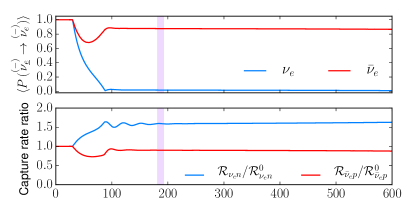
(a) 2a

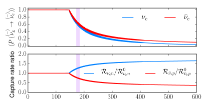
(b) 2d

Figure 9: Flavor evolution results obtained in IH along trajectories 2a (top) and 2d (bottom). The top panels show the spectral averaged survival probabilities for the electron flavor. The blue curves correspond to $\nu_{e}$ and the red ones to $\bar{\nu}_{e}$, respectively. In the bottom panels the ratios of capture rates per solid angle for electron neutrinos (blue) and antineutrinos (red) are presented.

Table 6: For the given trajectories, we list the flavor conversion mechanism (MNR, synchronized MSW (sync.), bipolar, and no conversion (-)) and capture rate ratios for $\nu_{e}$ and $\bar{\nu}_{e}$ (distance-averaged around the location of the reference point ($T=8\,\mathrm{GK}$)) and both mass hierarchies.

Trajectory	Flavor conversion		Capture rate ratio
	NH	IH	NH		IH
			$\nu_{e}$	$\bar{\nu}_{e}$	$\nu_{e}$	$\bar{\nu}_{e}$
1a	sync.	sync.	+36%	-36%	+67%	-67%
1b	MNR	MNR	+37%	-11%	+46%	-12%
1c	MNR	MNR	+33%	-7%	+43%	-7%
1d	-	bipolar	-	-	+46%	-49%
2a	MNR	MNR	+52%	-4%	+59%	-10%
2b	MNR	MNR	+39%	-4%	+56%	-8%
2c	MNR	MNR	+37%	-4%	+53%	-6%
2d	sync.	bipolar	-	-%	+26%	-25%

V.2 Differential capture rates

We calculate the rate per solid angle for electron neutrino captures on free neutrons with both the oscillated and unoscillated neutrino spectra. The oscillated rate is given by:

$$\begin{split}\mathcal{R}_{\nu_{e}n}(r)&=\dfrac{1}{2\pi}\sum_{\alpha=e,\mu,\tau}F_{\nu_{\underline{\alpha}}}\int_{0}^{\infty}\mathrm{d}E\,f_{\nu_{\underline{\alpha}}}(E)\\ &\qquad\times\sigma_{\nu_{e}n,\mathrm{abs}}(E)P(\nu_{\underline{\alpha}}\to\nu_{e})(E,r).\end{split}$$ (36)

For the unoscillated capture rate we use:

$$\mathcal{R}_{\nu_{e}n}^{0}=\dfrac{F_{\nu_{\underline{e}}}}{2\pi}\int_{0}^{\infty}\mathrm{d}E\,f_{\nu_{\underline{e}}}(E)\sigma_{\nu_{e}n,\mathrm{abs}}(E).$$ (37)

Similar expressions ($\mathcal{R}_{\bar{\nu}_{e}p}$, $\mathcal{R}_{\bar{\nu}_{e}p}^{0}$) hold for electron antineutrino capture on free protons with $\sigma_{\bar{\nu}_{e}p,\mathrm{abs}}$, where the lower bound of the integrals has to be replaced by the threshold $m_{e}+\Delta_{np}$, i.e., the sum of the electron mass $m_{e}\approx 0.5\,\mathrm{MeV}$ and the neutron-proton mass difference $\Delta_{np}$. We compute the ratio between oscillated $\mathcal{R}$ and unoscillated $\mathcal{R}^{0}$ capture rates.

From Eq. (36), one can see that when calculating $\mathcal{R}$, the electron neutrino appearance probabilities will be weighted by the $\nu_{\mu}$/$\nu_{\tau}$ fluxes (Eq. (79)) and the cross section (Eq. (38)). We note that the fluxes $j_{\nu_{\underline{\alpha}}}$ are peaked around $2.2\,T_{\nu_{\underline{\alpha}}}$ while the rates $(j_{\nu_{\underline{\alpha}}}\sigma)$ around $4.1\,T_{\nu_{\underline{\alpha}}}$ (Fig. 10). Therefore, for $\mathcal{R}_{\nu_{e}n}$, the contribution of the initial non-electron flavors will enhance it when efficient $\nu_{e}\leftrightarrow\nu_{x}$ flavor conversion took place, as the high energy tail of the initial $\nu_{x}$ dominates the capture rates indicated in Fig. 10. For $\mathcal{R}_{\bar{\nu}_{e}p}$, from Fig. 10 wee see that since $(j_{\bar{\nu}_{\underline{e}}}\sigma_{\bar{\nu}_{e}p,{\rm abs}})>(j_{\nu_{\underline{\mu,\tau}}}\sigma_{\bar{\nu}_{e}p,{\mathrm{abs}}})$ for the whole energy spectrum, any flavor conversion of $\bar{\nu}_{e}\leftrightarrow\bar{\nu}_{x}$ will suppress it.

Based on the above discussions, we see from the bottom panels of Figs. 7, 8, and 9 that for $\nu_{e}$ which undergo efficient flavor conversions due to MNR (1b, 1c, 2a, 2b, 2c), the $\nu_{e}$ capture rates are largely enhanced by up to $\sim 59\%$ after the end of the MNR region while the $\bar{\nu}_{e}$ capture rates are slightly decreased by up to $\sim 12\%$ in those cases. For the trajectories showing the synchronized MSW flavor transformation (1a), the $\nu_{e}$ ($\bar{\nu}_{e}$) capture rates are increased (decreased) by up to $\sim 67\%$ $(67\%)$ as both are simultaneously transformed. As for the cases with bipolar type of flavor conversion (1d and 2d in IH), the capture rates for $\nu_{e}$ ($\bar{\nu}_{e}$) are gradually changed up to $\sim 65\%$ ($-62\%$) at $600$ km. In most cases where flavor conversion takes place, the capture rates are affected in regions with temperature $T\gtrsim 8\,\mathrm{GK}$ before all nucleons recombine into $\alpha$-particles. We provide a summary of the capture rate ratio, $\mathcal{R}/\mathcal{R}^{0}$, in Table 6 at the reference locations ($T=8$ GK) for all trajectories.

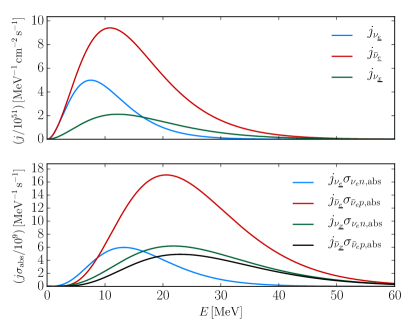
Figure 10: Neutrino number fluxes [see (27)] (upper panel) and number fluxes times cross sections (lower panel). All quantities are per unit energy per solid angle.

V.3 Comparison between different post-merger times

Although the neutrino luminosities and average energies remain nearly stationary over the disk evolution time, the wind density profiles change substantially. In Fig. 11, we compare the matter potentials for trajectories 2a (upper) and 2c (lower panel) at different times ($60$ and $100\,\mathrm{ms}$). For both cases, the matter potentials are larger at $100\,\mathrm{ms}$ compared to the one at $60\,\mathrm{ms}$ and show a similar overall behavior as a function of distance. This is because the expanding wind drives the surrounding area less neutron-rich at later times, as can be inferred from Figs. 2 and 12. Consequently, the MNR locations at $100\,\mathrm{ms}$ are shifted to smaller distances. However, such differences do not result in qualitative changes in the overall flavor evolution behavior.

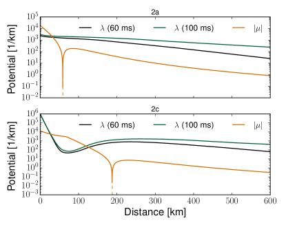
Figure 11: Comparison of the unoscillated potentials between the time snapshots for trajectories 2a (upper) and 2c (lower panel).

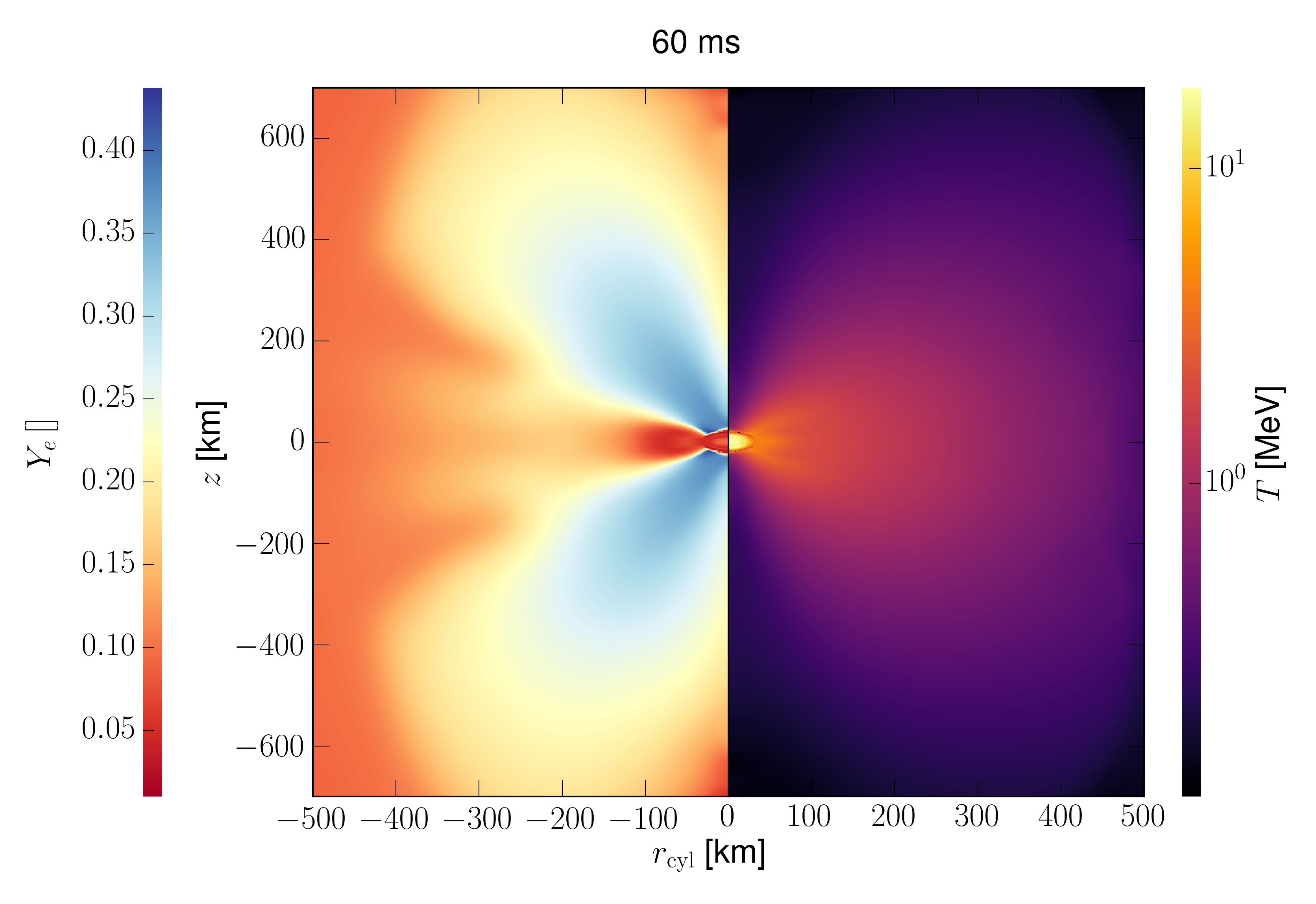
Figure 12: Electron fraction (left panel) and matter temperature (right panel) as functions of cylindrical coordinates $z$ and $r_{\mathrm{cyl}}$ at $t=60\,\mathrm{ms}$ after the merger.

V.4 Impact of input neutrino emission characteristics

For the results presented so far, the calculations are performed based on the neutrino luminosities and mean energies given in Table 3. These values are obtained at distances far away from the disk, which are called “net luminosities” in Perego et al. (2014) (see Fig. 8 of Perego et al. (2014)). However, neutrinos do not completely travel unhindered from the neutrino surfaces in a realistic environment. Their luminosities can be higher in regions close to the neutrino surfaces and reduce to the net luminosities due to charged-current neutrino absorptions above the surfaces. Since the environment is neutron-rich, the decrease of $L_{\nu_{e}}$ is larger than that of $L_{\bar{\nu}_{e}}$ and $L_{\nu_{x}}$. Consequently, a less negative $\mu(r)$ compared to the values obtained with net luminosities in regions close to the neutrino surfaces may be obtained. If for a trajectory, $|\mu(r)|>\lambda(r)$ initially close to the neutrino surfaces, one expects MNR to occur closer to the emission point.

We explore this effect by performing additional calculations for all trajectories using the “cooling” neutrino luminosities from (Perego et al., 2014), calculated by neglecting charged-current neutrino absorptions above the neutrino surfaces: $L_{\nu_{e},{\rm cool}}=25\times 10^{51}$ erg s ^-1, $L_{\bar{\nu}_{e},{\rm cool}}=33\times 10^{51}$ erg s ^-1, and $L_{\nu_{x},{\rm cool}}=L_{\nu_{x}}=8\times 10^{51}$ erg s ^-1. Compared to the net luminosities (see Table 3), $L_{\nu_{e},{\rm cool}}=1.67L_{\nu_{e}}$ and $L_{\bar{\nu}_{e},{\rm cool}}=1.1L_{\bar{\nu}_{e}}$. Figure 13 shows the results with cooling luminosities for trajectories 1c and 2a. In both cases, the MNR locations with a larger $L_{\nu_{e},{\rm cool}}$ are indeed closer to their emission points when compared to Fig. 7 and 8. In 1c, MNR now occurs at $\sim 66$ km immediately prior to the point where $\mu$ changes sign. This results in a complete flavor transformation for both $\nu_{e}$ and $\bar{\nu}_{e}$, or symmetric MNR Malkus et al. (2012, 2016). After the symmetric MNR, another standard MNR occurs at a distance of $\sim 82$ km so that antineutrinos go through nearly complete flavor conversion as discussed in Malkus et al. (2016). For the capture rate ratio of $\nu_{e}$, it only change slightly due to a much higher $L_{\nu_{e},{\rm cool}}$. For $\bar{\nu}_{e}$, the capture rate ratio is largely suppressed in the region between the symmetric MNR and the second standard MNR. For case 2a, the position where MNR occurs is also largely shifted to a smaller distance at $\sim 10$ km. However, we find a strongly non-adiabatic behavior resulting in no flavor transformation.

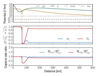
(a) 1c (NH)

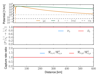
(b) 2a (NH)

Figure 13: Same as Fig. 7 for trajectories 1c (left) and 2a (right) with cooling luminosities (see text).

The model we have considered is based on one particular simulation of the remnant from the merger of BNS with equal mass. The large variety of possible initial conditions of the merger (NS masses and spins, mass ratios) is expected to translate into a wide range of both the neutrino luminosities and the mean energies for different systems. Also, the neutrino emissions can be significantly influenced by the thermodynamical properties of the dense nuclear matter, which is subject to the large uncertainties in the nuclear equation of state (EOS, see e.g. Sekiguchi et al. (2015); Foucart et al. (2016) for the potential impact of the nuclear EOS on the neutrino luminosities). Lastly, the different numerical techniques and levels of approximations that are used to model hydrodynamics, gravity and weak interactions can all lead to quantitatively different predictions of the relevant neutrino quantities. To quantify these uncertainties in our input parameters, we have collected published values of neutrino luminosities and mean energies (when available) from several different simulations of BNS merger and of the merger aftermath in presence of a long lived MNS. We show these values in Table 7 in Appendix D. We see that the luminosities may differ by one order of magnitude while the differences in mean energies are within a factor of two. We show in Figs. 14 and 15 the ratio of luminosities, $L_{\bar{\nu}_{e}}/L_{\nu_{e}}$ and $L_{\nu_{e}}/L_{\nu_{x}}$, and the ratio of mean energies, $\langle E_{\bar{\nu}_{e}}\rangle/\langle E_{\nu_{e}}\rangle$ and $\langle E_{\nu_{e}}\rangle/\langle E_{\nu_{x}}\rangle$. We emphasize that our goal is not to compare the results of the different simulations, but to show the variety of possible ranges for these ratios.

Note that the neutrino self-interaction potential depends on the difference between the fluxes of neutrinos and antineutrinos, which are proportional to the neutrino number luminosities $\sim L_{\nu_{\alpha}}/\langle E_{\nu_{\alpha}}\rangle$. We further show the corresponding ratios, $(L_{\bar{\nu}_{e}}/\langle E_{\bar{\nu}_{e}}\rangle)/(L_{\nu_{e}}/\langle E_{\nu_{e}}\rangle)$ and $(L_{\nu_{e}}/\langle E_{\nu_{e}}\rangle)/(L_{\nu_{x}}/\langle E_{\nu_{x}}\rangle)$ in Fig. 16.

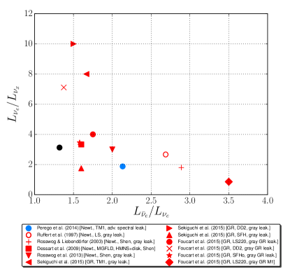
Figure 14: Ratio of luminosities: $L_{\nu_{e}}/L_{\nu_{x}}$ vs. $L_{\bar{\nu}_{e}}/L_{\nu_{e}}$. The corresponding values are given in Table 7. The black point refers to the cooling luminosities of Perego et al. (2014) (see text).

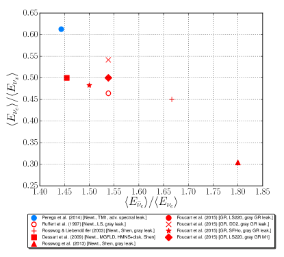
Figure 15: Ratio of mean energies: $\langle E_{\nu_{e}}\rangle/\langle E_{\nu_{x}}\rangle$ vs. $\langle E_{\bar{\nu}_{e}}\rangle/\langle E_{\nu_{e}}\rangle$. The corresponding values are given in Table 7.

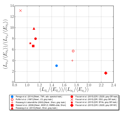
Figure 16: Ratio of emission rates: $(L_{\nu_{e}}/E_{\nu_{e}})/(L_{\nu_{x}}/E_{\nu_{x}})$ vs. $(L_{\bar{\nu}_{e}}/E_{\bar{\nu}_{e}})/(L_{\nu_{e}}/E_{\nu_{e}})$. The corresponding values are given in Table 7.

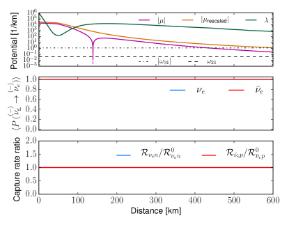
(a) 1c (NH): $x_{0}=-35\,\mathrm{km}$, $z_{0}=25\,\mathrm{km}$, $\theta_{0}=48.7^{\circ}$

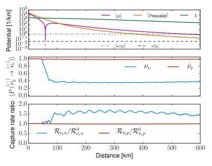
(b) 2a (NH): $x_{0}=10\,\mathrm{km}$, $z_{0}=30\,\mathrm{km}$, $\theta_{0}=20.0^{\circ}$

Figure 17: Same as Fig. 7 for trajectories 1c and 2a with rescaled fluxes (see text).

To explore the impact of different flux ratios on the neutrino flavor evolution, we have varied the neutrino luminosities of Table 3 by: $L_{\nu_{e}}\mapsto 0.65\,L_{\nu_{e}}$ and $L_{\nu_{x}}\mapsto 1.16\,L_{\nu_{x}}$. This change gives a similar $(L_{\bar{\nu}_{e}}/\langle E_{\bar{\nu}_{e}}\rangle)/(L_{\nu_{e}}/\langle E_{\nu_{e}}\rangle)$ to the value obtained in Foucart et al. (2016) [GR, gray GR M1, LS220 EOS] Foucart et al. (2016). The results with such luminosities for trajectories 1c and 2a in NH are shown in Fig. 17. Contrary to the previously discussed exploration with cooling luminosities, the differences between the fluxes of electron neutrinos and electron antineutrino becomes larger. This affects the self-interaction potential in such a way that no change of sign in $\mu(r)$ occurs anymore.

For trajectory 1c, the flavor evolution becomes strongly non-adiabatic when compared to the result shown in Fig. 7c. For trajectory 2a, the flavor evolution becomes less adiabatic.

VI Discussion and Conclusions

In the present work, we investigated the trajectory dependence of the neutrino flavor evolution in a BNS merger remnant. We found that depending on which location and which polar angle neutrinos are emitted, the outcome can be different. In particular, we observed that flavor conversion through MNR can occur for most neutrinos traveling through the low density funnel. For cases without flavor conversion across MNR due to the non-adiabaticity, a synchronized MSW transformation can take place afterwards. For neutrinos that do not encounter MNR, bipolar type of flavor oscillations may occur for the IH. We note that future investigations should also explore the dependence on the azimuthal emission angle that was omitted in this work.

We found that flavor evolution can significantly affect the neutrino capture rates on protons and neutrons at the regions with $T\gtrsim 8\,\mathrm{GK}$. This may change the $r$-process abundances in the neutrino wind. In our work we presented capture rates which do not take into account the solid angle contributions. This treatment is consistent with our single-trajectory approximation and we found that the oscillated $\nu_{e}$ ($\bar{\nu}_{e}$) capture rates can increase (decrease) up to almost 67% (67%).

If we apply flavor conversion probabilities derived with the single-trajectory approximation to all neutrinos emitted from the disk and integrate over the solid angle (see, e.g., Fig. 19), we find the $\nu_{e}$ capture rates instead always decrease. This behavior is due to the fact that the solid angle for $\nu_{e}$ is larger so that the relative contribution from $\nu_{x}$ reduces. We speculate that the use of the "single-trajectory" assumption is maximizing the impact of flavor conversion we find on the capture rates.

The initial luminosities are a key input for the flavor evolution as we observed. In fact, a change in the luminosities can produce different flavor conversion results. In particular, we have shown this fact in two ways: either by taking the cooling luminosities as input instead of the net luminosities, or by rescaling the number luminosity ratios of different neutrino species according to BNS merger model predictions. With cooling luminosities, we obtained flavor conversions for $\nu_{e}$ and, for most cases also for $\bar{\nu}_{e}$, that occur closer to the neutrino emission surface. Using rescaled luminosities, we also obtained standard MNR albeit the flavor transformation becomes less adiabatic. If future realistic initial fluxes happen to produce flavor conversion very close to the neutrino surface, the presence of neutrino absorption in the region above the disk might require, in the long run, the investigation of the competition between collisions and flavor evolution in an improved treatment of the neutrino propagation.

Demanding simulations beyond the currently used approximations will tell us how the implementation of the full coupling of the self-interaction Hamiltonian will modify the results presented in this work. From the studies performed in the supernova context one may speculate that this may introduce decoherence and possibly change the starting points of flavor conversions. Moreover, one should also include general relativistic effects which produce a redshift and the bending of the neutrino trajectory Caballero et al. (2012). These steps beyond the approximations employed in this work may be necessary to assess the impact of flavor conversions on the $r$-process elements produced in the neutrino-driven wind and the actual contribution from neutron star mergers to the observed heavy element abundances.

During the completion of this manuscript another work appeared Zhu et al. (2016) that investigated flavor evolution in BNS mergers using results from the astrophysical simulations Perego et al. (2014). In Appendix E we briefly compare with this work.

Appendix A Cross sections

In the following we list explicit expressions from Burrows et al. (2006) for the cross sections without weak magnetism corrections.

Neutrino absorption on free nucleons $({N\in\{n,p\}})$:

$$\begin{split}\sigma_{\nu N,\mathrm{abs}}=\sigma_{0}\left(\dfrac{1+3g_{A}^{2}}{4}\right)\left(\dfrac{E\pm\Delta_{np}}{m_{e}c^{2}}\right)^{2}\\ \qquad\qquad\times\left[1-\left(\dfrac{m_{e}c^{2}}{E\pm\Delta_{np}}\right)^{2}\right]^{1/2},\end{split}$$ (38)

where ${\nu\in\{\nu_{e},\bar{\nu}_{e}\}}$, $\sigma_{0}=\approx 1.705\times 10^{-44}\,\mathrm{cm}^{2},g_{A}\approx-1.23,\Delta_{np}=(m_{n}-m_{p})c^{2}\approx 1.29\,\mathrm{MeV}$, and $E$ corresponds to the neutrino energy. The plus sign corresponds to electron neutrino absorption on free neutrons $(\sigma_{\nu_{e}n,\mathrm{abs}})$, while the minus sign refers to electron antineutrino absorption on free protons $(\sigma_{\bar{\nu}_{e}p,\mathrm{abs}})$.

For the elastic neutrino-nucleon scattering, the momentum-transfer cross section is the relevant cross sections for our calculations of the (transport) optical depth. It is obtained from the differential cross section weighted by a factor $(1-\cos{\Theta})$, and integrated over the solid angle. Here, $\Theta$ denotes the scattering angle. Explicitly, the momentum-transfer cross sections for neutrino-neutron scattering turns out to be

$$\sigma_{\nu n,\mathrm{tr}}=\dfrac{\sigma_{0}}{4}\left(\dfrac{E}{m_{e}c^{2}}\right)^{2}\left(\dfrac{1+5g_{A}^{2}}{6}\right)$$ (39)

and for neutrino-proton scattering

$$\sigma_{\nu p,\mathrm{tr}}=\dfrac{\sigma_{0}}{6}\left(\dfrac{E}{m_{e}c^{2}}\right)^{2}\left[(C_{V}^{\prime}-1)^{2}+5g_{A}^{2}(C_{A}^{\prime}-1)^{2}\right],$$ (40)

where

$$C_{V}^{\prime} =\dfrac{1}{2}+2\sin^{2}{\theta_{W}}\approx 0.96,$$ (41)

$$C_{A}^{\prime} =\dfrac{1}{2}.$$ (42)

Appendix B Luminosities and neutrino fluxes

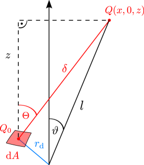
Figure 18: Geometry: $Q_{0}(r_{\mathrm{d}}\cos{\varphi},r_{\mathrm{d}}\sin{\varphi},0)$, $x=l\sin{\vartheta}$, $z=l\cos{\vartheta}$, $\mathrm{d}A=\mathrm{d}r_{\mathrm{d}}\,r_{\mathrm{d}}\,\mathrm{d}\varphi$.

In the following we derive an expression for the neutrino luminosities for an infinitesimal thin disk explicitly writing the constants $\hbar$ and $c$. For this purpose, we assume that the disk behaves like a blackbody source at a fixed temperature $T_{\nu}$ and take the neutrino number flux per unit energy per solid angle to be of Fermi-Dirac shape:

$$\mathcal{J}_{\nu}(E)=\dfrac{c}{(2\pi\hbar c)^{3}}\dfrac{E^{2}}{\mathrm{e}^{E/T_{\nu}}+1}.$$ (43)

The differential neutrino number flux per unit energy in a beam with differential solid angle $\mathrm{d}\Omega=\mathrm{d}A\cos(\Theta)/\delta^{2}$ at $Q(x,0,z)$ with a distance $l$ from the center of the disk is then given by (see Fig. 18):

$$\mathrm{d}\Phi_{\nu}(l,\vartheta,E)=\mathcal{J}_{\nu}(E)\dfrac{\mathrm{d}A\,\cos{\Theta}}{\delta^{2}},$$ (44)

where

$$\delta\equiv|\mathbf{Q}-\mathbf{Q}_{0}|=\sqrt{x^{2}+r_{\mathrm{d}}^{2}-2xr_{\mathrm{d}}\cos{\varphi}+z^{2}}$$ (45)

corresponds to the distance from the differential area $\mathrm{d}A$ to $Q$. The $\cos(\Theta)$-factor accounts for the fact that a distant observer at $Q$ only sees an effective area which accordingly reduces the flux. An integration over the disk yields the neutrino number flux per unit energy at $Q$:

$$\Phi_{\nu}(l,\vartheta,E)=\mathcal{J}_{\nu}(E)\int_{0}^{2\pi}\,\mathrm{d}\varphi\int_{0}^{R_{\nu}}\,\mathrm{d}r_{\mathrm{d}}r_{\mathrm{d}}\,\dfrac{\cos{\Theta}}{\delta^{2}}.$$ (46)

Using $\cos{\Theta}=z/\delta$ and $z=l\cos{\vartheta}$, it follows:

$$\Phi_{\nu}(l,\vartheta,E)=l\cos{\vartheta}\,\mathcal{J}_{\nu}(E)\int_{0}^{R_{\nu}}\,\mathrm{d}r_{\mathrm{d}}r_{\mathrm{d}}\int_{0}^{2\pi}\,\dfrac{\mathrm{d}\varphi}{\delta^{3}}.$$ (47)

For the explicit calculation, it is convenient Malkus et al. (2012) to introduce the quantities

$$L\equiv(x-r_{\mathrm{d}})^{2}+z^{2},\qquad M\equiv(x+r_{\mathrm{d}})^{2}+z^{2}$$ (48)

so that

$$\delta=\sqrt{\dfrac{L+M}{2}-\dfrac{M-L}{2}\cos{\varphi}}.$$ (49)

With the relation

$$\int_{0}^{2\pi}\,\dfrac{\mathrm{d}\varphi}{\delta^{3}}=\dfrac{4E\left(\sqrt{\frac{M-L}{M}}\right)}{L\sqrt{M}},$$ (50)

where

$$E(k)\equiv\int_{0}^{\pi/2}\,\mathrm{d}\theta\,\sqrt{1-k^{2}\sin^{2}{\theta}}$$ (51)

denotes Legendre’s complete elliptic integral of the second kind Olver et al. (2010), we find:

$$\Phi_{\nu}(l,\vartheta,E)=4l\cos{\vartheta}\,\mathcal{J}_{\nu}(E)\int_{0}^{R_{\nu}}\,\mathrm{d}r_{\mathrm{d}}\,r_{\mathrm{d}}\,\dfrac{E\left(\sqrt{\frac{M-L}{M}}\right)}{L\sqrt{M}}.$$ (52)

For an observer located at infinity, we compute the isotropized luminosity, i.e., the luminosity obtained by assuming an isotropically emitted flux:

$$L_{\nu}(\vartheta) =2\pi l^{2}\int_{0}^{\infty}\,\mathrm{d}E\,E\,\Phi_{\nu}(l,\vartheta,E)\biggr{\rvert}_{l\to\infty}$$ (53)

$$\begin{split}&=\dfrac{7}{120}\dfrac{\pi^{2}c}{(\hbar\,c)^{3}}\,T_{\nu}^{4}\,l^{3}\,\cos{\vartheta}\,\\ &\qquad\times\int_{0}^{R_{\nu}}\,\mathrm{d}r_{\mathrm{d}}\,r_{\mathrm{d}}\,\dfrac{E\left(\sqrt{\frac{M-L}{M}}\right)}{L\sqrt{M}}\biggr{\rvert}_{l\to\infty},\end{split}$$ (54)

where we used

$$\int_{0}^{\infty}\,\mathrm{d}E\,\dfrac{E^{3}}{\mathrm{e}^{E/T_{\nu}}+1}=\dfrac{7\pi^{4}}{120}T_{\nu}^{4}.$$ (55)

The asymptotic relation

$$\dfrac{E(\sqrt{\frac{M-L}{M}})}{L\sqrt{M}}=\dfrac{\pi}{2}\dfrac{1}{l^{3}}+\mathcal{O}(1/l^{5})\qquad(l\to\infty),$$ (56)

yields:

$$L_{\nu}(\vartheta) =\dfrac{7\pi}{4}\sigma_{\mathrm{SB}}\,T_{\nu}^{4}\,\cos{\vartheta}\,\int_{0}^{R_{\nu}}\,\mathrm{d}r_{\mathrm{d}}\,r_{\mathrm{d}}$$ (57)

$$=\dfrac{7\pi}{8}\sigma_{\mathrm{SB}}\,T_{\nu}^{4}\,R_{\nu}^{2}\,\cos{\vartheta},$$ (58)

where $\sigma_{\mathrm{SB}}\equiv\pi^{2}k_{\mathrm{B}}^{4}/(60\hbar^{3}c^{2})$ denotes the Stefan-Boltzmann constant.

Note that in the equations above, we considered a neutrino moving in the upward direction ($\cos{\vartheta}>0$). If we want to follow a neutrino moving downwards, we have to replace $\cos{\vartheta}$ by $-\cos{\vartheta}$, i.e. if $\frac{\pi}{2}<\vartheta<\pi$.

An integration over the upper hemisphere leads to the total neutrino luminosity:

$$L_{\nu} =\int_{0}^{1}\mathrm{d}(\cos{\vartheta})\,L_{\nu}(\vartheta)$$ (59)

$$=\dfrac{7\pi}{16}\sigma_{\mathrm{SB}}\,T_{\nu}^{4}\,R_{\nu}^{2}.$$ (60)

As an additional check, we also compute the total neutrino energy flux emitted from $\mathrm{d}A$:

$$\mathcal{F}_{\nu} =\int_{0}^{\infty}\mathrm{d}E\,E^{2}\,\mathcal{J}_{\nu}(E)\int\mathrm{d}\Omega\cos{\vartheta}$$ (61)

$$=\dfrac{7}{8}\dfrac{\pi}{120\hbar^{3}c^{2}}T_{\nu}^{4}\,2\pi\int_{0}^{1}\mathrm{d}(\cos{\vartheta})\cos{\vartheta}$$ (62)

$$=\dfrac{7}{16}\sigma_{\mathrm{SB}}T_{\nu}^{4}$$ (63)

and from that, we infer the total neutrino luminosity:

$$L_{\nu} =\pi R_{\nu}^{2}\mathcal{F}_{\nu}$$ (64)

$$=\dfrac{7\pi}{16}\sigma_{\mathrm{SB}}\,T_{\nu}^{4}\,R_{\nu}^{2}.$$ (65)

This expression agrees with the one derived above (Eq. (59)). For a simple estimate, it is useful to express this in the convenient form:

$$L_{\nu}\sim 15\times 10^{51}\,\mathrm{erg/s}\left(\dfrac{T_{\nu}}{3.4\,\mathrm{MeV}}\right)^{4}\left(\dfrac{R_{\nu}}{90\,\mathrm{km}}\right)^{2}$$ (66)

If we use the neutrino disks radii at $60\,\mathrm{ms}$ from Table 2 and the temperatures from Table 3, we obtain $L_{\nu_{e}}\approx 15\times 10^{51}\,\mathrm{erg/s}$, $L_{\bar{\nu}_{e}}\approx 33\times 10^{51}\,\mathrm{erg/s}$ and $L_{\nu_{x}}\approx 48\times 10^{51}\,\mathrm{erg/s}$. While the values for $L_{\nu_{e}}$ and $L_{\bar{\nu}_{e}}$ are compatible with the luminosities obtained in Perego et al. (2014), the value of $L_{\nu_{x}}$ is about 6 times larger.

Similarly, we compute the isotropized neutrino number luminosity:

$$L_{\mathrm{N},\nu}(\vartheta) =2\pi l^{2}\int_{0}^{\infty}\mathrm{d}E\,\Phi_{\nu}(l,\vartheta,E)\biggr{\rvert}_{l\to\infty}$$ (67)

$$=\dfrac{c}{(\hbar c)^{3}}\dfrac{F_{2}(0)}{4\pi}\cos{\vartheta}T_{\nu}^{3}R_{\nu}^{2}$$ (68)

and neutrino number luminosity:

$$L_{\mathrm{N},\nu} =\int_{0}^{1}\mathrm{d}(\cos\vartheta)\,L_{\mathrm{N},\nu}(\vartheta)$$ (69)

$$=\dfrac{c}{(\hbar c)^{3}}\dfrac{F_{2}(0)}{8\pi}T_{\nu}^{3}R_{\nu}^{2}.$$ (70)

In local thermal equilibrium we can relate the mean energy, defined Perego et al. (2014) via $\langle E_{\nu}\rangle=L_{\nu}/L_{\mathrm{N},\nu}$, to the effective temperature:

$$\langle E_{\nu}\rangle=\dfrac{F_{3}(0)}{F_{2}(0)}T_{\nu}.$$ (71)

However, we stress that the mechanism behind the spectra formation is rather demanding, since neutrinos decouple at different energy-dependent surfaces, and therefore our assumption of a thermal spectra which is determined by an effective temperature represents only a coarse approximation. In order to account for deviations from thermal equilibrium, one could examine different shapes of the spectral function similarly to studies that have been done in the context of core-collapse supernovae (e.g., Keil et al. (2003)).

If we multiply the neutrino number flux,

$$F_{\nu} =\int_{0}^{\infty}\mathrm{d}E\,\mathcal{J}_{\nu}(E)\int\mathrm{d}\Omega\,\cos{\vartheta}$$ (72)

$$=\dfrac{\pi c}{(2\pi\hbar c)^{3}}F_{2}(0)T_{\nu}^{3},$$ (73)

by the disk area $\pi R_{\nu}^{2}$, the same expression for the neutrino number luminosity $L_{\mathrm{N},\nu}=\pi R_{\nu}^{2}F_{\nu}$ as above is obtained:

$$L_{\mathrm{N},\nu}=\dfrac{c}{(\hbar c)^{3}}\dfrac{F_{2}(0)}{8\pi}T_{\nu}^{3}R_{\nu}^{2}.$$ (74)

Finally, we express the neutrino number flux in terms of the luminosity and mean neutrino energy:

$$F_{\nu}=\dfrac{1}{\pi R_{\nu}^{2}}\dfrac{L_{\nu}}{\langle E_{\nu}\rangle}.$$ (75)

and define the neutrino number flux per unit energy per solid angle as follows:

$$c\dfrac{\mathrm{d}^{2}n_{\nu}}{\mathrm{d}\Omega\mathrm{d}E}\equiv\dfrac{F_{\nu}}{\pi}f_{\nu}(E),$$ (76)

where

$$f_{\nu}(E)=\dfrac{1}{F_{2}(0)}\dfrac{1}{T_{\nu}^{3}}\dfrac{E^{2}}{\mathrm{e}^{E/T_{\nu}}+1}$$ (77)

denotes the normalized Fermi-Dirac distribution function with vanishing degeneracy parameter.

Consequently, the neutrino flux per unit energy corresponds to:

$$\Phi_{\nu}(E,x,z) =\int_{\Omega_{\nu}}\mathrm{d}\Omega\left(c\dfrac{\mathrm{d}^{2}n_{\nu}}{\mathrm{d}\Omega\mathrm{d}E}\right)$$ (78)

$$=\dfrac{F_{\nu}}{4\pi}f_{\nu}(E)\Omega_{\nu},$$ (79)

where the solid angle is given by

$$\Omega_{\nu}=4z\int_{R_{0}}^{R_{\nu}}\mathrm{d}r_{\mathrm{d}}r_{\mathrm{d}}\,\dfrac{E(\sqrt{\frac{M-L}{M}})}{L\sqrt{M}}.$$ (80)

We show a typical form of the solid angle in Fig. 19 along trajectory 2a.

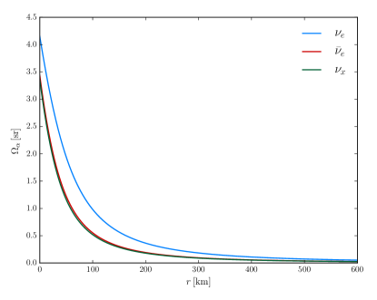
Figure 19: Solid angle for each neutrino species computed along trajectory 2a.

Since the neutrino disk radii for $\bar{\nu}_{e}$ and $\nu_{x}$ are similar, the difference in their corresponding solid angles is minor.

Appendix C Geometric factor

In this section we show the explicit structure of the geometric factor Eq. (30) used in the neutrino self-interaction Hamiltonian Eq. (31). An analytical calculation yields:

$$\int_{\Omega_{\nu_{\alpha}}}\mathrm{d}\Omega\,(1-\cos{\Theta_{\mathbf{p}\mathbf{p}^{\prime}}}) =\int_{\cos\theta_{\mathrm{max},\,\nu_{\alpha}}}^{+1}\mathrm{d}(\cos\theta)\int_{0}^{2\pi}\mathrm{d}\phi\,(1-\cos{\Theta_{\mathbf{p}\mathbf{p}^{\prime}}})$$ (81)

$$=\int_{R_{0}}^{R_{\nu_{\alpha}}}\mathrm{d}r_{\mathrm{d}}\int_{0}^{2\pi}\mathrm{d}\varphi\,|\mathrm{det}\,J|\,(1-\cos{\Theta_{\mathbf{p}\mathbf{p}^{\prime}}})$$ (82)

$$=z\int_{R_{0}}^{R_{\nu_{\alpha}}}\mathrm{d}r_{\mathrm{d}}\,r_{\mathrm{d}}\,\Gamma(r_{\mathrm{d}},\theta_{0},\phi_{0},x,z)$$ (83)

$$=:G_{\nu_{\alpha}}(\theta_{0},\phi_{0},x,z).$$ (84)

In the second step, we performed the previously described change of coordinates (Eqs. (20), (22), (25)) and introduced $\Gamma$ via:

$$\begin{split}\Gamma(r_{\mathrm{d}},\theta_{0},\phi_{0},x,z)\equiv\int_{0}^{2\pi}\mathrm{d}\varphi\left\{\dfrac{1}{\delta^{3}}\right.&\left.-\dfrac{z\cos\theta_{0}+x\sin\theta_{0}\cos\phi_{0}}{\delta^{4}}\right.\\ &\left.+r_{\mathrm{d}}\sin\theta_{0}\cos\phi_{0}\dfrac{\cos\varphi}{\delta^{4}}+r_{\mathrm{d}}\sin\theta_{0}\sin\phi_{0}\dfrac{\sin\varphi}{\delta^{4}}\right\},\end{split}$$ (85)

where $\delta$ is defined as in Eq. (49). In the single-trajectory approximation, the geometric factor $G_{\nu_{\alpha}}$ should be understood as an averaging over the angles. The explicit $\varphi$-integration in Eq. (85) yields:

$$\Gamma=\dfrac{4E\left(\sqrt{\frac{M-L}{M}}\right)}{L\sqrt{M}}-\dfrac{\pi\left\{(L+M)(z\cos\theta_{0}+x\sin\theta_{0}\cos\phi_{0})-4xr_{\mathrm{d}}^{2}\sin\theta_{0}\cos\phi_{0}\right\}}{(LM)^{3/2}},$$ (86)

where in the second step, the relation $M-L=4xr_{\mathrm{d}}$, with $M$ and $L$ defined in Eq. (48), was used and $E(k)$ denotes Legendre’s complete elliptic integral of the second kind Olver et al. (2010):

$$E(k)\equiv\int_{0}^{\pi/2}\mathrm{d}\theta\,\sqrt{1-k^{2}\sin^{2}{\theta}}.$$ (87)

Due to our definition of the angle $\phi$ that differs from the definition in Malkus et al. (2012), we note that $-\Gamma/2$ with the replacement $\phi_{0}\mapsto\pi-\phi_{0}$ corresponds to the geometric factor $C$ given in Malkus et al. (2012). Here, one also has to keep in mind the different convention used to denote the elliptic integral.

Appendix D Collected data

In the following table, we report a summary of published data concerning the neutrino luminosities and mean energies of a binary neutron star merger. We considered simulations of binary NS mergers Ruffert et al. (1997); Rosswog and Liebendörfer (2003); Rosswog et al. (2013); Sekiguchi et al. (2015); Foucart et al. (2016) or merger aftermaths Dessart et al. (2009); Metzger and Fernández (2014); Perego et al. (2014), including neutrino emission and characterized by the presence of a (possibly unstable) massive neutron star surrounded by a thick accretion disk. Since they run for very different amounts of time, for the merger simulations we choose the values when the luminosities have reached quasi-stationary values, while for the aftermath simulations the values close to the beginning of the calculation.

Table 7: Table with a summary of published data. We considered simulations of binary NS mergers or of their aftermath. In the former case, we report the time when the data were taken with respect to the beginning of the merger (in ms). In the latter case, we report data close to the beginning of the simulation. For all cases, we list the neutrino luminosities (in $10^{51}\,\mathrm{erg}\,\mathrm{s}^{-1}$), where for $\nu_{x}$, the values correspond to each single species, and, when available, the neutrino mean energies (in MeV, in the case of Foucart et al. (2016) the quantities provided are the rms energies).

Source	$t-t_{\mathrm{merger}}$	$L_{\nu_{e}}$	$L_{\bar{\nu}_{e}}$	$L_{\nu_{x}}$	$\langle E_{\nu_{e}}\rangle$	$\langle E_{\bar{\nu}_{e}}\rangle$	$\langle E_{\nu_{x}}\rangle$	Notes
Perego et al. (2014)	$-$	$15$	$32$	$8$	$10.6$	$15.3$	$17.3$	Grid, Newtonian, spectral leakage,
								HS(TM1) EOS, MNS + disk.
Ruffert et al. (1997)	$8$	$16$	$43$	$6$	$13$	$20$	$28$	Grid, Newtonian, gray leakage,
								LS(180) EOS, $1.65-1.65\,M_{\odot}$,
								no spin.
Rosswog and Liebendörfer (2003)	$18$	$45$	$130$	$25$	$9$	$15$	$20$	SPH, Newtonian, gray leakage,
								Shen EOS, $1.4-1.4\,M_{\odot}$,
								no spin.
Dessart et al. (2009)	$-$	$20$	$32$	$6$	$11$	$16$	$22$	Grid, Newtonian, MGFLD,
								Shen EOS, MNS + disk.
Rosswog et al. (2013)	$16$	$30$	$60$	$10$	$8$	$14.4$	$26.3$	SPH, Newtonian, gray leakage,
								Shen EOS, $1.3-1.4\,M_{\odot}$,
								no spin.
Metzger and Fernández (2014)	$-$	$55$	$45$	$-$	$12$	$15$	$-$	Grid, Newtonian, gray leakage,
								Timmes & Swesty EOS,
								MNS + disk.
Sekiguchi et al. (2015)	$30$	$120$	$200$	$15$	$-$	$-$	$-$	Grid, GR, gray GR leakage +
								moment formalism for
								free streaming $\nu$’s,
								HS(TM1) EOS, $1.35-1.35\,M_{\odot}$,
								no spin.
Sekiguchi et al. (2015)	$30$	$100$	$150$	$10$	$-$	$-$	$-$	Grid, GR, $\nu$’s as above,
								HS(DD2) EOS, $1.35-1.35\,M_{\odot}$,
								no spin.
Sekiguchi et al. (2015)	$10$	$175$	$280$	$100$	$-$	$-$	$-$	Grid, GR, $\nu$ as above,
								SFHo EOS, $1.35-1.35\,M_{\odot}$,
								no spin.
Foucart et al. (2016)	$10$	$120$	$210$	$30$	$13$	$20$	$26$	Grid, GR, gray GR leakage,
								LS(220) EOS, $1.2-1.2\,M_{\odot}$,
								no spin.
Foucart et al. (2016)	$10$	$160$	$220$	$22.5$	$13$	$20$	$24$	Grid, GR, gray GR leakage,
								HS(DD2) EOS, $1.2-1.2\,M_{\odot}$,
								no spin.
Foucart et al. (2016)	$10$	$190$	$300$	$55$	$14$	$21$	$29$	Grid, GR, gray GR leakage,
								SFHo EOS, $1.2-1.2\,M_{\odot}$,
								no spin.
Foucart et al. (2016)	$10$	$60$	$210$	$70$	$13$	$20$	$26$	Grid, GR, gray GR M1,
								LS(220) EOS, $1.2-1.2\,M_{\odot}$,
								no spin.

Appendix E Matter-neutrino resonance locations

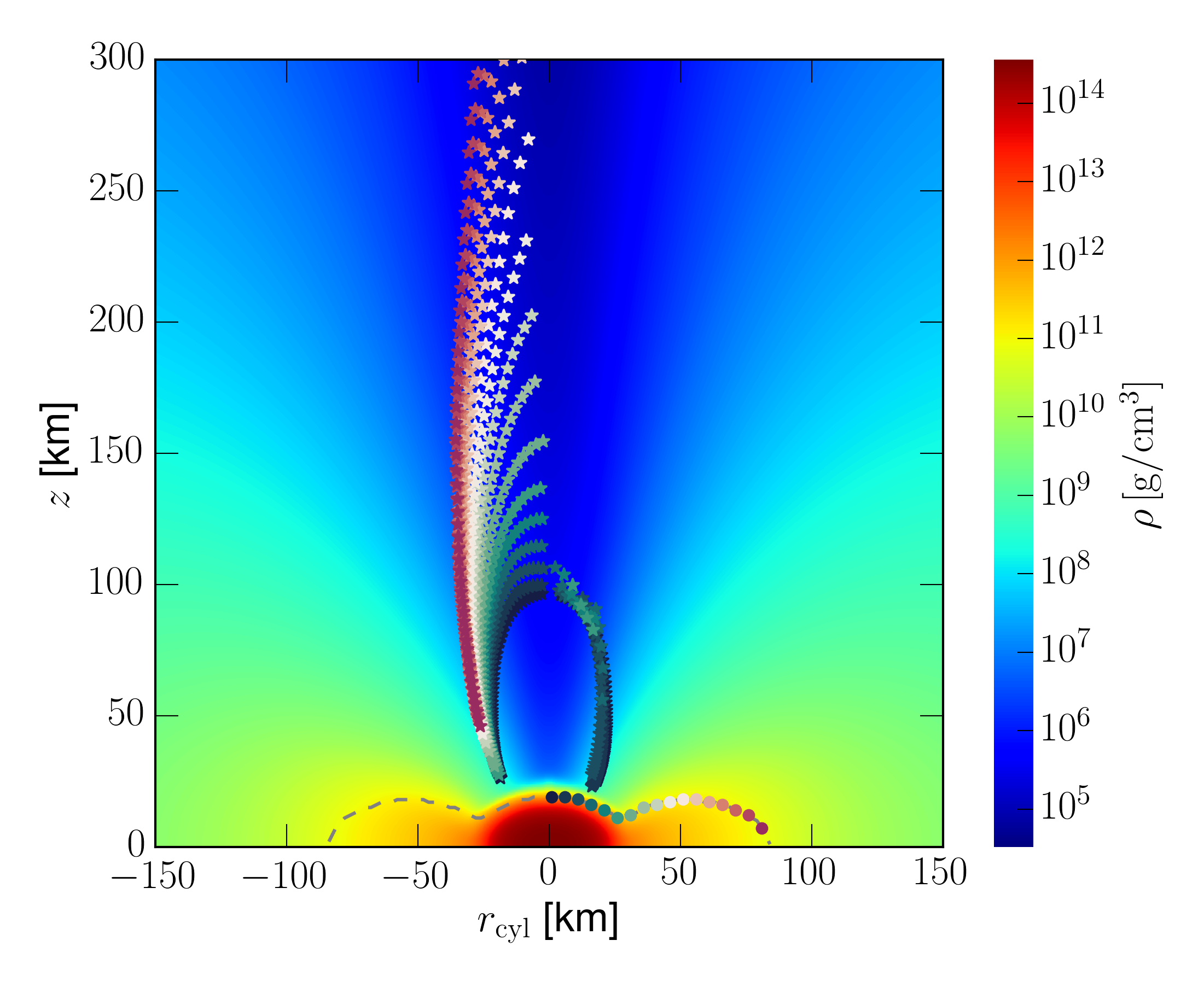
Figure 20: Cancellation points ($\star$), i.e. points where $\lambda+\mu\approx 0$, for several trajectories above the BNS merger remnant. The emission points are represented by $\bullet$. Emission and cancellation points with the same color refer to a single trajectory. Points where the crossing starts dominated by matter are excluded. Color coded is the density of matter.

The initial conditions employed in this work are close to the ones used by Zhu et al. (2016), who also investigated the flavor evolution in BNS mergers. This allows a close comparison between the two different works. In particular, we compute the locations above the remnant where MNR occurs and compare with the results reported by Zhu et al. (2016) in their figure 6. These locations can be identified as cancellation points, i.e., points where the unoscillated neutrino self-interaction potential cancels with the matter potential along a specific trajectory, $\lambda+\mu\approx 0$. In Fig. 20, we represent the cancellation points for several different trajectories starting from the disk. The emerging picture suggests that the resonances for neutrinos originating from one side of the disk are preferably located at the edge of the funnel. Neutrinos emerging from the MNS will all encounter MNR, probably with some flavor transformations depending on the adiabaticity. In contrast, neutrinos emitted from the disk will only encounter MNR if they propagate through the central regions of the funnel, where the matter density is relatively low. Remarkably, this picture is qualitatively consistent with the results found in Zhu et al. (2016). Nevertheless, quantitative differences between the two works can be present and traced back to the different approaches used in the two works to model the radiation field outside the neutrino surfaces. On the one hand, we have assumed a thin disk model, emitting thermal radiation from a spectrally averaged, single-temperature neutrino surface. On the other hand, Zhu et al. (2016) used an energy-dependent leakage scheme and a ray-tracing algorithm to model the emission from a finite size, thick disk. They also take explicitly into account radiation damping effects outside the neutrino surfaces.

References

- Abbott et al. (2016) B. P. Abbott et al. (LIGO Scientific Collaboration and Virgo Collaboration), Phys. Rev. Lett. 116, 061102 (2016).
- Rosswog (2015) S. Rosswog, Int. J. Mod. Phys. D24, 1530012 (2015).
- Faber and Rasio (2012) J. A. Faber and F. A. Rasio, Living Rev. Rel. 15, 8 (2012).
- Lattimer and Schramm (1974) J. M. Lattimer and D. N. Schramm, ApJL. 192, L145 (1974).
- Eichler et al. (1989) D. Eichler, M. Livio, T. Piran, and D. N. Schramm, Nature 340, 126 (1989).
- Paczynski (1986) B. Paczynski, ApJ 308, L43 (1986).
- Nakar (2007) E. Nakar, Phys. Rept. 442, 166 (2007).
- Pontecorvo (1957) B. Pontecorvo, Sov. Phys. JETP 6, 429 (1957), [Zh. Eksp. Teor. Fiz.33,549(1957)].
- Pontecorvo (1958) B. Pontecorvo, Sov. Phys. JETP 7, 172 (1958), [Zh. Eksp. Teor. Fiz.34,247(1957)].
- Pontecorvo (1968) B. Pontecorvo, Sov. Phys. JETP 26, 984 (1968), [Zh. Eksp. Teor. Fiz.53,1717(1967)].
- Fukuda et al. (1998) Y. Fukuda et al. (Super-Kamiokande Collaboration), Phys. Rev. Lett. 81, 1562 (1998).
- Ahmad et al. (2002) Q. R. Ahmad et al. (SNO Collaboration), Phys. Rev. Lett. 89, 011301 (2002).
- Wolfenstein (1978) L. Wolfenstein, Phys. Rev. D 17, 2369 (1978).
- Mikheyev and Smirnov (1986) S. Mikheyev and A. Smirnov, Il Nuovo Cim. C 9, 17 (1986).
- Fuller et al. (1987) G. M. Fuller, R. W. Mayle, J. R. Wilson, and D. N. Schramm, Astrophys. J. 322, 795 (1987).
- Nötzold and Georg (1988) D. Nötzold and R. Georg, Nucl. Phys. B 307, 924 (1988).
- Pantaleone (1992a) J. Pantaleone, Phys. Rev. D 46, 510 (1992a).
- Pantaleone (1992b) J. Pantaleone, Phys. Lett. B 287, 128 (1992b).
- Chakraborty et al. (2016) S. Chakraborty, R. Hansen, I. Izaguirre, and G. Raffelt, Nucl. Phys. B (2016), 10.1016/j.nuclphysb.2016.02.012.
- Duan (2015) H. Duan, Int. J. Mod. Phys. E 24, 1541008 (2015).
- Duan et al. (2010) H. Duan, G. M. Fuller, and Y.-Z. Qian, Annu. Rev. Nucl. Part. Sci. 60, 569 (2010).
- Malkus et al. (2012) A. Malkus, J. P. Kneller, G. C. McLaughlin, and R. Surman, Phys. Rev. D 86, 085015 (2012).
- Malkus et al. (2014) A. Malkus, A. Friedland, and G. C. McLaughlin, ArXiv e-prints (2014), arXiv:1403.5797 [hep-ph] .
- Malkus et al. (2016) A. Malkus, G. C. McLaughlin, and R. Surman, Phys. Rev. D 93, 045021 (2016).
- Wu et al. (2016a) M.-R. Wu, H. Duan, and Y.-Z. Qian, Phys. Lett. B 752, 89 (2016a).
- Väänänen and McLaughlin (2016) D. Väänänen and G. C. McLaughlin, Phys. Rev. D 93, 105044 (2016).
- Vlasenko et al. (2014a) A. Vlasenko, G. M. Fuller, and V. Cirigliano, (2014a), arXiv:1406.6724 [astro-ph.HE] .
- Wu et al. (2016b) M.-R. Wu, G. Martinez-Pinedo, and Y.-Z. Qian, Proceedings, 13th International Symposium on Origin of Matter and Evolution of the Galaxies (OMEG2015), EPJ Web Conf. 109, 06005 (2016b).
- Stapleford et al. (2016) C. J. Stapleford, D. J. Väänänen, J. P. Kneller, G. C. McLaughlin, and B. T. Shapiro, (2016), arXiv:1605.04903 [hep-ph] .
- Duan et al. (2006) H. Duan, G. M. Fuller, J. Carlson, and Y.-Z. Qian, Phys. Rev. D 74, 105014 (2006).
- Qian and Fuller (1995) Y.-Z. Qian and G. M. Fuller, Phys. Rev. D 51, 1479 (1995).
- Fogli et al. (2007) G. L. Fogli, E. Lisi, A. Marrone, and A. Mirizzi, JCAP 0712, 010 (2007), 0707.1998 .
- Dasgupta et al. (2009) B. Dasgupta, A. Dighe, G. G. Raffelt, and A. Y. Smirnov, Phys. Rev. Lett. 103, 051105 (2009).
- Duan and Friedland (2011) H. Duan and A. Friedland, Phys. Rev. Lett. 106, 091101 (2011).
- Perego et al. (2014) A. Perego, S. Rosswog, R. M. Cabezón, O. Korobkin, R. Käppeli, A. Arcones, and M. Liebendörfer, MNRAS 443, 3134 (2014).
- Hotokezaka et al. (2013) K. Hotokezaka, K. Kiuchi, K. Kyutoku, T. Muranushi, Y.-i. Sekiguchi, M. Shibata, and K. Taniguchi, Phys. Rev. D88, 044026 (2013).
- Baumgarte et al. (2000) T. W. Baumgarte, S. L. Shapiro, and M. Shibata, Astrophys. J. 528, L29 (2000).
- Kaplan et al. (2014) J. D. Kaplan, C. D. Ott, E. P. O’Connor, K. Kiuchi, L. Roberts, and M. Duez, Astrophys. J. 790, 19 (2014).
- Perego et al. (2016) A. Perego, R. M. Cabezón, and R. Käppeli, Astrophys. J. Suppl. 223, 22 (2016), arXiv:1511.08519 [astro-ph.IM] .
- Duncan et al. (1986) R. C. Duncan, S. L. Shapiro, and I. Wasserman, ApJ 309, 141 (1986).
- Qian and Woosley (1996) Y. Z. Qian and S. E. Woosley, Astrophys. J. 471, 331 (1996).
- Just et al. (2015) O. Just, A. Bauswein, R. A. Pulpillo, S. Goriely, and H.-T. Janka, MNRAS 448, 541 (2015).