Micromechanics and dislocation theory in anisotropic elasticity

Abstract

In this work, dislocation master-equations valid for anisotropic materials are derived in terms of kernel functions using the framework of micromechanics. The second derivative of the anisotropic Green tensor is calculated in the sense of generalized functions and decomposed into a sum of a $1/R^{3}$-term plus a Dirac $\delta$-term. The first term is the so-called “Barnett-term” and the latter is important for the definition of the Green tensor as fundamental solution of the Navier equation. In addition, all dislocation master-equations are specified for Somigliana dislocations with application to 3D crack modeling. Also the interior Eshelby tensor for a spherical inclusion in an anisotropic material is derived as line integral over the unit circle.

Keywords: Dislocations, anisotropic elasticity, Green tensor, derivatives, micromechanics, Eshelby tensor.

1 Introduction

The fields of defects such as dislocations, cracks, and inclusions play an important role in determining the physical properties of solids. Especially, dislocations play an important role as the elementary defect causing plasticity and hardening in crystals [Kröner, 1958; Lardner, 1974]. The micromechanics of isotropic inclusions and anisotropic inclusions based on Green tensors is an active and important research field of the so-called eigenstrain theory [Mura, 1987; Buryachenko, 2007; Li and Wang, 2008]. Another application of the eigenstrain theory is the dislocation theory [Mura, 1987; Li and Wang, 2008]. Nowadays, the dislocation fields are important for computer simulations of dislocation dynamics, dislocation based plasticity, and dislocation based fracture mechanics. The classical field theory of dislocations (theory of internal stresses) is the theory of incompatible anisotropic elasticity where a prescribed plastic distortion plays the role of the eigendistortion. In dislocation theory, the nonuniform plastic distortion gives rise to a measurable amount of incompatibility called the dislocation density tensor [Kröner, 1958, 1981; Lardner, 1974]. The prescribed plastic distortion and dislocation density tensors are the sources for the elastic fields of dislocations. In the framework of field theory of anisotropic elasticity, the Green tensor and its derivatives play an essential role to determine the elastic fields caused by a dislocation in an anisotropic body.

In this work, we provide anisotropic dislocation master-formulas based on the anisotropic Green tensor and related tensors for arbitrary dislocation densities and plastic distortions including Volterra and Somigliana dislocations in the framework of eigenstrain theory. Volterra dislocations are realized as dislocations in crystals where the Burgers vector is fixed by the crystal lattice. Nowadays, Somigliana dislocations play a role as crack dislocations where the displacement jump (Burgers vector) is variable [Eshelby, 1982; Hills et al., 1996]. One aim of this work is to give a necessary set of dislocation master-equations for Somigliana dislocations in an anisotropic medium of infinite extent needed for numerical simulations of three-dimensional (3D) crack modeling.

The paper is organized into six sections. In Sec. 2, microelasticity and anisotropic elasticity with the Green tensors, their derivatives, related kernel functions, related tensors, the dislocation master-equations for arbitrary prescribed plastic distortion, and dislocation density are introduced and derived. In Sec. 3, the dislocation master-equations are specified for Somigliana dislocations. In Sec. 4, the relation to 3D crack modeling based on Somigliana dislocations is given and reviewed. In Sec. 5, based on the second derivative of the anisotropic Green tensor, the Eshelby tensor for a spherical inclusion in an anisotropic material is given. Finally, in Sec. 6, the conclusions are given. Technical details are given in two Appendices.

2 Dislocations in anisotropic elasticity

In this Section, we derive all the necessary dislocation master-equations for arbitrary plastic distortion and dislocation density tensors in an anisotropic material using the eigenstrain theory. We use the Green tensor method since it provides a convenient framework to calculate the fields of dislocations in anisotropic media. We consider linear elastic anisotropic bodies which are infinite in extent.

2.1 Basic framework

First of all, we review the general dislocation master-equations which are valid in linear anisotropic elasticity as well as in isotropic elasticity. The static equilibrium condition for self-stresses reads

$$\sigma_{ij,j}=0\,,$$ (1)

where $\bm{\sigma}$ is the symmetric stress tensor. We use the indicial comma notation to indicate spatial differentiation: $\partial_{j}$ is indicated by the subscript notation “$,j$”. For the general anisotropic case, the stress tensor is related to the elastic distortion tensor $\bm{\beta}$ by Hooke’s law

$$\sigma_{ij}=C_{ijkl}\beta_{kl}\,,$$ (2)

where $C_{ijkl}$ is the fourth-rank tensor of elastic constants. The tensor $C_{ijkl}$ satisfies the symmetry conditions

$$C_{ijkl}=C_{klij}=C_{jikl}=C_{ijlk}\,.$$ (3)

According to Kröner [1958], the gradient of the displacement vector $\bm{u}$, which is the total distortion tensor, can be decomposed into the elastic distortion tensor $\bm{\beta}$ and the plastic distortion tensor (or eigendistortion tensor) $\bm{\beta}^{\mathrm{P}}$

$$u_{i,j}=\beta_{ij}+\beta_{ij}^{\mathrm{P}}\,.$$ (4)

The dislocation density tensor $\bm{\alpha}$ is defined in terms of the plastic distortion tensor [Kröner, 1958, 1981]

$$\alpha_{ij}=-\epsilon_{jkl}\beta^{{\mathrm{P}}}_{il,k}\,$$ (5)

or in terms of the elastic distortion tensor

$$\alpha_{ij}=\epsilon_{jkl}\beta_{il,k}\,,$$ (6)

where $\epsilon_{jkl}$ is the Levi-Civita tensor or permutation tensor. The dislocation density tensor satisfies the dislocation Bianchi identity

$$\alpha_{ij,j}=0\,,$$ (7)

which has the meaning that dislocations cannot end inside the body.

2.2 General dislocation master-equations

If we substitute Eqs. (2) and (4) into Eq. (1), we obtain an inhomogeneous Navier equation for the displacement vector

$$C_{ijkl}u_{k,lj}=C_{ijkl}\beta_{kl,j}^{\mathrm{P}}\,,$$ (8)

where the inhomogeneous part (or source part) is given by the plastic distortion tensor $\bm{\beta}^{\mathrm{P}}$. The Green tensor of the Navier equation (elliptic partial differential equation of second order) is defined by

$$C_{ijkl}G_{km,lj}({\bm{x}}-{\bm{x}}^{\prime})+\delta_{im}\delta({\bm{x}}-{\bm{x}}^{\prime})=0\,$$ (9)

and is the fundamental solution of the Navier operator $C_{ijkl}\partial_{j}\partial_{l}$. $\delta_{im}$ is the Kronecker delta tensor and $\delta({\bm{x}}-{\bm{x}}^{\prime})$ is the three-dimensional Dirac delta function which is zero everywhere, except at point ${\bm{x}}={\bm{x}}^{\prime}$. The Green tensor $G_{ij}({\bm{x}}-{\bm{x}}^{\prime})$ satisfies the symmetry relations [Bacon et al., 1979]

$$G_{ij}({\bm{x}}-{\bm{x}}^{\prime})=G_{ij}({\bm{x}}^{\prime}-{\bm{x}})=G_{ji}({\bm{x}}-{\bm{x}}^{\prime})\,$$ (10)

and

$$G_{ij,k}({\bm{x}}-{\bm{x}}^{\prime})=-G_{ij,k^{\prime}}({\bm{x}}-{\bm{x}}^{\prime})=-G_{ij,k}({\bm{x}}^{\prime}-{\bm{x}})$$ (11)

$$G_{ij,kl}({\bm{x}}-{\bm{x}}^{\prime})=G_{ij,k^{\prime}l^{\prime}}({\bm{x}}-{\bm{x}}^{\prime})=-G_{ij,kl^{\prime}}({\bm{x}}-{\bm{x}}^{\prime})=G_{ij,kl}({\bm{x}}^{\prime}-{\bm{x}})\,,$$ (12)

where the unprimed subscripts denote partial differentiation with respect to ${\bm{x}}$ and primed subscripts denote differentiation with respect to ${\bm{x}}^{\prime}$. Using the Green tensor, the solution of Eq. (8) is the convolution of the Green tensor with the plastic distortion tensor $\bm{\beta}^{\mathrm{P}}$

$$u_{i}=-C_{jkln}G_{ij,k}*\beta_{ln}^{\mathrm{P}}\,,$$ (13)

where $*$ denotes the spatial convolution. Eq. (13) is the generalized Volterra formula for an arbitrary plastic distortion.

The gradient of Eq. (13) gives

$$u_{i,m} =-C_{jkln}G_{ij,km}*\beta_{ln}^{\mathrm{P}}\,.$$ (14)

The elastic distortion is obtained from Eq. (4) as

$$\beta_{im}=-C_{jkln}G_{ij,km}*\beta_{ln}^{\mathrm{P}}-\beta_{im}^{\mathrm{P}}\,.$$ (15)

Defining the kernel $\bm{R}$ [Simmons and Bullough, 1970]

$$R_{imln}({\bm{x}}-{\bm{x}}^{\prime}) :=-C_{jkln}G_{ij,km^{\prime}}({\bm{x}}-{\bm{x}}^{\prime})+\delta_{il}\delta_{mn}\delta({\bm{x}}-{\bm{x}}^{\prime})$$

$$\ =C_{jkln}G_{ij,km}({\bm{x}}-{\bm{x}}^{\prime})+\delta_{il}\delta_{mn}\delta({\bm{x}}-{\bm{x}}^{\prime})\,,$$ (16)

Eq. (15) reduces to

$$\beta_{im}=-R_{imln}*\beta_{ln}^{\mathrm{P}}\,.$$ (17)

Using Eq. (2), the stress tensor reads

$$\sigma_{pq}=-C_{pqim}\big{(}C_{jkln}G_{ij,km}*\beta_{ln}^{\mathrm{P}}+\beta_{im}^{\mathrm{P}}\big{)}\,,$$ (18)

which can be simply written

$$\sigma_{pq}=-S_{pqln}*\beta_{ln}^{\mathrm{P}}\,,$$ (19)

where the kernel $\bm{S}$ is defined by (see also Simmons and Bullough [1970]; Kunin [1983])

$$S_{pqln}({\bm{x}}-{\bm{x}}^{\prime}) :=C_{pqim}R_{imln}({\bm{x}}-{\bm{x}}^{\prime})$$

$$\ =C_{pqim}\big{(}C_{jkln}G_{ij,km}({\bm{x}}-{\bm{x}}^{\prime})+\delta_{il}\delta_{mn}\delta({\bm{x}}-{\bm{x}}^{\prime})\big{)}\,.$$ (20)

$S_{pqln}({\bm{x}}-{\bm{x}}^{\prime})$ is symmetric in the indices $pq$ and $ln$ and possesses the additional symmetry properties

$$S_{pqln}({\bm{x}}-{\bm{x}}^{\prime})=S_{pqln}({\bm{x}}^{\prime}-{\bm{x}})=S_{lnpq}({\bm{x}}-{\bm{x}}^{\prime})$$ (21)

following from the symmetries (3) and (10). Eqs. (15) and (18) give the elastic distortion and the stress, respectively, for a prescribed plastic distortion (or eigendistortion). Note that in elasticity, the kernels $\bm{R}$ and $\bm{S}$ possess $1/R^{3}$- and $\delta$-singularities. Formulas like (15) and (18) are also known in the Eshelby-Mura eigenstrain theory and micromechanics (see, e.g., Mura [1987]; Li and Wang [2008]). In micromechanics, the second derivative of the Green tensor is more often used than the Green tensor and the first derivative of the Green tensor.

On the other hand, Eq. (14) can be rewritten as

$$u_{i,m} =-C_{jkln}G_{ij,k}*\beta_{ln,m}^{\mathrm{P}}$$

$$=-C_{jkln}G_{ij,k}*\big{(}\beta_{lm,n}^{\mathrm{P}}+\epsilon_{nmr}\alpha_{lr}\big{)}$$

$$=-C_{jkln}G_{ij,kn}*\beta_{lm}^{\mathrm{P}}-\epsilon_{nmr}C_{jkln}G_{ij,k}*\alpha_{lr}$$

$$=\beta_{im}^{\mathrm{P}}+\epsilon_{mnr}C_{jkln}G_{ij,k}*\alpha_{lr}\,,$$ (22)

which gives now for the elastic distortion tensor the so-called Mura-Willis formula for an arbitrary dislocation density

$$\beta_{im}=\epsilon_{mnr}C_{jkln}G_{ij,k}*\alpha_{lr}\,.$$ (23)

Defining the kernel $\bm{D}$ [Simmons and Bullough, 1970]

$$D_{imlr}({\bm{x}}-{\bm{x}}^{\prime}):=\epsilon_{mnr}C_{jkln}G_{ij,k}({\bm{x}}-{\bm{x}}^{\prime})$$ (24)

which obeys the symmetry properties

$$D_{imlr}({\bm{x}}-{\bm{x}}^{\prime})=-D_{imlr}({\bm{x}}^{\prime}-{\bm{x}})=-D_{irlm}({\bm{x}}-{\bm{x}}^{\prime})\,,$$ (25)

Eq. (23) simply reads

$$\beta_{im}=D_{imlr}*\alpha_{lr}\,.$$ (26)

Substituting Eq. (23) into Eq. (2), the stress tensor reduces to

$$\sigma_{pq}=C_{pqim}\epsilon_{mnr}C_{jkln}G_{ij,k}*\alpha_{lr}$$ (27)

which is the generalized Peach-Koehler stress formula for an arbitrary dislocation density. Eq. (27) can be simply written as follows

$$\sigma_{pq}=M_{pqlr}*\alpha_{lr}$$ (28)

if we introduce the kernel $\bm{M}$

$$M_{pqlr}({\bm{x}}-{\bm{x}}^{\prime}) :=C_{pqim}D_{imlr}({\bm{x}}-{\bm{x}}^{\prime})$$

$$\ =C_{pqim}\epsilon_{mnr}C_{jkln}G_{ij,k}({\bm{x}}-{\bm{x}}^{\prime})$$ (29)

which possesses the symmetry properties

$$M_{pqlr}({\bm{x}}-{\bm{x}}^{\prime})=-M_{pqlr}({\bm{x}}^{\prime}-{\bm{x}})=M_{qplr}({\bm{x}}-{\bm{x}}^{\prime})\,.$$ (30)

Note that the curl of the kernels $\bm{D}$ and $\bm{M}$ leads to the kernels $\bm{R}$ and $\bm{S}$, respectively

$$\epsilon_{qrp}D_{imlr,p}=R_{imlq}$$ (31)

$$\epsilon_{qrp}M_{imlr,p}=S_{imlq}\,.$$ (32)

Thus, Eqs. (26) and (28) give the elastic distortion and the stress, respectively, for a prescribed dislocation density. Note that in elasticity, the kernels $\bm{D}$ and $\bm{M}$ possess a $1/R^{2}$-singularity. Thus, Eqs. (26) and (28) are less singular than Eqs. (15) and (18). In dislocation theory, the first derivative of the Green tensor is of primary importance.

From Eq. (4), we can derive the following Poisson equation for the displacement vector

$$\Delta u_{i}=\beta_{ij,j}+\beta_{ij,j}^{\mathrm{P}}\,,$$ (33)

where $\Delta$ is the Laplace operator. Using the three-dimensional Green function of the Laplace operator [Vladimirov, 1971]

$$G^{\Delta}=-\frac{1}{4\pi R}\,,\qquad\Delta G^{\Delta}=\delta({\bm{x}}-{\bm{x}}^{\prime})\,,$$ (34)

where $R=|{\bm{x}}-{\bm{x}}^{\prime}|$ is the distance between field and source points, the solution of Eq. (33) can be written as convolution

$$u_{i}=\big{(}\beta_{ij,j}+\beta_{ij,j}^{\mathrm{P}}\big{)}*G^{\Delta}$$ (35)

and finally

$$u_{i}=G^{\Delta}_{,j}*\beta^{\mathrm{P}}_{ij}+\beta_{ij,j}*G^{\Delta}\,.$$ (36)

Substituting the Mura-Willis equation (23) into Eq. (36), we obtain

$$u_{i} =G^{\Delta}_{,j}*\beta^{\mathrm{P}}_{ij}+\epsilon_{mnr}C_{jkln}G_{ij,km}*\alpha_{lr}*G^{\Delta}$$

$$=G^{\Delta}_{,j}*\beta^{\mathrm{P}}_{ij}+\epsilon_{mnr}C_{jkln}G_{ij,km}*G^{\Delta}*\alpha_{lr}\,.$$ (37)

The double convolution can be reduced to a single one by defining the $\bm{F}$-tensor introduced by Kirchner [1984] (see also Lazar and Kirchner [2013])

$$F_{mkij}:=-G_{ij,km}*G^{\Delta}\,.$$ (38)

Thus, the $\bm{F}$-tensor is the convolution of the second derivative of the Green tensor with the Green function of the Laplace operator. It satisfies a tensorial Poisson equation

$$\Delta F_{mkij}=-G_{ij,km}\,.$$ (39)

Moreover, the following relationships hold

$$F_{mkij,m}+G_{ij,k}=0\,,\qquad F_{mkij,k}+G_{ij,m}=0\,,$$ (40)

$$F_{mkij,mk}+\Delta G_{ij}=0\,,$$ (41)

and

$$\delta_{mk}F_{mkij}=-G_{ij}\,.$$ (42)

$F_{mkij}$ obeys the symmetry properties

$$F_{mkij}=F_{kmij}=F_{mkji}\,,$$ (43)

and

$$F_{mkij}({\bm{x}}-{\bm{x}}^{\prime})=F_{mkij}({\bm{x}}^{\prime}-{\bm{x}})\,.$$ (44)

Combining Eqs. (9) and (39), we obtain

$$\Delta C_{iklm}F_{mkij}=-C_{iklm}G_{ij,km}=\delta_{jl}\delta(\bm{r}-\bm{r}^{\prime})$$ (45)

and from (38) with (9), we get

$$C_{iklm}F_{mkij}=-C_{iklm}G_{ij,km}*G^{\Delta}=\delta_{jl}G^{\Delta}\,.$$ (46)

Using the $\bm{F}$-tensor, the displacement is given by the generalized Burgers equation

$$u_{i} =G^{\Delta}_{,j}*\beta^{\mathrm{P}}_{ij}-\epsilon_{mnr}C_{jkln}F_{mkij}*\alpha_{lr}\,.$$ (47)

Eq. (47) gives a decomposition of the displacement vector into a purely geometric part convoluted with a prescribed plastic distortion and a part depending on the elastic constants convoluted with the dislocation density tensor.

All the given equations are valid for anisotropic elasticity as well as isotropic elasticity. Only the corresponding Green tensor and $\bm{F}$-tensor have to be substituted. They are given for any plastic distortion and dislocation density, that means they are valid for Volterra dislocations as well as for Somigliana dislocations (see Sec. 3).

2.3 Green tensor, $\bm{F}$-tensor, their derivatives and corresponding kernels for arbitrary anisotropic elasticity

For anisotropic elasticity, the Green tensor reads [Lifshitz and Rosenzweig, 1947; Synge, 1957; Barnett, 1972]

$$G_{ij}(\bm{R}) =\frac{1}{8\pi^{2}R}\,\int_{0}^{2\pi}(nCn)_{ij}^{-1}\,\text{d}\phi\,,$$ (48)

where $\bm{n}=\bm{\kappa}(\pi/2,\phi)$ and $\bm{R}={\bm{x}}-{\bm{x}}^{\prime}$. The second rank symmetric tensor, sometimes called Christoffel stiffness tensor, is defined as

$$(nCn)_{ij}=n_{k}C_{ikjl}n_{l}\,$$ (49)

and the inverse tensor $(nCn)^{-1}_{ij}$ of $(nCn)_{ij}$ is defined by the property

$$(nCn)^{-1}_{ip}\,(nCn)_{pj}=(nCn)_{ip}\,(nCn)_{pj}^{-1}=\delta_{ij}\,.$$ (50)

Here $\bm{\kappa}=\bm{k}/k$ with $k=|\bm{k}|$ is a unit vector in the Fourier space with $\bm{\kappa}=\bm{\kappa}(\theta,\phi)$. Eq. (48) is the famous Lifshitz-Rosenzweig-Synge-Barnett representation of the Green tensor for arbitrary anisotropy which is a line integral along the unit circle in the plane orthogonal to $\bm{R}$ (see Fig. 1). Thus, $\bm{n}$ is perpendicular to $\bm{R}$, namely $\bm{n}\cdot\bm{R}=0$.

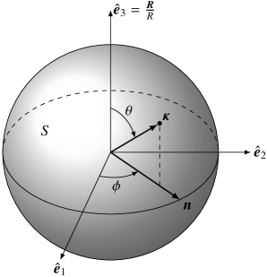
Figure 1: The unit sphere in Fourier space. The unit vector $\bm{\kappa}(\theta,\phi)$ is defined by the azimuth angle $\phi$, and the zenith angle $\theta$ and its projection $\bm{n}=\bm{\kappa}(\pi/2,\phi)$ is measured from the axis $\hat{\bm{e}}_{3}=\bm{R}/R$.

The first derivative of the Green tensor (48) is given by (see Appendix B and Barnett [1972]; Bacon et al. [1979])

$$G_{ij,k}({\bm{R}})=-\frac{1}{8\pi^{2}R^{2}}\,\int_{0}^{2\pi}\Big{(}\tau_{k}(nCn)_{ij}^{-1}-n_{k}F_{ij}\Big{)}\,{\mathrm{d}}\phi\,$$ (51)

with the unit vector

$${\bm{\tau}}=\frac{{\bm{R}}}{R}$$ (52)

and

$$F_{ij}=(nCn)_{ip}^{-1}\big{[}(nC\tau)_{pq}+(\tau Cn)_{pq}\big{]}(nCn)_{qj}^{-1}\,.$$ (53)

The $\bm{F}$-tensor reads [Kirchner, 1984; Lazar and Kirchner, 2013]

$$F_{mkij}(\bm{R}) =-\frac{1}{8\pi^{2}R}\,\int_{0}^{2\pi}n_{m}n_{k}\,(nCn)_{ij}^{-1}\,\text{d}\phi\,,$$ (54)

which is also a line integral along the unit circle in the plane orthogonal to $\bm{R}$. Using Eqs. (54) and (50), it can be easily seen that the relation (46) is fulfilled, and using Eqs.  (54), (50) and (34), it can be easily seen that the relation (45) is satisfied.

An important similarity is that both $G_{ij}(\bm{R})$ and $F_{mkij}(\bm{R})$ have a $1/R$-singularity and their Fourier transforms $\hat{G}_{ij}(\bm{k})$ and $\hat{F}_{mkij}(\bm{k})$ are proportional to $k^{-2}$. On the other hand, the second derivative of the Green tensor, $G_{ij,km}(\bm{R})=-\Delta F_{mkij}(\bm{R})$, is a generalized function (distribution), whose Fourier transform, $k_{k}k_{m}\hat{G}_{ij}(\bm{k})=-k^{2}\hat{F}_{mkij}(\bm{k})$, is a homogeneous function of zeroth degree. From the theory of generalized functions [Gel’fand and Shilov, 1964], it follows that the inverse Fourier transform, $G_{ij,km}(\bm{R})=-\Delta F_{mkij}(\bm{R})$, of the generalized homogeneous function of zeroth degree, $k^{2}\hat{F}_{mkij}(\bm{k})=-k_{k}k_{m}\hat{G}_{ij}(\bm{k})$, can be decomposed into a regular distribution and a singular distribution, which is proportional to $\delta(\bm{R})$ (see also Kunin [1983]). Thus, the second derivative (second gradient) of the Green tensor can be decomposed into two terms, namely (see also Kunin [1983]; Kröner [1990])

$$G_{ij,km}=-\delta(\bm{R})E_{ijkm}+\frac{1}{R^{3}}\,H_{ijkm}\,.$$ (55)

The first term in Eq. (55) is due to the derivative in the sense of generalized functions, and the second term is due to the formal (or ordinary) derivative of $G_{ij}$.

Using the $\bm{F}$-kernel (54) and Eqs. (39) and (34), we have

$$G_{ij,km}(\bm{R}) =-\Delta F_{mkij}(\bm{R})$$

$$=-\frac{1}{8\pi^{2}}\,\Big{(}4\pi\delta(\bm{R})+2\frac{\tau_{l}}{R^{2}}\partial_{l}-\frac{1}{R}\,\Delta\Big{)}\int_{0}^{2\pi}n_{m}n_{k}\,(nCn)_{ij}^{-1}\,\text{d}\phi\,.$$ (56)

After a straightforward calculation (see Appendix B), we obtain for the second derivative of the Green tensor the following decomposition into a Dirac $\delta(\bm{R})$-term and a $1/R^{3}$-term

$$G_{ij,km}(\bm{R}) =-\frac{1}{2\pi}\,\delta(\bm{R})\int_{0}^{2\pi}n_{m}n_{k}\,(nCn)_{ij}^{-1}\,\text{d}\phi$$

$$\quad+\frac{1}{8\pi^{2}R^{3}}\int_{0}^{2\pi}\Big{(}2\tau_{m}\tau_{k}\,(nCn)_{ij}^{-1}-2(n_{m}\tau_{k}+n_{k}\tau_{m})F_{ij}+n_{m}n_{k}A_{ij}\Big{)}\,\text{d}\phi\,,$$ (57)

where

$$A_{ij} =F_{ip}\big{[}(nC\tau)_{pq}+(\tau Cn)_{pq}\big{]}(nCn)_{qj}^{-1}+(nCn)_{ip}^{-1}\big{[}(nC\tau)_{pq}+(\tau Cn)_{pq}\big{]}F_{qj}$$

$$\quad-2(nCn)_{ip}^{-1}(\tau C\tau)_{pq}(nCn)_{qj}^{-1}\,.$$ (58)

The $1/R^{3}$-term in Eq. (2.3) is the expression given by Barnett [1972]. By construction, we obtained in Eq. (2.3) a decomposition into a singular $\delta(\bm{R})$-term and a “regular distribution” term proportional to $1/R^{3}$. The latter is the “Barnett-term”. Thus, we have in the decomposition (55) of Eq. (2.3) the two tensors

$$E_{ijkm}=\frac{1}{2\pi}\,\int_{0}^{2\pi}n_{m}n_{k}\,(nCn)_{ij}^{-1}\,\text{d}\phi$$ (59)

and

$$H_{ijkm}=\frac{1}{8\pi^{2}}\int_{0}^{2\pi}\Big{(}2\tau_{m}\tau_{k}\,(nCn)_{ij}^{-1}-2(n_{m}\tau_{k}+n_{k}\tau_{m})F_{ij}+n_{m}n_{k}A_{ij}\Big{)}\,\text{d}\phi\,.$$ (60)

Here both tensors (59) and (60) are line integrals along the unit circle in the plane orthogonal to $\bm{R}$. The line integral representation of the tensor $E_{ijkm}$ is a straightforward consequence of the Lifshitz-Rosenzweig-Synge-Barnett representation for the anisotropic Green tensor and of the line integral representation for the tensor $F_{mkij}$. The tensor (59) corresponds to the $A$-term with an integration over the unit circle given by Kunin [1983]. The expressions (53) and (2.3) are identical to the ones originally given by Barnett [1972]. It can be concluded that the $\bm{F}$-tensor is useful for the calculation of the second derivative of the Green tensor of anisotropic elasticity by means of Eq. (2.3). Although mentioned by Kröner [1990] that a decomposition (55) is valid in anisotropic elasticity nowhere the explicit form of the decomposition in anisotropic elasticity with the tensors (59) and (60) has been reported before in the literature.

Let us now prove that Eq. (2.3) satisfies the Navier equation (9) for the definition of the Green tensor

$$C_{pkim}G_{ij,km}(\bm{R})=-\delta(\bm{R})\,C_{pkim}E_{ijkm}+\frac{1}{R^{3}}\,C_{pkim}H_{ijkm}=-\delta(\bm{R})\delta_{pj}\,.$$ (61)

The proof is as follows. Using the decomposition (61) and the tensors (59) and (60), it follows that

$$C_{pkim}E_{ijkm}=\frac{1}{2\pi}\,\int_{0}^{2\pi}(nCn)_{pi}\,(nCn)_{ij}^{-1}\,\text{d}\phi=\delta_{pj}\,,$$ (62)

due to Eq. (50). On the other hand, it yields

$$C_{pkim}H_{ijkm} =\frac{1}{8\pi^{2}}\int_{0}^{2\pi}\Big{(}2(\tau C\tau)_{pi}\,(nCn)_{ij}^{-1}-2\big{(}(nC\tau)_{pi}+(\tau Cn)_{pi}\big{)}F_{ij}+(nCn)_{pi}A_{ij}\Big{)}\,\text{d}\phi$$

$$=0\,.$$ (63)

The tensor $E_{ijkm}$ guarantees that the second derivatives of $G_{ij}$ satisfy the definition of the Green tensor (9). Thus, Eq. (2.3) is the correct expression for the second derivative of the Green tensor in the sense of generalized functions and Eq. (9) is proved for the expression (2.3).

On the other hand, this means that the expression for the second derivative of the Green tensor given by Barnett [1972] (e.g. Bacon et al. [1979]; Mura [1987]; Teodosiu [1982]) fulfills only a homogeneous Navier equation

$$C_{pkim}G_{ij,km}=0\,$$ (64)

and it does not satisfy Eq. (9).

Quite analogously, in the sense of generalized functions the kernels $\bm{R}$ and $\bm{S}$ can be decomposed into a Dirac $\delta$-part and a $1/R^{3}$-part. Substituting Eq. (2.3) into Eq. (2.2), we obtain the kernel $\bm{R}$ for an arbitrary anisotropic medium

$$R_{imln}({\bm{x}}-{\bm{x}}^{\prime}) =\frac{1}{8\pi^{2}R^{3}}\int_{0}^{2\pi}C_{jkln}\Big{(}2\tau_{m}\tau_{k}\,(nCn)_{ij}^{-1}-2(n_{m}\tau_{k}+n_{k}\tau_{m})F_{ij}+n_{m}n_{k}A_{ij}\Big{)}\,\text{d}\phi$$

$$\quad+\delta({\bm{x}}-{\bm{x}}^{\prime})\bigg{(}\delta_{il}\delta_{mn}-\frac{1}{2\pi}\int_{0}^{2\pi}C_{jkln}n_{m}n_{k}\,(nCn)_{ij}^{-1}\,\text{d}\phi\bigg{)}\,,$$ (65)

which possesses a $1/R^{3}$-singularity (regular distribution part) and a Dirac $\delta$-singularity (singular distribution part). Substituting Eq. (2.3) into Eq. (2.2), we obtain the kernel $\bm{S}$ for an arbitrary anisotropic medium

$$S_{pqln}({\bm{x}}-{\bm{x}}^{\prime}) =\frac{1}{8\pi^{2}R^{3}}\int_{0}^{2\pi}C_{pqim}C_{jkln}\Big{(}2\tau_{m}\tau_{k}\,(nCn)_{ij}^{-1}-2(n_{m}\tau_{k}+n_{k}\tau_{m})F_{ij}+n_{m}n_{k}A_{ij}\Big{)}\,\text{d}\phi$$

$$\quad+\delta({\bm{x}}-{\bm{x}}^{\prime})\bigg{(}C_{pqln}-\frac{1}{2\pi}\int_{0}^{2\pi}C_{pqim}C_{jkln}n_{m}n_{k}\,(nCn)_{ij}^{-1}\,\text{d}\phi\bigg{)}\,,$$ (66)

which possesses a $1/R^{3}$-singularity (regular distribution part) and a Dirac $\delta$-singularity (singular distribution part). Substituting Eq. (51) into Eq. (24), we obtain the kernel $\bm{D}$ for an arbitrary anisotropic medium

$$D_{imlr}({\bm{x}}-{\bm{x}}^{\prime})=-\frac{1}{8\pi^{2}R^{2}}\,\int_{0}^{2\pi}\epsilon_{mnr}C_{jkln}\Big{(}\tau_{k}(nCn)_{ij}^{-1}-n_{k}F_{ij}\Big{)}\,{\mathrm{d}}\phi\,,$$ (67)

which possesses a $1/R^{2}$-singularity. Substituting Eq. (51) into Eq. (2.2), we obtain the kernel $\bm{M}$ for an arbitrary anisotropic medium

$$M_{pqlr}({\bm{x}}-{\bm{x}}^{\prime})=-\frac{1}{8\pi^{2}R^{2}}\,\int_{0}^{2\pi}C_{pqim}\epsilon_{mnr}C_{jkln}\Big{(}\tau_{k}(nCn)_{ij}^{-1}-n_{k}F_{ij}\Big{)}\,{\mathrm{d}}\phi\,,$$ (68)

which possesses a $1/R^{2}$-singularity.

2.4 Green tensor, $\bm{F}$-tensor and their derivatives for isotropic elasticity

For isotropic elasticity, the Green tensor is given by (see, e.g., Mura [1987]; Li and Wang [2008])

$$G_{ij}(\bm{R})=\frac{1}{16\pi\mu(1-\nu)}\,\big{[}2(1-\nu)\delta_{ij}\Delta-\partial_{i}\partial_{j}\big{]}R\,,$$ (69)

where $\mu$ is the shear modulus and $\nu$ is the Poisson ratio. Using Eqs. (A.5), (A.6) and (52), Eq. (69) reduces to

$$G_{ij}(\bm{R})=\frac{1}{16\pi\mu(1-\nu)}\,\frac{1}{R}\Big{[}(3-4\nu)\,\delta_{ij}+\tau_{i}\tau_{j}\Big{]}\,.$$ (70)

Using Eqs. (A.7), (A.8) and (52), the first gradient of the Green tensor is given by

$$G_{ij,k}(\bm{R}) =-\frac{1}{16\pi\mu(1-\nu)}\,\frac{1}{R^{2}}\Big{[}(3-4\nu)\delta_{ij}\tau_{k}-\big{(}\delta_{jk}\tau_{i}+\delta_{ik}\tau_{j}\big{)}+3\tau_{i}\tau_{j}\tau_{k}\Big{]}\,.$$ (71)

On the other hand, the $\bm{F}$-tensor reads [Lazar and Kirchner, 2013]

$$F_{mkij}(\bm{R})=-\frac{1}{12\cdot 16\pi\mu(1-\nu)}\,\partial_{m}\partial_{k}\big{[}2(1-\nu)\delta_{ij}\Delta-\partial_{i}\partial_{j}\big{]}R^{3}\,.$$ (72)

Using Eqs. (A), (A.19) and (52), the explicit form of the $\bm{F}$-tensor reduces to

$$F_{mkij}(\bm{R}) =-\frac{1}{8\pi\mu(1-\nu)}\,\frac{1}{R}\Big{[}(1-\nu)\delta_{ij}\big{(}\delta_{km}-\tau_{k}\tau_{m}\big{)}$$

$$\qquad-\frac{1}{8}\Big{(}\delta_{ijkm}-\big{(}\delta_{ij}\tau_{k}\tau_{m}+\delta_{ik}\tau_{j}\tau_{m}+\delta_{im}\tau_{j}\tau_{k}+\delta_{jk}\tau_{i}\tau_{m}+\delta_{jm}\tau_{i}\tau_{k}+\delta_{km}\tau_{i}\tau_{j}\big{)}$$

$$\qquad\qquad\quad+3\tau_{i}\tau_{j}\tau_{k}\tau_{m}\Big{)}\Big{]}\,.$$ (73)

Using Eqs. (39) and (72), we obtain for the second gradient of the Green tensor

$$G_{ij,km}(\bm{R})=-\Delta F_{mkij}(\bm{R})=\frac{1}{16\pi\mu(1-\nu)}\,\partial_{m}\partial_{k}\big{[}2(1-\nu)\delta_{ij}\Delta-\partial_{i}\partial_{j}\big{]}R\,$$ (74)

since $\Delta R^{3}=12R$. By the help of Eqs. (A), (A.10) and (52), we obtain the explicit form of the second gradient of the Green tensor, namely the following decomposition into a $\delta(\bm{R})$-term and a $1/R^{3}$-term

$$G_{ij,km}(\bm{R}) =-\frac{1}{3\mu}\,\delta(\bm{R})\Big{[}\delta_{ij}\delta_{km}-\frac{1}{10(1-\nu)}\,\delta_{ijkm}\Big{]}$$

$$\quad+\frac{1}{16\pi\mu(1-\nu)}\,\frac{1}{R^{3}}\Big{[}4(1-\nu)\delta_{ij}\big{(}3\tau_{k}\tau_{m}-\delta_{km}\big{)}+\delta_{ijkm}+15\tau_{i}\tau_{j}\tau_{k}\tau_{m}$$

$$\qquad-3\big{(}\delta_{ij}\tau_{k}\tau_{m}+\delta_{ik}\tau_{j}\tau_{m}+\delta_{im}\tau_{j}\tau_{k}+\delta_{jk}\tau_{i}\tau_{m}+\delta_{jm}\tau_{i}\tau_{k}+\delta_{km}\tau_{i}\tau_{j}\big{)}\Big{]}\,,$$ (75)

where

$$\delta_{ijkm}=\delta_{ij}\delta_{km}+\delta_{ik}\delta_{jm}+\delta_{im}\delta_{jk}\,.$$ (76)

Using the decomposition (55), Eq. (2.4) can be decomposed into the two tensors (see also Buryachenko [2007])

$$E_{ijkm} =\frac{1}{3\mu}\Big{[}\delta_{ij}\delta_{km}-\frac{1}{10(1-\nu)}\,\delta_{ijkm}\Big{]}$$ (77)

$$H_{ijkm} =\frac{1}{16\pi\mu(1-\nu)}\Big{[}4(1-\nu)\delta_{ij}\big{(}3\tau_{k}\tau_{m}-\delta_{km}\big{)}+\delta_{ijkm}+15\tau_{i}\tau_{j}\tau_{k}\tau_{m}$$

$$\qquad\qquad-3\big{(}\delta_{ij}\tau_{k}\tau_{m}+\delta_{ik}\tau_{j}\tau_{m}+\delta_{im}\tau_{j}\tau_{k}+\delta_{jk}\tau_{i}\tau_{m}+\delta_{jm}\tau_{i}\tau_{k}+\delta_{km}\tau_{i}\tau_{j}\big{)}\Big{]}\,.$$ (78)

2.5 Peach-Koehler force

The Peach-Koehler force is defined as (see, e.g., Lazar and Kirchner [2013]; Agiasofitou and Lazar [2010])

$${\cal{F}}_{k}^{\text{PK}}=\int_{S}\big{[}W\delta_{jk}-\sigma_{ij}\beta_{ik}\big{]}{\mathrm{d}}S_{j}=\int_{V}\epsilon_{kjl}\sigma_{ij}\alpha_{il}\,{\mathrm{d}}V\,,$$ (79)

with the elastic strain energy density

$$W=\frac{1}{2}\,\sigma_{ij}\beta_{ij}\,,$$ (80)

the Eshelby stress tensor [Eshelby, 1975] in the bracket on the left of Eq. (79)

$$P_{kj}=W\delta_{jk}-\sigma_{ij}\beta_{ik}$$ (81)

and $S$ is the boundary surface of the volume $V$. The Peach-Koehler force (79) is the interaction force between a dislocation density $\alpha_{il}$ and a stress field $\sigma_{ij}$.

3 Somigliana dislocation

Figure 2: Somigliana dislocation.

A general Somigliana dislocation is determined as a surface (dislocation surface) $\mathcal{S}$, on which the displacement vector ${\bm{u}}$ has a jump ${\bm{b}}({\bm{x}})$, the Burgers vector of a Somigliana dislocation, that changes arbitrary along $\mathcal{S}$. The surface $\mathcal{S}$ is the dislocation surface, which is a “cap” of the dislocation line $\mathcal{C}$ (see Fig. 2). Somigliana dislocations are relevant for geophysical applications [Eshelby, 1973] and as so-called crack dislocations in 3D dislocation based fracture mechanics [Hills et al., 1996; Ghoniem and Huang, 2006].

In the case of a Somigliana dislocation, the plastic distortion tensor is given by

$$\beta^{{\mathrm{P}}}_{ij}({\bm{x}})=-\int_{\mathcal{S}}\delta({\bm{x}}-{\bm{x}}^{\prime})\,b_{i}({\bm{x}}^{\prime})\,{\mathrm{d}}S^{\prime}_{j}\,.$$ (82)

Substituting Eq. (82) into Eq. (5), we obtain for the dislocation density tensor of a Somigliana dislocation

$$\alpha_{ij}({\bm{x}}) =\oint_{\mathcal{C}}\delta({\bm{x}}-{\bm{x}}^{\prime})\,b_{i}({\bm{x}}^{\prime})\,{\mathrm{d}}C^{\prime}_{j}+\int_{\mathcal{S}}\epsilon_{jkl}\,\delta({\bm{x}}-{\bm{x}}^{\prime})\,b_{i,k^{\prime}}({\bm{x}}^{\prime})\,{\mathrm{d}}S^{\prime}_{l}\,,$$ (83)

where $\mathcal{C}$ is the dislocation line bounding $\mathcal{S}$. The dislocation density tensor of a Somigliana dislocation consists of two parts, namely a contour integral similar to a Volterra dislocation and a surface integral including the gradient of the Burgers vector.

We give now the dislocation master-equations applied to Somigliana dislocations. If we substitute the plastic distortion tensor (82) into Eq. (13), then the Volterra formula for a Somigliana dislocation reads

$$u_{i}({\bm{x}})=\int_{\mathcal{S}}C_{jkln}G_{ij,k}({\bm{x}}-{\bm{x}}^{\prime})\,b_{l}({\bm{x}}^{\prime})\,{\mathrm{d}}S^{\prime}_{n}\,,$$ (84)

which gives the displacement field as a surface integral. On the other hand, if we substitute the plastic distortion tensor (82) into Eqs. (17) and (19), the elastic distortion tensor

$$\beta_{im}({\bm{x}})=\int_{\mathcal{S}}R_{imln}({\bm{x}}-{\bm{x}}^{\prime})\,b_{l}({\bm{x}}^{\prime})\,{\mathrm{d}}S^{\prime}_{n}\,$$ (85)

and the stress tensor of a Somigliana dislocation are obtained as surface integral

$$\sigma_{pq}({\bm{x}})=\int_{\mathcal{S}}S_{pqln}({\bm{x}}-{\bm{x}}^{\prime})\,b_{l}({\bm{x}}^{\prime})\,{\mathrm{d}}S^{\prime}_{n}\,.$$ (86)

The Mura-Willis formula of a Somigliana dislocation is obtained by substituting the dislocation density tensor (83) into Eq. (26)

$$\beta_{im}({\bm{x}})=\oint_{\mathcal{C}}D_{imlr}({\bm{x}}-{\bm{x}}^{\prime})\,b_{l}({\bm{x}}^{\prime})\,{\mathrm{d}}C^{\prime}_{r}+\int_{\mathcal{S}}\epsilon_{rst}D_{imlr}({\bm{x}}-{\bm{x}}^{\prime})\,b_{l,s^{\prime}}({\bm{x}}^{\prime})\,{\mathrm{d}}S^{\prime}_{t}$$ (87)

and the Peach-Koehler stress formula of a Somigliana dislocation is obtained from Eq. (28)

$$\sigma_{pq}({\bm{x}})=\oint_{\mathcal{C}}M_{pqlr}({\bm{x}}-{\bm{x}}^{\prime})\,b_{l}({\bm{x}}^{\prime})\,{\mathrm{d}}C^{\prime}_{r}+\int_{\mathcal{S}}\epsilon_{rst}M_{pqlr}({\bm{x}}-{\bm{x}}^{\prime})\,b_{l,s^{\prime}}({\bm{x}}^{\prime})\,{\mathrm{d}}S^{\prime}_{t}\,.$$ (88)

Alternatively, we can derive the following generalized Burgers equation for a Somigliana dislocation if we substitute Eqs. (82) and (83) into Eq. (47)

$$u_{i}({\bm{x}}) =\frac{1}{4\pi}\int_{\mathcal{S}}\frac{\tau_{m}}{R^{2}}\,b_{i}({\bm{x}}^{\prime})\,{\mathrm{d}}S^{\prime}_{m}-\oint_{\mathcal{C}}\epsilon_{mnr}C_{jkln}F_{mkij}({\bm{x}}-{\bm{x}}^{\prime})\,b_{l}({\bm{x}}^{\prime})\,{\mathrm{d}}C^{\prime}_{r}$$

$$\qquad-\int_{\mathcal{S}}\epsilon_{rpq}\epsilon_{mnr}C_{jkln}F_{mkij}({\bm{x}}-{\bm{x}}^{\prime})\,b_{l,p^{\prime}}({\bm{x}}^{\prime})\,{\mathrm{d}}S^{\prime}_{q}\,.$$ (89)

An advantage of such a Burgers-like equation is the separation of a purely geometric term depending only on the Burgers vector, namely the first term in Eq. (3). Since the kernels $\bm{R}$ and $\bm{S}$ possess $1/R^{3}$- and Dirac $\delta$-singularities, the integration in Eqs. (85) and (86) is hypersingular and not well defined. On the other hand, the integrals in Eqs. (84), (87) and (88) have $1/R^{2}$-singularities. The integrals in Eq. (3) possess $1/R^{2}$- and $1/R$-singularities.

If we substitute the dislocation density tensor of a Somigliana dislocation (83) into Eq. (79), then the Peach-Koehler force of a Somigliana dislocation in a stress field $\bm{\sigma}$ reads

$${\cal{F}}_{k}^{\text{PK}}=\oint_{\mathcal{C}}\epsilon_{kjl}\sigma_{ij}b_{i}\,{\mathrm{d}}C_{l}+\int_{\mathcal{S}}\epsilon_{kjl}\epsilon_{lmn}\sigma_{ij}b_{i,m}\,{\mathrm{d}}S_{n}\,.$$ (90)

Since the Burgers vector of a Somigliana dislocation is non-constant, surface integrals depending on the gradient of the Burgers vector appear in Eqs. (87)–(90) as characteristic term of a Somigliana dislocation. If the Burgers vector $\bm{b}$ is constant, then all the master-equations for Volterra dislocations follow from Eqs. (84)–(90).

4 Relation to 3D crack modeling based on Somigliana dislocations

In this section, we give systematically the stress fields of 3D cracks based on the stress fields of Somigliana dislocations. Hence, we use the stress fields of Somigliana dislocations in order to determine the stress field of a 3D crack. Such a technique is usually called dislocation based fracture mechanics [Weertman, 1996] or distributed dislocation technique [Hills et al., 1996]. Using the stress fields of Somigliana dislocations, singular integral equations for the stress fields of 3D crack problems can be derived. The stress field of a 3D crack can be obtained if one assumes that the crack surface is filled with a continuous distribution of dislocations.

In this way, the stress field of a Somigliana dislocation (86) gives the stress field of a 3D crack

$$\sigma_{pq}({\bm{x}})=\int_{\mathcal{S}}S_{pqln}({\bm{x}}-{\bm{x}}^{\prime})\,b_{l}({\bm{x}}^{\prime})\,{\mathrm{d}}S^{\prime}_{n}\,.$$ (91)

In order the crack faces to be stress-free, the stress (91) should be equal and opposite to the traction induced by external loads. Using the principle of superposition leads to the integral equation

$$\int_{\mathcal{S}}S_{pqln}({\bm{x}}-{\bm{x}}^{\prime})\,b_{l}({\bm{x}}^{\prime})\,{\mathrm{d}}S^{\prime}_{n}=-\sigma^{\infty}_{pq}({\bm{x}})\,,$$ (92)

where $\sigma^{\infty}_{pq}$ denotes an external loading. In 3D crack modeling the surface of the Somigliana dislocation loop $\mathcal{S}$ plays the role of the crack surface, the dislocation line of the Somigliana dislocation loop $\mathcal{S}$ becomes the boundary of the crack surface and the “local” Burgers vector $\bm{b}({\bm{x}}^{\prime})$ is the vector of discontinuity in the displacement (or in the opening of the crack) and plays the role of the dislocation distribution function which is to be found from the solution of the integral equation (92). If the dislocation distribution function is obtained, then the stress field of the crack is completely determined. For anisotropic 3D crack modeling, the anisotropic version of the kernel $\bm{S}$ given in Eq. (2.3) can be used. Eq. (91) is a hypersingular integral equation possessing $1/R^{3}$- and $\delta(\bm{R})$-singularities. An equation like Eq. (92) was derived by Kunin [1983] in the framework of eigenstrain theory. Hills et al. [1996] proposed an isotropic version of Eq. (92) in 3D distributed dislocation technique for 3D planar cracks. The kernel for planar cracks of arbitrary shape given by Hills et al. [1996] reads

$$K_{pql3}({\bm{x}}-{\bm{x}}^{\prime})=C_{pqim}C_{jkl3}G_{ij,km}({\bm{x}}-{\bm{x}}^{\prime})\,.$$ (93)

If we compare Eq. (93) with (2.2), we see that in Eq. (93) the $\delta({\bm{x}}-{\bm{x}}^{\prime})$-term due to the plastic distortion in the additive decomposition (4) is neglected. Moreover, Hills et al. [1996] used only the $1/R^{3}$-part of the kernel (93) for the crack stress field.

Alternatively, the Peach-Koehler stress formula of a Somigliana dislocation may be used to determine the stress field of a 3D crack

$$\sigma_{pq}({\bm{x}})=\oint_{\mathcal{C}}M_{pqlr}({\bm{x}}-{\bm{x}}^{\prime})\,b_{l}({\bm{x}}^{\prime})\,{\mathrm{d}}C^{\prime}_{r}+\int_{\mathcal{S}}\epsilon_{rst}M_{pqlr}({\bm{x}}-{\bm{x}}^{\prime})\,b_{l,s^{\prime}}({\bm{x}}^{\prime})\,{\mathrm{d}}S^{\prime}_{t}$$ (94)

and the following integral equation for the external loading reads

$$\oint_{\mathcal{C}}M_{pqlr}({\bm{x}}-{\bm{x}}^{\prime})\,b_{l}({\bm{x}}^{\prime})\,{\mathrm{d}}C^{\prime}_{r}+\int_{\mathcal{S}}\epsilon_{rst}M_{pqlr}({\bm{x}}-{\bm{x}}^{\prime})\,b_{l,s^{\prime}}({\bm{x}}^{\prime})\,{\mathrm{d}}S^{\prime}_{t}=-\sigma^{\infty}_{pq}({\bm{x}})\,.$$ (95)

It can be seen that Eq. (95) represents an integral equation where also the gradient of the distribution function $b_{l,p^{\prime}}({\bm{x}}^{\prime})$ is involved. For anisotropic 3D crack modeling, the anisotropic version of the kernel $\bm{M}$ is given in Eq. (68) and possessing a $1/R^{2}$-singularity.

5 The Eshelby tensor for a spherical inclusion

In order to give the relation to micromechanics more in detail, we symmetrize the elastic distortion tensor in Eq. (15) to get the elastic strain tensor

$$e_{im}:=\frac{1}{2}\,(\beta_{im}+\beta_{mi})=-\frac{1}{2}\,C_{jkln}\big{(}G_{ij,km}+G_{mj,ki}\big{)}*e^{\mathrm{P}}_{ln}-e_{im}^{\mathrm{P}}$$ (96)

with the plastic strain as eigenstrain $e^{\mathrm{P}}_{ln}=1/2(\beta_{ln}^{\mathrm{P}}+\beta_{nl}^{\mathrm{P}})$. For uniform (constant) eigenstrain, Eq. (96) reduces to

$$e_{im}=S^{\text{Esh}}_{imln}e^{\mathrm{P}}_{ln}-e_{im}^{\mathrm{P}}\,.$$ (97)

The total strain tensor, which is the induced strain of an inclusion embedded in an infinite medium, is constant in the inclusion and is related to the eigenstrain by

$$e_{im}^{\text{T}}=S^{\text{Esh}}_{imln}e^{\mathrm{P}}_{ln}\,,$$ (98)

where the (interior) Eshelby tensor, which is a constant tensor, is defined by

$$S^{\text{Esh}}_{imln} =-\frac{1}{2}\,C_{jkln}\int_{V}\big{(}G_{ij,km}(\bm{R})+G_{mj,ki}(\bm{R})\big{)}\,\text{d}V^{\prime}\,.$$ (99)

Thus, the Eshelby tensor connects the total strain with the eigenstrain and possesses the symmetries

$$S^{\text{Esh}}_{imln}=S^{\text{Esh}}_{miln}=S^{\text{Esh}}_{imnl}\,.$$ (100)

Using Eq. (55), it yields [Kröner, 1986]

$$E_{ijkm}=-\int_{V}G_{ij,km}(\bm{R})\,\text{d}V^{\prime}\,$$ (101)

and the Eshelby tensor can be given in terms of the tensor $E_{ijkm}$

$$S^{\text{Esh}}_{imln} =\frac{1}{2}\,C_{jkln}\big{(}E_{ijkm}+E_{mjki}\big{)}\,.$$ (102)

Using the tensor of elastic constants for an isotropic material

$$C_{jkln}=\mu\bigg{(}\delta_{jl}\delta_{kn}+\delta_{jn}\delta_{kl}+\frac{2\nu}{1-2\nu}\,\delta_{jk}\delta_{ln}\bigg{)}$$ (103)

and substituting Eq. (77) into Eq. (102), the interior Eshelby tensor for a spherical inclusion in an isotropic material is obtained as (see also Mura [1987]; Buryachenko [2007]; Li and Wang [2008])

$$S^{\text{Esh}}_{imln}=\frac{1}{15(1-\nu)}\,\big{[}(5\nu-1)\,\delta_{im}\delta_{ln}+(4-5\nu)(\delta_{il}\delta_{mn}+\delta_{ml}\delta_{in})\big{]}\,.$$ (104)

On the other hand, substituting Eq. (59) into Eq. (102) the interior Eshelby tensor for a spherical inclusion in an anisotropic material is obtained as

$$S^{\text{Esh}}_{imln}=\frac{1}{4\pi}\,C_{jkln}\int_{0}^{2\pi}\big{[}n_{m}n_{k}\,(nCn)_{ij}^{-1}+n_{i}n_{k}\,(nCn)_{mj}^{-1}\big{]}\,\text{d}\phi\,.$$ (105)

The anisotropic Eshelby tensor of a sphere (105) is given as line integral around the unit circle because it is based on the Lifshitz-Rosenzweig-Synge-Barnett representation for the anisotropic Green tensor (34). Thus, the representation (105) is simpler than the representation as integral over the unit sphere as given by Kneer [1965] and Bacon et al. [1979]. Finally, we conclude that the tensor $E_{ijkm}$ is the tensor solving the spherical inclusion problem.

6 Conclusions

In this work, we derived the master-equations for general dislocation field theory in anisotropic elasticity from the perspective of micromechanics. The general formula, which is the second derivative of the Green tensor, is decomposed into a $1/R^{3}$-term and a Dirac $\delta$-term, which is a new and novel formulation. We derived the dislocation master-equations in general and applied to Somigliana dislocations. Moreover, we derived a line integral representation for the interior Eshelby tensor (the second order derivative of the Green tensor) of a spherical inclusion in anisotropic elastic media, using the so-called $\bm{F}$-tensor. The derived dislocation formulation is a contribution to dislocation theory in general, which will have potential impacts to discrete dislocation dynamics, dislocation based fracture mechanics and other meso-scale crystal plasticity theories and computations.

Appendix A The functions $1/R$, $R$, $R^{3}$ and their derivatives

In general, the derivative of order $n$ acting on a Green function of a differential operator of order $n$ gives a Dirac $\delta$-term.

We give examples, which are relevant for the present work.
Function $1/R$:
The first derivative reads

$$\Big{(}\frac{1}{R}\Big{)}{,_{i}}=-\frac{R_{i}}{R^{3}}\,,$$ (A.1)

where $R_{i}=x_{i}-x^{\prime}_{i}$, the second derivative is given by

$$\Big{(}\frac{1}{R}\Big{)}{,_{ij}}=-\frac{4\pi}{3}\,\delta(\bm{R})\delta_{ij}-\frac{1}{R^{3}}\,\delta_{ij}+\frac{3R_{i}R_{j}}{R^{5}}\,$$ (A.2)

and therefore the trace of Eq. (A.2) reads

$$\Big{(}\frac{1}{R}\Big{)}{,_{ii}}=\Delta\,\frac{1}{R}=-4\pi\,\delta(\bm{R})\,.$$ (A.3)

Since the function $1/R$ is the Green function of the Laplace operator, which is a differential operator of second order, the derivative of second order acting on $1/R$ generates a $\delta(\bm{R})$-term.
Function $R$:
The derivatives of $R$ from the first to the fourth order are given by the following set of equations

$$R_{,i}=\frac{R_{i}}{R}$$ (A.4)

$$R_{,ij}=\frac{\delta_{ij}}{R}-\frac{R_{i}R_{j}}{R^{3}}$$ (A.5)

$$R_{,ii}=\Delta R=\frac{2}{R}$$ (A.6)

$$R_{,ijk} =-\frac{\delta_{ij}\,R_{k}+\delta_{ik}\,R_{j}+\delta_{jk}\,R_{i}}{R^{3}}+\frac{3R_{i}R_{j}R_{k}}{R^{5}}$$ (A.7)

$$R_{,iik} =-\frac{2R_{k}}{R^{3}}$$ (A.8)

$$R_{,ijkl} =-\frac{8\pi}{15}\,\delta(\bm{R})\delta_{ijkl}-\frac{1}{R^{3}}\,\delta_{ijkl}$$

$$\quad+3\,\frac{\delta_{ij}\,R_{k}R_{l}+\delta_{ik}\,R_{j}R_{l}+\delta_{il}\,R_{j}R_{k}+\delta_{jk}\,R_{i}R_{l}+\delta_{jl}\,R_{i}R_{k}+\delta_{kl}\,R_{i}R_{j}}{R^{5}}$$

$$\quad-\frac{15R_{i}R_{j}R_{k}R_{l}}{R^{7}}\,$$ (A.9)

$$R_{,iikl}=-\frac{8\pi}{3}\,\delta(\bm{R})\delta_{kl}-\frac{2}{R^{3}}\,\delta_{kl}+\frac{6R_{k}R_{l}}{R^{5}}$$ (A.10)

$$R_{,iikk}=\Delta\Delta R=-8\pi\,\delta(\bm{R})$$ (A.11)

where

$$\delta_{ijkm}=\delta_{ij}\delta_{km}+\delta_{ik}\delta_{jm}+\delta_{im}\delta_{jk}\,.$$ (A.12)

Thus, the function $R$ is the Green function of the bi-Laplace operator, which is a differential operator of fourth order, and every derivative of fourth order acting on $R$ generates a $\delta(\bm{R})$-term.
Function $R^{3}$:
The derivatives of $R^{3}$ from the first to the fourth order are given by the following set of equations

$$R^{3}_{,i}=3R_{i}R$$ (A.13)

$$R^{3}_{,ij}=3\delta_{ij}R+\frac{3R_{i}R_{j}}{R}$$ (A.14)

$$R^{3}_{,ii}=\Delta R^{3}=12R$$ (A.15)

$$R^{3}_{,ijk}=3\,\frac{\delta_{ij}\,R_{k}+\delta_{ik}\,R_{j}+\delta_{jk}\,R_{i}}{R}-\frac{3R_{i}R_{j}R_{k}}{R^{3}}$$ (A.16)

$$R^{3}_{,iik} =\frac{12R_{k}}{R}$$ (A.17)

$$R^{3}_{,ijkl} =\frac{3}{R}\,\delta_{ijkl}-3\,\frac{\delta_{ij}\,R_{k}R_{l}+\delta_{ik}\,R_{j}R_{l}+\delta_{il}\,R_{j}R_{k}+\delta_{jk}\,R_{i}R_{l}+\delta_{jl}\,R_{i}R_{k}+\delta_{kl}\,R_{i}R_{j}}{R^{3}}$$

$$\quad+\frac{9R_{i}R_{j}R_{k}R_{l}}{R^{5}}\,$$ (A.18)

$$R^{3}_{,iikl}=\frac{12}{R}\,\delta_{kl}-\frac{12R_{k}R_{l}}{R^{3}}$$ (A.19)

$$R^{3}_{,iikk}=\Delta\Delta R^{3}=\frac{24}{R}\,.$$ (A.20)

Combining Eq. (A.20) with Eq. (A.3), it can be seen that $R^{3}$ is the Green function of the tri-Laplace operator, which is a differential operator of sixth order

$$R^{3}_{,iikkmm}=\Delta\Delta\Delta R^{3}=-24\cdot 4\pi\,\delta(\bm{R})\,.$$ (A.21)

Thus, the derivative of sixth order acting on $R^{3}$ generates a $\delta(\bm{R})$-term.

Appendix B Useful relations

First, we prove the relation:

$$\tau_{l}\partial_{l}\big{(}n_{m}n_{k}\,(nCn)_{ij}^{-1}\big{)}=\tau_{l}\big{(}n_{k}n_{m,l}+n_{m}n_{k,l}\big{)}(nCn)_{ij}^{-1}+n_{k}n_{m}\tau_{l}(nCn)_{ij,l}^{-1}=0\,.$$ (B.1)

Using

$$\tau_{m}n_{m}=0$$ (B.2)

and

$$\tau_{m,l}=\frac{1}{R}\,\big{(}\delta_{lm}-\tau_{l}\tau_{m}\big{)}\,,$$ (B.3)

we obtain

$$\partial_{l}(\tau_{m}n_{m}) =\tau_{m,l}n_{m}+\tau_{m}n_{m,l}=\frac{n_{l}}{R}+\tau_{m}n_{m,l}=\Big{(}\frac{1}{R}\,n_{l}\tau_{m}+n_{m,l}\Big{)}\tau_{m}=0\,,$$ (B.4)

since $\tau^{2}=1$. Thus, if $\tau_{m}\neq 0$, we have

$$n_{m,l}=-\frac{1}{R}\,n_{l}\tau_{m}\,.$$ (B.5)

Moreover, it yields

$$(nCn)_{ij,l}^{-1}=\frac{n_{l}}{R}\,F_{ij}$$ (B.6)

with

$$F_{ij}=(nCn)_{ip}^{-1}\big{[}(nC\tau)_{pq}+(\tau Cn)_{pq}\big{]}(nCn)_{qj}^{-1}\,,$$ (B.7)

then Eq. (B.1) is fulfilled.

Second, we prove the relation:

$$\Delta\big{(}n_{m}n_{k}\,(nCn)_{ij}^{-1}\big{)}=\frac{1}{R^{2}}\Big{(}2\tau_{m}\tau_{k}\,(nCn)_{ij}^{-1}-2(n_{m}\tau_{k}+n_{k}\tau_{m})F_{ij}+n_{m}n_{k}A_{ij}\Big{)}\,,$$ (B.8)

where

$$A_{ij} =F_{ip}\big{[}(nC\tau)_{pq}+(\tau Cn)_{pq}\big{]}(nCn)_{qj}^{-1}+(nCn)_{ip}^{-1}\big{[}(nC\tau)_{pq}+(\tau Cn)_{pq}\big{]}F_{qj}$$

$$\quad-2(nCn)_{ip}^{-1}(\tau C\tau)_{pq}(nCn)_{qj}^{-1}\,.$$ (B.9)

We calculate

$$\partial_{l}\partial_{l}\big{(}n_{m}n_{k}\,(nCn)_{ij}^{-1}\big{)} =\big{(}n_{k}n_{m,ll}+n_{m}n_{k,ll}+2n_{k,l}n_{m,l}\big{)}(nCn)_{ij}^{-1}$$

$$\quad+2\big{(}n_{k}n_{m,l}+n_{m}n_{k,l}\big{)}(nCn)_{ij,l}^{-1}+n_{k}n_{m}(nCn)_{ij,ll}^{-1}\,.$$ (B.10)

Using Eqs. (B.2), (B.3), (B.5)–(B.7), the relations

$$n_{m,ll}=-\frac{n_{m}}{R^{2}}$$ (B.11)

and

$$(nCn)_{ij,ll}^{-1}=\frac{n_{l}}{R}F_{ij,l}=\frac{1}{R^{2}}\,S_{ij}$$ (B.12)

where

$$S_{ij} =F_{ip}\big{[}(nC\tau)_{pq}+(\tau Cn)_{pq}\big{]}(nCn)_{qj}^{-1}+(nCn)_{ip}^{-1}\big{[}(nC\tau)_{pq}+(\tau Cn)_{pq}\big{]}F_{qj}$$

$$\quad+2(nCn)_{ip}^{-1}\big{[}(nCn)_{pq}-(\tau C\tau)_{pq}\big{]}(nCn)_{qj}^{-1}\,.$$ (B.13)

with the relation

$$(nCn)_{ip}^{-1}(nCn)_{pq}(nCn)_{qj}^{-1}=(nCn)_{ij}^{-1}$$ (B.14)

we have

$$A_{ij} =S_{ij}-2(nCn)_{ij}^{-1}\,.$$ (B.15)

Finally, Eq. (B.8) is obtained from Eq. (B).

References

- Agiasofitou and Lazar [2010] Agiasofitou, E. and Lazar, M. [2010] On the nonlinear continuum theory of dislocations: a gauge field theoretical approach, J. Elasticity 99, 163-178.
- Bacon et al. [1979] Bacon, D.J., Barnett, D.M. and Scattergood, R.O. [1979] Anisotropic continuum theory of defects, Prog. Mater. Sci. 23, 51–262.
- Barnett [1972] Barnett, D.M. [1972] The precise evaluation of derivatives of the anisotropic elastic Green functions, phys. stat. sol. (b) 49, 741–748.
- Buryachenko [2007] Buryachenko, V. [2007] Micromechanics of Heterogeneous Materials, (Springer, New York).
- Eshelby [1973] Eshelby, J.D. [1973] Dislocation Theory for Geophysical Applications, Phil. Trans. R. Soc. Lond A 274, 331–338; Reprinted in Collected Works of J.D. Eshelby, eds. X. Markenscoff and A. Gupta, pp. 677–684, Springer, Dordrecht (2006).
- Eshelby [1975] Eshelby, J.D. [1975] The elastic energy-momentum tensor, J. Elasticity 5, 321–335; Reprinted in Collected Works of J.D. Eshelby, eds. X. Markenscoff and A. Gupta, pp. 753–767, Springer, Dordrecht (2006).
- Eshelby [1982] Eshelby, J.D. [1982] Aspects of the theory of dislocations, in Mechanics of Solids, The Rodney Hill 60th Anniversary Volume, eds. H.G. Hopkins and M.J. Sewell, pp. 185–225, (Pergamon Press, Oxford); Reprinted in Collected Works of J.D. Eshelby, eds. X. Markenscoff and A. Gupta, pp. 861–902, Springer, Dordrecht (2006).
- Gel’fand and Shilov [1964] Gel’fand, I.M. and Shilov, G.E. [1964] Generalized Functions, Vol. I, (Academic, New York).
- Ghoniem and Huang [2006] Ghoniem, N.M. and Huang, J. [2006] The elastic field of general-shape 3-D cracks, Phil. Mag. 86, 4195–4212.
- Hills et al. [1996] Hills, D., Kelly, P., Dai, D. and Korsunsky, A. [1996] Solution of crack problems: The distributed dislocation technique, (Springer, Berlin).
- Kirchner [1984] Kirchner, H.O.K. [1984] The concept of the line tension: theory and experiments, in: Dislocations 1984, eds. P. Veyssière, L. Kubin and J. Castaing, pp. 53–71, (Éditions du CNRS, Paris).
- Kneer [1965] Kneer, G. [1965] Über die Berechnung der Elastizitätsmoduln vielkristalliner Aggregate mit Textur, phys. stat. sol. 9, 825–838.
- Kröner [1958] Kröner, E. [1958] Kontinuumstheorie der Versetzungen und Eigenspannungen, (Springer, Berlin).
- Kröner [1981] Kröner, E. [1981] Continuum Theory of Defects, in: Physics of Defects (Les Houches, Session 35), Balian R. et al., eds., pp. 215–315, (North-Holland, Amsterdam).
- Kröner [1986] Kröner, E. [1986] The statistical basis of polycrystal plasticity, in: Large Deformations of Solids: Physical Basis and Mathematical Modelling, Editors: John Gittus, Joseph Zarka, Siavouche Nemat-Nasser pp. 229–291, (Springer, Berlin).
- Kröner [1990] Kröner, E. [1990] Modified Green functions in the theory of heterogeneous and/or anisotropic linearly elastic media, in: Micromechanics and inhomogeneity: The Toshio Mura 65th Anniversary Volume, Editors: G.J. Weng, M. Taya, H. Abé, pp. 197–211, (Springer, Berlin).
- Kunin [1983] Kunin, I.A. [1983] Elastic Media with Microstructure II: Three-Dimensional Models, (Springer, Berlin).
- Lardner [1974] Lardner, R.W. [1974] Mathematical Theory of Dislocations and Fracture, (University of Toronto Press, Toronto).
- Lazar and Kirchner [2013] Lazar, M. and Kirchner, H.O.K. [2013] Dislocation loops in anisotropic elasticity: displacement field, stress function tensor and interaction energy, Phil. Mag. 93, 174–185.
- Li and Wang [2008] Li, S. and Wang, G. [2008] Introduction to Micromechanics and Nanomechanics, (World Scientific, Singapore).
- Lifshitz and Rosenzweig [1947] Lifshitz, I.M. and Rosenzweig, L.N. [1947] On the construction of the Green tensor for the basic equation of the theory of elasticity of an anisotropic medium, Zh. Eksper. Teor. Fiz. 17, 783–791.
- Mura [1987] Mura, T. [1987] Micromechanics of Defects in Solids, 2nd edition, (Martinus Nijhoff, Dordrecht).
- Simmons and Bullough [1970] Simmons, J.A. and Bullough, R. [1970] Internal stress and the incompatibility problem in infinite anisotropic elesticity, in: Fundamental Aspects of Dislocation Theory, Vol. I, edited by Simmons, J., A., Bullough, R., de Wit, R., National Bureau of Standards Special Publication 317, 89–124.
- Synge [1957] Synge, J.L. [1957] The Hypercircle in Mathematical Physics, (Cambridge University Press, Cambridge).
- Teodosiu [1982] Teodosiu, C. [1982] Elastic Models of Crystal Defects, (Springer, Berlin).
- Vladimirov [1971] Vladimirov, V.S. [1971] Equations of Mathematical Physics, (Marcel Dekker, Inc., New York).
- Weertman [1996] Weertman, J. [1996] Dislocation Based Fracture Mechanics, (World Scientific, Singapore).