Harnack inequality for kinetic Fokker-Planck equations with rough coefficients and application to the Landau equation

Abstract.

We extend the De Giorgi–Nash–Moser theory to a class of kinetic Fokker-Planck equations and deduce new results on the Landau-Coulomb equation. More precisely, we first study the Hölder regularity and establish a Harnack inequality for solutions to a general linear equation of Fokker-Planck type whose coefficients are merely measurable and essentially bounded, i.e. assuming no regularity on the coefficients in order to later derive results for non-linear problems. This general equation has the formal structure of the hypoelliptic equations “of type II”, sometimes also called ultraparabolic equations of Kolmogorov type, but with rough coefficients: it combines a first-order skew-symmetric operator with a second-order elliptic operator involving derivatives along only part of the coordinates and with rough coefficients. These general results are then applied to the non-negative essentially bounded weak solutions of the Landau equation with inverse-power law $\gamma\in[-d,1]$ whose mass, energy and entropy density are bounded and mass is bounded away from $0$, and we deduce the Hölder regularity of these solutions.

1. Introduction

1.1. The Landau equation

We consider the Landau equation

(1.1) $$\partial_{t}f+v\cdot\nabla_{x}f=\nabla_{v}\cdot(A[f]\nabla_{v}f+B[f]f)$$

where

$$\begin{cases}\displaystyle A[f](v)=a_{d,\gamma}\int_{{\mathbb{R}}^{d}}\left(I-\frac{w}{|w|}\otimes\frac{w}{|w|}\right)|w|^{\gamma+2}f(v-w){\,\mathrm{d}}w,\\[8.53581pt] \displaystyle B[f](v)=b_{d,\gamma}\int_{{\mathbb{R}}^{d}}|w|^{\gamma}wf(v-w){\,\mathrm{d}}w\end{cases}$$

with $\gamma\in[-d,0]$ and $a_{d,\gamma}>0$. We note that the main physical case is that of Coulomb interactions when $\gamma=-d$ and $d=3$ (giving rise to the Landau-Coulomb equation in plasma physics); the other cases are hard potentials $\gamma\in(0,1]$ (not covered here), Maxwellian molecules $\gamma=0$, and soft potentials $\gamma\in[-d,0)$. It can be rewritten as follows

(1.2) $$\partial_{t}f+v\cdot\nabla_{x}f=\nabla_{v}\cdot\left(A[f]\nabla_{v}f\right)+B[f]\nabla_{v}f+c[f]f$$

where

$$c[f](v)=\begin{cases}\displaystyle c_{d,\gamma}\int_{{\mathbb{R}}^{d}}|w|^{\gamma}f(v-w){\,\mathrm{d}}w&\text{ if }\gamma>-d,\\[5.69054pt] \displaystyle c_{d,\gamma}f&\text{ if }\gamma=-d.\end{cases}$$

We assume that the mass, energy and entropy density of the weak solution $f$ satisfy the following control at a given space-time point $(x,t)$:

(1.3) $$\mathfrak{C}(x,t)\quad\left\{\begin{aligned} M_{1}\leq M(x,t)&=\int_{{\mathbb{R}}^{d}}f(x,v,t){\,\mathrm{d}}v\leq M_{0}&&\text{ (local mass), }\\ E(x,t)&=\frac{1}{2}\int_{{\mathbb{R}}^{d}}f(x,v,t)|v|^{2}{\,\mathrm{d}}v\leq E_{0}&&\text{ (local energy), }\\ H(x,t)&=\int_{{\mathbb{R}}^{d}}f(x,v,t)\ln f(x,v,t){\,\mathrm{d}}v\leq H_{0}&&\text{ (local entropy). }\end{aligned}\right.$$

The weak solutions to equation (1.1) on $U_{x}\times U_{v}\times I$, $U_{x}\subset{\mathbb{R}}^{d}$ open, $U_{v}\subset{\mathbb{R}}^{d}$ open, $I=[a,b]$ with $-\infty<a<b\leq+\infty$, are defined as functions $f\in L^{\infty}_{t}(I,L^{2}_{x,v}(U_{x}\times U_{v})))\cap L^{2}_{x,t}(U_{x}\times I,H^{1}_{v}(U_{v}))$ such that $\partial_{t}f+v\cdot\nabla_{x}f\in L^{2}_{x,t}(U_{x}\times I,H^{-1}_{v}(U_{v}))$, $f$ satisfies estimates (1.3) and satisfies the equation in the sense of distributions.

Theorem 1 (Hölder continuity for the Landau equation).

Assume $\gamma\in[-d,0]$. Let $f$ be an essentially bounded weak solution of (1.2) in $B_{1}\times B_{1}\times(-1,0]$. Assume that $\mathfrak{C}(x,t)$ (equation (1.3)) holds true for all $B_{1}\times(-1,0]$. Then $f$ is $\alpha$-Hölder continuous with respect to $(x,v,t)\in B_{\frac{1}{2}}\times B_{\frac{1}{2}}\times(-\frac{1}{2},0]$ and

$$\|f\|_{C^{\alpha}\left(B_{1/2}\times B_{1/2}\times(-1/2,0]\right)}\leq C\left(\|f\|_{L^{2}(B_{1}\times B_{1}\times(-1,0])}+\|f\|^{1+\frac{|\gamma|}{d}}_{L^{\infty}(B_{1}\times B_{1}\times(-1,0])}\right)$$

for some $\alpha$ and $C$ depending on dimension, $M_{1}$, $M_{0}$, $E_{0}$ and $H_{0}$.

Remark 2.

After this work was completed, we heard from a nice recent preprint of Cameron, Silvestre and Snelson [11] that establishes a priori upper bounds for solutions to the spatially inhomogeneous Landau equation in the case of moderately soft potentials ($\gamma\in[-2,0]$), with arbitrary initial data, under the assumption (1.3). When $\gamma\in[-2,0]$, it thus allows us to remove the $L^{\infty}$ assumption on the weak solution in Theorem 1.

Under the assumptions of Theorems 1, it is known [23, 55] that the diffusion matrix $A[f]$ is uniformly elliptic and $B[f]$ and $c[f]$ are essentially bounded for bounded velocities (see Lemmas 31 and 32 in Appendix). In particular, the assumption (1.7) given below, and under which our main results (Theorems 3 and 4) hold true, is satisfied.

1.2. The question studied and its history

We are also motivated by the study of the following nonlinear kinetic Fokker-Planck equation

(1.4) $$\partial_{t}f+v\cdot\nabla_{x}f=\rho[f]\,\nabla_{v}\cdot\left(\nabla_{v}f+vf\right),\quad t\geq 0,\ x\in{\mathbb{R}}^{d},\ v\in{\mathbb{R}}^{d},$$

(with or without periodicity conditions with respect to the space variable) where $d\in{\mathbb{N}}^{*}$, $f=f(x,v,t)\geq 0$ and $\rho[f]:=\int_{{\mathbb{R}}^{d}}f(x,v,t){\,\mathrm{d}}v$. The construction of global smooth solutions for such a problem is one motivation of the present paper.

The linear kinetic Fokker-Planck equation $\partial_{t}f+v\cdot\nabla_{x}f=\nabla_{v}\cdot\left(\nabla_{v}f+vf\right)$ is sometimes called the Kolmogorov-Fokker-Planck equation, as it was studied by Kolmogorov in the seminal paper [46]. In this note, Kolmogorov explicitely calculated the fundamental solution and deduced regularisation in both variables $x$ and $v$, even though the operator $\nabla_{v}\cdot(\nabla_{v}+v)-v\cdot\nabla_{x}$ shows ellipticity in the $v$ variable only. It inspired Hörmander and his theory of hypoellipticity [42], where the regularisation is recovered by more robust and more geometric commutator estimates (see also [54]).

Another question which has attracted a lot of attention in calculus of variations and partial differential equations along the 20th century is Hilbert’s 19th problem about the analytic regularity of solutions to certain integral variational problems, when the quasilinear Euler-Lagrange equations satisfy ellipticity conditions. Several previous results had established the analyticity conditionally to some differentiability properties of the solution, but the full answer came with the landmark works of De Giorgi [17, 18] and Nash [52], where they proved that any solution to these variational problems with square integrable derivative is analytic. More precisely their key contribution is the following: reformulate the quasilinear parabolic problem as

(1.5) $$\partial_{t}f=\nabla_{v}\left(A(v,t)\nabla_{v}f\right),\quad t\geq 0,\ v\in{\mathbb{R}}^{d}$$

with $f=f(v,t)\geq 0$ and $A=A(v,t)$ satisfies the ellipticity condition $0<\lambda I\leq A\leq\Lambda I$ for two constants $\lambda,\Lambda>0$ but is, besides that, merely measurable. Then the solution $f$ is Hölder continuous.

The method has been extended to degenerate cases, like the $p$-Laplacian, first in the elliptic case by Ladyzhenskaya and Uralt’seva [48], and then, degenerate parabolic cases were covered by DiBenedetto [24] (see also DiBenedetto, Gianazza and Vespri [26, 25, 27]). More recently, the method has been extended to integral operators, such as fractional diffusion, in [10, 9] — see also the work of Kassmann [45] and of Kassmann and Felsinger [29]. Further application to fluid mechanics can be found in [12, 36, 57].

1.3. Main results

In view of the Landau equation and the nonlinear (quasilinear) equation (1.4), it is natural to ask whether a similar result as the one of De Giorgi-Nash holds for hypoelliptic equations. More precisely, we consider the following kinetic Fokker-Planck equation

(1.6) $$\partial_{t}f+v\cdot\nabla_{x}f=\nabla_{v}\cdot\left(A\nabla_{v}f\right)+B\cdot\nabla_{v}f+s,\quad t\in(0,T),\ (x,v)\in\Omega,$$

where $\Omega$ is an open set of ${\mathbb{R}}^{2d}$, $f=f(x,v,t)$, $B$ and $s$ are bounded measurable coefficients depending in $(x,v,t)$, and the $d\times d$ real matrices $A$, $B$ and source term $s$ are measurable and satisfy

(1.7) $$\begin{cases}&0<\lambda I\leq A\leq\Lambda I\\ &|B|\leq\Lambda\\ &s\text{ essentially bounded}\end{cases}$$

for two constants $\lambda,\Lambda$. We establish the Hölder continuity of solutions to this problem. To state the result, we have to define cylinders that respect two invariant transformations of the (class of) equation(s): the scaling $(x,v,t)\mapsto(r^{3}x,rv,r^{2}t)$ and the transformation

(1.8) $$\mathcal{T}_{z_{0}}:z\mapsto(x_{0}+x+tv_{0},v_{0}+v,t_{0}+t).$$

Given $z_{0}=(x_{0},v_{0},t_{0})\in{\mathbb{R}}^{2d+1}$, the cylinder $Q_{r}(z_{0})$ “centered” at $z_{0}$ of “radius” $r$ is defined as

(1.9) $$Q_{r}(z_{0})=\left\{(x,v,t):|x-x_{0}-(t-t_{0})v_{0}|<r^{3},|v-v_{0}|<r,t\in\left(t_{0}-r^{2},t_{0}\right]\right\}.$$

When $z_{0}=0$, we shall omit to specify the base point: $Q_{r}:=Q_{r}(0,0,0)$.

The weak solutions to equation (1.6) on $U_{x}\times U_{v}\times I$, $U_{x}\subset{\mathbb{R}}^{d}$ open, $U_{v}\subset{\mathbb{R}}^{d}$ open, $I=[a,b]$ with $-\infty<a<b\leq+\infty$, are defined as functions $f\in L^{\infty}_{t}(I,L^{2}_{x,v}(U_{x}\times U_{v})))\cap L^{2}_{x,t}(U_{x}\times I,H^{1}_{v}(U_{v}))$ such that $\partial_{t}f+v\cdot\nabla_{x}f\in L^{2}_{x,t}(U_{x}\times I,H^{-1}_{v}(U_{v}))$ and $f$ satisfies the equation (1.6) in the sense of distributions.

Theorem 3 (Hölder continuity).

Let $f$ be a weak solution of (1.6) in $Q_{\mathrm{ext}}:=Q_{r_{0}}(z_{0})$ and $Q_{\mathrm{int}}:=Q_{r_{1}}(z_{0})$ with $r_{1}<r_{0}$. Then $f$ is $\alpha$-Hölder continuous with respect to $(x,v,t)$ in $Q_{\mathrm{int}}$ and

$$\|f\|_{C^{\alpha}(Q_{\mathrm{int}})}\leq C\left(\|f\|_{L^{2}(Q_{\mathrm{ext}})}+\|s\|_{L^{\infty}(Q_{\mathrm{ext}})}\right)$$

for some $\alpha$ universal (i.e. $\alpha=\alpha(d,\lambda,\Lambda)$) and $C=C(d,\lambda,\Lambda,Q_{\mathrm{ext}},Q_{\mathrm{int}})$.

In order to prove such a result, we first prove that $L^{2}$ sub-solutions are locally bounded; we refer to such a result as an $L^{2}-L^{\infty}$ estimate. We then prove that solutions are Hölder continuous by proving a lemma which is an hypoelliptic counterpart of De Giorgi’s “isoperimetric lemma”.

We moreover prove a “quantitative version” of the strong maximum principle: a Harnack inequality.

Theorem 4 (Harnack inequality).

If $f$ is non-negative weak solution of (1.6) in $Q_{1}$, then

(1.10) $$\sup_{Q^{-}}f\leq C\left(\inf_{Q^{+}}f+\|s\|_{L^{\infty}(Q_{1})}\right)$$

where $Q^{+}:=Q_{R}$ and $Q^{-}:=Q_{R}(0,0,-\Delta)$ and $C>1$ and $R,\Delta\in(0,1)$ are small (in particular $Q^{\pm}\subset Q_{1}$ and they are disjoint), and universal, i.e. only depend on dimension and ellipticity constants.

Remark 5.

Using the transformation $\mathcal{T}_{z_{0}}(x,v,t)=(x_{0}+x+tv_{0},v_{0}+v,t_{0}+t)$, we get a Harnack inequality for cylinders centered at an arbitrary point $z_{0}=(x_{0},v_{0},t_{0})$.

1.4. Comments and previously known results

In [53], the authors obtain an $L^{2}-L^{\infty}$ estimate with completely different techniques; however they cannot reach the Hölder continuity estimate. Our techniques rely on the velocity averaging method. Velocity averaging designates a special type of smoothing effect for solutions of the free transport equation

$$(\partial_{t}+v\cdot\nabla_{x})f=S$$

observed for the first time in [1, 35] independently, later improved and generalized in [34, 28]. This smoothing effect bears on averages of $f$ in the velocity variable $v$, i.e. on expressions of the form

$$\int_{{\mathbb{R}}^{d}}f(x,v,t)\,\phi(v)\,{\rm d}v\,,$$

say for $C^{\infty}_{c}$ test functions $\phi$. Of course, no smoothing on $f$ itself can be observed, since the transport operator is hyperbolic and propagates the singularities. However, when $S$ is of the form

$$S=\nabla_{v}\cdot\left(A(x,v,t)\nabla_{v}f\right)+s$$

where $s$ is a given source term in $L^{2}$, the smoothing effect of velocity averaging can be combined with the $H^{1}$ regularity in the $v$ variable implied by the energy inequality in order to obtain some amount of smoothing on the solution $f$ itself. A first observation of this type (at the level of a compactness argument) can be found in [49]. More recently, Bouchut [7] has obtained more quantitative Sobolev regularity estimates. These estimates are one key ingredient in our proof.

We give two proofs of this $L^{2}-L^{\infty}$ estimate, one following Moser’s approach, the other following De Giorgi’s ideas. We emphasize that, in both approaches, the main ingredient is a local gain of integrability of non-negative sub-solutions. This latter is obtained by combining a comparison principle and a Sobolev regularity estimate. We then prove the Hölder continuity through a De Giorgi type argument on the decrease of oscillation for solutions. We also derive the Harnack inequality by combining the decrease of oscillation with a result about how the minimum of non-negative solutions deteriorates with time.

In [60, 61], the authors get a Hölder estimate for weak solutions of so-called ultraparabolic equations, including (1.6). Their proof relies on the construction of cut-off functions and a particular form of weak Poincaré inequality satisfied by non-negative weak sub-solutions. Our paper proposes an alternate method based on velocity averaging. It illustrates the interesting connection between velocity averaging and hypoelliptic-like structures. It also provides several tools for further applications.

The $C^{\infty}$ smoothing of solutions to the Landau equation has been investigated so far in two different settings: either for weak spatially homogeneous solutions (non-negative in $L^{1}$ and with finite energy) [6, 20, 59, 22] (see also the related entropy dissipation estimates in [23, 21]), or for classical spatially heterogeneous solutions [14, 50]. The analytic regularisation of weak spatially homogeneous solutions was investigated in the case of Maxwellian or hard potentials in [13]. Let us also mention that in [55], Silvestre derives an $L^{\infty}$ bound on the spatially homogeneous solutions for soft potentials without relying on energy methods (which implies as well the smoothing by standard parabolic techniques). Let us also mention works studying modified Landau equations [47, 37] and the work [39] that shows that any weak radial solution to the Landau-Coulomb equation that belongs to $L^{3/2}$ is automatically bounded and $C^{2}$ using barrier arguments. Finally, we highlight the related results of regularisation for the Boltzmann equation without long-range interactions [19, 15, 16], and the related perturbative results for the Landau and (long-range interaction) Boltzmann equation [40, 38, 4, 5, 2, 62, 3]. From this review, and the best of our knowledge, the regularity of a priori non-negative locally $L^{\infty}$ solutions (under our assumption (1.3)) to the spatially heterogeneous Landau equation has not investigated so far.

A part of the results of this paper were announced in [33, 43].

1.5. Plan of the paper

In Section 2, we prove the universal gain of integrability for non-negative sub-solutions. In Section 3, we derive from this gain of integrability a local upper bound of such non-negative sub-solutions; we give two proofs: one following de Giorgi’s approach and the other one following Moser’s iteration procedure. In Section 4, the Hölder estimate is derived by proving a lemma of “reduction of oscillation”. In Section 5 we prove a Harnack inequality for non-negative solutions. In Section 6, we prove a local gain of regularity of sub-solutions. In Section 7, we prove that the velocity gradient of the solution is slightly better than square integrable.

1.6. Notation

We occasionally write $A\lesssim B$ in order to say that $A\leq\bar{C}B$ for some constant $\bar{C}$ which only depends on dimension and ellipticity constants $\lambda$ and $\Lambda$. Such a constant $\bar{C}$ is called universal.

The inverse transformation $\mathcal{T}_{z_{0}}^{-1}:z\mapsto z_{0}^{-1}\circ z$ is defined by

$$\mathcal{T}^{-1}_{z_{0}}(z)=(x-x_{0}-(t-t_{0})v_{0},v-v_{0},t-t_{0}).$$

The notation $z_{0}\circ z$ and $z_{0}^{-1}$ refers to a Lie group structure associated with the equation.

2. Local gain of regularity / integrability

We consider the equation (1.6) and we want to establish a local gain of integrability of solutions in order to apply De Giorgi-Moser’s iteration and get a local $L^{\infty}$ bound. Since we will need to perform convex changes of unknown, it is necessary to obtain this gain for all (non-negative) sub-solutions. The next theorem is stated in cylinders centered at the origin.

Theorem 6 (Gain of integrability for non-negative sub-solutions).

Consider two cylinders $Q_{\mathrm{int}}:=Q_{r_{1}}$ and $Q_{\mathrm{ext}}:=Q_{r_{0}}$ with $0<r_{1}<r_{0}$. There exists $p>2$ (only depending on dimension) such that for all non-negative sub-solution $f$ of (1.6) in $Q_{\mathrm{ext}}$, we have

(2.1) $${\left\|f\right\|}_{L^{p}(Q_{\mathrm{int}})}^{2}\leq\bar{C}\left(C_{0,1}^{2}{\left\|f\right\|}_{L^{2}(Q_{\mathrm{ext}})}^{2}+C_{0,1}\int_{Q_{\mathrm{ext}}}|s|^{2}\mathbf{1}_{f>0}\right)$$

with

$$C_{0,1}=\left(\frac{1}{r_{0}^{2}-r_{1}^{2}}+\frac{r_{0}}{r_{0}^{3}-r_{1}^{3}}+\frac{1}{(r_{0}-r_{1})^{2}}+1\right)\quad\mbox{ and }\quad\bar{C}=\bar{C}(d,\lambda,\Lambda)\,.$$

Remark 7.

The exponent $p$ is obtained by the Sobolev embedding $H^{\frac{1}{3}}({\mathbb{R}}^{2d+1})\hookrightarrow L^{p}({\mathbb{R}}^{2d+1})$, that is to say $p:=6(2d+1)/(6d+1)$.

This result is a consequence of the comparison principle and the following gain of regularity.

Theorem 8 (Gain of regularity for sign-changing solutions).

Consider $z_{0}\in{\mathbb{R}}^{2d+1}$ and two cylinders $Q_{\mathrm{int}}:=Q_{r_{1}}(z_{0})$ and $Q_{\mathrm{ext}}:=Q_{r_{0}}(z_{0})$ with $0<r_{1}<r_{0}$. Then any (sign-changing) weak solution $f$ of (1.6) in $Q_{\mathrm{ext}}$ satisfies

(2.2) $${\left\|f\right\|}_{H^{\frac{1}{3}}_{x,v,t}(Q_{\mathrm{int}})}^{2}\leq C\left({\left\|f\right\|}_{L^{2}(Q_{\mathrm{ext}})}^{2}+{\left\|s\right\|}_{L^{2}(Q_{\mathrm{ext}})}^{2}\right)$$

with $C=C(d,\lambda,\Lambda,Q_{\mathrm{ext}},Q_{\mathrm{int}})$.

Remark 9.

Using Theorem 6 and De Giorgi-Moser’s iteration, it is in fact possible to prove that this gain of regularity is also true for non-negative sub-solutions, as we will see in Section 6.

2.1. Global estimates and gain of regularity/integrability

Remark that our weak solutions in $f\in L^{\infty}_{t}(I,L^{2}_{x,v}(U_{x}\times U_{v})))\cap L^{2}_{x,t}(U_{x}\times I,H^{1}_{v}(U_{v}))$ are in $C^{0}_{t}(I,L^{2}_{x,v}(U_{x}\times U_{v})\cap H^{1/2}_{t}(I,L^{2}_{x,v}(U_{x}\times U_{v}))$, following and adapting respectively the by-now standard arguments in [56] and [30] to the kinetic case. This justifies the calculations performed in our energy estimates in the sequel.

Lemma 10 (Global estimate).

Let $g$ be a weak solution of

$$(\partial_{t}+v\cdot\nabla_{x})g=\nabla_{v}\cdot(A\nabla_{v}g)+\nabla_{v}\cdot H_{1}+H_{0}\quad\text{ in }\quad{\mathbb{R}}^{2d+1}$$

with $H_{1}$ and $H_{0}$ in $L^{2}({\mathbb{R}}^{2d+1})$ and $g,H_{0}$ and $H_{1}$ supported in ${\mathbb{R}}^{d}\times B(0,r_{0})\times{\mathbb{R}}$. Then

(2.3) $$\|\nabla_{v}g\|^{2}_{L^{2}}+\|D^{\frac{1}{3}}_{x}g\|_{L^{2}}^{2}+\|D^{\frac{1}{3}}_{t}g\|_{L^{2}}^{2}\leq C\bigg{(}\|H_{1}\|_{L^{2}}^{2}+\|H_{0}\|_{L^{2}}^{2}\bigg{)}$$

where $C=\bar{C}(1+r_{0}^{2})$ and $\bar{C}=\bar{C}(d,\lambda,\Lambda)$. In particular, there exists $p>2$ (only depending on dimension) such that

(2.4) $$\|g\|_{L^{p}}^{2}\leq C\bigg{(}\|H_{1}\|_{L^{2}}^{2}+\|H_{0}\|_{L^{2}}^{2}\bigg{)}$$

where $C=\bar{C}(1+r_{0}^{2})$ and $\bar{C}=\bar{C}(d,\lambda,\Lambda)$.

Proof.

Integrating against $2g$ in ${\mathbb{R}}^{2d+1}$ yields

$$2\lambda\int_{{\mathbb{R}}^{2d+1}}|\nabla_{v}g|^{2}{\,\mathrm{d}}x{\,\mathrm{d}}v{\,\mathrm{d}}t\leq\int_{{\mathbb{R}}^{2d+1}}(-2H_{1}\cdot\nabla_{v}g+2gH_{0}){\,\mathrm{d}}x{\,\mathrm{d}}v{\,\mathrm{d}}t\\ \leq\frac{\lambda}{2}\int_{{\mathbb{R}}^{2d+1}}|\nabla_{v}g|^{2}{\,\mathrm{d}}x{\,\mathrm{d}}v{\,\mathrm{d}}t+\frac{2}{\lambda}\int_{{\mathbb{R}}^{2d+1}}|H_{1}|^{2}{\,\mathrm{d}}x{\,\mathrm{d}}v{\,\mathrm{d}}t+2\int_{{\mathbb{R}}^{2d+1}}|g||H_{0}|{\,\mathrm{d}}x{\,\mathrm{d}}v{\,\mathrm{d}}t.$$

Moreover

$$2\int_{{\mathbb{R}}^{2d+1}}|g||H_{0}|{\,\mathrm{d}}x{\,\mathrm{d}}v{\,\mathrm{d}}t\leq{\varepsilon}\int_{{\mathbb{R}}^{2d+1}}|g|^{2}{\,\mathrm{d}}x{\,\mathrm{d}}v{\,\mathrm{d}}t+\frac{1}{{\varepsilon}}\int_{{\mathbb{R}}^{2d+1}}|H_{0}|^{2}{\,\mathrm{d}}x{\,\mathrm{d}}v{\,\mathrm{d}}t.$$

Since $g$ is supported in $B(0,r_{0})$ in the velocity variable, we can use the Poincaré inequality to get

$${\varepsilon}\int_{{\mathbb{R}}^{2d+1}}|g|^{2}{\,\mathrm{d}}x{\,\mathrm{d}}v{\,\mathrm{d}}t\leq C_{P}r_{0}^{2}{\varepsilon}\int_{{\mathbb{R}}^{2d+1}}|\nabla_{v}g|^{2}{\,\mathrm{d}}x{\,\mathrm{d}}v{\,\mathrm{d}}t$$

and we choose ${\varepsilon}$ such that $C_{P}r_{0}^{2}{\varepsilon}=\lambda/2$. This implies

(2.5) $$\|\nabla_{v}g\|_{L^{2}}^{2}\leq C\left(\|H_{1}\|_{L^{2}}^{2}+\|H_{0}\|_{L^{2}}^{2}\right).$$

Applying [7, Theorem 1.3] with $p=2$, $r=0$, $\beta=1$, $m=1$, $\kappa=1$ and $\Omega=1$ yields

$$\|D^{\frac{1}{3}}_{x}g\|_{L^{2}}^{2}+\|D^{\frac{1}{3}}_{t}g\|_{L^{2}}^{2}\lesssim\ \|g\|_{L^{2}}^{2}+\|\nabla_{v}g\|_{L^{2}}\|(1+|v|^{2})^{\frac{1}{2}}H_{0}\|_{L^{2}}$$

$$+\|\nabla_{v}g\|_{L^{2}}^{\frac{4}{3}}\|(1+|v|^{2})(H_{1}+A\nabla_{v}g)\|_{L^{2}}^{\frac{2}{3}}$$

$$+\|\nabla_{v}g\|_{L^{2}}\|(1+|v|^{2})^{\frac{1}{2}}(H_{1}+A\nabla_{v}g)\|_{L^{2}}.$$

Using the fact that $g$, $H_{0}$ and $H_{1}$ are supported in ${\mathbb{R}}^{d}\times B(0,r_{0})\times{\mathbb{R}}$, we get

$$\|D^{\frac{1}{3}}_{x}g\|_{L^{2}}^{2}+\|D^{\frac{1}{3}}_{t}g\|_{L^{2}}^{2}\lesssim\ r_{0}^{2}\|\nabla_{v}g\|_{L^{2}}^{2}+(1+r_{0}^{2})^{\frac{1}{2}}\|\nabla_{v}g\|_{L^{2}}\|H_{0}\|_{L^{2}}$$

$$\phantom{r_{0}^{2}\|\nabla_{v}g\|_{L^{2}}^{2}}+(1+r_{0}^{2})^{\frac{2}{3}}\|\nabla_{v}g\|_{L^{2}}^{\frac{4}{3}}\left(\|H_{1}\|_{L^{2}}^{\frac{2}{3}}+\|\nabla_{v}g\|_{L^{2}}^{\frac{2}{3}}\right)$$

$$\phantom{r_{0}^{2}\|\nabla_{v}g\|_{L^{2}}^{2}}+(1+r_{0}^{2})^{\frac{1}{2}}\|\nabla_{v}g\|_{L^{2}}\left(\|H_{1}\|_{L^{2}}+\|\nabla_{v}g\|_{L^{2}}\right)$$

$$\lesssim\ (1+r_{0}^{2})\left(\|\nabla_{v}g\|_{L^{2}}^{2}+\|H_{1}\|_{L^{2}}^{2}+\|\nabla_{v}g\|_{L^{2}}\|H_{0}\|_{L^{2}}\right).$$

Combining this estimate with (2.5) yields (2.3). The proof is now complete. ∎

2.2. The local energy estimate

The gain of integrability with respect to $v$ and $t$ is classical; it derives from the natural energy estimate, after truncation. We follow here [51].

Lemma 11 (The local energy estimate).

Under the assumptions of Theorems 6 and 8, any sub-solution $f$ satisfies

(2.6) $$\sup_{t}\int_{Q_{\mathrm{int}}^{t}}f^{2}(\cdot,\cdot,t)+\int_{Q_{\mathrm{int}}}|\nabla_{v}f|^{2}\leq\bar{C}\left(C_{0,1}\int_{Q_{\mathrm{ext}}}f^{2}+\int_{Q_{\mathrm{ext}}}|s|^{2}\right)$$

for $Q_{\mathrm{int}}^{t}:=\{(x,v)\in{\mathbb{R}}^{2d}:(x,v,t)\in Q_{\mathrm{int}}\}$, $\bar{C}=\bar{C}(d,\lambda,\Lambda)$ and

$$C_{0,1}=\left(\frac{1}{r_{0}^{2}-r_{1}^{2}}+\frac{r_{0}}{r_{0}^{3}-r_{1}^{3}}+\frac{1}{(r_{0}-r_{1})^{2}}+1\right).$$

Moreover, if the sub-solution $f$ is non-negative, then

(2.7) $$\sup_{t}\int_{Q_{\mathrm{int}}^{t}}f^{2}(\cdot,\cdot,t)+\int_{Q_{\mathrm{int}}}|\nabla_{v}f|^{2}\leq\bar{C}\left(C_{0,1}\int_{Q_{\mathrm{ext}}}f^{2}+\int_{Q_{\mathrm{ext}}}|s|^{2}\mathbf{1}_{f>0}\right).$$

Proof.

Consider $\Psi\in C^{\infty}_{c}({\mathbb{R}}^{2d}\times{\mathbb{R}})$ with $0\leq\Psi\leq 1$ and integrate the inequation satisfied by $f$ against $2f\Psi^{2}$ in $\mathcal{R}:={\mathbb{R}}^{2d}\times[t_{1},0]$ with $t_{1}\in(-r_{1}^{2},0]$ and get

$$\int_{\mathcal{R}}\partial_{t}(f^{2})\Psi^{2}+\int_{\mathcal{R}}v\cdot\nabla_{x}(f^{2})\Psi^{2}\leq 2\int_{\mathcal{R}}\nabla_{v}\cdot(A\nabla_{v}f)f\Psi^{2}+2\int_{\mathcal{R}}(B\cdot\nabla_{v}f)f\Psi^{2}+2\int_{\mathcal{R}}fs\Psi^{2}.$$

Add $\int_{\mathcal{R}}f^{2}\partial_{t}(\Psi^{2})$, integrate by parts and use the upper bound on $A$ to get

$$\int_{\mathcal{R}}\partial_{t}(f^{2}\Psi^{2})+2\lambda\int_{\mathcal{R}}|\nabla_{v}f|^{2}\Psi^{2}$$

$$\quad\leq\int_{\mathcal{R}}f^{2}(\partial_{t}+v\cdot\nabla_{x})(\Psi^{2})-4\int_{\mathcal{R}}\Psi A\nabla_{v}f\cdot f\nabla_{v}\Psi+2\int_{\mathcal{R}}(B\cdot\nabla_{v}f)f\Psi^{2}+2\int_{\mathcal{R}}fs\Psi^{2}$$

$$\quad\leq\int_{\mathcal{R}}f^{2}(\partial_{t}+v\cdot\nabla_{x})(\Psi^{2})+4\Lambda\int_{\mathcal{R}}(|\nabla_{v}f|\Psi)f(\Psi+|\nabla_{v}\Psi|)+2\int_{\mathcal{R}}fs\Psi^{2}$$

$$\quad\leq\int_{\mathcal{R}}f^{2}\Big{[}(\partial_{t}+v\cdot\nabla_{x})(\Psi^{2})+8\Lambda^{2}\lambda^{-1}(|\nabla_{v}\Psi|^{2}+\Psi^{2})\Big{]}+2\int_{\mathcal{R}}fs\Psi^{2}+\lambda\int_{\mathcal{R}}|\nabla_{v}f|^{2}\Psi^{2}.$$

We thus get

(2.8) $$\int_{\mathcal{R}}\partial_{t}(f^{2}\Psi^{2})+\lambda\int_{\mathcal{R}}|\nabla_{v}f|^{2}\Psi^{2}\leq\bar{C}\left({\left\|\partial_{t}\Psi\right\|}_{\infty}+r_{0}{\left\|\nabla_{x}\Psi\right\|}_{\infty}+{\left\|\nabla_{v}\Psi\right\|}_{\infty}^{2}+1\right)\int_{\mathcal{R}\cap\operatorname{supp}\Psi}f^{2}+2\int_{\mathcal{R}}fs\Psi^{2}$$

with $\bar{C}=\bar{C}(d,\lambda,\Lambda)$. Choose next $\Psi^{2}$ such that $\Psi(t=0)=0$ and $\operatorname{supp}\Psi\subset Q_{\mathrm{ext}}$ and get for $t_{1}\in{\mathbb{R}}$:

$$\int_{{\mathbb{R}}^{2d}}f^{2}(\cdot,\cdot,t_{1})\Psi^{2}(t_{1}){\,\mathrm{d}}x{\,\mathrm{d}}v+\lambda\int_{{\mathbb{R}}^{2d+1}}|\nabla_{v}f|^{2}\Psi^{2}{\,\mathrm{d}}x{\,\mathrm{d}}v{\,\mathrm{d}}t\leq C\int_{Q_{\mathrm{ext}}}f^{2}+2\int_{Q_{\mathrm{ext}}}|f|\,|s|.$$

If $\Psi$ additionally satisfies $\Psi\equiv 1$ in $Q_{\mathrm{int}}$, we get (2.6). Remark that (2.7) is a simple consequence of (2.6). The proof is now complete. ∎

2.3. Local gain: proofs

Proof of Theorems 6 and 8.

We first remark that if $f$ is a non-negative sub-solution of (1.6), then $f=f\mathbf{1}_{f\geq 0}$ and it is also a sub-solution of the same equation when the source term $s$ is replaced with $s\mathbf{1}_{f\geq 0}$.

For $i=1,\frac{1}{2}$, consider $f_{i}=f\chi_{i}$ where $\chi_{1}$ and $\chi_{1/2}$ are two truncation functions such that

$$\chi_{1}\equiv 1\text{ in }Q_{\mathrm{int}} \quad\text{ and }\quad\chi_{1}\equiv 0\text{ outside }Q_{\mathrm{mid}},$$

$$\chi_{\frac{1}{2}}\equiv 1\text{ in }Q_{\mathrm{mid}} \quad\text{ and }\quad\chi_{\frac{1}{2}}\equiv 0\text{ outside }Q_{\mathrm{ext}}\,.$$

The function $f_{1}$ now satisfies

$$(\partial_{t}+v\cdot\nabla_{x})f_{1}\leq\nabla_{v}\cdot(A\nabla_{v}f_{1})+\nabla_{v}\cdot H_{1}+H_{0}\quad\text{ in }\quad{\mathbb{R}}^{2d+1}$$

with $H_{1}$ and $H_{0}$ given by

$$\begin{cases}H_{1}&=(-A\nabla_{v}\chi_{1})f_{\frac{1}{2}}\\[5.69054pt] H_{0}&=(B\chi_{1}-A\nabla_{v}\chi_{1})\cdot\nabla_{v}f_{\frac{1}{2}}+\alpha_{1}f_{\frac{1}{2}}+s\mathbf{1}_{\{f\geq 0\}}\chi_{1}\end{cases}$$

with $\alpha_{1}=(\partial_{t}+v\cdot\nabla_{x})\chi_{1}$. We remark that $f_{1}$, $H_{0}$ and $H_{1}$ are supported in $Q_{\mathrm{ext}}$.

We now consider the solution $g$ of

$$(\partial_{t}+v\cdot\nabla_{x})g=\nabla_{v}\cdot(A\nabla_{v}g)+\nabla_{v}\cdot H_{1}+H_{0}\quad\text{ in }\quad{\mathbb{R}}^{2d+1}.$$

We remark that $g$ is also supported in $Q_{\mathrm{ext}}$, and since $h:=f_{1}-g$ is a sub-solution of the equation $\partial_{t}h+v\cdot\nabla_{x}h\leq\nabla_{v}(A\nabla_{v}h)$ with zero initial data at $t=-r_{0}^{2}$, the comparison principle implies that $h\leq 0$ everywhere, and therefore $0\leq f_{1}\leq g$. It can be proved for instance by observing that $h_{+}$ is also a sub-solution of the same inequation and the standard energy estimate implies that its $L^{2}_{x,v}$-norm is non-increasing along the time variable.

Moreover,

$$\begin{cases}\displaystyle\|H_{1}\|_{L^{2}}^{2}\lesssim&\|\nabla_{v}\chi_{1}\|_{L^{\infty}}^{2}\|f\|^{2}_{L^{2}(Q_{\mathrm{ext}})}\\[8.53581pt] \displaystyle\|H_{0}\|_{L^{2}}^{2}\lesssim&\left(1+\|\nabla_{v}\chi_{1}\|_{L^{\infty}}^{2}\right)\|\nabla_{v}f\|^{2}_{L^{2}(Q_{\mathrm{mid}})}+\|\alpha_{1}\|_{L^{\infty}}^{2}\|f\|_{L^{2}(Q_{\mathrm{ext}})}^{2}+\|s\mathbf{1}_{\{f\geq 0\}}\|^{2}_{L^{2}(Q_{\mathrm{ext}})}.\end{cases}$$

In view of Lemma 11, we know that

$$\|\nabla_{v}f\|^{2}_{L^{2}(Q_{\mathrm{mid}})}\lesssim C_{0,1}\|f\|^{2}_{L^{2}(Q_{\mathrm{ext}})}+\|s\mathbf{1}_{\{f\geq 0\}}\|^{2}_{L^{2}(Q_{\mathrm{ext}})}.$$

Hence,

$$\|H_{0}\|_{L^{2}}^{2}+\|H_{1}\|_{L^{2}}^{2}\lesssim\Big{[}(1+\|\nabla_{v}\chi_{1}\|_{L^{\infty}}^{2})(1+C_{0,1})+\|\alpha_{1}\|_{L^{\infty}}^{2}\Big{]}\|f\|_{L^{2}(Q_{\mathrm{ext}})}^{2}\\ +\left(2+\|\nabla_{v}\chi_{1}\|_{L^{\infty}}^{2}\right)\|s\mathbf{1}_{\{f\geq 0\}}\|^{2}_{L^{1}(Q_{\mathrm{ext}})}.$$

In view of the definition of $C_{0,1}$ in Lemma 11, we thus get

$$\|H_{0}\|_{L^{2}}^{2}+\|H_{1}\|_{L^{2}}^{2}\lesssim C_{0,1}^{2}\|f\|_{L^{2}(Q_{\mathrm{ext}})}^{2}+(r_{0}-r_{1})^{-2}\|s\mathbf{1}_{\{f\geq 0\}}\|^{2}_{L^{1}(Q_{\mathrm{ext}})}.$$

Lemma 10 then yields

$${\left\|g\right\|}_{L^{p}(Q_{\mathrm{int}})}^{2}\leq\bar{C}\left(C_{0,1}^{2}{\left\|f\right\|}_{L^{2}(Q_{\mathrm{ext}})}^{2}+C_{0,1}\int_{Q_{\mathrm{ext}}}|s|^{2}\mathbf{1}_{f\geq 0}\right).$$

We then obtain (2.1) by using the fact that $0\leq f_{1}\leq g$. This achieves the proof of Theorem 6.

As for Theorem 8, Lemma 10 can be applied directly to $f_{1}$ and the conclusion follows along the same lines, with some simplifications. ∎

3. Local upper bounds for non-negative sub-solutions

In this section, we prove that non-negative $L^{2}$ sub-solutions are in fact locally bounded.

Theorem 12 (Upper bounds for non-negative $L^{2}$ sub-solutions).

Given two cylinders $Q_{\mathrm{ext}}:=Q_{r_{0}}(z_{0})$ and $Q_{\infty}:=Q_{r_{\infty}}(z_{0})$ with $0<r_{\infty}<r_{0}$, let $f$ be a non-negative $L^{2}$ sub-solution of (1.6) in $Q_{\mathrm{ext}}$ with $s\in L^{q}(Q_{\mathrm{ext}})$ and $q>(2p)/(p-1)$ with $p$ only depending on dimension. There for any $\mathfrak{g}>$, there exists $\kappa=\kappa(d,\lambda,\Lambda,Q_{\mathrm{ext}},Q_{\infty},\mathfrak{g},q)>0$ such that

$$\left\{\begin{array}[]{r}\|s\|_{L^{q}(Q_{\mathrm{ext}})}\leq\mathfrak{g}\\[5.69054pt] \|f\|_{L^{2}(Q_{\mathrm{ext}})}\leq\kappa\end{array}\right\}\qquad\Rightarrow\qquad f\leq\frac{1}{2}\text{ in }Q_{\infty}.$$

Remark 13.

The exponent $p=6(2d+1)/(6d+1)$ is the one given by the gain of integrability in Theorem 6 (see Remark 7).

We give two proofs of such a result. The first one sticks to the case $q=+\infty$ with no lower order terms and use Moser’s approach. The second one deals with the general case and use De Giorgi’s approach.

3.1. Moser’s approach

Proof of Theorem 12 in the case without source term by Moser’s iteration..

Using tranformations introduced in Eq. (1.8), we reduce to the case $z_{0}=0$.

We first observe that, for all $q>1$, the function $f^{q}$ satisfies

$$(\partial_{t}+v\nabla_{x})f^{q}\leq\nabla_{v}\cdot(A\nabla_{v}f^{q})\quad\text{ in }Q_{r_{0}}.$$

We now rewrite (2.1) with $s=0$ from $Q_{r_{n}}$ to $Q_{r_{n+1}}$ with $r_{n+1}<r_{n}$ as follows:

(3.1) $$\left(\int_{Q_{r_{n+1}}(0)}(f^{q})^{p}\right)^{\frac{2}{p}}\leq\bar{C}C_{n}^{2}\int_{Q_{r_{n}}(0)}f^{2q}$$

where $\bar{C}=\bar{C}(d,\lambda,\Lambda)$ and

(3.2) $$C_{n}=\left(\frac{1}{r_{n}^{2}-r_{n+1}^{2}}+\frac{r_{n}}{r_{n}^{3}-r_{n+1}^{3}}+\frac{1}{(r_{n}-r_{n+1})^{2}}\right)+\|B\|_{L^{\infty}}+1.$$

Choose now $q=q_{n}=(p/2)^{n}$ for $n\in{\mathbb{N}}$ and write $a_{n}$ for $(\int_{Q_{n}}f^{2q_{n}})^{1/(2q_{n})}$. Using that for $\bar{C}=\bar{C}(d,\lambda,\Lambda,Q_{\mathrm{ext}})\geq 1$ large enough, we have $|Q_{\mathrm{ext}}|\leq\bar{C}$, we get from (3.1)

(3.3) $$a_{n+1}\leq(\bar{C})^{\frac{1}{2q_{n}}}\left(C_{n}\right)^{\frac{1}{q_{n}}}a_{n}.$$

Finally we choose

$$r_{n+1}=r_{n}-\frac{1}{a(n+1)^{2}}$$

for some $a>0$ (only depending on $r_{0}-r_{\infty}$) so that (3.2) yields $C_{n}\sim a^{2}n^{4}$ as $n\to+\infty$. In particular, we can choose $\bar{C}=\bar{C}(d,\lambda,\Lambda,\|B\|_{L^{\infty}})$ large enough so that $C_{n}\leq\bar{C}^{\frac{1}{2}}a^{2}n^{4}$ and we get from (3.3) that

$$a_{n+1}\leq(\bar{C}a^{2}n^{4})^{\frac{1}{q_{n}}}a_{n}.$$

The convergence of the following infinite product

$$\prod_{n=0}^{\infty}(\bar{C}a^{2})^{\frac{1}{q_{n}}}(n^{4})^{\frac{1}{q_{n}}}<+\infty$$

achieves the proof. ∎

3.2. De Giorgi’s approach

Proof of Theorem 12 by De Giorgi’s approach..

We again reduce to the case $z_{0}=0$ thanks to the transformation $\mathcal{T}_{z_{0}}^{-1}$ defined in Eq. (1.8). For $n\geq 0$ integer, consider radius $r_{n}$, time $T_{n}$, cylinder $Q_{n}$ and constant $C_{n}$ as follows

$$r_{n}=r_{\infty}+(r_{0}-r_{\infty})2^{-n},\quad T_{n}=t_{0}-r_{n}^{2},\quad C_{n}=\frac{1}{2}(1-2^{-n}),$$

and cut-off functions $\Psi_{n}$ (independent of time) as follows

$$\Psi_{n}\equiv\begin{cases}1&\text{ in }Q_{r_{n}}^{0}\\[8.53581pt] 0&\text{ outside }Q_{r_{n-1}}^{0}\end{cases}\quad\text{ and }\quad\begin{cases}\|\displaystyle\nabla_{v}\Psi_{n}\|_{L^{\infty}}\leq\frac{1}{r_{n-1}-r_{n}}\leq C_{0,\infty}2^{n}\\[8.53581pt] \|\displaystyle\nabla_{x}\Psi_{k}\|_{L^{\infty}}\leq\frac{1}{r_{n-1}^{3}-r_{n}^{3}}\leq C_{0,\infty}2^{n}\end{cases}$$

where $C_{0,\infty}=C(r_{0},r_{\infty})$ only depends on $r_{0}$ and $r_{\infty}$, and as before

$$Q^{\tau}_{r}:=\{(x,v):(x,v,\tau)\in Q_{r}\}.$$

The energy estimate. Remark that $f_{n}=(f-C_{n})^{+}$ is a sub-solution of (1.6) in $Q_{r_{n}}$ with $s_{n}=s\mathbf{1}_{f\geq C_{n}}$. Then the energy estimate (2.8) obtained in the proof of Lemma 11 yields for all $T_{n-1}\leq\tau\leq T_{n}\leq t\leq 0$,

(3.4) $$\int_{Q_{r_{n}}^{t}}f_{n}^{2}+\lambda\int_{Q_{r_{n}}}|\nabla_{v}f_{n}|^{2}\leq\int_{Q_{r_{n}}^{\tau}}f_{n}^{2}+\left(r_{n}{\left\|\nabla_{x}\Psi_{n}\right\|}_{\infty}+{\left\|\nabla_{v}\Psi_{n}\right\|}_{\infty}^{2}+1\right)\int_{Q_{r_{n-1}}}f_{n}^{2}+2\int_{Q_{r_{n-1}}}f_{n}|s|.$$

Averaging both sides of the inequality in $\tau\in(T_{n-1},T_{n})$ and using the estimates on the gradients of the cut-off function yields

(3.5) $$U_{n}:=\sup_{t\in(T_{n},0)}\int_{Q_{r_{n}}^{t}}f_{n}^{2}\leq C4^{n}\int_{Q_{r_{n-1}}}f_{n}^{2}+2\int_{Q_{r_{n-1}}}f_{n}|s|$$

where $C=C(r_{0},r_{\infty})$. Remark that,

(3.6) $$U_{n}\leq U_{n-1}\leq\dots\leq U_{0}\leq\kappa\leq 1$$

(we choose $\kappa\leq 1$).

The non-linearization procedure. Using the (universal) exponent $p>2$ given by Theorem 6, we next estimate the terms in the right hand side of (3.5) as follows

(3.7) $$\begin{cases}\displaystyle\int_{Q_{r_{n-1}}}f_{n}^{2}&\leq\left(\int_{Q_{r_{n-1}}}f_{n}^{p}\right)^{\frac{2}{p}}|\{f_{n}\geq 0\}\cap Q_{r_{n-1}}|^{1-\frac{2}{p}}\\[8.53581pt] \displaystyle\int_{Q_{r_{n-1}}}f_{n}|s|&\leq\mathfrak{g}\left(\int_{Q_{r_{n-1}}}f_{n}^{p}\right)^{\frac{1}{p}}|\{f_{n}\geq 0\}\cap Q_{r_{n-1}}|^{1-\frac{1}{p}-\frac{1}{q}}\end{cases}$$

(we used that $\|s\|_{L^{q}(Q_{\mathrm{ext}})}\leq\gamma$) if $p$ and $q$ satisfy

$$1-\frac{1}{p}-\frac{1}{q}>0.$$

We next remark that $\{f_{n}\geq 0\}=\{f_{n-1}\geq C_{n}-C_{n-1}=2^{-k-1}\}$ which in turn implies

(3.8) $$|\{f_{n}\geq 0\}\cap Q_{r_{n-1}}|\leq 2^{2n+2}\int_{Q_{r_{n-1}}}f_{n-1}^{2}\leq\bar{C}4^{n}U_{n-1}.$$

Combining these three estimates with (3.5) yields

(3.9) $$U_{n}\leq C2^{4n}\left[\left(\int_{Q_{r_{n-1}}}f_{n-1}^{p}\right)^{\frac{2}{p}}U_{n-1}^{1-\frac{2}{p}}+\|s\|_{L^{q}(Q_{\mathrm{ext}})}\left(\int_{Q_{r_{n-1}}}f_{n-1}^{p}\right)^{\frac{1}{p}}U_{n-1}^{1-\frac{1}{p}-\frac{1}{q}}\right]$$

(we also used that $f_{n}\leq f_{n-1}$) where $C=C(d,\lambda,\Lambda,r_{0},r_{\infty})$.

Use of the gain of integrability. In view of Theorem 6, we know that

$$\left(\int_{Q_{r_{n-1}}}f_{n-1}^{p}\right)^{\frac{2}{p}}\leq C\left(8^{n}\int_{Q_{r_{n-2}}}f_{n-1}^{2}+4^{n}\int_{Q_{r_{n-2}}}s^{2}\mathbf{1}_{f_{n-1}>0}\right)$$

with $C=C(d,\lambda,\Lambda,r_{0},r_{\infty})$. We next estimate the terms in the right hand side of the previous equation depending of the source term as in (3.7) but with $p=2$: we use (3.8) to get

$$\int_{Q_{r_{n-2}}}s^{2}\mathbf{1}_{f_{n-1}\geq 0}\leq\mathfrak{g}^{2}|\{f_{n-1}>0\}\cap Q_{r_{n-2}}|^{1-\frac{2}{q}}\leq\mathfrak{g}^{2}2^{2n-\frac{4n}{q}}U_{n-2}^{1-\frac{2}{q}}.$$

Hence, we can use (3.6) and $U_{0}\leq 1$ again in order to write

$$\left(\int_{Q_{r_{n-1}}}f_{n-1}^{p}\right)^{\frac{2}{p}}\leq C\left(2^{3n}U_{n-2}+2^{4n-\frac{4n}{q}}U_{n-2}^{1-\frac{2}{q}}\right)\leq C2^{4n}U_{n-2}^{1-\frac{2}{q}}$$

with $C=C(d,\lambda,\Lambda,r_{0},r_{\infty},q,\mathfrak{g})$. Then (3.9) and (3.6) imply

$$U_{n}\leq C2^{4n}\left(2^{4n}U_{n-2}^{2-\frac{2}{p}-\frac{2}{q}}+U_{n-2}^{\frac{3}{2}-\frac{1}{p}-\frac{2}{q}}\right)\leq C2^{8n}U_{n-2}^{\frac{3}{2}-\frac{1}{p}-\frac{2}{q}}.$$

Conclusion. Remark that we can assume that $C\geq 1$. We rewrite it as

(3.10) $$V_{n}\leq\beta^{n}V_{n-1}^{\alpha}$$

where $V_{n}=U_{2n}$, $\beta=2^{8}C$ and $\alpha=\frac{3}{2}-\frac{1}{p}-\frac{2}{q}$. Remark that $\alpha>1$ as soon as

$$\frac{1}{q}<\frac{1}{2}\left(\frac{1}{2}-\frac{1}{p}\right).$$

Applying (3.10) recursively, we get

$$V_{n}\leq\beta^{k+\alpha(k-1)+\alpha^{2}(k-2)+\dots+\alpha^{k-1}}V_{0}^{\alpha^{k}}.$$

Remark now that

$$n+\alpha(n-1)+\dots+\alpha^{n-1} =n(1+\alpha+\dots+\alpha^{n-1})-\alpha(1+2\alpha+\dots+(n-1)\alpha^{n-2})$$

$$=n\frac{\alpha^{n}-1}{\alpha-1}-\alpha\frac{{\rm d}}{{\rm d}\alpha}\left(\frac{\alpha^{n}-1}{\alpha-1}\right)$$

$$=\frac{n(\alpha^{n}-1)}{\alpha-1}-\alpha\left(\frac{n\alpha^{n-1}(\alpha-1)-(\alpha^{n}-1)}{(\alpha-1)^{2}}\right)$$

$$=\frac{\alpha(\alpha^{n}-1)-n(\alpha-1)}{(\alpha-1)^{2}}\leq\frac{\alpha}{(\alpha-1)^{2}}\alpha^{n}.$$

Hence

$$V_{n}\leq\left(\beta^{\frac{\alpha}{(\alpha-1)^{2}}}V_{0}\right)^{\alpha^{n}}.$$

This implies that $U_{2n}=V_{n}\to 0$ as $n\to+\infty$ as soon as

$$\beta^{\frac{\alpha}{(\alpha-1)^{2}}}V_{0}\leq(2^{8}C)^{\frac{\alpha}{(\alpha-1)^{2}}}\kappa<1$$

where $C=C(d,\lambda,\Lambda,r_{0},r_{\infty},q,\mathfrak{g})$. Hence,

$$U_{\infty}=\int_{Q_{r_{\infty}}}\left(f-\frac{1}{2}\right)_{+}^{2}=0$$

which means that $f\leq 1/2$ in $Q_{r_{\infty}}$. This completes the proof of Theorem 12. ∎

4. Intermediate-value lemma and Hölder continuity

4.1. A De Giorgi intermediate-value lemma

An important step in the proof of regularity in De Giorgi’s method for elliptic equations is based on an inequality of isoperimetric form (see the proof of [18, Lemma II]). This inequality is a quantitative variant of the well-known fact that no $H^{1}$ function can have a jump discontinuity, and can also be understood as a quantitative minimum principle. More precisely, given an $H^{1}$ function $u$ valued in $[0,1]$ and which takes the values $0$ and $1$ on sets of positive measure, De Giorgi’s isoperimetric inequality provides a lower bound on the measure of the set of intermediate values $\{0<u<1\}$. In the present subsection, we establish an analogue of this inequality adapted to our equation and the combination of the first order transport operator and the second order elliptic operator in the velocity variable.

We prove the core lemma at “unit scale”. We recall that $Q_{2}=B_{8}\times B_{2}\times(-4,0]$ and $Q_{1}=B_{1}\times B_{1}\times(-1,0]$, $Q_{\omega}=B_{\omega^{3}}\times B_{\omega}\times(-\omega^{2},0]$ and we denote the shifted cube $\hat{Q}:=Q_{\omega}(0,0,-1)=B_{\omega^{3}}\times B_{\omega}\times(-1-\omega^{2},-1]$ (see Figure 1).

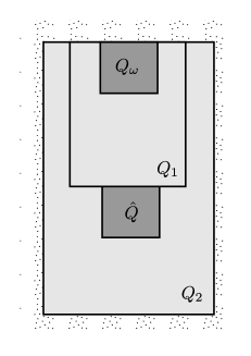
Figure 1. Cylinders involved in the statement of the De Giorgi intermediate-value Lemma.

Lemma 14 (A De Giorgi intermediate-value lemma).

Let $\omega=\frac{1}{4}$. For any (universal) constants $\delta_{1}\in(0,1)$, $\delta_{2}\in(0,1)$ there exist $\nu>0$ and $\theta\in(0,1)$ (both universal) such that for any sub-solution $f$ of (1.6) in $Q_{2}$ with

$$f\leq 1\quad\text{ and }\quad|s|\leq 1$$

and

$$|\{f\geq 1-\theta\}\cap Q_{\omega}| \geq\delta_{1}|Q_{\omega}|$$

$$|\{f\leq 0\}\cap\hat{Q}| \geq\delta_{2}|\hat{Q}|$$

we have

$$|\{0<f<1-\theta\}\cap B_{1}\times B_{1}\times(-2,0]|\geq\nu.$$

Remark 15.

While De Giorgi’s isoperimetric inequality is based on an explicit computation leading to a precise estimate with effective constants, the proof of Lemma 14 is obtained by an argument by contradiction, so that the values of $\theta$ and $\nu$ are not known explicitly.

Remark 16.

The compactness argument used in the proof is reminiscent of one used by Guo in [41] and of one used by the fourth author in [58].

Proof.

We argue by contradiction by assuming that there exists a sequence $(f_{k})_{k\geq 0}$ of sub-solutions:

(4.1) $$(\partial_{t}+v\cdot\nabla_{x})f_{k}\leq\nabla_{v}\cdot(A_{k}\nabla_{v}f_{k})+B_{k}\cdot\nabla_{v}f_{k}+s_{k}$$

such that $f_{k}\leq 1$ and $|s_{k}|\leq 1$ and

$$\begin{cases}\theta_{k}\to 0\\[2.84526pt] \alpha_{k}\to 0\end{cases}\quad\text{ as }\quad k\to+\infty$$

and

$$|\{f_{k}\geq 1-\theta_{k}\}\cap Q_{\omega}| \geq\delta_{1}|Q_{\omega}|$$

$$|\{f_{k}\leq 0\}\cap\hat{Q}| \geq\delta_{2}|\hat{Q}|$$

$$|\{0<f_{k}<1-\theta_{k}\}\cap(Q_{1}\cup\hat{Q})| \to 0\quad\text{ as }\quad k\to+\infty.$$

The convexity of $z\mapsto z^{+}$ together with $|s_{k}|\leq 1$ implies that the non-negative part $f_{k}^{+}$ of $f_{k}$ satisfies the same inequation, and therefore

(4.2) $$(\partial_{t}+v\cdot\nabla_{x})f_{k}^{+}=\nabla_{v}\cdot(A_{k}\nabla_{v}f_{k}^{+})+B_{k}\cdot\nabla_{v}f_{k}^{+}+1-\mu_{k}$$

for some non-negative measures $\mu_{k}$.

A priori estimates for $f_{k}^{+}$. The natural energy estimate is obtained by multiplying the equation with $f_{k}^{+}\Psi^{2}$ with a smooth cut-off function $\Psi$ supported in $Q_{2}$ and valued in $[0,1]$, and using the fact that $f_{k}^{+}\leq 1$ and $|s_{k}|\leq 1$:

$$\lambda\int_{{\mathbb{R}}^{2d+1}}|\nabla_{v}f_{k}^{+}|^{2}\Psi^{2} \leq\bar{C}\int_{{\mathbb{R}}^{2d+1}}\left(\Psi^{2}+|\nabla_{v}\Psi|^{2}+\Psi|(\partial_{t}+v\cdot\nabla_{x})\Psi|\right)+\Lambda\int_{{\mathbb{R}}^{2d+1}}|\nabla_{v}f_{k}^{+}|f_{k}^{+}\Psi^{2}$$

$$\leq\bar{C}\int_{{\mathbb{R}}^{2d+1}}\left(\Psi^{2}+|\nabla_{v}\Psi|^{2}+\Psi|(\partial_{t}+v\cdot\nabla_{x})\Psi|\right)+\frac{\lambda}{2}\int_{{\mathbb{R}}^{2d+1}}|\nabla_{v}f_{k}^{+}|^{2}\Psi^{2}.$$

Hence

(4.3) $$\lambda\int_{{\mathbb{R}}^{2d+1}}|\nabla_{v}f_{k}^{+}|^{2}\Psi^{2}\leq\bar{C}\int_{{\mathbb{R}}^{2d+1}}\left(\Psi^{2}+|\nabla_{v}\Psi|^{2}+\Psi|(\partial_{t}+v\cdot\nabla_{x})\Psi|\right)$$

where $\bar{C}=\bar{C}(d,\lambda,\Lambda)$.

We can also multiply the equation by $\Psi^{2}$ and get

$$-\int_{{\mathbb{R}}^{2d+1}}f_{k}^{+}(\partial_{t}+v\cdot\nabla_{x})(\Psi^{2})=-\int_{{\mathbb{R}}^{2d+1}}A_{k}\nabla_{v}f_{k}^{+}\cdot\nabla_{v}(\Psi^{2})+\int_{{\mathbb{R}}^{2d+1}}B_{k}\cdot\nabla_{v}f_{k}^{+}\Psi^{2}\\ +\int_{{\mathbb{R}}^{2d+1}}\Psi^{2}-\int_{{\mathbb{R}}^{2d+1}}\Psi^{2}{\,\mathrm{d}}\mu_{k}.$$

Combining the latter equation with (4.3), we deduce

(4.4) $$\int_{{\mathbb{R}}^{2d+1}}\Psi^{2}{\,\mathrm{d}}\mu_{k}\leq\bar{C}\int_{{\mathbb{R}}^{2d+1}}\left(\Psi^{2}+|\nabla_{v}\Psi|^{2}+\Psi|(\partial_{t}+v\cdot\nabla_{x})\Psi|\right)$$

where $\bar{C}=\bar{C}(d,\lambda,\Lambda)$.

Passage to the limit. On the one hand, Banach-Alaoglu theorem implies that

$$f_{k}^{+}\stackrel{{\scriptstyle\ast}}{{\rightharpoonup}}F\text{ in }L^{\infty}_{\text{loc}}(Q_{2})$$

and

(4.5) $$\nabla_{v}f_{k}^{+}\rightharpoonup\nabla_{v}F\quad\text{ and }\quad\begin{cases}A_{k}\nabla_{v}f_{k}^{+}\rightharpoonup H_{1}\\[5.69054pt] B_{k}\cdot\nabla_{v}f_{k}^{+}\rightharpoonup H_{0}\end{cases}\text{ in }L^{2}_{\text{loc}}(Q_{2})$$

for some weak limit $F\in L^{\infty}_{\text{loc}}(Q_{2})\cap(L^{2}_{x,t}H^{1}_{v})_{\text{loc}}(Q_{2})$. In particular, (4.3) implies that

(4.6) $$\int_{Q}|\nabla_{v}F|^{2}\lesssim_{Q}1$$

for all $Q\Subset Q_{2}$, with a control depending on $Q$. On the other hand, the bound (4.4) implies that

$$\mu_{k}\rightharpoonup\mu\quad\text{ in }\mathcal{M}(Q_{2}).$$

We thus have

(4.7) $$(\partial_{t}+v\cdot\nabla_{x})F=\nabla_{v}H_{1}+H_{0}+1-\mu.$$

By velocity averaging (see Theorem 1.8 in [8]), together with the bound (4.3), we deduce the strong convergence

$$f_{k}^{+}\to F\text{ in }L^{p}_{\text{loc}}(Q_{2})\quad\text{ for }1\leq p<+\infty.$$

It implies the convergence in probability and thus the function $F$ satisfies

(4.8) $$|\{F=1\}\cap Q_{\omega}| \geq\delta_{1}|Q_{\omega}|$$

(4.9) $$|\{F=0\}\cap\hat{Q}| \geq\delta_{2}|\hat{Q}|$$

$$\left|\{0<F<1\}\cap\left(B_{1}\times B_{1}\times(-2,0]\right)\right| =0\,.$$

In view of (4.6), since indicator functions are not in $H^{1}$ unless they are constant, we have that for almost every $(x,t)\in B_{1}\times(-1,0)$,

$$\left\{\begin{aligned} \text{either }\quad&\mbox{for almost every }v\in B_{1},\quad F(x,v,t)=0\\[2.84526pt] \text{ or }\quad\quad&\mbox{for almost every }v\in B_{1},\quad F(x,v,t)=1.\end{aligned}\right.$$

In other words, $F(x,v,t)=\mathbf{1}_{P}(x,t)$ for some measurable set $P\subset B_{1}\times(-1,0)$. In view of (4.8) and (4.9), $P$ satisfies

(4.10) $$\begin{cases}|P\cap B_{\omega^{3}}\times(-\omega^{2},0)|>0\\[5.69054pt] |B_{\omega^{3}}\times(-1-\omega^{2},-1)\setminus P|>0.\end{cases}$$

Propagation. We thus get from (4.7)

$$\partial_{t}F+v\cdot\nabla_{x}F\leq\nabla_{v}H_{1}+H_{0}+1\quad\text{ in }B_{1}\times B_{1}\times(-2,0).$$

Consider a cut-off funtion $\xi\in\mathcal{D}({\mathbb{R}}^{d})$ such that

$$\int_{{\mathbb{R}}^{d}}\zeta(z){\,\mathrm{d}}z=1,\quad\zeta(z)=\zeta(-z),\quad\operatorname{supp}\zeta\subset B_{\frac{1}{2}}.$$

Given $v_{0}\in B_{\frac{1}{2}}$, since $F$ only depends on $(t,x)$, we can use a test-function of the form $\zeta(v-v_{0})$, and get for all $v_{0}\in B_{\frac{1}{2}}$,

$$\partial_{t}F+v_{0}\cdot\nabla_{x}F\leq\int_{{\mathbb{R}}^{d}}\Big{[}\left|H_{1}(x,v,t)\nabla_{v}\zeta(v-v_{0})\right|+\left|H_{0}(x,v,t)\zeta(v-v_{0})\right|\Big{]}{\,\mathrm{d}}v+1$$

in $(x,t)\in B_{1}\times(-2,0)$. Since $F$ is an indicator function and $H_{0},H_{1}\in L^{2}_{\text{loc}}(Q_{2})$, this implies for $v_{0}\in B_{\frac{1}{2}}$,

(4.11) $$\partial_{t}F+v_{0}\cdot\nabla_{x}F\leq 0\quad\text{ in }B_{1}\times(-2,0).$$

We next remark that

(4.12) $$\begin{cases}\text{ for all }(x,t)\in B_{\omega^{3}}\times(-\omega^{2},0)\quad\text{ and }\quad(x_{0},t_{0})\in B_{\omega^{3}}\times(-1-\omega^{2},-1),\\[5.69054pt] \text{ there exists }v_{0}\in B_{\omega}\mbox{ so that }(x_{0},v_{0},t_{0})\in\hat{Q}\text{ and }(x,t)=(x_{0}+sv_{0},t_{0}+s).\end{cases}$$

Indeed, the time shift $s$ is fixed by $t=t_{0}+s$ and belongs to $(1-\omega^{2},1+\omega^{2})$. Then the velocity $v_{0}$ is fixed by $x=x_{0}+sv_{0}$ and satisfies

$$|v_{0}|=\frac{|x-x_{0}|}{t-t_{0}}<\frac{2\omega^{3}}{1-\omega^{2}}\leq\omega$$

since $\omega=\frac{1}{4}\leq\frac{1}{\sqrt{3}}$. Since $|B_{1}\times(-1-\omega^{2},-1)\setminus P|>0$ (see (4.10)), we can use (4.11) and (4.12) and conclude that $F\equiv 0$ in $Q_{\omega}$, and contradicts (4.10). The proof is complete. ∎

4.2. Improvement of oscillation

It is classical that Hölder continuity is a consequence of the decrease of the oscillation of the solution “at unit scale”.

Lemma 17 (Improvement of oscillation).

There exist $\lambda_{0}\in(0,1)$, $\omega\in(0,1/2)$ and $\beta>0$ (all universal) such that any $f$ solution of (1.6) in $Q_{2}$ with $\operatorname{osc}_{Q_{2}}f\leq 2$ and $|s|\leq\beta$ satisfies

$$\operatorname{osc}_{Q_{\frac{\omega}{2}}}f\leq 2-\lambda_{0}.$$

This lemma is a consequence of the following one.

Lemma 18 (A measure-to-pointwise estimate).

Given $\delta_{2}>0$, there exist $\lambda_{0}\in(0,1)$, $\omega\in(0,1/2)$ and $\beta>0$ (depending on $\delta_{2}$ but not on the sub-solution) such that any $f$ sub-solution of (1.6) in $Q_{2}$ with $f\leq 1$ and $|s|\leq\beta$ such that $|\{f\leq 0\}\cap\hat{Q}|\geq\delta_{2}|\hat{Q}|$ satisfies

(4.13) $$f\leq 1-\lambda_{0}\quad\text{a.e. in }\quad Q_{\frac{\omega}{2}}.$$

Proof of Lemma 17.

Let $f$ be a solution of (1.6) in $Q_{2}$ with $\operatorname{osc}_{Q_{2}}f\leq 2$ and $|s|\leq\beta$. We can reduce to the case where $|f|\leq 1$. Indeed, we remark that there exists a constant $C$ such that $\tilde{f}=f-C$ satisfies (1.6) in $Q_{2}(0)$ with $|\tilde{f}|\leq 1$ and the same source term.

If $|\{f\leq 0\}\cap\hat{Q}|\geq|\hat{Q}|/2$, then apply Lemma 18 with $\delta_{2}=1/2$.

In the other case, considering $-f$ implies that the essential infimum of $f$ is raised. In both cases, we get the desired improvement of the oscillation of $f$. This completes the proof of the lemma. ∎

We now turn to the proof of Lemma 18.

Proof of Lemma 18.

The proof proceeds in several steps.

Choice of parameters. Theorem 12 provides us with $\kappa$ correponding to the upper bound $\mathfrak{g}=1$ on the source term and $Q_{\mathrm{ext}}=Q_{\omega}$ and $Q_{\infty}=Q_{\frac{\omega}{2}}$. Lemma 14 applied with $\delta_{2}$ and $\delta_{1}=\sqrt{\kappa}/|Q_{\omega}|$ provides us with $\nu$ and $\theta$ universal. We choose next $k_{0}$ the smallest positive integer such that

$$k_{0}\nu>|B_{1}\times B_{1}\times(-2,0)|.$$

We finally choose $\beta$ such that $\beta\leq\theta^{k_{0}}$.

Iteration. We define $f_{0}=f$ and

$$f_{k+1}=\frac{1}{\theta}(f_{k}-(1-\theta))=\theta^{-k}(f-(1-\theta^{k})).$$

They satisfy $f_{k}\leq 1$ and

$$(\partial_{t}+v\cdot\nabla_{x})f_{k}\leq\nabla_{v}\cdot(A\nabla_{v}f_{k})+B\cdot\nabla_{v}f_{k}+s_{k}$$

with $s_{k}=\theta^{-k}s$. In particular $|s_{k}|\leq\theta^{-k_{0}}\beta\leq 1$ which allows to apply Theorem 12 with the upper bound $\mathfrak{g}=1$ as above. Remark that

(4.14) $$|\{f_{0}\leq 0\}\cap\hat{Q}|\geq\delta_{2}|\hat{Q}|\quad\mbox{ and }\quad\{f_{k+1}\leq 0\}\supset\{f_{k}\leq 0\}.$$

Our goal is to prove that there exists at least one index $k\in\{1,\dots,k_{0}\}$ such that

$$|\{f_{k}\geq 0\}\cap Q_{\omega}|\leq\delta_{1}|Q_{\omega}|.$$

Indeed, remarking that for such an index $k_{1}$

$$\|(f_{k_{1}})_{+}\|_{L^{2}(Q_{\omega})}\leq\bigg{[}\big{|}\{f_{k_{1}}\geq 0\}\cap Q_{\omega}\big{|}\bigg{]}^{\frac{1}{2}}\leq\sqrt{\delta_{1}|Q_{\omega}|}\leq\kappa,$$

Theorem 12 then implies that

$$f\leq 1-\frac{1}{2}\theta^{k_{1}}\leq 1-\frac{1}{2}\theta^{k_{0}}\quad\text{ in }\quad Q_{\frac{\omega}{2}}$$

which concludes the proof.

Let us prove the claim by contradiction. Assume that for all $k=1,\dots,k_{0}$,

$$|\{f_{k}\geq 0\}\cap Q_{\omega}|\geq\delta_{1}|Q_{\omega}|.$$

Since $f_{k+1}=\frac{1}{\theta}(f_{k}-(1-\theta))$, this also implies for $k=0,\dots,k_{0}-1$,

$$|\{f_{k}\geq 1-\theta\}\cap Q_{\omega}|\geq\delta_{1}|Q_{\omega}|.$$

But (4.14) also implies that for all $k\geq 0$,

$$|\{f_{k}\leq 0\}\cap\hat{Q}|\geq\delta_{2}|\hat{Q}|.$$

Hence Lemma 14 implies that for $k=0,\dots,k_{0}-1$,

$$\left|\{0\leq f_{k}\leq 1-\theta\}\cap\left(B_{1}\times B_{1}\times(-2,0)\right)\right|\geq\nu.$$

Now remark that

$$\left|\{f_{k+1}\leq 0\}\cap\left(B_{1}\times B_{1}\times(-2,0)\right)\right|= \left|\{f_{k}\leq 0\}\cap\left(B_{1}\times B_{1}\times(-2,0)\right)\right|$$

$$+\left|\{0\leq f_{k}\leq 1-\theta\}\cap\left(B_{1}\times B_{1}\times(-2,0)\right)\right|$$

$$\geq \left|\{f_{k}\leq 0\}\cap\left(B_{1}\times B_{1}\times(-2,0)\right)\right|+\nu.$$

In particular

$$\left|B_{1}\times B_{1}\times(-2,0)\right|\geq\left|\{f_{k_{0}}\leq 0\}\cap\left(B_{1}\times B_{1}\times(-2,0)\right)\right|\geq k_{0}\nu$$

which is impossible for $k_{0}$ as chosen above. The proof is now complete. ∎

4.3. Proof of the Hölder estimate

Proof of Theorem 3.

Consider an $L^{2}$ solution $f$ of Eq. (1.6) in a cylinder $Q_{\mathrm{ext}}=Q_{r_{0}}(z_{0})$. By Theorem 12, we know that $f$ is locally bounded in $Q_{\mathrm{ext}}$. In particular, $f$ is bounded in $Q_{\mathrm{mid}}=Q_{\frac{r_{0}+r_{1}}{2}}(z_{0})$ and

$$\|f\|_{L^{\infty}(Q_{\mathrm{mid}})}\leq C_{0}\left(\|f\|_{L^{2}(Q_{\mathrm{ext}})}+\|s\|_{L^{\infty}(Q_{\mathrm{ext}})}\right)$$

for some constant $C_{0}=C(d,\lambda,\Lambda,Q_{\mathrm{ext}},Q_{\mathrm{mid}})$. If $f\equiv 0$ in $Q_{\mathrm{ext}}$, there is nothing to prove. If $f$ is not identically $0$, recalling that $\beta$ is given by Lemma 17, we assume that

$$\|f\|_{L^{\infty}(Q_{\mathrm{mid}})}\leq 1\quad\text{ and }\quad\|s\|_{L^{\infty}(Q_{\mathrm{ext}})}\leq\beta$$

by considering, if necessary,

$$\tilde{f}=\frac{f}{C_{0}\left(\|f\|_{L^{2}(Q_{\mathrm{ext}})}+\|s\|_{L^{\infty}(Q_{\mathrm{ext}})}\right)+\beta^{-1}\|s\|_{L^{\infty}(Q_{\mathrm{ext}})}}.$$

Let $z_{1}\in Q_{\mathrm{int}}:=Q_{r_{1}}(z_{0})$. We want to prove that for all $r>0$ such that $Q_{2r}(z_{1})\subset Q_{\mathrm{mid}}$,

(4.15) $$\operatorname{osc}_{Q_{r}(z_{1})}f\leq Cr^{\alpha}$$

for some universal $\alpha\in(0,1)$ and some constant $C=C(d,\lambda,\Lambda,r_{0},r_{1})$. Let $\tilde{r}>0$ denote the largest $r\in(0,1)$ such that $Q_{2r}(z_{0})\subset Q_{\mathrm{mid}}$. We remark that for $r\in(0,\tilde{r})$, $Q_{2r}(z_{1})=\mathcal{T}^{-1}_{z_{1}}(Q_{2r})$ where $\mathcal{T}_{z_{1}}$ is defined in Eq. (1.8) and $\bar{f}=f\circ\mathcal{T}_{z_{1}}$ satisfies (1.6) in $Q_{2\tilde{r}}$ with the source term $\bar{s}:=s\circ\mathcal{T}_{z_{1}}$ and the coefficients $\bar{A}:=A\circ\mathcal{T}_{z_{1}}$ and $\bar{B}:=B\circ\mathcal{T}_{z_{1}}$. In particular $\bar{f}$ and $\bar{s}$ satisfy

$$\|\bar{f}\|_{L^{\infty}(Q_{2\tilde{r}})}\leq 1\quad\text{ and }\quad\|\bar{s}\|_{L^{\infty}(Q_{2\tilde{r}})}\leq\beta$$

and (4.15) is equivalent to: for all $r\in(0,\tilde{r})$,

(4.16) $$\operatorname{osc}_{Q_{r}}\bar{f}\leq Cr^{\alpha}.$$

We recall how to scale solutions. For all $r\in(0,\tilde{r})$, the function

$$\bar{f}_{r}(x,v,t)=\bar{f}(r^{3}x,rv,r^{2}t)$$

is defined in $Q_{2}$ and satisfies (1.6) with

$$\begin{cases}\bar{B}_{r}(x,v,t)=r\bar{B}(r^{3}x,rv,r^{2}t)\\[5.69054pt] \bar{s}_{r}(x,v,t)=r^{2}\bar{s}(r^{3}x,rv,r^{2}t).\end{cases}$$

Since $\operatorname{osc}_{Q_{2\tilde{r}}}\bar{f}\leq 2$, we have $\operatorname{osc}_{Q_{2}}\bar{f}_{\tilde{r}}\leq 2$ and Lemma 17 implies that

$$\operatorname{osc}_{Q_{\frac{\omega}{2}}}\bar{f}_{\tilde{r}}=\operatorname{osc}_{Q_{\frac{\omega}{2}\tilde{r}}}\bar{f}\leq 2\theta$$

with $\theta=1-\lambda_{0}/2$ (we used the fact that $\tilde{r}\leq 1$ to ensure that $\|\bar{s}_{\tilde{r}}\|_{L^{\infty}(Q_{2})}\leq\beta$). We remark that we can assume that $\theta\geq 1/2$ and we recall that $\omega\in(0,1/2)$. We next apply Lemma 17 to $\theta^{-1}\bar{f}_{\tilde{r}_{1}}$ with $\tilde{r}_{1}=(\omega/4)\tilde{r}$, which rescales the $L^{\infty}$ bound on the source term by a factor $(\omega/4)^{2}\theta^{-1}<1$ as compared to $\|\bar{s}_{\tilde{r}}\|_{L^{\infty}(Q_{2})}\leq\beta$. Hence the bounds assumed are still valid and we get

$$\operatorname{osc}_{Q_{\tilde{r}_{2}}}\bar{f}\leq 2\theta^{2}$$

with $\tilde{r}_{2}=(\omega/2)\tilde{r}_{1}$. Inductively, we deduce that

$$\operatorname{osc}_{Q_{\tilde{r}_{k}}}\bar{f}\leq 2\theta^{k}$$

with $\tilde{r}_{k}=(\omega/2)^{k}\tilde{r}/2$. This yields (4.16) for $r=\tilde{r}_{k}$ with

$$\alpha=\frac{\ln\theta}{\ln(\omega/2)}\quad\text{ and }\quad C=2\left(\frac{2}{\tilde{r}}\right)^{\alpha}.$$

If now $r\in[\tilde{r}_{k+1},\tilde{r}_{k}]$, then

$$\operatorname{osc}_{Q_{r}}\bar{f}\leq\operatorname{osc}_{Q_{r_{k}}}\bar{f}\leq C\tilde{r}_{k}^{\alpha}=C\left(\frac{2}{\omega}\right)^{\alpha}\tilde{r}_{k+1}^{\alpha}\leq\tilde{C}r^{\alpha}$$

with $\tilde{C}=C(2/\omega)^{\alpha}$. Observe finally that the constant $C$ and $\tilde{C}$ are uniformly bounded above as $z_{0}$ varies in $Q_{\mathrm{int}}$ since $\tilde{r}\geq r_{1}-r_{0}$. The proof is now complete. ∎

5. Harnack inequality

In this section, we derive Harnack inequality for solutions to Eq. (1.6). We use here an approach that Luis Silvestre explained to us in the stationary setting: we start with Hölder continuous solutions and we consider expanding cylinders to control the spreading of the lower bound of non-negative solutions (see Lemma 23). The Harnack inequality is a consequence of the decrease of oscillation we proved earlier and a so-called “doubling property” that estimates how the minimum of a solution propagates with time. Let us first recall the decrease of oscillation proposition.

Proposition 19 (Decrease of oscillation).

There exist $\delta\in(0,1)$ and $\omega\in(0,1/2)$ (both universal) such that for any $r\in(0,1)$ and any solution $f$ of (1.6) in some cylinder $Q_{2r}(z)$ satisfies

$$\operatorname{osc}_{Q_{\frac{\omega}{4}r}(z)}f\leq(1-\delta)\left(\operatorname{osc}_{Q_{r}(z)}f+2\beta^{-1}\|s\|_{L^{\infty}}\right).$$

Remark 20.

The conclusion of the proposition is equivalent to

$$\operatorname{osc}_{Q_{\frac{\omega}{4}r}}f\circ\mathcal{T}_{z}\leq(1-\delta)\left(\operatorname{osc}_{Q_{r}}f\circ\mathcal{T}_{z}+2\beta^{-1}\|s\|_{L^{\infty}}\right)$$

with $\mathcal{T}_{z}(y,w,s)=(x+y+sv,v+w,t+s)$ where $z=(x,v,t)$.

Proof.

By considering

$$\tilde{f}=\frac{f\circ\mathcal{T}_{z}}{\operatorname{osc}_{Q_{2r}(z)}f/2+\|s\|_{L^{\infty}}/\beta},$$

and a rescaling $\tilde{f}_{r}$, we can assume that $z=0$ and $\operatorname{osc}_{Q_{2}}\tilde{f}_{r}\leq 2$ and $\|s\|_{L^{\infty}}\leq\beta$ (we use here that $r\leq 1$). We then apply Lemma 17 to $\tilde{f}_{r}$ and get the desired result with $1-\delta=1-\lambda_{0}/2$. ∎

5.1. How minima propagate with time

The goal of this subsection is to prove the following proposition. In order to state it, we introduce two cylinders which contain $Q^{-}$:

$$Q^{-}\subset Q^{-}[1]\subset Q^{-}[2]\subset Q_{1}.$$

See Figure 2.

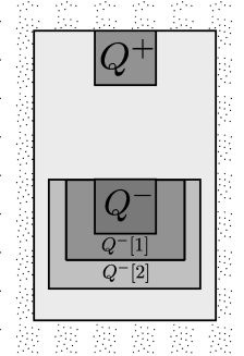
Figure 2. The cylinders $Q^{+}$, $Q^{-}$, $Q^{-}[1]$ and $Q^{-}[2]$. Harnack inequality relates the supremum of a solution over $Q^{-}$ and its infimum over $Q^{+}$. The proof consists in constructing a sequence of points lying in $Q^{-}[1]$ and whose corresponding values explode. Neighborhoods of points included in $Q^{-}[2]$ are also considered.

We recall that $Q^{+}=Q_{R}$ and $Q^{-}=Q_{R}(0,0,-\Delta)$ and $R,\Delta\in(0,1)$ are small so that in particular $Q^{\pm}\subset Q_{1}$ and they are disjoint. We let $Q^{-}[i]$ be equal to $Q_{\rho_{i}}(0,0,-\Delta)$ with $R<\rho_{1}<\rho_{2}<1$.

In the following propositions, we introduce elongated cylinders $Q^{\mathit{el}}$ where the time is stretched longer in the past than what the scaling would induce:

$$Q^{\mathit{el}}_{1} =B_{(\omega/4)^{3}}\times B_{\omega/4}\times(-1,0]$$

$$Q^{\mathit{el}}_{r}(z) =\mathcal{T}_{z}\big{(}B_{(\omega/4)^{3}r^{3}}\times B_{(\omega/4)r}\times(-r^{2},0]\big{)}.$$

Proposition 21 (The propagation of minima).

Assume that $f$ is a non-negative super-solution of (1.6) in $Q_{1}$ with a non-negative source term $s$. There exists $r_{0}>0$, $R>0$ (universal) such that for any $r\in(0,r_{0})$ and $z\in Q^{-}$ such that $Q^{\mathit{el}}_{r}(z)\subset Q^{-}[2]$, we have

$$\min_{Q^{\mathit{el}}_{r}(z)}f\leq C_{\text{{\em pm}}}\;r^{-q}\min_{Q^{+}}f$$

for some universal constants $C_{\text{{\em pm}}}$ and $q>0$.

We first derive from Lemma 18 the following doubling property at the origin. For the two next lemmas, it is easier that $0$ is the final time of the first cylinder.

Lemma 22 (The doubling property at the origin).

There exists $\mathfrak{h}\in(0,1)$ (universal) such that for any non-negative super-solution $f$ of (1.6) in $B_{8}\times B_{2}\times(-1,4]$ with $s\geq 0$, we have

$$\inf_{Q^{1}}f\geq\mathfrak{h}\inf_{Q^{0}}f$$

with $Q^{1}=Q^{\mathit{el}}_{2}(0,0,4)$ and $Q^{0}=Q^{\mathit{el}}_{1}$.

Proof.

We first note that since $s\geq 0$, the function $f$ is a super-solution of (1.6) with $s=0$. We first prove that

(5.1) $$\inf_{Q_{\omega/2}(0,0,1)}f\geq\mathfrak{h}_{0}\inf_{Q_{\omega/4}}f$$

for some universal constant $\mathfrak{h}_{0}$; see Figure 3.

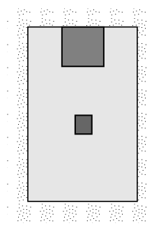
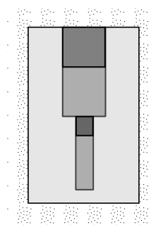
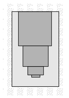
Figure 3. The doubling property. On the left, the cylinders $Q_{\omega/4}$ and $Q_{\omega/2}(0,0,1)$. In the middle, the elongated cylinders $Q^{0}$ and $Q^{1}$. On the right, the iterated cylinders $Q^{0},\dots,Q^{N}$ (Lemma 23).

If $\inf_{Q_{\omega/4}}f=0,$ there is nothing to prove. If not, the function

$$g=\frac{f}{\inf_{Q_{\omega/4}}f}$$

satisfies (1.6) in $Q_{2}$ (up to translation in time – this is where we use that $s=0$) and

$$|\{g\geq 1\}\cap Q_{\omega}|\geq|Q_{\omega/4}|=\delta_{2}|Q_{\omega}|$$

for some universal $\delta_{2}$, where $Q_{\omega}$ plays the role of $\hat{Q}$ in Lemma 18. We then apply Lemma 18 (with time shifted by $+1$) to $\tilde{g}=1-g\leq 1$, we get $g\geq\mathfrak{h}_{0}$ in $B_{(\omega/2)^{3}}\times B_{\omega/2}\times(1-(\omega/2)^{2},1]$, that is to say, (5.1) indeed holds true.

Apply now the result to $\tilde{f}(x,v,t)=f(x,v,t-T)$ for $T\in[0,1-\omega^{2}]$ and get

(5.2) $$\inf_{B_{(\omega/2)^{3}}\times B_{\omega/2}\times(0,1]}f\geq\mathfrak{h}_{0}\inf_{Q^{0}}f.$$

By applying (5.2) on time intervals $(1,2]$, $(2,3]$ and $(3,4]$, we propagate the infimum till time $t=4$ and get the desired result for $\mathfrak{h}=\mathfrak{h}_{0}^{4}$. ∎

Applying iteratively the previous lemma, we obtain straightforwardly the following lemma whose proof is omitted.

Lemma 23 (The iterated doubling property at the origin).

There exists $\mathfrak{h}>0$ (universal) such that for any $f$ non-negative super-solution of (1.6) in $B_{2^{3N}}\times B_{2^{N}}\times(-1,T^{N})$, we have

(5.3) $$\inf_{Q^{N}}f\geq\mathfrak{h}^{N}\inf_{Q^{0}}f$$

with

$$Q^{k}=B_{R_{k}^{3}}\times B_{R_{k}}\times(T_{k-1},T_{k}]\quad\text{ for }\quad k\geq 1$$

where $R_{k}=(\omega/4)2^{k}$ and $T_{k}=\frac{4}{3}(4^{k}-1)$ for $k\geq 0$.

Remark 24.

In [44], a measure estimate is also applied iteratively to prove a Harnack inequality for fully nonlinear parabolic equations in non-divergence form.

We can now prove Proposition 21.

Proof of Proposition 21.

In the following proof, we need iterated cylinders that are not centered at the origin and with arbitrary radius.

$$Q^{k}_{r}(z):=\mathcal{T}_{z}\big{(}rQ^{k}\big{)}.$$

The cylinder $Q^{k}$ is first scaled by $r$ (this is $rQ^{k}$) and then centered around $z$ (this is $\mathcal{T}_{z}\big{(}rQ^{k}\big{)}$).

Let $z_{\infty}\in Q^{+}$ be such that $\min_{Q^{+}}f=f(z_{\infty})$.

Lemma 25.

There exist $R$, $\Delta$, $r_{0}$ (small, universal) such that

1. for all $r\in(0,r_{0})$ and $z\in Q^{-}$, the iterated cylinders $Q^{k}_{r}(z)$ ($k\in{\mathbb{N}}$) which are included in $\{t\leq 0\}$ are in fact included in $Q_{1}(0)$;

2. the union of the iterated cylinders $\bigcup_{k=1}^{+\infty}Q^{k}_{r}(z)$ contains $Q^{+}$.

The proof is elementary but tedious. It is given in Appendix.

Applying Lemma 23, we get

$$\inf_{Q^{\mathit{el}}_{r}(z)}f\leq\mathfrak{h}^{-N}\inf_{Q^{N}_{r}(z)}f\leq\mathfrak{h}^{-N}\min_{Q^{+}}f$$

with $N$ such that $z_{\infty}\in Q^{N}_{r}(z)$, i.e. $r^{-1}(z^{-1}\circ z_{\infty})\in Q^{N}$. In particular, $r^{-2}(t_{\infty}-t)\in[T^{N-1},T^{N}]$. Since $z_{\infty}\in Q^{+}$ and $z\in Q^{-}$, we know that

$$4^{N-1}\leq T^{N-1}\leq\frac{t_{\infty}-t}{r^{2}}\leq\frac{1/2+R^{2}}{r^{2}}.$$

In particular,

$$\mathfrak{h}^{-N}\leq\left(\frac{1/2+R^{2}}{4}\right)^{\frac{q}{2}}r^{-q}$$

where $q=-\ln\gamma/\ln 2>0$. We get the desired inequality with $C_{\text{pm}}=((1/2+R^{2})/4)^{\frac{q}{2}}$. The proof of the proposition is thus complete. ∎

5.2. Proof of the Harnack inequality

We can now turn to the proof of Theorem 4.

Proof of Theorem 4.

We first remark that replacing $f(x,v,t)$ with $f(x,v,t)+\|s\|_{L^{\infty}}t$ if necessary, we can assume that $s\geq 0$. Dividing $f$ by $2\beta^{-1}\|s\|_{L^{\infty}}$ if necessary, we can assume that $\|s\|_{L^{\infty}}=\beta/2$ (if $s\not\equiv 0$).

We are going to find a universal constant $C=C_{H}$ such that (1.10) cannot hold false. In other words, we are going to find a universal $C_{H}$ such that

(5.4) $$m+1\leq C_{H}M$$

entails a contradiction where

$$M:=\sup_{Q^{-}}f=f(z_{0})\quad\text{ and }\quad m:=\inf_{Q^{+}}f=f(z_{\infty})$$

for some $z_{0}\in Q^{-}$ and $z_{\infty}\in Q^{+}$. We used here the fact that $u$ is (Hölder) continuous.

Our goal is to construct by induction a sequence $(z_{k})_{k\geq 0}$ in $Q^{-}[1]$ (we recall that $Q^{-}\subset Q^{-}[1]\subset Q^{-}[2]\subset Q_{1}$, see Figure 2) such that

(5.5) $$f(z_{k})\geq(1-\delta^{\prime})^{-k}M$$

for some universal $\delta^{\prime}\in(0,1)$. This implies in particular that $f(z_{k})\to+\infty$ as $k\to+\infty$ which is absurd since $f$ is bounded in $Q^{-}$.

Remark first that (5.5) holds true for $k=0$. Let us assume that we already constructed $z_{0},\dots,z_{k}$ and let us construct $z_{k+1}$. Let $z_{k}=(x_{k},v_{k},t_{k})$. We choose $r_{k}>0$ such that

(5.6) $$f(z_{k})=r_{k}^{-2q}m$$

where $q$ is given by Proposition 21. Inequality (5.4) and the induction hypothesis (5.5) imply

(5.7) $$r_{k}^{2q}\leq C_{H}(1-\delta^{\prime})^{k}.$$

From the decrease of oscillation (Proposition 19), we know that

$$1+\operatorname{osc}_{Q_{r_{k}}}f\geq(1-\delta)^{-1}\operatorname{osc}_{q_{k}}f$$

(recall $2\beta^{-1}\|s\|_{L^{\infty}}=1$) with

$$Q_{k}=Q_{r_{k}}(z_{k})\quad\text{ and }\quad q_{k}=Q_{\omega r_{k}/4}(z_{k}).$$

In particular, $z_{k}\in q_{k}$. Let $z_{k+1}\in Q_{k}$ be such that

$$\max_{Q_{k}}f=f(z_{k+1}).$$

Then we get

(5.8) $$1+f(z_{k+1})\geq(1-\delta)^{-1}\left(f(z_{k})-\min_{q_{k}}f\right).$$

Recall that $z_{k}\in Q^{-}[1]$. Choosing $C_{H}$ small, we can ensure through (5.7) that $Q_{r_{k}}(z_{k})\subset Q^{-}[2]$. We also remark that

$$q_{k}\supset Q^{\mathit{el}}_{(\omega/4)^{2}r_{k}}(z_{k}).$$

We thus can apply Proposition 21 and get

$$\min_{q_{k}}f\leq\min_{Q^{\mathit{el}}_{(\omega/4)^{2}r_{k}}(z_{k})}f\leq\tilde{C}_{\text{pm}}r_{k}^{-q}m$$

with $\tilde{C}_{\text{pm}}=C_{\text{pm}}(4/\omega)^{q}$. The use of (5.6) in the previous inequality yields

(5.9) $$\min_{q_{k}}f\leq\tilde{C}_{\text{pm}}r_{k}^{q}f(z_{k})\leq\tilde{C}_{\text{pm}}\sqrt{C_{H}}f(z_{k}).$$

Now combining (5.8) and (5.9), we get

$$1+f(z_{k+1})\geq(1-\delta)^{-1}(1-\tilde{C}_{\text{pm}}\sqrt{C_{H}})f(z_{k}).$$

Use next that $1\leq C_{H}M$ (this is a consequence of (5.4)) and the induction hypothesis and get

$$f(z_{k+1}) \geq(1-\delta)^{-1}(1-\tilde{C}_{\text{pm}}\sqrt{C_{H}})(1-\delta^{\prime})^{-k}M-C_{H}M$$

$$\geq\mathfrak{j}(1-\delta^{\prime})^{-k}M.$$

with

$$\mathfrak{j}=(1-\delta)^{-1}(1-\tilde{C}_{\text{pm}}\sqrt{C_{H}})-C_{H}.$$

We thus choose $\delta^{\prime}$ such that

$$(1-\delta^{\prime})^{-1}=\mathfrak{j}$$

and we can choose $C_{H}$ small enough so that $\delta^{\prime}\in(0,1)$. In particular we get

$$f(z_{k+1})\geq(1-\delta^{\prime})^{-k-1}M$$

which is the desired inequality.

We are left with proving that the sequence $\{z_{k}\}$ stays in $Q^{-}[1]$. The fact that $z_{k+1}$ lies in $Q_{r_{k}}(z_{k})=\mathcal{T}_{z_{k}}(Q_{r_{k}}(0))$. This implies in particular that $|v_{k+1}-v_{k}|\leq r_{k}$ which in turn yields

$$|v_{k}-v_{0}|\leq\sum_{l\geq 0}r_{l}\leq C_{H}^{1/(2q)}\sum_{l\geq 0}(1-\delta^{\prime})^{\frac{k}{2q}}=\frac{C_{H}^{1/(2q)}}{1-(1-\delta^{\prime})^{1/(2q)}}.$$

Using now that the fact that $\delta^{\prime}$ is explicitely given as a function of $\delta$ and $C_{H}$ (see above), we conclude that $|v_{k}-v_{0}|$ can be arbitrarily small uniformly in $k$. We can argue in the same spirit for $|x_{k}-x_{0}|$ and $|t_{k}-t_{0}|$. Since $z_{0}\in Q^{-}$, we conclude that we can indeed ensure that $z_{k}$ lies in $Q^{-}[1]$. The proof of the theorem is now complete. ∎

6. Local gain of regularity for sub-solutions

In this section, we investigate the regularity of sub-solutions to Eq. (1.6) beyond the gain of integrability proved above. Observe that, on the one hand, Theorem 6 applies to sub-solutions but only concludes to the gain of integrability. On the other hand, Theorem 8 proves a gain of Sobolev regularity but only applies to solutions (not sub-solutions). It might seem, at first sight, that the lack of ellipticity in all directions means the gain of regularity of solutions is false, since in the elliptic and parabolic case it is entirely based on the energy estimate. However we show here that, using the local upper bound proved above by the De Giorgi–Moser iteration, and refined averaging lemmas, this result still holds in essence for our equation, even though the gain of regularity is only $H^{s}$ with $s>0$ small. We prove the following result:

Theorem 26 (Gain of regularity for non-negative sub-solutions).

Consider $z_{0}\in{\mathbb{R}}^{2d+1}$ and two cylinders $Q_{\mathrm{int}}:=Q_{r_{1}}(z_{0})$ and $Q_{\mathrm{ext}}:=Q_{r_{0}}(z_{0})$ with $0<r_{1}<r_{0}$. Then there is some $\mathfrak{s}\in(0,1/3)$ so that any weak non-negative sub-solution $f$ of (1.6) in $Q_{\mathrm{ext}}$ satisfies

(6.1) $${\left\|f\right\|}_{H^{\mathfrak{s}}_{x,v,t}(Q_{\mathrm{int}})}\leq C\left({\left\|f\right\|}_{L^{2}(Q_{\mathrm{ext}})}+{\left\|s\right\|}_{L^{\infty}(Q_{\mathrm{ext}})}\right)$$

with $C=C(d,\lambda,\Lambda,Q_{\mathrm{ext}},Q_{\mathrm{int}})$.

Proof of Theorem 26.

We define $Q_{\mathrm{mid}}$ in between $Q_{\mathrm{int}}$ and $Q_{\mathrm{ext}}$ and the same truncation functions as before. Theorem 12 implies that

$${\left\|f\right\|}_{L^{\infty}(Q_{\mathrm{mid}})}\lesssim{\left\|f\right\|}_{L^{2}(Q_{\mathrm{ext}})}+{\left\|s\right\|}_{L^{\infty}(Q_{\mathrm{ext}})}.$$

We want to apply [7, Theorem 1.3] on $f$ in $Q_{\mathrm{mid}}$. However since $f$ is only a sub-solution it satisfies the equation

$$\partial_{t}f+v\cdot\nabla_{x}f=\nabla_{v}\cdot\left(A\nabla_{v}f\right)+B\cdot\nabla_{v}f+s-\mu\qquad\text{ in }Q_{\mathrm{ext}}$$

where we have included the defect non-negative measure $\mu\geq 0$ accounting for the inequation. We can now repeat the reasoning from the proof of Lemma 14 and reduce to the case

$$\partial_{t}g+v\cdot\nabla_{x}g=\nabla_{v}\cdot\left(A\nabla_{v}g\right)+\nabla_{v}\cdot H_{1}+H_{0}-\tilde{\mu}\qquad\text{ in }{\mathbb{R}}^{2d+1}$$

with $g\equiv f$ in $Q_{\mathrm{int}}$ and $g$, the measure $\tilde{\mu}\geq 0$, $H_{0}$ and $H_{1}$ supported in $Q_{\mathrm{mid}}$, and with $g$, $\nabla_{v}g$, $H_{0}$ and $H_{1}$ bounded in $L^{2}$ on $Q_{\mathrm{mid}}$. Then by integrating in $x,v,t$ we deduce that $\tilde{\mu}$ has bounded variation in terms of the previous bounds. Since for $q>(4d+2)$, the space $W^{\frac{1}{2},q}_{x,v,t}$ embeds into continuous bounded functions of $x,v,t$, we deduce that the space of measures is included in $W^{-\frac{1}{2},q^{*}}_{x,v,t}$ and therefore

(6.2) $$\tilde{\mu}=\left(1-\Delta_{x,t}\right)^{\frac{1}{4}}\left(1-\Delta_{v}\right)h\quad\mbox{ with }\quad h\in L^{q^{*}}(Q_{\mathrm{mid}})$$

and the bound on the $L^{q^{*}}(Q_{\mathrm{mid}})$ depends on the previous bounds above, and where $q^{*}=1/(1-1/q)$ is the conjugate exponent of $q$. Observe that $q^{*}$ is striclty smaller than $2$ and close to one, for instance $q^{*}\in(1,14/13)$ in dimension $d=3$. We then apply [7, Theorem 1.3] with $\kappa=1$, $r=\frac{1}{2}$, $m=2$, $\beta=1$, $p=q^{*}$: we deduce that $g$ belongs to $W^{\frac{1}{8},p}_{x,t}L^{p}_{v}$ (observe that we use a full Laplacian derivative in $v$ in Eq. (6.2) in order to be in the framework of [7, Theorem 1.3], even though $(1-\Delta_{v})^{1/4}$ would have been enough for the purpose of having $h\in L^{q^{*}}$). By interpolation with the $L^{\infty}$ estimate, we obtain then that $g\in H^{\mathfrak{s}}_{x,t}L^{2}_{v}$ for some $\mathfrak{s}\in(0,\frac{1}{8})$ small enough. Finally, we combine the latter estimate with the energy estimate $g\in L^{2}_{x,t}H^{1}_{v}$ we conclude with $g\in H^{\mathfrak{s}}_{x,v,t}$. Since the truncation function is equal to one on the smaller cube $Q_{\mathrm{int}}$, it translates into $f\in H^{\mathfrak{s}}_{x,v,t}$ on $Q_{\mathrm{int}}$ and concludes the proof. ∎

7. Gain of integrability of the velocity gradient

This section is devoted to the proof of the following theorem.

Theorem 27 (Gain of integrability for $\nabla_{v}f$).

Let $f$ be a solution of (1.6) without lower order terms ($B\equiv 0$ and $s\equiv 0$) in some cylinder $Q_{r_{0}}(z_{0})$. There exists a universal ${\varepsilon}>0$ such that for all $Q[i]=Q_{r_{i}}(z_{0})$, $i=0,1,2$ with $r_{2}<r_{1}<r_{0}$, $\nabla_{v}f\in L^{2+{\varepsilon}}(Q_{2})$

(7.1) $$\int_{Q[2]}|\nabla_{v}f|^{2+{\varepsilon}}{\,\mathrm{d}}z\leq C\left(\int_{Q[1]}|\nabla_{v}f|^{2}{\,\mathrm{d}}z\right)^{\frac{2+{\varepsilon}}{2}}$$

with $C=C(d,\lambda,\Lambda,Q_{2},Q_{\mathrm{int}},Q_{\mathrm{ext}})$.

The proof follows along the lines of the one of [32, Theorem 2.1]. It consists in deriving an almost reverse Hölder inequality which in turn implies the result thanks to the analogous of [32, Proposition 1.3]. The following measure-theoretical lemma will be used as a black box in the proof of Theorem 27. It implies the use of cylinders with different shape:

$$\mathcal{Q}(z_{0},r)=\{z=(x,v,t):|x_{i}-x_{i}^{0}|<r^{3},|v_{i}-v_{i}^{0}|<r,-r^{2}<t-t_{0}\leq 0\}$$

where $x=(x_{1},\dots,x_{d})$ and $v=(v_{1},\dots,v_{d})$. The scaling of the equation preserves this family of cylinders but not the Lie group action $\mathcal{T}_{z}$.

Lemma 28 (A Gehring lemma).

Let $g\geq 0$ in $\mathcal{Q}$ such that there exists $q>1$ such that for all $z_{0}\in\mathcal{Q}$ and $R$ such that $\mathcal{Q}_{4R}(z_{0})\subset Q$,

$$\fint_{\mathcal{Q}_{R}(z_{0})}g^{q}{\,\mathrm{d}}z\leq b\left(\fint_{\mathcal{Q}_{4R}(z_{0})}g{\,\mathrm{d}}z\right)^{q}+\theta\fint_{\mathcal{Q}_{4R}(z_{0})}g^{q}{\,\mathrm{d}}z$$

for some $\theta>0$. There exists $\theta_{0}=\theta_{0}(q,d)$ such that if $\theta<\theta_{0}$, then $g\in L^{p}_{\mathrm{loc}}(Q)$ for $p\in[q,q+{\varepsilon})$ and

$$\left(\fint_{\mathcal{Q}_{R}}g^{p}{\,\mathrm{d}}z\right)^{\frac{1}{p}}\leq c_{p}\left(\fint_{\mathcal{Q}_{4R}}g^{q}{\,\mathrm{d}}z\right)^{\frac{1}{q}},$$

the constants ${\varepsilon}>0$ depends only on $b,q,\theta$ and dimension, and $c_{p}$ further depends on $p$.

The proof of Lemma 28 is an easy adaptation of the one of [31, Proposition 5.1], by changing Euclidian cubes with cylinders $\mathcal{Q}_{R}$.

The proof of Theorem 27 is a consequence of some estimates involving weighted means of the solution. Given $z_{0}\in{\mathbb{R}}^{2d+1}$, they are defined as follows

$$\tilde{f}_{2R}(t)=\frac{1}{cR^{4d}}\int_{{\mathbb{R}}^{2d}}f(t,x,v)\chi_{2R}(x,v,t){\,\mathrm{d}}x{\,\mathrm{d}}v$$

(for some $c$ defined below) where $\chi_{2R}$ is a cut-off function such that

$$\chi_{2R}(x,v,t)=\prod_{i=1}^{d}\phi_{R^{3}}(x_{i}-x_{i}^{0})\phi_{R}(v_{i}-v_{i}^{0})$$

with $\phi_{R}(a)=\phi(a/R)$ for some $\phi$ such that $\sqrt{\phi}\in C^{\infty}({\mathbb{R}})$ and $\phi\equiv 1$ in $[-1,1]$ and $\operatorname{supp}\phi\subset[-2,2]$. We remark that $\chi_{2R}\equiv 1$ in $\mathcal{Q}_{R}$ and $\chi_{2R}\equiv 0$ outside $\mathcal{Q}_{2R}$.

Lemma 29.

Let $f$ be a solution of (1.6) in $\mathcal{Q}_{0}$. Then for $\mathcal{Q}_{3R}(z_{0})\subset\mathcal{Q}_{0}$,

(7.2) $$\int_{\mathcal{Q}_{R}(z_{0})}|\nabla_{v}f|^{2}{\,\mathrm{d}}z\leq CR^{-2}\int_{\mathcal{Q}_{2R}(z_{0})}|f-\tilde{f}_{2R}|^{2}{\,\mathrm{d}}z$$

(7.3) $$\sup_{t\in(t_{0}-R^{2},t_{0}]}\int_{\mathcal{Q}_{R}^{t}(z_{0})}|f(t)-\tilde{f}_{R}(t)|^{2}{\,\mathrm{d}}x{\,\mathrm{d}}v\leq C\int_{\mathcal{Q}_{3R}(z_{0})}|\nabla_{v}f|^{2}{\,\mathrm{d}}z$$

where $\mathcal{Q}_{R}^{t}(z_{0})=\{(x,v):(t,x,v)\in\mathcal{Q}_{R}(z_{0})\}$.

Remark 30.

This lemma corresponds to [32, Lemmas 2.1 & 2.2].

Proof.

For the sake of clarity, we put $z_{0}=0$ and $R=1$. Consider $\tau_{2}\in C^{\infty}({\mathbb{R}},{\mathbb{R}})$ such that $0\leq\tau_{2}\leq 1$, $\tau_{2}\equiv 0$ in $(-\infty,-2^{2}]$ and $\tau_{2}\equiv 1$ in $[-1,0]$. Use $2(f-\tilde{f}_{2})\chi_{2}\tau_{2}$ as a test function for (1.6) and get

$$\int_{{\mathbb{R}}^{2d}}(f(0)-\tilde{f}_{2}(0))^{2}\chi_{2}{\,\mathrm{d}}x{\,\mathrm{d}}v+2\int_{{\mathbb{R}}^{2d+1}}(A\nabla_{v}f\cdot\nabla_{v}f)\chi_{2}\tau_{2}{\,\mathrm{d}}x{\,\mathrm{d}}v{\,\mathrm{d}}t\\ =\int_{{\mathbb{R}}^{2d+1}}(f-\tilde{f}_{2})^{2}\chi_{2}(\partial_{t}\tau_{2}){\,\mathrm{d}}x{\,\mathrm{d}}v{\,\mathrm{d}}t-\int_{{\mathbb{R}}^{2d+1}}v\cdot\nabla_{x}\left[(f-\tilde{f}_{2})^{2}\right]\chi_{2}\tau_{2}{\,\mathrm{d}}x{\,\mathrm{d}}v{\,\mathrm{d}}t\\ -2\int_{{\mathbb{R}}^{2d+1}}(f-\tilde{f}_{2})A\nabla_{v}f\cdot\nabla_{v}\chi_{2}\tau_{2}{\,\mathrm{d}}x{\,\mathrm{d}}v{\,\mathrm{d}}t.$$

Remark that the definition of $\tilde{f}_{2}$ implies that the remaining term

$$-2\int_{{\mathbb{R}}^{2d+1}}(\partial_{t}\tilde{f}_{2})(f-\tilde{f}_{2})\chi_{2}\tau_{2}$$

vanishes. This equality yields

$$\int_{{\mathbb{R}}^{2d}}(f(0)-\tilde{f}_{2}(0))^{2}\chi_{2}{\,\mathrm{d}}x{\,\mathrm{d}}v+\lambda\int_{{\mathbb{R}}^{2d+1}}|\nabla_{v}f|^{2}\chi_{2}\tau_{2}{\,\mathrm{d}}x{\,\mathrm{d}}v{\,\mathrm{d}}t$$

$$\leq\int_{{\mathbb{R}}^{2d+1}}(f-\tilde{f}_{2})^{2}\left(\chi_{2}|\partial_{t}\tau_{2}|+|v\cdot\nabla_{x}\chi_{2}|\tau_{2}+\frac{\Lambda^{2}}{\lambda}|\nabla_{v}\sqrt{\chi_{2}}|^{2}\tau_{2}\right){\,\mathrm{d}}x{\,\mathrm{d}}v{\,\mathrm{d}}t$$

which yields (7.2). Changing the final time, we also get

$$\sup_{t\in(-1,0]}\int_{{\mathbb{R}}^{2d}}\big{[}f(t)-\tilde{f}_{2}(t)\big{]}^{2}\chi_{2}(t){\,\mathrm{d}}x{\,\mathrm{d}}v\leq C\int_{\mathcal{Q}_{2}}|f-\tilde{f}_{2}|^{2}{\,\mathrm{d}}x{\,\mathrm{d}}v{\,\mathrm{d}}t.$$

Now the function $F=f-\tilde{f}_{2}$ is such that $\int F(x,v,t){\,\mathrm{d}}x{\,\mathrm{d}}v=0$. In particular, we have

$$\int_{\mathcal{Q}_{2}}(f-\tilde{f}_{2})^{2}{\,\mathrm{d}}x{\,\mathrm{d}}v{\,\mathrm{d}}t\leq C\int_{\mathcal{Q}_{2}}\left(|\nabla_{v}f|^{2}+|D^{\frac{1}{3}}_{x}f|^{2}\right){\,\mathrm{d}}x{\,\mathrm{d}}v{\,\mathrm{d}}t.$$

Observe that if there are no lower order terms ($B=0$ and $s=0$), then we have for all $q\in(1,2]$,

(7.4) $$\int_{\mathcal{Q}_{2}}|D^{\frac{1}{3}}_{x}f|^{q}{\,\mathrm{d}}x{\,\mathrm{d}}v{\,\mathrm{d}}t\leq C\int_{\mathcal{Q}_{3}}|\nabla_{v}f|^{q}{\,\mathrm{d}}x{\,\mathrm{d}}v{\,\mathrm{d}}t.$$

Indeed, in view of the proof of (2.2), it is enough to apply [7, Theorem 1.3] with such a $q$ and use the Poincaré inequality (assuming the cutoff functions to have convex super-level sets).

Combining the three previous estimates yields

$$\sup_{t\in(-1,0]}\int_{Q^{t}_{1}}(f(t)-\tilde{f}_{2}(t))^{2}\chi_{2}(t){\,\mathrm{d}}x{\,\mathrm{d}}v\leq C\int_{\mathcal{Q}_{3}}|\nabla_{v}f|^{2}{\,\mathrm{d}}x{\,\mathrm{d}}v{\,\mathrm{d}}t.$$

Finally, we write for $t\in(-1,0]$

$$\frac{1}{2}\int_{\mathcal{Q}_{1}^{t}}(f(t)-\tilde{f}_{1}(t))^{2}\chi_{2}(t)\leq \int_{\mathcal{Q}_{1}^{t}}(f(t)-\tilde{f}_{2}(t))^{2}\chi_{2}(t)+\int_{\mathcal{Q}_{1}^{t}}(\tilde{f}_{2}(t)-\tilde{f}_{R}(t))^{2}\chi_{2}(t)$$

$$\leq \int_{\mathcal{Q}_{1}^{t}}(f(t)-\tilde{f}_{2}(t))^{2}\chi_{2}(t)+|\mathcal{Q}_{1}^{t}|\left(\frac{1}{c}\int_{\mathcal{Q}_{1}^{t}}(f-\tilde{f}_{2}(t))\chi_{1}(x,v,t){\,\mathrm{d}}x{\,\mathrm{d}}v\right)^{2}$$

$$\leq \ C\int_{\mathcal{Q}_{1}^{t}}(f(t)-\tilde{f}_{2}(t))^{2}\chi_{2}(t)$$

and we get the second desired estimate since $\chi_{2}\equiv 1$ in $\mathcal{Q}_{1}$. ∎

We now turn to the proof of Theorem 27. The use of (7.4) is the main difference with [32].

Proof of Theorem 27.

Pick $p>2$ and let $q$ denote its conjugate exponent: $\frac{1}{q}+\frac{1}{p}=1$. We follow [32] in writing (omitting the center of cylinders $z_{0}$), thanks to (7.2),

$$\fint_{\mathcal{Q}_{1}}|\nabla_{v}f|^{2} \lesssim\int_{\mathcal{Q}_{2}}|f-\tilde{f}_{2}|^{2}\,$$

$$\leq\sup_{t\in(t_{0}-4,t_{0}]}\left(\int_{Q^{t}_{2}}|f-\tilde{f}_{2}|^{2}\right)^{\frac{1}{2}}\int_{t_{0}-4}^{t_{0}}dt\left(\int_{Q^{t}_{2}}|f-\tilde{f}_{2}|^{2}\right)^{\frac{1}{2}}$$

$$\lesssim\left(\int_{\mathcal{Q}_{4}}|\nabla_{v}f|^{2}\,\right)^{\frac{1}{2}}\int_{t_{0}-4}^{t_{0}}dt\left(\int_{Q^{t}_{2}}|f-\tilde{f}_{2}|^{q}\right)^{\frac{1}{2q}}\left(\int_{Q^{t}_{2}}|f-\tilde{f}_{2}|^{p}\right)^{\frac{1}{2p}}$$

where (7.3) and Hölder inequality are used successively.

We now use Sobolev inequalities and Hölder inequality (twice) successively to get

$$\fint_{\mathcal{Q}_{1}}|\nabla_{v}f|^{2}\,\lesssim \left(\int_{\mathcal{Q}_{4}}|\nabla_{v}f|^{2}\,\right)^{\frac{1}{2}}\times\left[\int_{t_{0}-4}^{t_{0}}\left(\int_{Q^{t}_{2}}|\nabla_{v}f|^{q}+|D_{x}^{1/3}f|^{q}\right)^{\frac{1}{2q}}{\,\mathrm{d}}t\right]$$

$$\hskip 85.35826pt\times\left(\int_{Q^{t}_{2}}|\nabla_{v}f|^{2}+|D_{x}^{1/3}f|^{2}\right)^{\frac{1}{4}}$$

$$\lesssim \left(\int_{\mathcal{Q}_{4}}|\nabla_{v}f|^{2}\,\right)^{\frac{1}{2}}\left(\int_{\mathcal{Q}_{2}}|\nabla_{v}f|^{q}+|D_{x}^{1/3}f|^{q}\right)^{\frac{1}{2q}}$$

$$\hskip 56.9055pt\times\left(\int_{t_{0}-4}^{t_{0}}\left(\int_{Q^{t}_{2}}|\nabla_{v}f|^{2}+|D_{x}^{1/3}f|^{2}\right)^{\frac{q}{2(2q-1)}}{\,\mathrm{d}}t\right)^{\frac{2q-1}{2q}}$$

$$\lesssim \left(\int_{\mathcal{Q}_{4}}|\nabla_{v}f|^{2}\,\right)^{\frac{1}{2}}\times\left(\int_{\mathcal{Q}_{2}}|\nabla_{v}f|^{q}+|D_{x}^{1/3}f|^{q}\right)^{\frac{1}{2q}}\times\left(\int_{\mathcal{Q}_{2}}|\nabla_{v}f|^{2}+|D_{x}^{1/3}f|^{2}\right)^{\frac{1}{4}}.$$

We now use (7.4) and get

$$\fint_{\mathcal{Q}_{1}}|\nabla_{v}f|^{2}\, \lesssim\left(\int_{\mathcal{Q}_{4}}|\nabla_{v}f|^{2}\,\right)^{\frac{1}{2}}\left(\int_{\mathcal{Q}_{2}}|\nabla_{v}f|^{q}\right)^{\frac{1}{2q}}\left(\int_{\mathcal{Q}_{2}}|\nabla_{v}f|^{2}\right)^{\frac{1}{4}}$$

$$\lesssim\left(\int_{\mathcal{Q}_{4}}|\nabla_{v}f|^{2}\,\right)^{\frac{3}{4}}\left(\int_{\mathcal{Q}_{2}}|\nabla_{v}f|^{q}\right)^{\frac{1}{2q}}.$$

Now use and get for all ${\varepsilon}>0$,

$$\fint_{\mathcal{Q}_{1}}|\nabla_{v}f|^{2} \lesssim\left(\fint_{\mathcal{Q}_{4}}|\nabla_{v}f|^{2}\,\right)^{\frac{3}{4}}\left(\fint_{\mathcal{Q}_{4}}|\nabla_{v}f|^{q}\right)^{\frac{1}{2q}}$$

$$\lesssim\left(\fint_{\mathcal{Q}_{4}}|\nabla_{v}f|^{2}\right)^{\frac{3}{4}}\left(\fint_{\mathcal{Q}_{4}}|\nabla_{v}f|^{q}\right)^{\frac{1}{2q}}.$$

After rescaling, we get the following

$$\fint_{\mathcal{Q}_{R}}|\nabla_{v}f|^{2} \lesssim\left(\fint_{\mathcal{Q}_{4R}}|\nabla_{v}f|^{2}\right)^{\frac{3}{4}}\left(\fint_{\mathcal{Q}_{4R}}|\nabla_{v}f|^{q}\right)^{\frac{1}{2q}}$$

$$\lesssim{\varepsilon}\fint_{\mathcal{Q}_{4R}}|\nabla_{v}f|^{2}+c_{{\varepsilon}}\left(\fint_{\mathcal{Q}_{4R}}|\nabla_{v}f|^{q}\right)^{\frac{2}{q}}.$$

Apply now Proposition 28 in order to achieve the proof of Theorem 27. ∎

Appendix A Known estimates for the Landau equation

Lemma 31 (Lower bound - [23, 55]).

Assume there exist positive constants $M_{1},M_{0},E_{0}$ and $H_{0}$ such that (1.3) holds true. Then

$$\det A[f]\geq c(1+|v|)^{\kappa}$$

with

$$\kappa=\begin{cases}(d-1)(\gamma+2)+\gamma&\text{ if }\gamma\in[-2,0]\\ 3\gamma+2&\text{ if }\gamma\in[-d,-2)\end{cases}$$

where $c$ only depends on dimension, $\gamma$, $M_{0}$, $M_{1}$, $E_{0}$ and $H_{0}$.

Lemma 32 (Upper bounds - [23, 55]).

Assume there exist positive constants $M_{1},M_{0},E_{0}$ and $H_{0}$ such that (1.3) holds true. Assume that $f\in L^{\infty}({\mathbb{R}}^{d})$. Then

$$|A[f]| \leq\begin{cases}C(1+|v|)^{\gamma+2}&\text{ if }\gamma\in[-2,0]\\ C\|f\|_{\infty}^{\frac{|\gamma+2|}{d}}&\text{ if }\gamma\in[-d,-2)\end{cases}$$

$$|B[f]| \leq\begin{cases}C(1+|v|)^{\gamma+1}&\text{ if }\gamma\in[-1,0]\\ C\|f\|_{\infty}^{\frac{|\gamma+1|}{d}}&\text{ if }\gamma\in[-d,-1)\end{cases}$$

$$|c[f]| \leq\begin{cases}C&\text{ if }\gamma=0\\ C\|f\|_{\infty}^{\frac{|\gamma|}{d}}&\text{ if }\gamma\in[-d,0).\end{cases}$$

where $C$ only depends on dimension, $\gamma$, $M_{0}$, $E_{0}$.

Appendix B Proof of a technical lemma

Proof of Lemma 25.

To justify a) and b), we remark that

$$\mathcal{P}^{-}\subset\bigcup_{k=1}^{+\infty}Q^{k}\subset\mathcal{P}^{+}$$

where

$$\mathcal{P}^{-} :=\{(y,w,s):s\geq\frac{4}{3}\left(\frac{4^{2}}{\omega^{2}}\rho^{2}-1\right),|y|\leq\rho^{3},|w|\leq\rho\},$$

$$\mathcal{P}^{+} :=\{(y,w,s):s\geq\frac{4}{3}\left(\frac{4}{\omega^{2}}\rho^{2}-1\right),|y|\leq\rho^{3},|w|\leq\rho\},$$

see Figure 4.

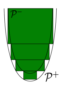
Figure 4. Paraboloids containing/contained in the union of iterated cylinders.

In what follows, $R$ and $r_{0}$ are chosen as functions of $\Delta$. In particular,

$$R\leq\sqrt{\Delta}\quad\text{ and }\quad r_{0}\leq\sqrt{\Delta}.$$

As far as a) is concerned, we should ensure that for all $z\in Q^{-}$ and $r\in(0,r_{0})$,

$$(z\circ r\mathcal{P}^{+})\cap\{t\leq 0\}\subset Q_{1}(0).$$

If $z=(x^{-},v^{-},t^{-})$ and $z^{+}=(x^{+},v^{+},t^{+})\in r\mathcal{P}^{+}$ are such that $z\circ z^{+}\in\{t\leq 0\}$, we have

$$0 \geq t^{-}+t^{+}$$

$$\geq(-\Delta-R^{2})+\frac{4}{3}((4/\omega^{2})\rho^{2}-r^{2})$$

$$\geq-4\Delta+(4^{2}/3\omega^{2})\rho^{2}$$

where $\rho=|v^{+}|$. This implies in particular

$$\rho^{2}\leq\frac{3\omega^{2}}{4}\Delta.$$

In particular, for $\Delta\in(0,1)$,

$$|v^{-}+v^{+}| \leq R+\rho$$

$$\leq(1+\sqrt{3}\omega/2)\sqrt{\Delta}$$

$$|x^{-}+x^{+}+t^{+}v^{-}| \leq R^{3}+\rho^{3}+R$$

$$\leq(1+(\sqrt{3}\omega/2)^{3})\Delta^{3/2}+\sqrt{\Delta}$$

$$\leq(2+(\sqrt{3}\omega/2)^{3})\sqrt{\Delta}.$$

We thus can choose $\Delta$ small enough (recall $\omega=1/\sqrt{5}$) to ensure a).

As far as b) is concerned, notice that for $z^{+}\in Q^{+}$ and $z\in Q^{-}$, we have

$$z^{-1}\circ z^{+}=(t^{+}-t,x^{+}-x-(t^{+}-t)v,v^{+}-v).$$

Choosing $R^{2}\leq\Delta\leq\frac{1}{2}$ we have $2R\leq(4R)^{\frac{1}{3}}$ and we get

$$|v^{+}-v|\leq 2R\leq(4R)^{\frac{1}{3}}$$

$$|x^{+}-x-(t^{+}-t)v|\leq 2R^{3}+(\Delta+R^{2})R=3R^{3}+\Delta R\leq 4R$$

(since $R\leq 1$ and $\Delta\leq 1$) and

$$t^{+}-t\geq\Delta-R^{2}.$$

In particular $z^{-1}\circ z^{+}\in r\mathcal{P}^{-}$ if

$$\Delta-R^{2}\geq\frac{4}{3}\left(\frac{4^{2}}{\omega^{2}}(4R)^{\frac{1}{3}}-r^{2}\right).$$

It is enough satisfy

$$\Delta\geq R^{2}+\frac{4^{3}}{3\omega^{2}}(4R)^{\frac{1}{3}}.$$

Hence, for $\Delta$ given, we can choose $R=R(\Delta)$ small enough to get the desired inequality and in turn point b). ∎

François Golse

École polytechnique, Centre de mathématiques Laurent Schwartz

91128 Palaiseau Cedex, France

e-mail: francois.golse@polytechnique.edu

Cyril Imbert

CNRS & ÉNS, Département de mathématiques et applications

UMR 8553, École normale supérieure (Paris)

45 rue d’Ulm, F-75230 Paris cedex 5, France

e-mail: Cyril.Imbert@ens.fr

Clément Mouhot

University of Cambridge

DPMMS, Centre for Mathematical Sciences

Wilberforce road, Cambridge CB3 0WA, UK

e-mail: C.Mouhot@dpmms.cam.ac.uk

Alexis F. Vasseur

Department of Mathematics, University of Texas at Austin

1 University Station - C1200, Austin, Texas, TX 78712-0257, USA

e-mail: vasseur@math.utexas.edu

References

- [1] Valeri I. Agoshkov. Spaces of functions with differential-difference characteristics and the smoothness of solutions of the transport equation. Dokl. Akad. Nauk SSSR, 276(6):1289–1293, 1984.
- [2] Radjesvarane Alexandre. A review of Boltzmann equation with singular kernels. Kinet. Relat. Models, 2(4):551–646, 2009.
- [3] Radjesvarane Alexandre, Jie Liao, and Chunjin Lin. Some a priori estimates for the homogeneous Landau equation with soft potentials. Kinet. Relat. Models, 8(4):617–650, 2015.
- [4] Radjesvarane Alexandre, Yoshinori Morimoto, Seiji Ukai, Chao-Jiang Xu, and Tong Yang. Regularizing effect and local existence for the non-cutoff Boltzmann equation. Arch. Ration. Mech. Anal., 198(1):39–123, 2010.
- [5] Radjesvarane Alexandre, Yoshinori Morimoto, Seiji Ukai, Chao-Jiang Xu, and Tong Yang. Global existence and full regularity of the Boltzmann equation without angular cutoff. Comm. Math. Phys., 304(2):513–581, 2011.
- [6] Aleksei A. Arsen′ev and Olga E. Buryak. On a connection between the solution of the Boltzmann equation and the solution of the Landau-Fokker-Planck equation. Mat. Sb., 181(4):435–446, 1990.
- [7] François Bouchut. Hypoelliptic regularity in kinetic equations. J. Math. Pures Appl. (9), 81(11):1135–1159, 2002.
- [8] François Bouchut, François Golse, and Mario Pulvirenti. Kinetic equations and asymptotic theory, volume 4 of Series in Applied Mathematics (Paris). Gauthier-Villars, Éditions Scientifiques et Médicales Elsevier, Paris, 2000. Edited and with a foreword by Benoît Perthame and Laurent Desvillettes.
- [9] Luis Caffarelli, Chi Hin Chan, and Alexis Vasseur. Regularity theory for parabolic nonlinear integral operators. J. Amer. Math. Soc., 24(3):849–869, 2011.
- [10] Luis A. Caffarelli and Alexis Vasseur. Drift diffusion equations with fractional diffusion and the quasi-geostrophic equation. Ann. of Math. (2), 171(3):1903–1930, 2010.
- [11] Stephen Cameron, Luis Silvestre, and Stanley Snelson. Global a priori estimates for the inhomogeneous landau equation with moderately soft potentials. Preprint arXiv:1701.08215, 2017.
- [12] Maria C. Caputo and Alexis Vasseur. Global regularity of solutions to systems of reaction-diffusion with sub-quadratic growth in any dimension. Comm. Partial Differential Equations, 34(10-12):1228–1250, 2009.
- [13] Hua Chen, Wei-Xi Li, and Chao-Jiang Xu. Analytic smoothness effect of solutions for spatially homogeneous Landau equation. J. Differential Equations, 248(1):77–94, 2010.
- [14] Yemin Chen, Laurent Desvillettes, and Lingbing He. Smoothing effects for classical solutions of the full Landau equation. Arch. Ration. Mech. Anal., 193(1):21–55, 2009.
- [15] Yemin Chen and Lingbing He. Smoothing estimates for Boltzmann equation with full-range interactions: spatially homogeneous case. Arch. Ration. Mech. Anal., 201(2):501–548, 2011.
- [16] Yemin Chen and Lingbing He. Smoothing estimates for Boltzmann equation with full-range interactions: Spatially inhomogeneous case. Arch. Ration. Mech. Anal., 203(2):343–377, 2012.
- [17] Ennio De Giorgi. Sull’analiticità delle estremali degli integrali multipli. Atti Accad. Naz. Lincei. Rend. Cl. Sci. Fis. Mat. Nat. (8), 20:438–441, 1956.
- [18] Ennio De Giorgi. Sulla differenziabilità e l’analiticità delle estremali degli integrali multipli regolari. Mem. Accad. Sci. Torino. Cl. Sci. Fis. Mat. Nat. (3), 3:25–43, 1957.
- [19] Laurent Desvillettes. About the regularizing properties of the non-cut-off Kac equation. Comm. Math. Phys., 168(2):417–440, 1995.
- [20] Laurent Desvillettes. Plasma kinetic models: the Fokker-Planck-Landau equation. In Modeling and computational methods for kinetic equations, Model. Simul. Sci. Eng. Technol., pages 171–193. Birkhäuser Boston, Boston, MA, 2004.
- [21] Laurent Desvillettes. Entropy dissipation estimates for the Landau equation in the Coulomb case and applications. J. Funct. Anal., 269(5):1359–1403, 2015.
- [22] Laurent Desvillettes and Cédric Villani. On the spatially homogeneous Landau equation for hard potentials. I. Existence, uniqueness and smoothness. Comm. Partial Differential Equations, 25(1-2):179–259, 2000.
- [23] Laurent Desvillettes and Cédric Villani. On the spatially homogeneous Landau equation for hard potentials. II. -theorem and applications. Comm. Partial Differential Equations, 25(1-2):261–298, 2000.
- [24] Emmanuele DiBenedetto. On the local behaviour of solutions of degenerate parabolic equations with measurable coefficients. Ann. Scuola Norm. Sup. Pisa Cl. Sci. (4), 13(3):487–535, 1986.
- [25] Emmanuele DiBenedetto, Ugo Gianazza, and Vincenzo Vespri. Forward, backward and elliptic Harnack inequalities for non-negative solutions to certain singular parabolic partial differential equations. Ann. Sc. Norm. Super. Pisa Cl. Sci. (5), 9(2):385–422, 2010.
- [26] Emmanuele DiBenedetto, Ugo Gianazza, and Vincenzo Vespri. Harnack type estimates and Hölder continuity for non-negative solutions to certain sub-critically singular parabolic partial differential equations. Manuscripta Math., 131(1-2):231–245, 2010.
- [27] Emmanuele DiBenedetto, Ugo Gianazza, and Vincenzo Vespri. Harnack’s inequality for degenerate and singular parabolic equations. Springer Monographs in Mathematics. Springer, New York, 2012.
- [28] Ron J. DiPerna and Pierre-Louis Lions. Global weak solutions of Vlasov-Maxwell systems. Comm. Pure Appl. Math., 42(6):729–757, 1989.
- [29] Matthieu Felsinger and Moritz Kassmann. Local regularity for parabolic nonlocal operators. Comm. Partial Differential Equations, 38(9):1539–1573, 2013.
- [30] M. Giaquinta and E. Giusti. Partial regularity for the solutions to nonlinear parabolic systems. Ann. Mat. Pura Appl. (4), 97:253–266, 1973.
- [31] M. Giaquinta and G. Modica. Regularity results for some classes of higher order nonlinear elliptic systems. J. Reine Angew. Math., 311/312:145–169, 1979.
- [32] Mariano Giaquinta and Michael Struwe. On the partial regularity of weak solutions of nonlinear parabolic systems. Math. Z., 179(4):437–451, 1982.
- [33] François Golse and Alexis F. Vasseur. Hölder regularity for hypoelliptic kinetic equations with rough diffusion coefficients, 2015. Version 2.
- [34] François Golse, Pierre-Louis Lions, Benoît Perthame, and Rémi Sentis. Regularity of the moments of the solution of a transport equation. J. Funct. Anal., 76(1):110–125, 1988.
- [35] François Golse, Benoît Perthame, and Rémi Sentis. Un résultat de compacité pour les équations de transport et application au calcul de la limite de la valeur propre principale d’un opérateur de transport. C. R. Acad. Sci. Paris Sér. I Math., 301(7):341–344, 1985.
- [36] Thierry Goudon and Alexis Vasseur. Regularity analysis for systems of reaction-diffusion equations. Ann. Sci. Éc. Norm. Supér. (4), 43(1):117–142, 2010.
- [37] Philip T. Gressman, Joachim Krieger, and Robert M. Strain. A non-local inequality and global existence. Adv. Math., 230(2):642–648, 2012.
- [38] Philip T. Gressman and Robert M. Strain. Global classical solutions of the Boltzmann equation without angular cut-off. J. Amer. Math. Soc., 24(3):771–847, 2011.
- [39] Maria Gualdani and Nestor Guillen. Estimates for radial solutions of the homogeneous Landau equation with Coulomb potential. Anal. PDE, 9(8):1772–1809, 2016.
- [40] Yan Guo. The Landau equation in a periodic box. Comm. Math. Phys., 231(3):391–434, 2002.
- [41] Yan Guo. The Vlasov-Poisson-Boltzmann system near Maxwellians. Comm. Pure Appl. Math., 55(9):1104–1135, 2002.
- [42] Lars Hörmander. Hypoelliptic second order differential equations. Acta Math., 119:147–171, 1967.
- [43] Cyril Imbert and Clément Mouhot. Hölder continuity of solutions to hypoelliptic equations with bounded measurable coefficients. Technical report, arXiv:1505.04608, 2015. Version 5.
- [44] Cyril Imbert and Luis Silvestre. An introduction to fully nonlinear parabolic equations. In An introduction to the Kähler-Ricci flow, volume 2086 of Lecture Notes in Math., pages 7–88. Springer, Cham, 2013.
- [45] Moritz Kassmann. A priori estimates for integro-differential operators with measurable kernels. Calc. Var. Partial Differential Equations, 34(1):1–21, 2009.
- [46] Andrei Kolmogoroff. Zufällige Bewegungen (zur Theorie der Brownschen Bewegung). Ann. of Math. (2), 35(1):116–117, 1934.
- [47] Joachim Krieger and Robert M. Strain. Global solutions to a non-local diffusion equation with quadratic non-linearity. Comm. Partial Differential Equations, 37(4):647–689, 2012.
- [48] Olga A. Ladyzhenskaya and Nina N. Ural′tseva. Linear and quasilinear elliptic equations. Translated from the Russian by Scripta Technica, Inc. Translation editor: Leon Ehrenpreis. Academic Press, New York-London, 1968.
- [49] Pierre-Louis Lions. On Boltzmann and Landau equations. Philos. Trans. Roy. Soc. London Ser. A, 346(1679):191–204, 1994.
- [50] Shuangqian Liu and Xuan Ma. Regularizing effects for the classical solutions to the Landau equation in the whole space. J. Math. Anal. Appl., 417(1):123–143, 2014.
- [51] Jürgen Moser. A Harnack inequality for parabolic differential equations. Comm. Pure Appl. Math., 17:101–134, 1964.
- [52] John F. Nash. Continuity of solutions of parabolic and elliptic equations. Amer. J. Math., 80:931–954, 1958.
- [53] Andrea Pascucci and Sergio Polidoro. The Moser’s iterative method for a class of ultraparabolic equations. Commun. Contemp. Math., 6(3):395–417, 2004.
- [54] Linda Preiss Rothschild and E. M. Stein. Hypoelliptic differential operators and nilpotent groups. Acta Math., 137(3-4):247–320, 1976.
- [55] Luis Silvestre. Upper bounds for parabolic equations and the Landau equation. Technical report, arxiv 1511.03248, 2016. Version 2.
- [56] Michael Struwe. On the Hölder continuity of bounded weak solutions of quasilinear parabolic systems. Manuscripta Math., 35(1-2):125–145, 1981.
- [57] Alexis Vasseur. Higher derivatives estimate for the 3D Navier-Stokes equation. Ann. Inst. H. Poincaré Anal. Non Linéaire, 27(5):1189–1204, 2010.
- [58] Alexis F. Vasseur. The De Giorgi method for elliptic and parabolic equations and some applications. Preprint, to appear in Lectures on the Analysis of Nonlinear Partial Differential Equations Vol. 4.
- [59] Cédric Villani. On the spatially homogeneous Landau equation for Maxwellian molecules. Math. Models Methods Appl. Sci., 8(6):957–983, 1998.
- [60] WenDong Wang and LiQun Zhang. The regularity of a class of non-homogeneous ultraparabolic equations. Sci. China Ser. A, 52(8):1589–1606, 2009.
- [61] Wendong Wang and Liqun Zhang. The regularity of weak solutions of ultraparabolic equations. Discrete Contin. Dyn. Syst., 29(3):1261–1275, 2011.
- [62] Kung-Chien Wu. Global in time estimates for the spatially homogeneous Landau equation with soft potentials. J. Funct. Anal., 266(5):3134–3155, 2014.