Free boundary problems
in PDEs and particle systems

G. Carinci, A. De Masi, C. Giardinà, E. Presutti

Free boundary problems
in PDEs and particle systems

Chapter 1 Introduction

We develop here a theory for free boundary problems which applies to a large class of systems arising from problems in various, even distant, areas of research and which share a common mathematical structure. As we shall see in some detail, these are models for heat conduction, queuing theory, propagation of fire, interface dynamics, population dynamics and evolution of biological systems with selection mechanisms. We shall consider models in continuum and interacting particle systems. Their common mathematical features are the following:

(1) Microscopic particle dynamics stem from interactions of topological nature.
(2) Macroscopic evolution is ruled by a free boundary problem.

In fact in the models we consider the particles move in $d=1$ dimension so that there is a rightmost and a leftmost particle, called boundary particles. The rules of dynamics are the usual ones, particles are either free (independent random walks or Brownian motions) or they have some local interaction (for instance simple exclusion) and on top of that there may be creations of new particles or particles may duplicate via a branching process. In addition, in order to keep (approximatively) constant the total number of particles, boundary particles are subject to a death process.

The topological nature of the interaction refers to the fact that the boundary particles are special as they may disappear at some given rate, being then replaced by new boundary particles, the rightmost and leftmost particles among those which have survived. Thus the “inside particles”, i.e. those in between the boundary particles, evolve in the “usual” way, but the inside particles are not fixed a priori and may eventually become boundary particles depending on the evolution itself.

As a consequence of particle evolution, the spatial domain occupied by the particles varies in time. In particular the location of the boundary particles changes in the course of time due to the death process at the boundary. Correspondingly, as we shall discuss extensively in this volume, the macroscopic version of the models is provided by a free boundary problem for a PDE with Dirichlet condition supplemented by prescribing the boundary flux. As often occurs, one can relate a macroscopic evolution to microscopic dynamics via a scaling limit procedure (hydrodynamic limit).

The basic example that we will study in detail here is given by the linear heat equation

$$\frac{\partial\rho}{\partial t}=\frac{1}{2}\frac{\partial^{2}\rho}{\partial r^{2}}$$

in the time varying domain $[0,X_{t}]$ with some initial condition $\rho(r,0)=\rho_{0}(r)\geq 0$ and boundary conditions

$$-\frac{1}{2}\frac{\partial\rho}{\partial r}(0,t)=j>0,\quad\rho(X_{t},t)=0\;.$$

The free boundary $X_{t}$ (also called the edge in this book) is not given a priori but it should be determined in such a way that

$$-\frac{1}{2}\frac{\partial\rho}{\partial r}(X_{t},t)=j.$$

Interpreting $\rho$ as a mass density, the last condition states that the mass flux leaving the system at $X_{t}$ must be equal to $j$, and since $j$ is also the mass flux entering at 0 (as fixed by the boundary condition at 0), the total mass in the system is preserved. From this perspective the free boundary problem becomes a control problem: find an edge evolution $X_{t}$ in such a way that the total mass is constant in time.

Well known theorems on the Stefan problem yield a local existence theorem for our basic example when we have “classical initial data”. We will define here a weak version of the problem and prove global existence and uniqueness of a relaxed solution for general initial data. The other models that we will consider in this work have similar structure and the strategies of proof are very close to that in the basic example. The key point in all of them is:

Construct upper and lower barriers that squeeze the solution we are looking for.

The correct notion of order for these problems is defined by mass transport. Referring to a basic example for the sake of definiteness, the barriers are defined in terms of a simplified evolution where we introduce a time grid of length $\delta$ and the evolution is ruled by the heat equation in $\mathbb{R}_{+}$ in the open intervals $(n\delta,(n+1)\delta)$ with boundary condition

$$-\frac{1}{2}\frac{\partial\rho}{\partial r}(0,t)=j\;.$$

At the times $n\delta$ we remove an amount of mass equal to $j\delta$ so that at these times the mass conservation is restored. The key point is that we get an upper barrier if we start by removing mass already at time 0 while we get a lower barrier when we remove mass from time $\delta$ on: the order here is in the sense of moving mass to the right. A key step is to prove that the barriers have a unique separating element. Once we have this we conclude by showing that the solution we are considering is trapped in between the barriers which then identifies the solution as the element separating the barriers. As we will see this part of the proof exploits extensively probabilistic ideas and techniques based on the well known relation between heat equation and Brownian motion and between the hitting distribution at the boundaries and the Dirichlet condition in the heat equation.

We think it can be useful for the reader to have one case worked out in all details, so that in Part I we prove the above in the context of our basic example by proving global existence and uniqueness of the relaxed solution of the problem; we also show that this is the limit of the empirical mass density of the associated particle system (in the hydrodynamic limit). In Part II we discuss, in a very sketchy way, several other models, the conjecture being that the results proved for the basic model extend to these other cases that have been done, at least partially.

Part I The basic model

Chapter 2 Introduction to Part I

In Part I of this work we study a model for mass transport where Fick’s law is satisfied. Fick’s law is the analogue for mass of Fourier’s law for heat conduction. Fourier’s law, see [29], specifies the amount of heat flux in a metal bar when we heat it from one side and cool it from the other. Its analogue for mass fluxes is Fick’s law, formally described by the same equation. Since the transversal direction to the flow is not relevant we model our system as one dimensional. The ideal experiment of mass transport that we have in mind is the following: for $t\geq 0$ we confine the system in a time varying space interval $[0,X_{t}]$, where $X_{t}$ is a given positive, continuous and piecewise $C^{1}$ function; for instance we move the edge $X_{t}$ with constant velocity for some time, then we change velocity and so on. We act on the system by injecting mass from its left boundary 0 at rate $j>0$ while we remove mass from the right boundary $X_{t}$ in such a way as to keep the mass density at $X_{t}$ equal to 0 for all $t\geq 0$. The evolution of the mass density $\rho(r,t)$ in the interior of the spatial domain is ruled by combining the continuity equation and Fick’s law, so that, supposing a constant conductivity (set equal to 1/2), we have

$$\frac{\partial\rho}{\partial t}=-\frac{\partial J}{\partial r}\;,\qquad J=-\frac{1}{2}\frac{\partial\rho}{\partial r}$$ (0.1)

where $J(r,t)$ is the local mass-flux and $\rho(r,t)$ the mass density. Thus $\rho(r,t)$ solves the heat equation

$$\frac{\partial\rho}{\partial t}=\frac{1}{2}\frac{\partial^{2}\rho}{\partial r^{2}}$$ (0.2)

in the time varying domain $[0,X_{t}]$ with some initial condition $\rho(r,0)=\rho_{0}(r)$ and boundary conditions

$$J(0,t)=j,\quad\rho(X_{t},t)=0\;.$$ (0.3)

Physically these boundary conditions mean that the system is in contact with a current reservoir which sends in mass at rate $j$ and thus imposes a current $j$ at the origin; instead at the other endpoint $X_{t}$ there is a density reservoir which removes mass as fast as needed to fix the mass density to be constantly equal to zero. As a consequence, in this setting, the total mass of the system is not a conserved quantity.

The main question we want to study here arises when we require mass conservation at all times. To achieve this, one needs to regard $X_{t}$ as a control parameter and one is lead to study the following control problem:

Is it possible to choose $X_{t}$ in such a way that the total mass in the system is constant ?

We clearly succeed if we can solve the free boundary problem (FBP) given by (0.2) with initial datum $\rho(r,0)=\rho_{0}(r)$, $r\in[0,X_{0}]$, and

$$-\frac{1}{2}\frac{\partial\rho}{\partial r}(0,t)=j,\qquad-\frac{1}{2}\frac{\partial\rho}{\partial r}(X_{t},t)=j,\qquad\rho(X_{t},t)=0\;.$$ (0.4)

In fact the rate at which mass is taken out of the system from $X_{t}$ is

$$J(X_{t},t)=-\frac{1}{2}\frac{\partial\rho}{\partial r}(X_{t},t)$$

which, by (0.4), is exactly equal to the rate at which we inject mass at $0$ so that the total mass is constant.

As discussed in the next chapter (see Section 3) we can find in the existing literature on FBP an affirmative answer for special initial data and for finite times. In fact one can readily check (see Section 3 for details) that the current $J(r,t)$ solves the classical Stefan problem for which the theory (in particular in one dimension) is very rich with many detailed results available [19, 20, 27, 36, 44]. As a consequence local existence and uniqueness of classical solutions can be proved for the FBP (0.2)–(0.4) for smooth initial data which satisfy the boundary conditions. In some cases the classical solution is global extending to all times, but this is not true in general as it is known that singularities may develop.

Thus our control problem when stated for an arbitrarily long time interval $[0,T]$ and for general initial data cannot always be solved via the above FBP. Take for instance $\rho_{0}\in L^{1}(\mathbb{R}_{+})$, bounded, continuous and everywhere strictly positive: in such a case the whole problem has to be redefined. As usual the idea is to study a relaxed version: we thus introduce an accuracy parameter $\epsilon>0$ and replace $\rho_{0}$ by a nice function $\rho^{(\epsilon)}_{0}$, smooth, non-negative and with compact support, requiring however that $\int|\rho_{0}(r)-\rho^{(\epsilon)}_{0}(r)|\;dr\leq\epsilon$. We may also ask that $\rho^{(\epsilon)}_{0}$ satisfies (0.4) so that, for what said above, we have a classical solution of FBP for some time $[0,S]$. However this could be shorter than the interval $[0,T]$ we have fixed initially, in which case the problem still remains. Moreover even if $S\geq T$ we have a poor control of the solution and it is hard to see how this behaves when we remove the relaxation taking $\epsilon\to 0$. The idea then is to further simplify the problem by relaxing also the boundary condition at the edge. We refer to the next chapter for a precise definition. Here we just say that in Part I we will prove that any $\epsilon$-relaxed solution converges to a unique limit when $\epsilon\to 0$. This will allow us to define a notion of relaxed solution of the problem which is global in time and applies to a large class of initial data.

In the last chapter of Part I we study a particles version of the above basic model. The system has $N$ particles so that the mass distribution is no longer continuous but instead concentrated on points (the positions of the $N$ particles). To simulate an initial condition $\rho_{0}(r)$ (we assume $\int\rho_{0}(r)dr=1$ for simplicity), we distribute the $N$ particles independently of each other and with law $\rho_{0}(r)dr$. We then define the “empirical mass density measure”

$$\pi_{0}^{(N)}(dr)=\frac{1}{N}\sum_{i=1}^{N}\delta_{B_{i}(0)}(r)dr$$ (0.5)

where $B_{i}(0)$ are the random positions of the $N$ particles and $\delta_{a}(r)$ is the Dirac delta at $a$. The value $0$ refers to time, so far we have been describing the situation at time 0. Thus $\pi_{0}^{(N)}(dr)$ is a probability measure on $\mathbb{R}$ which is random as the terms $B_{i}(0)$ are the random positions of the particles. If we denote by $E$ the expectation with respect to the law of the $B_{i}(0)$ and by $f(r)$ a test function, we have

$$E\Big{[}\int\pi_{0}^{(N)}(dr)f(r)\Big{]}=\int\rho_{0}(r)f(r)dr.$$ (0.6)

By the law of large number if $N$ is large we do not need to take the expectation because, with large probability, $\int\pi_{0}^{(N)}(dr)f(r)$ is close to $\int\rho_{0}(r)f(r)dr$.

Let us now make the particles move. We first consider the free case where the particles are independent Brownian motions $B_{i}(t)$ on $\mathbb{R}_{+}$ with reflection at 0. Call $\pi_{t}^{(N)}(dr)$ the random mass distribution at time $t$ and denote now by $E$ the joint law of the initial distribution of the particles and of their Brownian evolution. We then have

$$E\Big{[}\int\pi_{t}^{(N)}(dr)f(r)\Big{]}=\int\rho(r,t)f(r)dr$$ (0.7)

where $\rho(r,t)$ is the solution of (0.2) on $\mathbb{R}_{+}$ with Neumann boundary condition at 0 given by $\frac{\partial\rho}{\partial r}(0,t)=0$. All that is the well known relation between heat equation and Brownian motions.

We next go to the injection-removal of mass mechanism. This is simply done as follows: at exponential times of intensity $jN$ the rightmost particle moves to the origin (which is the same as saying that we add a new Brownian particle at 0 and simultaneously we take out the particle which at that time is the rightmost one). In between such actions the particles move as independent Brownian motions (with reflection at the origin). We denote again by $E$ the expectation with respect to the law of this process (which includes the initial distribution of the particles, their motion and the injection-removal of particles). Thus the total mass (i.e. the total number of particles) is conserved but as in the continuum we are injecting mass at 0 and removing mass on the right. Such a simple action however creates strong correlations among the particles: the choice of the rightmost particle requires knowledge of the positions of all the others. We thus lose the independency property and the analysis of the left-hand side of (0.7) in this case becomes highly non-trivial. Existence of the process is easy but the relation with the continuum version is harder. The question becomes simpler if we study the asymptotic behavior of the system as $N\to\infty$, namely its “hydrodynamic limit”. We would like that:

$$\lim_{N\to\infty}E\Big{[}\int\pi_{t}^{(N)}(dr)f(r)\Big{]}=\int\rho(r,t)f(r)dr$$ (0.8)

where $\rho(r,t)$ is the solution of the control problem described previously and in particular of the FBP when this has a classical solution. In Chapter 11 we prove (0.8).

Chapter 3 The basic model, definitions and results

In this chapter we expand the analysis presented in the Introduction by giving a detailed definition of the control problem and its relaxed version. We then show that for special initial conditions the control problem is related to a free boundary problem (FBP) which is solved locally in time using the existing literature on the Stefan problem. We then present the main result of Part I (Theorem 4.1) which states that the relaxed control problem has a unique global solution. The proof uses inequalities based on mass transport. We introduce lower and upper barriers obtained by a time discretization of (0.2)–(0.3) and state the other main theorem of Part I (Theorem 14), which says that there is a unique element which separates the lower and upper barriers. The proof of Theorem 14 starts in Chapter 4 and is completed in Chapter 7. The proof of Theorem 4.1 is carried out in the remaining chapters of Part I, the essential point is to show that the elements of an optimal sequence are eventually squeezed between the barriers and therefore their limit points coincide with the unique element which separates the barriers.

1 The basic problem

As discussed in the Introduction we consider the heat equation (0.2) in the time varying domain $[0,X_{t}]$, $X_{t}$ a positive, continuous and piecewise $C^{1}$ function, with boundary conditions (0.3) and initial datum $\rho_{0}$.

Definition 3.1 (Assumptions on $\rho_{0}$)

We suppose throughout the sequel that $\rho_{0}(r)$ is a non-negative function belonging to the set

$$\mathcal{U}=\left\{u\in L^{\infty}(\mathbb{R}_{+},\mathbb{R}_{+})\cap L^{1}(\mathbb{R}_{+},\mathbb{R}_{+})\;:\;\int u>0\right\}.$$ (1.1)

Definition 3.2 (The basic problem)

The function $\rho(r,t)$ is a solution of the basic problem in the time interval $[0,T]$ with initial datum $\rho_{0}$ if there exists $X_{t}$ positive so that $\rho(r,t)$ solves (0.2)–(0.3) with initial condition $\rho_{0}$ and

$$\int_{0}^{X_{t}}\rho(r,t)\,dr=\int_{0}^{X_{0}}\rho_{0}(r)\,dr\quad\text{for all $t>0$}.$$ (1.2)

Definition 3.3 (The $\epsilon$-relaxed problem)

For $\epsilon>0$, the function $\rho^{(\epsilon)}(r,t)$ is a $\epsilon$-relaxed solution of the basic problem with initial datum $\rho_{0}$ in the time interval $[0,T]$ if

• $\int|\rho_{0}(r)-\rho^{(\epsilon)}(r,0)|dr\leq\epsilon$,

• there exists $X^{(\epsilon)}_{t}$, $t\in[0,T]$, positive, continuous and piecewise $C^{1}$ so that for each $t\in[0,T]$, $\rho^{(\epsilon)}(r,t)$ has support in $[0,X^{(\epsilon)}_{t}]$,

• $\rho^{(\epsilon)}(r,t)$ solves (0.2)–(0.3) in $[0,T]$ with $X_{t}$ replaced by $X^{(\epsilon)}_{t}$ and with initial condition $\rho^{(\epsilon)}(r,0)$,

• approximate mass conservation is satisfied, i.e.

  $$\Big{|}\int_{0}^{X^{(\epsilon)}_{t}}\rho^{(\epsilon)}(r,t)\,dr-\int_{0}^{X^{(\epsilon)}_{0}}\rho^{(\epsilon)}_{0}(r)\,dr\Big{|}\leq\epsilon\quad\text{for all $t\in[0,T]$}.$$ (1.3)

Definition 3.4 (Optimal sequences)

The sequence $\rho^{(\epsilon_{n})}(r,t)$ is an optimal sequence relative to $\rho_{0}$ and $T>0$ if for each $n\in\mathbb{N}$ the function $\rho^{(\epsilon_{n})}(r,t)$ is an $\epsilon_{n}$-relaxed solution in $[0,T]$ of the basic problem with initial datum $\rho_{0}$ and if $\epsilon_{n}\to 0$ as $n\to\infty$.

Definition 3.5 (Relaxed solution)

$\rho(r,t)$ is a relaxed solution in $[0,T]$ of the basic problem with initial datum $\rho_{0}$ if it is a weak limit of the elements $\rho^{(\epsilon_{n})}(r,t)$ of an optimal sequence in $[0,T]$ with initial datum $\rho_{0}$.

2 Stationary solutions

The basic problem (see Definition 3.2) has special global solutions given by the stationary profiles:

$$\rho^{(st)}(r|M)=\Big{(}a(M)-2jr\Big{)}\mathbf{1}_{a(M)-2jr\geq 0},\qquad\int\rho^{(st)}(r|M)dr=M$$ (2.1)

Since mass is conserved we have a one parameter family of stationary solutions indexed by the mass (denoted above by $M$). We conjecture that these are the only stationary solutions but we do not have a proof.

In many problems stationary profiles are helpful because they can be used to “trap” trajectories and thus give a-priori estimates. We will prove that the relaxed solutions of the basic problem (see Definition 3.5) preserve order and this together with the knowledge of the stationary solutions will play an important role in the sequel.

3 The FBP for the basic model

$\rho_{0}$ is a classical initial datum if it is a smooth, strictly positive function in $[0,X_{0})$, $X_{0}>0$, and it is such that

$$\lim_{r\to X_{0}}\rho_{0}(r)=0,\quad\lim_{r\to 0}\frac{d\rho_{0}(r)}{dr}=-2j,\;\lim_{r\to X_{0}}\frac{d\rho_{0}(r)}{dr}=-2j.$$ (3.1)

Theorem 3.1 (Local classical solutions).

If $\rho_{0}$ is a classical initial datum then the basic problem (of Definition 3.2) has a local solution: namely there exists $T>0$ and $\{X_{t},t\in[0,T]\}$, so that (0.2) with initial datum $\rho_{0}$ has a solution $\rho(r,t)$ which satisfies (0.4) for all $t\in[0,T]$. If $v(r,0):=-\frac{1}{2}\frac{\partial\rho_{0}}{\partial r}(r)-j\geq 0$ then the local solution extends to all times.

The proof of Theorem 3.1 given below follows from the theory of the Stefan problem as we are going to see. The equations (0.2) and (0.4) complemented by the initial datum $\rho_{0}$ in the unknowns $X_{t}$, and $\rho(\cdot,t)$ define a free boundary problem, FBP, where the datum at the free boundary involves both the value of $\rho$ and its space derivative. In the Stefan problem, the prototype of FBP’s, instead the datum is the speed of the edge:

$$\frac{\partial v}{\partial t}=\frac{1}{2}\frac{\partial^{2}v}{\partial r^{2}}\;\;\quad v(r,t)\Big{|}_{r=0,X_{t}}=0,$$ (3.2)

$$\frac{dX_{t}}{dt}=-(2j)^{-1}\frac{\partial v(r,t)}{\partial r}\Big{|}_{r=X_{t}}.$$

Local existence for (3.2) is proved in [20]–[24].

Proof of Theorem 3.1.Given $X_{t}$ and $v(r,t)$ satisfying (3.2) we set

$$\rho(r,t)=2\int_{r}^{X_{t}}\Big{(}v(r^{\prime},t)+j\Big{)}dr^{\prime}.$$ (3.3)

One can then check that (0.2) and (0.4) are all satisfied. The non-negativity of $\rho(\cdot,t)$ follows from the maximum principle. Following Fasano and Primicerio, see e.g. [20], we say that if $v(r,0)\geq 0$ then (3.2) has a “sign specification”. With a sign specification the solution is global hence the last statement in Theorem 3.1. ∎

Uniqueness of the local classical solution for the Stefan problem (3.2) is also known. As mentioned if there is a sign specification the solution of (3.2) is global while if there is no sign specification in general we only have local existence with examples where singularities do appear. The analysis of their structure is a very interesting and much studied problem, see for instance [10], [25], [26], [39].

4 Main theorem: existence and uniqueness

By default throughout this chapter the initial datum $\rho_{0}\in\mathcal{U}$, see Definition 3.1.

Theorem 4.1 (Existence and uniqueness).

Let $\rho_{0}\in\mathcal{U}$, then for any $T>0$ there exists a unique relaxed solution of the basic problem in $[0,T]$ with initial datum $\rho_{0}$ (see Definition 3.5). Moreover:

• As implicit in the above statement there exist optimal sequences in $[0,T]$ with initial datum $\rho_{0}$.

• The elements $\rho^{(\epsilon_{n})}(r,t)$ of an optimal sequence relative to $\rho_{0}$ and $T>0$, converge weakly to a limit $\rho_{T}(r,t)$.

• The limit $\rho_{T}(r,t)$ is independent of the optimal sequence and if $S>T$, $\rho_{S}(r,t)=\rho_{T}(r,t)$, $t\in[0,T]$. We denote by $\rho(r,t)$ the function which agrees with $\rho_{T}(r,t)$ for all $T>0$.

• For all $t>0$ $\rho(r,t)$ is in $L^{1}$ and $\int\rho(r,t)dr=\int\rho_{0}(r)dr$.

• If $\rho_{0}\leq\rho^{*}_{0}$ then $\rho(r,t)\leq\rho^{*}(r,t)$.

• $\rho(r,t)$ converges weakly to $\rho_{0}$ as $t\to 0$.

Moreover, if $\rho_{0}(r)$ is continuous and with support in $[0,X_{0}]$, then

• $\rho(r,t)$ is a continuous function in $(r,t)$ which converges pointwise to $\rho_{0}$ as $t\to 0$.

• If $\rho_{0}$ is a classical initial datum $\rho(r,t)$ solves the FBP of Section 3 locally in time.

Since any classical solution $\{(X_{t},\rho(\cdot,t)),t\in[0,T]\}$, of the FBP (0.2)–(0.4) is also an optimal sequence, (choosing $X^{(\epsilon)}_{t}=X_{t}$ and $\rho^{(\epsilon_{n})}(r,t)=\rho(r,t)$ for any $n$), then $\rho(\cdot,t)$ coincides with the function defined in Theorem 4.1 and item (h) follows.

The weak point in the above theorem is the lack of control of the edge. We have only what was stated in the following Corollary which is an immediate consequence of item (e) of Theorem 4.1 and of the existence of a stationary solution of the classical FBP as discussed in Section 2. Recall (2.1) for notation.

Corollary 6

If $\rho^{(st)}(r|M^{\prime})\leq\rho_{0}(r)\leq\rho^{(st)}(r|M^{\prime\prime})$ then

$$\rho^{(st)}(r|M^{\prime})\leq\rho(r,t)\leq\rho^{(st)}(r|M^{\prime\prime})\quad\text{for all $t>0$}.$$ (4.1)

In particular if $\rho_{0}(r)$ has compact support then there exists $X>0$ so that $\rho(r,t)=0$ for all $r\geq X$.

We will prove Theorem 4.1 using a variational method which is explained in the next sections.

5 The upper and lower barriers

We do not have enough information on the elements $\rho^{(\epsilon_{n})}(r,t)$ in an optimal sequence to directly prove that they converge as $\epsilon_{n}\to 0$. We will instead introduce a different relaxation procedure where the removal of mass occurs only at discrete times $n\delta$, $n\in\mathbb{N}$, $\delta>0$. The evolution in the time intervals $(n\delta,(n+1)\delta)$ is free, namely given by (0.2) with only the boundary condition at $0$, i.e. the first one in (0.3), the other one at $X_{t}$ is dropped. Therefore in these time intervals the mass density is strictly positive on the whole $\mathbb{R}_{+}$. At the times $n\delta$ we remove the right amount of mass, equal to $j\delta$, by cutting the right part of the function which after the cut has compact support. Such evolutions are much simpler than those in the optimal sequence but they have also the extra advantage of monotone properties, this is why we call them upper and lower barriers. Monotonicity will allow us to control the limit as $\delta$ goes to 0 of the barriers and then to relate this to the limit of the $\rho^{(\epsilon_{n})}(r,t)$. We start here with the definition of the barriers.

To this end we introduce a time mesh $\delta>0$ and will define the barriers at the times $k\delta$, $k\geq 0$. We use the following notation:

$$\mathcal{U}_{\delta}=\{u\in\mathcal{U}:\int u>j\delta\}$$ (5.1)

where $\mathcal{U}$ has been defined in (1.1), and we introduce two operators, i.e. the cut operator $C_{\delta}$ on $\mathcal{U}_{\delta}$ and the free evolution operator $T_{\delta}$ on $\mathcal{U}$.

Definition 7 (The cut operator)

The cut operator $C_{\delta}$ maps $u\in\mathcal{U}_{\delta}$ into $\mathcal{U}$ as follows:

$$C_{\delta}u(r)=\mathbf{1}_{r\leq R_{u}}u(r),\quad\text{where}\quad R_{u}:\;\;\int_{R_{u}}^{\infty}u(r)dr=j\delta.$$ (5.2)

Observe that $\int C_{\delta}u=\int u-j\delta$.

To define the free evolution operator we use the Green functions:

Definition 8 (The Green function)

Define for $r$, $r^{\prime}$ and $t>s\geq 0$ the Green function

$$G_{s,t}^{\rm neum}(r^{\prime},r)=G_{t-s}(r^{\prime},r)+G_{t-s}(r^{\prime},-r),\quad G_{t}(r^{\prime},r)=\frac{e^{-\frac{(r-r^{\prime})^{2}}{2t}}}{\sqrt{2\pi t}}$$ (5.3)

and write for any $u\in\mathcal{U}$:

$$G_{s,t}^{\rm neum}*u(r)=\int_{\mathbb{R}_{+}}G_{s,t}^{\rm neum}(r^{\prime},r)u(r^{\prime})\,dr^{\prime}.$$ (5.4)

To simplify notation we shall sometimes write

$$G_{t-s}^{\rm neum}(r^{\prime},r)=G_{s,t}^{\rm neum}(r^{\prime},r).$$ (5.5)

The following proposition explains why $G_{t}^{\rm neum}$ is called the Green function.

Proposition 9.

The function $(r,t)\mapsto G_{t}^{\rm neum}(r^{\prime},r)$, $t>0$, $r^{\prime},r>0$, solves the heat equation (0.2) and for any $t>0$,

$$\lim_{r\to 0}\frac{\partial}{\partial r}G_{t}^{\rm neum}(r^{\prime},r)=0.$$

Moreover if $u\in\mathcal{U}$ is a continuous function

$$T_{t}u(r):=G_{t}^{\rm neum}*u(r)+j\int_{0}^{t}G_{s^{\prime},t}^{\rm neum}(0,r)\,ds^{\prime}$$ (5.6)

solves (0.2), converges to $u(r)$ as $t\to 0$ and for any $t>0$

$$\lim_{r\to 0}\frac{\partial}{\partial r}T_{t}u(r)=-2j.$$ (5.7)

Proof. The above statements are direct consequence of the following properties of the Gaussian kernel. For $t>0$:

$$\Big{(}\frac{\partial}{\partial t}-\frac{1}{2}\frac{\partial^{2}}{\partial r^{2}}\Big{)}\frac{e^{-r^{2}/2t}}{\sqrt{2\pi t}}=0,$$ (5.8)

$$\lim_{t\to 0^{+}}\int_{-\epsilon}^{\epsilon}\frac{e^{-x^{2}/2t}}{\sqrt{2\pi t}}dx=1,\quad\text{for any $\epsilon>0$},$$ (5.9)

$$\lim_{x\to 0^{+}}\int_{0}^{t}\frac{x}{t-s}\frac{e^{-x^{2}/2(t-s)}}{\sqrt{2\pi(t-s)}}ds=1.$$ (5.10)

∎

We are now ready for the definition of the free evolution operator:

Definition 10 (The free evolution operator)

The free evolution operator $T_{\delta}$ maps $\mathcal{U}$ into itself and $T_{\delta}u$ is equal to the expression (5.6) with $t=\delta$.

It follows directly from the definition that:

$$\int T_{\delta}u=j\delta+\int u$$ (5.11)

and therefore that the products

$$C_{\delta}T_{\delta} T_{\delta}C_{\delta}$$ and preserve the mass (5.12)

(the latter defined on $\mathcal{U}_{\delta}$ ).

Definition 11 (The barriers)

The upper barrier $S^{\delta,+}_{k\delta}u$, $k\geq 0$, is defined as

$$S^{\delta,+}_{k\delta}u=(T_{\delta}C_{\delta})^{k}u,\quad u\in\mathcal{U}_{\delta}$$ (5.13)

while the lower barrier $S^{\delta,-}_{k\delta}u$, $k\geq 0$, is

$$S^{\delta,-}_{k\delta}u=(C_{\delta}T_{\delta})^{k}u,\quad u\in\mathcal{U}.$$ (5.14)

Proposition 12.

At all times the barriers have the same total mass as initially:

$$F(0;S^{\delta,\pm}_{k\delta}u)=F(0,u)$$ (5.15)

where

$$F(r;u)=\int_{r}^{\infty}u(r^{\prime})\,dr^{\prime},\quad r\geq 0.$$ (5.16)

In Chapter 4 we will prove that the upper barriers are equi-bounded and equi-continuous as functions of $(r,t)$ on $[\epsilon,T]\times\mathbb{R}_{+}$, for any $\epsilon>0$ and $T>0$ which yields convergence by subsequences. To gain full convergence we will use inequalities based on the order by mass-transport, defined in the next section.

6 Mass transport

We use a notion of order (in the sense of mass transport) under which we will prove that the upper barriers are larger than the lower barriers and that the convergence as $\delta\to 0$ is monotone. Inequalities by the above order will be of paramount importance in the proof of Theorem 4.1 as we will show that the elements $\rho^{(\epsilon_{n})}(r,t)$ in an optimal sequence are eventually squeezed (as $\epsilon_{n}\to 0$) between the upper and the lower barriers. Observe that the notion of barriers for the construction of solutions of partial differential equations is well known [35, 28] (see also [11] in the context of motion by mean curvature). The notion of order that we use to define upper and lower barriers is:

Definition 13 (Partial order)

For any $u,v\in\mathcal{U}$ we set

$$u\preccurlyeq v\;\;\;\text{iff}\;\;\;F(r;u)\leq F(r;v)\;\;\;\text{for all $r\geq 0$}$$ (6.1)

where $F(r;u)$ is defined in (5.16).

When $u$ and $v$ have the same total mass, then $u\preccurlyeq v$ if and only if $v$ can be obtained from $u$ by moving mass to the right. This statement will be made precise in Proposition 1, hence the above partial order is related to mass transport.

The next theorem justifies the name of upper and lower barriers. We first consider a very special case namely the inequality

$$S^{\delta,-}_{\delta}u\preccurlyeq S^{\delta,+}_{\delta}u$$ (6.2)

whose proof we hope will give a feeling of what is going on. Define $u_{1}$ by writing

$$u=C_{\delta}u+u_{1},\quad u_{1}=u-C_{\delta}u.$$

Recalling the definition of $C_{\delta}$, $u_{1}$ has mass $j\delta$ which is to the right of the mass of $C_{\delta}u$. By (5.6)

$$v:=T_{\delta}u=G^{\rm neum}_{\delta}*\{C_{\delta}u+u_{1}\}+j\int_{0}^{\delta}G_{\delta-s}^{\rm neum}(0,r)\,ds.$$

Then $S^{\delta,-}_{\delta}u$ is obtained from $v$ by cutting a mass $j\delta$ to the right of $v$, while $S^{\delta,+}_{\delta}u$ is obtained from $v$ by erasing the term $G^{\rm neum}_{\delta}*u_{1}$: thus $S^{\delta,+}_{\delta}u$ is obtained from $S^{\delta,-}_{\delta}u$ by moving mass to the right, hence (6.2). More details can be found in the proof of Lemma 6.

The following theorem is the key step in the proof of Theorem 4.1. Its content is divided in three parts: inequalities among barriers, convergence theorems and properties of the limit. It is proved in Chapters 4, 5, 6 and 7, a summary is given in Section 19.

7 Barrier theorems

Theorem 14 (Barriers and separating elements).

Let $u\in\mathcal{U}$ and $t>0$.

Inequalities among barriers:

• If $u\in\mathcal{U}_{\delta}$ then

  $$S_{t}^{\delta,-}u\preccurlyeq S_{t}^{\delta^{\prime},+}u,\quad t=k\delta=n\delta^{\prime},\;k,n\in\mathbb{N}.$$ (7.3)

• For any $\delta>0$, $u\in\mathcal{U}_{\delta}$ and $t=k\delta,k\in\mathbb{N}$

  $$\int|S_{t}^{\delta,-}u(r)-S_{t}^{\delta,+}u(r)|dr\leq 2j\delta.$$ (7.4)

• For $n$ so large that $u\in\mathcal{U}_{2^{-n}t}$ and for all $r\geq 0$, $F(r;S_{t}^{2^{-n}t,-}u)$ is a non-decreasing function of $n$ and $F(r;S_{t}^{2^{-n}t,+}u)$ is a non-increasing function of $n$. Moreover, as proved in (5.15), $F(0;S_{t}^{2^{-n}t,\pm}u)=F(0;u)$.

Convergence:

• There exists a bounded function $S_{t}u(r)$ continuous in $(r,t)$ for $t>0$ such that $S_{t}^{2^{-n}t,+}u(r)$ converges to $S_{t}u$ uniformly in the compacts of $(r,t)\in\mathbb{R}_{+}\times(0,\infty)$ and for all $t>0$ $S_{t}^{2^{-n}t,+}u$ converges to $S_{t}u$ in $L_{1}$.

• The convergence is monotone in the mass transport order of Definition 13:

  $$\hskip-28.45274ptF(r;S_{t}u)=\lim_{n\to\infty}F(r;S_{t}^{2^{-n}t,\pm}u),$$ (7.5)

  hence, by (3), $F(0;S_{t}u)=F(0;u)$.

Properties of $S_{t}u$:

• $S_{t}u$ separates the barriers:

  $$\hskip-28.45274ptF(r;S_{t}u)=\inf_{\delta:t=k\delta,k\in\mathbb{N}}F(r;S_{t}^{\delta,+}u)=\sup_{\delta:t=k\delta,k\in\mathbb{N}}F(r;S_{t}^{\delta,-}u).$$ (7.6)

• $S_{t}u\to u$ weakly as $t\to 0$ and if $u$ is continuous with compact support then $S_{t}u\to u$ point-wise as $t\to 0$.

• If $u\preccurlyeq v$ then $S_{t}u\preccurlyeq S_{t}v$.

• If $u\leq v$ point-wise then $S_{t}u\leq S_{t}v$ point-wise for all $t>0$.

The first step in the proof of Theorem 4.1 after Theorem 14 is the following identification theorem:

Theorem 15 (Identification theorem).

For any $T>0$ and $u\in\mathcal{U}$ there exist relaxed solutions of the basic problem in $[0,T]$ with initial datum $u$ and they are all equal to $S_{t}u$.

The proof of Theorem 15 is the most original part of this work. It uses extensively probability ideas and techniques as it relies on the representation of the solution of the heat equation with Dirichlet boundary conditions in terms of Brownian motion and its hitting distribution at the boundary. After showing in Chapter 9 the existence of optimal sequence, we prove in Chapter 10 that given any $\delta>0$ the elements $\rho^{(\epsilon_{n})}$ of an optimal sequence in the limit as $n\to\infty$ are squeezed in between $S^{\delta,\pm}_{t}\rho_{0}$. By the arbitrariness of $\delta$ this implies that $\rho^{(\epsilon_{n})}$ converges weakly, its limit being from one side equal to $S_{t}u$ while, from the other side, is by definition a relaxed solution, hence Theorem 15. Thus the relaxed solution inherits all the properties of the separating element stated in Theorem 14 which allows us to complete the proof of Theorem 4.1, see Section 30.

Chapter 4 Regularity properties of the barriers

In this chapter we will prove some regularity properties of the barriers $S_{t}^{\delta,\pm}u$, $u\in\mathcal{U}_{\delta}$. By the smoothness of $G_{t}^{\rm neum}(r,r^{\prime})$, $t>0$, it is easy to prove that for any $n>0$, $S^{\delta,+}_{n\delta}u\in C^{\infty}(\mathbb{R}_{+})$ while $S^{\delta,-}_{n\delta}u$ is $C^{\infty}$ in the interior of its support. Such a smoothness however, being inherited from $G^{\rm neum}_{\delta}$, depends on $\delta$, while we want properties which hold uniformly as $\delta\to 0$. The main results in this section is that the family $S_{t}^{\delta,+}u(r)$ is equi-bounded and equicontinuous in space-time for $t$ away from 0, these statements are proved in the following three sections.

8 Equi-boundedness

We denote by $\|u\|_{\infty}$ and $\|u\|_{1}=F(0;u)$ the $L^{\infty}$ and $L^{1}$ norm of $u\in\mathcal{U}$.

Theorem 1.

There is a constant $c$ so that the following holds. Let $\delta>0$ and $u\in\mathcal{U}_{\delta}$, then

$$\|S^{\delta,\pm}_{t}u\|_{\infty}\leq c\left\{\begin{array}[]{ll}j+\|u\|_{\infty}&\text{for all $t\in\delta\mathbb{N},\>t\leq 1$},\\ j+\|u\|_{1}&\text{for all $t\in\delta\mathbb{N},\>t>1$}.\end{array}\right.$$ (8.1)

Proof. Let $t=n\delta$, $n$ a positive integer, then

$$S^{\delta,\pm}_{t}u(r)\leq\int dr^{\prime}G_{0,\delta}^{\rm neum}(r^{\prime},r)S^{\delta,\pm}_{t-\delta}u(r^{\prime})+j\int_{t-\delta}^{t}dsG_{s,t}^{\rm neum}(0,r).$$

The inequality is because we are neglecting $C_{\delta}$. Iterating we get for $0\leq m<n$,

$$S^{\delta,\pm}_{t}u(r)\leq\int dr^{\prime}G_{m\delta,t}^{\rm neum}(r^{\prime},r)S^{\delta,\pm}_{m\delta}u(r^{\prime})+j\int_{m\delta}^{t}dsG_{s,t}^{\rm neum}(0,r).$$ (8.2)

Let $t\leq 1$, take $m=0$ in (8.2) then

$$S^{\delta,\pm}_{t}u(r)\leq\int dr^{\prime}G_{0,t}^{\rm neum}(r^{\prime},r)\|u\|_{\infty}+j\int_{0}^{t}ds\frac{2}{\sqrt{2\pi(t-s)}}$$

which proves (8.1) when $t\leq 1$.

Let $n_{\delta}$ be the smallest integer such that $\tau:=\delta n_{\delta}\geq 1$. Let $t\in[k\tau,(k+1)\tau]$ and $m\delta=(k-1)\tau$ in (8.2). Then

$$S^{\delta,\pm}_{t}u(r) \leq \int dr^{\prime}\frac{2}{\sqrt{2\pi\tau}}S^{\delta,\pm}_{(k-1)\tau}u(r^{\prime})+j\int_{(k-1)\tau}^{t}ds\frac{2}{\sqrt{2\pi(t-s)}}$$

$$\leq c(j+\|S^{\delta,\pm}_{(k-1)\tau}u\|_{1}).$$

By Proposition 12 $\|S^{\delta,\pm}_{t}u\|_{1}=\|u\|_{1}$ hence (8.1). ∎

9 Space equi-continuity

In this section we will prove that the family $\{S^{\delta,+}_{t}u(r)\}$ is equi-continuous in $r$ for any fixed $t>0$. We need a preliminary lemma where we use the following notation:

$$w_{s,t}^{\delta,+}(r):=\int dr^{\prime}G_{t-s}^{\rm neum}(r,r^{\prime})S^{\delta,+}_{s}u(r^{\prime}),\;\;\;v_{s,t}^{\delta,+}:=S^{\delta,+}_{t}u-w_{s,t}^{\delta,+}.$$ (9.1)

Lemma 2.

There is a constant $c$ so that the following holds. For all $\delta>0$, $u\in\mathcal{U}_{\delta}$, $0\leq s<t$, $s,t\in\delta\mathbb{N}$, $t-s\leq 1$,

$$\|\frac{\partial}{\partial r}w_{s,t}^{\delta,+}(r)\|_{\infty}\leq c\frac{\|u\|_{\infty}+\|u\|_{1}+j}{\sqrt{t-s}},$$ (9.2)

$$\|v_{s,t}^{\delta,+}\|_{1}\leq 2j(t-s),\quad\|v_{s,t}^{\delta,+}\|_{\infty}\leq cj\sqrt{t-s}.$$ (9.3)

Proof. By (8.1)

$$|\frac{\partial}{\partial r}w_{s,t}^{\delta,+}(r)|\leq c\|S^{\delta,+}_{s}u\|_{\infty}\int dr^{\prime}\frac{|r-r^{\prime}|}{t-s}G^{\rm neum}_{s,t}(r^{\prime},r)\leq c^{\prime}\frac{\|u\|_{\infty}+\|u\|_{1}+j}{\sqrt{t-s}}$$

which proves (9.2).

By (8.2) with $s=m\delta$,

$$v_{s,t}^{\delta,+}\leq j\int_{s}^{t}ds^{\prime}G_{s^{\prime},t}^{\rm neum}(0,r).$$ (9.4)

To get a lower bound we first define, for any $\tau\in\delta\mathbb{N}$,

$$v^{(\delta)}_{\tau}(r):=\mathbf{1}_{r\geq R}S^{\delta,+}_{\tau}u(r),\quad R:\;\;\int_{R}^{\infty}S^{\delta,+}_{\tau}u(r)=j\delta.$$ (9.5)

By (8.1)

$$\|v^{(\delta)}_{\tau}\|_{\infty}\leq C,\quad C=c\Big{(}j+\|u\|_{\infty}+\|u\|_{1}\Big{)}.$$ (9.6)

By neglecting the contribution of the mass injection we get:

$$S^{\delta,+}_{t}u\geq G^{\rm neum}_{\delta}*\Big{(}S^{\delta,+}_{t-\delta}u-v^{(\delta)}_{t-\delta}\Big{)}$$

and, calling $s=m\delta$,

$$S^{\delta,+}_{t}u\geq G^{\rm neum}_{t-s}*S^{\delta,+}_{m\delta}u-\sum_{k=m}^{n-1}G^{\rm neum}_{(n-k)\delta}*v^{(\delta)}_{k\delta}.$$

This together with (9.4) gives

$$|v_{s,t}^{\delta,+}(r)|\leq\sum_{k=m}^{n-1}G^{\rm neum}_{(n-k)\delta}*v^{(\delta)}_{k\delta}(r)+j\int_{s}^{t}ds^{\prime}G_{s^{\prime},t}^{\rm neum}(0,r).$$ (9.7)

Recalling that $\int v^{(\delta)}_{k\delta}=j\delta$,

$$\|\sum_{k=m}^{n-1}G^{\rm neum}_{(n-k)\delta}*v^{(\delta)}_{k\delta}\|_{\infty}\leq\sum_{k=m}^{n-1}\frac{1}{\sqrt{2\pi(n-k)\delta}}j\delta\leq cj\sqrt{t-s}.$$

Then we have:

$$\|j\int_{m\delta}^{t}ds^{\prime}G_{s^{\prime},t}^{\rm neum}(0,r)\|_{\infty}\leq cj\sqrt{t-s}$$

so that

$$\|v_{s,t}^{\delta,+}\|_{\infty}\leq cj\sqrt{t-s}$$ (9.8)

and the second inequality in (9.3) is proved. To prove the first one we use (9.7) and (9.1) to write

$$\|v^{\delta,+}_{s,t}\|_{1}\leq j(t-s)+\sum_{k=m}^{n-1}\int dr\int dr^{\prime}G^{\rm neum}_{(n-k)\delta}(r,r^{\prime})v^{(\delta)}_{k\delta}(r^{\prime})=2j(t-s)$$

which concludes the proof of (9.3).

∎

Theorem 3.

Given $u\in\mathcal{U}$, for any $\delta>0$, $t\in\delta\mathbb{N}$ and $\zeta>0$ there is $d>0$ which depends on $\zeta,t$, $\|u\|_{\infty}$ and $\|u\|_{1}$ so that

$$|S^{\delta,+}_{t}u(r)-S^{\delta,+}_{t}u(r^{\prime})|<\zeta,\quad|r-r^{\prime}|<d.$$ (9.9)

Proof. By (9.1) we can write

$$S^{\delta,+}_{t}u(r)-S^{\delta,+}_{t}u(r^{\prime})=w_{s,t}^{\delta,+}(r^{\prime})-w_{s,t}^{\delta,+}(r)+v_{s,t}^{\delta,+}(r^{\prime})-v_{s,t}^{\delta,+}(r).$$

We then use (9.2) and (9.3) and get for any $s\in\delta\mathbb{N}$, $0\leq s<t$,

$$|S^{\delta,+}_{t}u(r)-S^{\delta,+}_{t}u(r^{\prime})|\leq c(\|u\|_{\infty}+\|u\|_{1}+j)\frac{|r-r^{\prime}|}{\sqrt{t-s}}+2cj\sqrt{t-s}.$$ (9.10)

We choose $s$ so that $2cj\sqrt{t-s}<\zeta/2$ and for such a value of $s$ we take $d$ so that

$$c(\|u\|_{\infty}+\|u\|_{1}+j)\frac{d}{\sqrt{t-s}}<\frac{\zeta}{2}.$$

∎

10 Time equi-continuity

Theorem 4.

Let $u\in\mathcal{U}$, then for any $\delta>0$, $t\in\delta\mathbb{N}$, $t>0$, $\zeta>0$ there is $\tau=\tau_{\zeta,t}>0$ so that

$$\|S^{\delta,+}_{t^{\prime}}u-S^{\delta,+}_{t}u\|_{\infty}<\zeta,\quad t^{\prime}\in\delta\mathbb{N}\cap(t,t+\tau_{\zeta,t}).$$ (10.1)

Proof. By (9.8)

$$|S^{\delta,+}_{t^{\prime}}u(r)-G^{\rm neum}_{t,t^{\prime}}*S^{\delta,+}_{t}u(r)|\leq cj\sqrt{t^{\prime}-t}.$$

Let $\zeta^{\prime}<\zeta$ and $d^{\prime}$ the corresponding constant in Theorem 3, then

$$|S^{\delta,+}_{t^{\prime}}u(r)-S^{\delta,+}_{t}u(r)|\leq\|S^{\delta,+}_{t}u\|_{\infty}\int_{r^{\prime}:|r-r^{\prime}|\geq d^{\prime}}G^{\rm neum}_{t,t^{\prime}}(r^{\prime},r)\,dr^{\prime}$$

$$\hskip 56.9055pt+\zeta^{\prime}+cj\sqrt{t^{\prime}-t}.$$

If $\delta>\tau$ there is no $t^{\prime}:t<t^{\prime}<t+\tau$ and (10.1) is automatically satisfied. Let then $\delta\leq\tau$. There is a constant $c_{1}$ so that

$$\int_{r^{\prime}:|r-r^{\prime}|\geq d^{\prime}}G^{\rm neum}_{t,t^{\prime}}(r,r^{\prime})\,dr^{\prime}\leq c_{1}e^{-(d^{\prime})^{2}/(4\tau)}$$

Thus

$$|S^{\delta,+}_{t^{\prime}}u(r)-S^{\delta,+}_{t}u(r)|\leq c_{1}\|S^{\delta,+}_{t}u\|_{\infty}e^{-(d^{\prime})^{2}/(4\tau)}+\zeta^{\prime}+cj\sqrt{\tau}$$

which concludes the proof of the theorem.

∎

Chapter 5 Lipschitz and $L^{1}$ estimates

In this chapter we first prove some elementary inequalities and then Lipschitz estimates for the operators involved in the definition of barriers. We finally prove that upper and lower barriers are $L^{1}$ close, proportionally to $\delta$.

11 Elementary inequalities

Recall that $\mathcal{U}_{\delta}$ is defined in (5.1).

Proposition 1.

Let $u\in\mathcal{U}_{\delta}$, then

$$u\geq C_{\delta}u\quad\text{point-wise}.$$ (11.1)

Moreover if $u,v\in\mathcal{U}_{\delta}$ and $u\leq v$ point-wise, then

$$\quad C_{\delta}u\leq C_{\delta}v,\quad T_{\delta}u\leq T_{\delta}v,\quad S^{\delta,+}_{n\delta}u\leq S^{\delta,+}_{n\delta}v,\;\text{point-wise}.$$ (11.2)

Proof. (11.1) follows immediately from the definition of $C_{\delta}$, namely $C_{\delta}u(r)=u\mathbf{1}_{r\leq R_{u}}$, $R_{u}:$ $\int_{R_{u}}^{\infty}u=j\delta$. If $u\leq v$ then $R_{u}\leq R_{v}$ hence $C_{\delta}u\leq C_{\delta}v$. Recalling the definition of $T_{\delta}$ we get

$$T_{\delta}v(r)-T_{\delta}u(r)=\int_{0}^{\infty}dr^{\prime}[v(r^{\prime})-u(r^{\prime})]G^{\rm neum}_{\delta}(r^{\prime},r)$$

which is non-negative. The last inequality in (11.2) with $n=1$ follows from the previous ones which we have already proved. By induction the inequality is then proved for $n>1$ as well. ∎

12 Lipschitz properties

Recall that $\mathcal{U}$, $\mathcal{U}_{\delta}$ and $F(r;u)$ are defined in (1.1) , (5.1) and (5.16), respectively. We also write $|f|_{1}=\|f\|_{1}$ for the $L^{1}$ norm of $f$.

Proposition 2.

Let $\delta>0$ and let $u\in\mathcal{U}_{\delta}$, then

$$|u-C_{\delta}u|_{1}=j\delta,\quad F(0;u)=F(0;C_{\delta}u)+j\delta=F(0;T_{\delta}u)-j\delta.$$ (12.1)

Let also $v\in\mathcal{U}_{\delta}$, then

$$|C_{\delta}u-C_{\delta}v|_{1}\leq|u-v|_{1},\quad|T_{\delta}u-T_{\delta}v|_{1}\leq|u-v|_{1},$$ (12.2)

$$|S^{\delta,\pm}_{k\delta}u-S^{\delta,\pm}_{k\delta}v|_{1}\leq|u-v|_{1},\qquad\text{for all $k\in\mathbb{N}$}.$$ (12.3)

Proof. The second and third equalities in (12.1) follow directly from the definition of the operators $C_{\delta}$ and $T_{\delta}$. The first one follows from (12.1) and the second one. To prove the first inequality in (12.2) we recall (5.2) for the definition of $R_{u}$ and, assuming that $R_{u}\leq R_{v}$,

$$|C_{\delta}u-C_{\delta}v|_{1}=\int_{0}^{R_{u}}|u-v|+\int_{R_{u}}^{R_{v}}v.$$

We can then add $\displaystyle{\int_{R_{v}}^{\infty}v}$ and subtract $\displaystyle{\int_{R_{u}}^{\infty}u}$ as they are both equal to $j\delta$:

$$|C_{\delta}u-C_{\delta}v|_{1}=\int_{0}^{R_{u}}|u-v|+\int_{R_{u}}^{\infty}v-\int_{R_{u}}^{\infty}u\leq|u-v|_{1}.$$

To prove the second inequality we use (5.6) so that

$$|T_{\delta}u-T_{\delta}v|_{1} \leq \int dr|\int dr^{\prime}G^{\rm neum}_{\delta}(r^{\prime},r)u(r^{\prime})-G^{\rm neum}_{\delta}(r^{\prime},r)v(r^{\prime})|$$

$$\leq \int dr\int dr^{\prime}G^{\rm neum}_{\delta}(r^{\prime},r)|u(r^{\prime})-v(r^{\prime})|$$

which is equal to $|u-v|_{1}$ because $\int G^{\rm neum}_{\delta}(r^{\prime},r)dr=1$. (12.3) is a direct consequence of (12.2). ∎

13 $L^{1}$ estimates

In this section we prove that the upper and lower barriers are $L^{1}$ close for small $\delta$.

Theorem 3.

Let $u\in\mathcal{U}_{\delta}$, then for all $k\in\mathbb{N}$,

$$|S_{k\delta}^{\delta,+}u-S_{k\delta}^{\delta,-}u|_{1}\leq 2j\delta.$$ (13.1)

Proof. We need to bound $\int|\phi-\psi|$, where

$$\phi:=C_{\delta}T_{\delta}\cdots C_{\delta}T_{\delta}u,\qquad\psi:=T_{\delta}C_{\delta}\cdots T_{\delta}C_{\delta}u\qquad{\text{$k$ times}}.$$

Call

$$v=C_{\delta}u,\qquad v_{k}=T_{\delta}C_{\delta}\cdots T_{\delta}v,\qquad u_{k}=T_{\delta}C_{\delta}\cdots T_{\delta}u\qquad{\text{$k$ times}}$$

so that $\phi=C_{\delta}u_{k}$ and $\psi=v_{k}$. Hence using (12.1),

$$|\psi-\phi|_{1} {=} |C_{\delta}u_{k}-v_{k}|_{1}\leq|C_{\delta}u_{k}-u_{k}|_{1}+|v_{k}-u_{k}|_{1}$$

$${=} j\delta+|v_{k}-u_{k}|_{1}\leq j\delta+|u-v|_{1}=2j\delta.$$

∎

Chapter 6 Mass transport inequalities

We present in this chapter some known facts about mass transport and use them to prove properties which will then be extensively used in the sequel.

14 Partial order and mass transport

In this section we relate the notion of partial order discussed so far to the notion of mass transport. To define the latter, consider a non-decreasing map $f:\mathbb{R}_{+}\to\mathbb{R}_{+}$ and interpret $f(r)$ as the position of $r$ after the “displacement”. Moving mass to the right then means that $f(r)\geq r$ for all $r$. If there was initially a mass $M$ in an interval $[a,b]$, then after the displacement there will be a mass $M$ in the interval $[f(a),f(b)]$. Thus if the initial mass density is $u$ then the final mass density $v$ is such that for any $a<b$,

$$\int_{a}^{b}u=\int_{f(a)}^{f(b)}v.$$

As a consequence

$$F(a;u)=\int_{a}^{\infty}u=\int_{f(a)}^{\infty}v\leq F(a;v)$$

(because $f(a)\geq a$). Thus if $v$ is obtained from $u$ by moving mass to the right then $u\preccurlyeq v$. The converse is proved next:

Proposition 1 (The mass displacement lemma).

Given $u\preccurlyeq v$ in $\mathcal{U}$ with $F(0;u)=F(0;v)$ we define for $r\in\mathbb{R}_{+}$:

$$f(r):=\sup\;\Big{\{}r^{\prime}:\int_{0}^{r^{\prime}}v(z)\,dz=\int_{0}^{r}u(z)\,dz\Big{\}}.$$ (14.1)

Then

$$f(r)\geq r$$ (14.2)

and for any function $\phi\in L^{\infty}(\mathbb{R}_{+},\mathbb{R})$,

$$\int_{0}^{\infty}v(r)\phi(r)\,dr=\int_{0}^{\infty}u(r)\phi(f(r))\,dr.$$ (14.3)

Proof. Since $F(0;u)=F(0;v)$,

$$\int_{0}^{r}u(z)\,dz+F(r;u)=\int_{0}^{r}v(z)\,dz+F(r;v)$$

and since $F(r;u)\leq F(r;v)$,

$$\int_{0}^{r}u(z)\,dz\geq\int_{0}^{r}v(z)\,dz$$

which yields (14.2). By a density argument (14.3) follows from (14.2).

∎

Corollary 2

Let $u\preccurlyeq v$ in $\mathcal{U}$ and $F(0;u)=F(0;v)$, then for all bounded, non-decreasing functions $h$ on $\mathbb{R}_{+}$:

$$\int_{0}^{\infty}u(r)h(r)\,dr\leq\int_{0}^{\infty}v(r)h(r)\,dr.$$ (14.4)

Proof. Observe that (14.4) is verified by definition for all functions $h$ of the form $\mathbf{1}_{[R,\infty)}$, $R\geq 0$. Its validity for functions $h$ as in the text follows from (14.3) because

$$\int_{0}^{\infty}v(r)h(r)\,dr=\int_{0}^{\infty}u(r)h(f(r))\,dr$$

and $h(f(r))\geq h(r)$ by (14.2). ∎

15 A relaxed notion of partial order

Definition 3 (Partial order modulo $m$)

For any $u$ and $v$ in $\mathcal{U}$ and $m>0$, we define

$$u\preccurlyeq v\;\;\text{ modulo $m$ \; iff }\;\;F(r;u)\leq F(r;v)+m\;\;\text{for all $r\geq 0$}.$$ (15.1)

Lemma 4.

Let $u\preccurlyeq v$ modulo $m$ and $v\preccurlyeq w$ modulo $m^{\prime}$, then

$$u\preccurlyeq w\quad\text{modulo}\;m+m^{\prime}.$$ (15.2)

Proof. $F(r;u)\leq F(r;v)+m\leq(F(r;w)+m^{\prime})+m$. ∎

16 Inequalities for the cut and the free evolution operators

In this section by default $\delta>0$, $u$ and $v$ are in $\mathcal{U}$ and if needed in $\mathcal{U}_{\delta}$ (as when applying the cut operator $C_{\delta}$). We first state and prove the following lemma:

Lemma 5.

Let $u\preccurlyeq v$ and assume that $m:=F(0;v)-F(0;u)>0$. Define $\tilde{R}$ so that $\displaystyle{\int_{0}^{\tilde{R}}v=m}$, then

$$u\preccurlyeq v\;{\mathbf{1}_{[\tilde{R},+\infty)}}=:\tilde{v},\quad F(0;u)=F(0;\tilde{v}).$$ (16.1)

Proof. From $F(0;u)=F(0;v)-m=F(0,\tilde{v})$ we get

$$\int_{0}^{r}u(z)dz+F(r;u)=\int_{0}^{r}v(z)dz+F(r;v)-m.$$

Since $F(r;u)\leq F(r;v)$, for all $r\geq\tilde{R}$,

$$\int_{0}^{r}u(z)dz\geq\int_{0}^{r}v(z)dz-m=\int_{\tilde{R}}^{r}v(z)dz=\int_{0}^{r}\tilde{v}(z)dz.$$

Also for $r<\tilde{R}$ we have $\displaystyle{\int_{0}^{r}u\geq 0=\int_{0}^{r}\tilde{v}}$, so that $\displaystyle{\int_{0}^{r}u\geq\int_{0}^{r}\tilde{v}}$ for all $r$. Since $F(0;u)=F(0;\tilde{v})$ the previous inequality implies that $F(r;u)\leq F(r;\tilde{v})$. ∎

Lemma 6.

Let $u$, $v$ and $\delta$ as above and let $u\preccurlyeq v$. Then

$$G_{\delta}^{\rm neum}*u\preccurlyeq G_{\delta}^{\rm neum}*v,\quad T_{\delta}u\preccurlyeq T_{\delta}v,$$ (16.2)

$$C_{\delta}u\preccurlyeq u,\quad C_{\delta}u\preccurlyeq C_{\delta}v.$$ (16.3)

Proof. By (5.6) the second inequality in (16.2) follows from the first one. To prove the first one we first observe that since $F(0;u)\leq F(0;v)$ there exists $\tilde{R}_{v}$ (which may be equal to $0$) so that

$$\int_{\tilde{R}_{v}}^{\infty}v(r)dr=\int_{0}^{\infty}u(r)dr.$$

Call $\tilde{v}(r)=v(r)\mathbf{1}_{r\geq\tilde{R}_{v}}$, then by Lemma 5 $u\preccurlyeq\tilde{v}$ and $F(0;u)=F(0;\tilde{v})$. For any $R\geq 0$,

$$F(R;G_{\delta}^{\rm neum}*\tilde{v})=\int_{0}^{\infty}\tilde{v}(r^{\prime})\phi_{R}(r^{\prime})dr^{\prime},\quad\phi_{R}(r^{\prime})=\int_{R}^{\infty}G_{\delta}^{\rm neum}(r,r^{\prime})\,dr$$

and analogously

$$F(R;G_{\delta}^{\rm neum}*u)=\int_{0}^{\infty}u(r^{\prime})\phi_{R}(r^{\prime})dr^{\prime}.$$

By an explicit computation: $\displaystyle{\frac{d}{dr^{\prime}}\phi_{R}(r^{\prime})>0}$, so that by Corollary 2

$$F(R;G_{\delta}^{\rm neum}*u)\leq F(R;G_{\delta}^{\rm neum}*\tilde{v})$$

hence the first inequality in (16.2) because $\tilde{v}\leq v$.

The inequality $C_{\delta}u\preccurlyeq u$ holds trivially because $C_{\delta}u\leq u$. Furthermore we have

$$C_{\delta}u-C_{\delta}v=(u-v)\;{\mathbf{1}_{[0,R_{u}]}}-v\,{\mathbf{1}_{(R_{u},R_{v}]}}$$

where $R_{u}$ is such that $\int_{R_{u}}^{\infty}u=j\delta$ and $R_{v}$ is defined similarly. Hence

$$F(r;C_{\delta}u)-F(r;C_{\delta}v)\leq\Big{(}F(r;u)-F(r;v)\Big{)}{\mathbf{1}_{[0,R_{u}]}}-{\mathbf{1}_{(R_{u},R_{v}]}}\int_{r}^{R_{v}}v(r^{\prime})dr^{\prime}$$

which is therefore $\leq 0$. ∎

Lemma 7.

Let $u\preccurlyeq v$ modulo $m$, then

$$T_{\delta}u\preccurlyeq T_{\delta}v\;\;\text{modulo }\;\;m,\quad G^{\rm neum}_{t}*u\preccurlyeq G^{\rm neum}_{t}*v\;\;\text{modulo }\;\;m.$$ (16.4)

Proof. By (5.6) we just need to prove the second inequality which obviously holds if $F(0;u)\leq m$. We thus suppose $F(0;u)>m$ and define

$$u^{*}:=u\;{\mathbf{1}_{[0,R_{m}]}}\;\;\;\;\text{with}\;\;R_{m}:\int_{R_{m}}^{\infty}u=m.$$ (16.5)

We are going to show that

$$u^{*}\preccurlyeq v.$$ (16.6)

In fact $F(r;u^{*})=F(r;u)-m$ when $r\leq R_{m}$ so that $F(r;u^{*})\leq F(r;v)$. Since $F(r;u^{*})=0$ for $r\geq R_{m}$ then $F(r;u^{*})\leq F(r;v)$ so that (16.6) is proved. By (16.2)

$$F(r;G^{\rm neum}_{\delta}*u) = F(r;G^{\rm neum}_{\delta}*u^{*})+F(r;G^{\rm neum}_{\delta}*(u-u^{*}))$$

$$\leq F(r;G^{\rm neum}_{\delta}*v)+F(0;G^{\rm neum}_{\delta}*(u-u^{*}))$$

$$= F(r;G^{\rm neum}_{\delta}*v)+m.$$

∎

Lemma 8.

Let $u\preccurlyeq v$ modulo $m$, then

$$u\preccurlyeq C_{\delta}v\;\;\;\text{modulo }\;\;m+j\delta.$$ (16.7)

Proof. We have $F(r;u)\leq F(r;v)+m$ and $F(r;v)\leq F(r;C_{\delta}v)+j\delta$ hence

$$F(r;u)\leq F(r;C_{\delta}v)+m+j\delta$$

which proves (16.7). ∎

Lemma 9.

Let $u\preccurlyeq v$ modulo $m$, $m\geq j\delta$, then

$$C_{\delta}u\preccurlyeq v\;\;\;\text{modulo}\;\;\;m-j\delta.$$ (16.8)

Proof. By the definition of $C_{\delta}$ for $r\leq R_{u}$ we have

$$F(r;C_{\delta}u)=F(r;u)-j\delta\leq F(r;v)+m-j\delta.$$

If instead $r\geq R_{u}$,

$$F(r;C_{\delta}u)=0\leq m-j\delta\leq F(r;v)+m-j\delta$$

hence (16.8). ∎

Lemma 10.

Let $u,v$ in $\mathcal{U}_{\delta}$, $u\preccurlyeq v$ modulo $m$, then

$$C_{\delta}u\preccurlyeq C_{\delta}v\;\;\;\text{modulo }\;\;m.$$ (16.9)

Proof. By Lemma 8

$$u\preccurlyeq w:=C_{\delta}v\;\;\;\text{modulo }\;\;m+j\delta.$$

By Lemma 9

$$C_{\delta}u\preccurlyeq w\;\;\;\text{modulo }\;\;m$$

hence (16.9). ∎

17 Inequalities for the barriers

The following theorems are consequence of the inequalities established in the previous section.

Theorem 11.

Let $\delta>0$, $u,v\in\mathcal{U}_{\delta}$, $u\preccurlyeq v$ modulo $m\geq 0$. Let $k\in\mathbb{N}$, then

$$S^{\delta,\pm}_{k\delta}u\preccurlyeq S^{\delta,\pm}_{k\delta}v\quad\text{\rm modulo}\;m.$$ (17.1)

Proof. It follows from Lemma 7 and Lemma 10. ∎

Theorem 12.

Let $\delta>0$, $u\in\mathcal{U}_{\delta}$ and $k\in\mathbb{N}$, then

$$S^{\delta,-}_{k\delta}u\preccurlyeq S^{\delta,+}_{k\delta}u.$$ (17.2)

Proof. We proceed as in the proof of Theorem 3 and write

$$S^{\delta,-}_{k\delta}u=C_{\delta}T_{\delta}\cdots C_{\delta}T_{\delta}u,\qquad S^{\delta,+}_{k\delta}u=T_{\delta}C_{\delta}\cdots T_{\delta}C_{\delta}u\qquad{\text{$k$ times}}.$$

Call

$$v=C_{\delta}u,\qquad v_{k}=T_{\delta}C_{\delta}\cdots T_{\delta}v,\qquad u_{k}=T_{\delta}C_{\delta}\cdots T_{\delta}u\qquad{\text{$k$ times}}$$

so that $S^{\delta,+}_{k\delta}u=v_{k}$ and $S^{\delta,-}_{k\delta}u=C_{\delta}u_{k}$. By (16.7) with $u=v$,

$$u\preccurlyeq C_{\delta}u\;\;\;\text{\rm modulo }\;\;j\delta.$$

By Lemmas 7–8

$$u_{k}\preccurlyeq v_{k}\;\;\;\text{\rm modulo }\;\;j\delta$$

and by Lemma 9

$$S^{\delta,-}_{k\delta}u=C_{\delta}u_{k}\preccurlyeq v_{k}=S^{\delta,+}_{k\delta}u.$$

∎

Theorem 13.

Let $\delta^{\prime}>0$, $\delta=n\delta^{\prime}$, $n\in\mathbb{N}$, $u\in\mathcal{U}_{\delta}$ and $t=k\delta$, then

$$S^{\delta,-}_{t}u\preccurlyeq S^{\delta^{\prime},-}_{t}u.$$ (17.3)

Proof. We postpone the proof that

$$S_{\delta}^{\delta,-}u\preccurlyeq S_{\delta}^{\delta^{\prime},-}u^{\prime}\qquad\text{if $u\preccurlyeq u^{\prime}$}.$$ (17.4)

By (17.4) with $u^{\prime}=u$ we get $S_{\delta}^{\delta,-}u\preccurlyeq S_{\delta}^{\delta^{\prime},-}u$ so that using again (17.4)

$$S_{\delta}^{\delta,-}(S_{\delta}^{\delta,-}u)\preccurlyeq S_{\delta}^{\delta^{\prime},-}(S_{\delta}^{\delta^{\prime},-}u),\quad S_{2\delta}^{\delta,-}u\preccurlyeq S_{2\delta}^{\delta^{\prime},-}u$$

which by iteration proves (17.3).

Proof of (17.4). We have

$$S_{\delta}^{\delta^{\prime},-}u^{\prime}=S_{n\delta^{\prime}}^{\delta^{\prime},-}u^{\prime}=C_{\delta^{\prime}}T_{\delta^{\prime}}\cdots C_{\delta^{\prime}}T_{\delta^{\prime}}u^{\prime}\qquad\text{$n$ times},$$

$$S_{\delta}^{\delta,-}u=C_{\delta}T_{\delta}u=C_{\delta^{\prime}}^{n}T_{\delta^{\prime}}^{n}u.$$

We will prove by induction on $k$ that

$$C_{\delta^{\prime}}^{k}T_{\delta^{\prime}}^{k}u\preccurlyeq C_{\delta^{\prime}}T_{\delta^{\prime}}\cdots C_{\delta^{\prime}}T_{\delta^{\prime}}u\qquad\text{$k$ times}.$$ (17.5)

(17.4) will then follow by setting $k=n$ and using Lemma 6. We thus suppose that (17.5) holds with $k$ and want to prove that it holds for $k+1$. We preliminarily show that for any integer $h>0$,

$$C_{\delta^{\prime}}^{h}T_{\delta^{\prime}}v\preccurlyeq T_{\delta^{\prime}}C_{\delta^{\prime}}^{h}v.$$ (17.6)

In fact by (16.7) $v\preccurlyeq C_{\delta^{\prime}}^{h}v$ modulo $jh\delta^{\prime}$. Then by (16.2),

$$T_{\delta^{\prime}}v\preccurlyeq T_{\delta^{\prime}}C_{\delta^{\prime}}^{h}v\;\text{modulo}\;jh\delta^{\prime}$$

and by (16.8) $C_{\delta^{\prime}}^{h}T_{\delta^{\prime}}v\preccurlyeq T_{\delta^{\prime}}C_{\delta^{\prime}}^{h}v$. (17.6) is proved.

Call $v=T_{\delta^{\prime}}^{k}u$ then using (16.3) and (17.6),

$$C_{\delta^{\prime}}^{k+1}T_{\delta^{\prime}}^{k+1}u=C_{\delta^{\prime}}C_{\delta^{\prime}}^{k}T_{\delta^{\prime}}v\preccurlyeq C_{\delta^{\prime}}T_{\delta^{\prime}}C_{\delta^{\prime}}^{k}v.$$

By assumption (17.5) holds with $k$ so that calling $w$ its right-hand side, $C_{\delta^{\prime}}^{k}v\preccurlyeq w$. By Lemma 6,

$$C_{\delta^{\prime}}T_{\delta^{\prime}}C_{\delta^{\prime}}^{k}v\preccurlyeq C_{\delta^{\prime}}T_{\delta^{\prime}}w$$

which is (17.5) with $k+1$. ∎

Theorem 14.

Let $u\in\mathcal{U}$, $\delta=h\delta^{\prime}$, $h$ a positive integer and $t=k\delta$, then

$$S_{t}^{\delta^{\prime},+}u\preccurlyeq S_{t}^{\delta,+}u.$$ (17.7)

Proof. We postpone the proof that

$$S_{\delta}^{\delta^{\prime},+}u\preccurlyeq S_{\delta}^{\delta,+}u^{\prime}\qquad\text{if $u\preccurlyeq u^{\prime}$}.$$ (17.8)

By (17.8) with $u^{\prime}=u$ we get $S_{\delta}^{\delta^{\prime},+}u\preccurlyeq S_{\delta}^{\delta,+}u$ so that, using again (17.8),

$$S_{\delta}^{\delta^{\prime},+}(S_{\delta}^{\delta^{\prime},+}u)\preccurlyeq S_{\delta}^{\delta,+}(S_{\delta}^{\delta,+}u),\quad S_{2\delta}^{\delta^{\prime},+}u\preccurlyeq S_{2\delta}^{\delta,+}u$$

which by iteration yields (17.7). Proof of (17.8). We have

$$S_{\delta}^{\delta^{\prime},+}u=S_{h\delta^{\prime}}^{\delta^{\prime},+}u=T_{\delta^{\prime}}C_{\delta^{\prime}}\cdots T_{\delta^{\prime}}C_{\delta^{\prime}}u\qquad\text{$h$ times},$$

$$S_{\delta}^{\delta,+}u^{\prime}=T_{\delta}C_{\delta}u=T_{\delta^{\prime}}^{h}C_{\delta}u^{\prime}.$$

By (16.7) $u^{\prime}\preccurlyeq C_{\delta}u^{\prime}$ modulo $j\delta$ so that, by Lemma 4, $u\preccurlyeq C_{\delta}u^{\prime}$ modulo $j\delta$. By (16.8) $C_{\delta^{\prime}}u\preccurlyeq C_{\delta}u^{\prime}$ modulo $j\delta-j\delta^{\prime}$. By (16.4),

$$T_{\delta^{\prime}}C_{\delta^{\prime}}u\preccurlyeq T_{\delta^{\prime}}C_{\delta}u^{\prime}\quad\text{modulo }\>j\delta-j\delta^{\prime}.$$

Call $w:=T_{\delta^{\prime}}C_{\delta^{\prime}}u$ and $v^{\prime}:=T_{\delta^{\prime}}C_{\delta}u^{\prime}$, then $w\preccurlyeq v^{\prime}$ modulo $j\delta-j\delta^{\prime}$. By (16.8) $C_{\delta^{\prime}}w\preccurlyeq v^{\prime}$ modulo $j\delta-2j\delta^{\prime}$ and by (16.4)

$$T_{\delta^{\prime}}C_{\delta^{\prime}}w\preccurlyeq T_{\delta^{\prime}}v^{\prime}\quad\text{modulo }\>j\delta-2j\delta^{\prime}.$$

(17.8) then follows by iteration. ∎

For general $\delta$ and $\delta^{\prime}$ we will use the following bound:

Lemma 15.

There is $c$ so that for any $0<\delta<\delta^{\prime}$, $u\in\mathcal{U}_{\delta}$ and $n\geq 1$,

$$|S^{\delta,+}_{n\delta}u-S^{\delta^{\prime},+}_{n\delta^{\prime}}u|_{1}\leq c|u|_{1}n\frac{\delta^{\prime}-\delta}{\delta^{3/2}}.$$ (17.9)

Proof. By (12.2) for any $u,v\in\mathcal{U}$, $|C_{\delta}u-C_{\delta}v|_{1}\leq|u-v|_{1}$. We also have

$$|C_{\delta}w-C_{\delta^{\prime}}w|_{1}\leq j(\delta^{\prime}-\delta),\quad|G^{\rm neum}_{\delta}*w-G^{\rm neum}_{\delta^{\prime}}*w|_{1}\leq\frac{c(\delta^{\prime}-\delta)}{\delta^{3/2}}|w|_{1}.$$ (17.10)

Recalling that $S^{\delta,+}_{\delta}u=G^{\rm neum}_{\delta}*C_{\delta}u$, we get that $|S^{\delta,+}_{\delta}w-S^{\delta^{\prime},+}_{\delta^{\prime}}v|_{1}$ is bounded by

$$\leq|G_{\delta}^{\rm neum}*C_{\delta^{\prime}}w+G_{\delta}^{\rm neum}*(C_{\delta}-C_{\delta^{\prime}})w-G_{\delta^{\prime}}^{\rm neum}*C_{\delta^{\prime}}w-G_{\delta^{\prime}}^{\rm neum}*C_{\delta^{\prime}}(v-w)|,$$

hence

$$|S^{\delta,+}_{\delta}w-S^{\delta^{\prime},+}_{\delta^{\prime}}v|_{1}\leq|w-v|_{1}+c\frac{\delta^{\prime}-\delta}{\delta^{3/2}}|w|_{1}+j(\delta^{\prime}-\delta).$$ (17.11)

We use (17.11) to prove (17.9) by induction on $n$. We prove (17.9) when $n=1$ by setting $w=v=u$ in (17.11). We suppose by induction that (17.9) hods till $n-1$. We then set $w=S^{\delta,+}_{(n-1)\delta}u$ and $v=S^{\delta^{\prime},+}_{(n-1)\delta^{\prime}}u$ in (17.11) getting (17.9). ∎

Chapter 7 The limit theorems on barriers

In this chapter we will prove Theorem 14. An analogous theorem is proved in [6] when $G_{t}^{\rm neum}$ is replaced by the Green function with Neumann condition both at 0 and at 1.

18 The limit function $\psi$

In this section we define a function $\psi(r,t)$ which in the next section will be proved to be the function $S_{t}u(r)$ of Theorem 14. We fix $T>0$, $u\in\mathcal{U}$, $\tau>0$ and $t_{0}>0$, call $\Delta_{\tau}:=\{2^{-n}\tau,n\in\mathbb{N}\}$, $\mathcal{T}_{\tau,n}=\{t=k2^{-n}\tau,k\in\mathbb{N}\}$ and $\mathcal{T}_{\tau}=\{t=k2^{-n}\tau,n\in\mathbb{N},k\in\mathbb{N}\}$.

18.1 Convergence of the upper barriers

In Chapter 4 we proved that the family of upper barriers is equi-bounded and equi-continuous so that it converges by subsequences. In this subsection we will prove convergence, see (18.5) below. More precisely we restrict to $\delta\in\Delta_{\tau}$ and define a function $\psi^{(n)}(r,t)$ on $\mathbb{R}_{+}\times[t_{0},T]$ by first setting

$$\psi^{(n)}(r,t)=S^{2^{-n}\tau,+}_{t}u(r),\quad r\in\mathbb{R}_{+},\;\;t\in[t_{0},T]\cap\mathcal{T}_{\tau,n}$$

and then extending $\psi^{(n)}(r,t)$ to $t\in[t_{0},T]$ by linear interpolation. As mentioned above we have proved in Chapter 4 that the family $\{\psi^{(n)}\}$ is equi-bounded and equi-continuous so that, by the Ascoli-Arzelà theorem, it converges by subsequences in sup norm (on the compacts) to a continuous function $\psi(r,t)$ on $\mathbb{R}_{+}\times[t_{0},T]$. To prove full convergence we will show that $\{F(r;\psi^{(n)}),r\geq 0\}$ converges, the proof will follow from the monotonicity properties of the barriers and the following a priori bound:

Lemma 1.

There is $c>0$ so that

$$S^{\delta,+}_{t}u(r)\leq\int dr^{\prime}u(r^{\prime})G_{0,t}^{\rm neum}(r^{\prime},r)+cj\sqrt{t}e^{-r^{2}/(4t)}.$$ (18.1)

Proof. It follows from (8.2) with $m=0$ and bounding for $s\leq t$,

$$G_{0,s}(0,r)\leq e^{-r^{2}/(4t)}\Big{(}({2\pi s})^{-1/2}e^{-r^{2}/(4s)}\Big{)}.$$

∎

(18.1) guarantees convergence of $F(r;\psi^{(n)}(\cdot,t))$.

Lemma 2.

Let $\psi$ be any limit point of $\{\psi^{(n)}\}$, then for any $r\in\mathbb{R}$ and $t\in[t_{0},T]\cap\mathcal{T}_{\tau}$,

$$\lim_{n\to\infty}F(r;S^{2^{-n}\tau,+}_{t}u)=F(r;\psi(\cdot,t)).$$ (18.2)

As a consequence there is a unique limit point $\psi$ of $\{\psi^{(n)}\}$ and for any $n$ and $t\in\mathcal{T}_{\tau,n}$,

$$F(r;S^{2^{-n}\tau,+}_{t}u)\geq F(r;\psi(\cdot,t)).$$ (18.3)

Moreover

$$\psi(\cdot,t)\leq\int dr^{\prime}u(r^{\prime})G_{0,t}^{\rm neum}(r^{\prime},r)+cj\sqrt{t}e^{-r^{2}/(4t)}.$$ (18.4)

Proof. By Theorem 14 $F(r;S^{2^{-n}\tau,+}_{t}u)$, $t\in\mathcal{T}_{\tau}$, is a non-increasing function of $n$ hence the existence of the limit $n\to\infty$. To identify the limit we observe that the right-hand side of (18.1) is for each $t\leq T$ an $L^{1}$ function of $r$. (18.2) then follows using the Lebesgue dominated convergence theorem. Thus all limit functions $\psi(r,t)$ agree on $t\in[t_{0},T]\cap\mathcal{T}_{\tau}$ and since they are continuous they agree on the whole $[t_{0},T]$, thus the sequence $\psi^{(n)}(r,t)$ converges in sup-norm as $n\to\infty$ to a continuous function $\psi(r,t)$ (and not only by subsequences).

(18.3) follows from (18.2) because $F(r;S^{2^{-n}\tau,+}_{t}u)$ is a non-increasing and (18.4) follows from (18.1) because we have already proved that $S^{2^{-n}\tau,+}_{t}u$ converges to $\psi(r,t)$. ∎

By the arbitrariness of $t_{0}$ and $T$ the function $\psi(r,t)$ extends to the whole $\mathbb{R}_{+}\times(0,\infty)$. Thus, by (18.1),

$$\lim_{n\to\infty}\|S^{2^{-n}\tau,+}_{t}u-\psi(\cdot,t)\|_{\infty}=0,\quad t>0,t\in\mathcal{T}_{\tau},$$ (18.5)

the convergence being uniform in $t\in\mathcal{T}_{\tau}$ when it varies on the compacts not containing 0.

The drawback of this result is that the function $\psi$ we have defined actually depends on $\tau$, to underline this we will write it as $\psi_{\tau}(r,t)$. We will prove in the next subsection that all $\psi_{\tau}(r,t)$ are identical to each other.

18.2 Independence of $\tau$

Theorem 3.

$\psi_{\tau}$ is independent of $\tau$.

Proof. It suffices to prove that for any $\tau$ and $\tau^{\prime}$,

$$F(r;\psi_{\tau}(\cdot,t))=F(r;\psi_{\tau^{\prime}}(\cdot,t)),\quad r\geq 0,\;\;t>0$$

as $\psi_{\tau^{\prime}}$ and $\psi_{\tau}$ are continuous. We suppose that $\tau^{\prime}\notin\{k\tau 2^{-n},k,n\in\mathbb{N}\}$ (the case when they are rationally related is proved using Theorem 14). We fix $t^{\prime}=n\delta^{\prime}$, $\delta^{\prime}=\tau^{\prime}2^{-m}$. Let $\delta=k\tau 2^{-q}$, $\delta<\delta^{\prime}$. By Lemma 15, for all $r\geq 0$,

$$F(r;S^{\delta^{\prime},+}_{t^{\prime}}u)\geq F(r;S^{\delta,+}_{n\delta}u)-c|u|_{1}n\frac{\delta^{\prime}-\delta}{\delta^{3/2}}.$$

Write $\delta=k_{p}\tau 2^{-p}$ so that $k_{p}=k2^{p-q}$ is a positive integer for $p$ large enough. Then by Theorem 14,

$$F(r;S^{\delta,+}_{n\delta}u)\geq F(r;S^{\tau 2^{-p},+}_{n\delta}u).$$

By taking $p\to\infty$:

$$F(r;S^{\delta^{\prime},+}_{t^{\prime}}u)\geq F(r;\psi_{\tau}(\cdot,n\delta))-c|u|_{1}n\frac{\delta^{\prime}-\delta}{\delta^{3/2}}.$$

We then let $\delta\to\delta^{\prime}$ on $\{k\tau 2^{-n},k,n\in\mathbb{N}\}$. In this limit $n\delta\to t^{\prime}$ and by the continuity of $\psi_{\tau}(\cdot,s)$ in $s$ we get

$$F(r;S^{\delta^{\prime},+}_{t^{\prime}}u)\geq F(r;\psi_{\tau}(\cdot,t^{\prime})).$$

We next take $m\to\infty$, recall $\delta^{\prime}=\tau^{\prime}2^{-m}$, and get

$$F(r;\psi_{\tau^{\prime}}(\cdot,t^{\prime\prime}))\geq F(r;\psi_{\tau}(\cdot,t^{\prime\prime})),\qquad\text{for any $t^{\prime\prime}\in\{k\tau^{\prime}2^{-n},k,n\in\mathbb{N}\}$}.$$

In an analogous fashion we get

$$F(r;\psi_{\tau}(\cdot,t))\geq F(r;\psi_{\tau^{\prime}}(\cdot,t)),\qquad\text{for any $t\in\{k\tau 2^{-n},k,n\in\mathbb{N}\}$}.$$

Then $\psi_{\tau}(\cdot,t)=\psi_{\tau^{\prime}}(\cdot,t)$ for all $t$ in a dense set, hence they are equal everywhere being both continuous.∎

We can thus drop $\tau$ and simply write $\psi(r,t)$. We can then summarize:

Corollary 4

There is a continuous function $\psi(r,t)$ on $[0,\infty)\times\mathbb{R}_{+}$ which satisfies the bound (18.4) and such that for any $\tau>0$ $S^{2^{-n}\tau,+}_{t}u(r)$ converges to $\psi(r,t)$ on the compacts.

18.3 Continuity at 0

Proposition 5.

Let $u\in\mathcal{U}$, then $\psi(\cdot,t)$ converges weakly to $u$ as $t\to 0$ and

$$\lim_{t\to 0}F(r;\psi(\cdot,t))=F(r;u).$$ (18.6)

Suppose further that $u$ is a continuous function with compact support. Then

$$\lim_{t\to 0}\|\psi(\cdot,t)-u\|_{\infty}=0.$$ (18.7)

Proof. Let $t\in\mathcal{T}_{\tau}$, then by (9.1)–(9.3) with $s=0$ we have

$$|S^{2^{-n}\tau,+}_{t}u(r)-\int dr^{\prime}u(r^{\prime})G_{t}^{\rm neum}(r^{\prime},r)|\leq cj\sqrt{t}.$$ (18.8)

By (18.5), letting $n\to\infty$,

$$|\psi(r,t)-\int dr^{\prime}u(r^{\prime})G_{t}^{\rm neum}(r^{\prime},r)|\leq cj\sqrt{t}.$$ (18.9)

Since $\psi(r,t)$ is continuous in $t$, (18.9) holds for all $t>0$. $G_{t}^{\rm neum}*u$ converges weakly to $u$ as $t\to 0$ , hence also $\psi(r,t)$ converge weakly to $u$ as $t\to 0$. Analogously, since

$$\lim_{t\to 0}\int_{r}^{R}dr^{\prime\prime}\int dr^{\prime}u(r^{\prime})G_{t}^{\rm neum}(r^{\prime},r^{\prime\prime})=\int_{r}^{R}dr^{\prime\prime}u(r^{\prime\prime})$$

then by (18.9)

$$\lim_{t\to 0}\int_{r}^{R}dr^{\prime\prime}\psi(r^{\prime\prime},t)=\int_{r}^{R}dr^{\prime\prime}u(r^{\prime\prime}).$$

Hence

$$\liminf_{t\to 0}\int_{r}^{\infty}dr^{\prime\prime}\psi(r^{\prime\prime},t)\geq\int_{r}^{R}dr^{\prime\prime}u(r^{\prime\prime})$$

and by the arbitrariness of $R$ it is $\geq\int_{r}^{\infty}dr^{\prime\prime}u(r^{\prime\prime})$. To prove the upper bound we use (18.4) to say that for any $\epsilon>0$ there is $R_{\epsilon}$ so that for all $t\leq 1$ $\int_{R_{\epsilon}}^{\infty}dr^{\prime\prime}\psi(r^{\prime\prime},t)\leq\epsilon$ and $\int_{R_{\epsilon}}^{\infty}dr^{\prime\prime}u(r^{\prime\prime})\leq\epsilon$ as well. Then

$$\limsup_{t\to 0}\int_{r}^{\infty}dr^{\prime\prime}\psi(r^{\prime\prime},t)\leq\epsilon+\limsup_{t\to 0}\int_{r}^{R_{\epsilon}}dr^{\prime\prime}\psi(r^{\prime\prime},t)\leq\epsilon+\int_{r}^{\infty}dr^{\prime\prime}u(r^{\prime\prime}).$$

Thus (18.6) is proved. By (9.1)

$$S^{\delta,+}_{t}u(r)-u(r)=\int dr^{\prime}[u(r^{\prime})-u(r)]G_{t}^{\rm neum}(r^{\prime},r)+v_{0,t}^{(\delta,+)}(r).$$ (18.10)

Hence by (9.3) there is a function $\epsilon(t)$ which vanishes as $t\to 0$ such that

$$\|S^{\delta,+}_{t}u-u\|_{\infty}\leq\epsilon(t).$$ (18.11)

By (18.5)

$$\|\psi(\cdot,t)-u\|_{\infty}\leq\epsilon(t)$$ (18.12)

so that (18.7) is proved. ∎

19 Proof of Theorem 14

We shall now prove Theorem 14. The items below correspond to the items in Theorem 14.

• (1) is proved in Theorem 12.

• (2) is proved in (13.1).

• (3) with the + is proved in Theorem 14 with the - in Theorem 13.

• (4) is proved in Corollary 4. Convergence in $L^{1}$ follows from the convergence on the compacts and the uniform bound (18.1).

• (5) with the + is proved in (18.3). Monotonicity with the - has already been proved, see (3), and by (2) which has also been proved, the limit with the - is the same as with the +.

• (6) follows from (17.2) and (3) which has also been proved.

• (7) is proved in Proposition 5.

• (8) follows by (5) and (1) which have been already proved.

• (9) follows from Proposition 1 and (4) which has been already proved.

Chapter 8 Brownian motion and the heat equation

The proof of Theorem 4.1 uses extensively a representation of the solution of the heat equation in terms of Brownian motions. We will recall in this chapter the main properties and in particular we re-derive a formula, (22.23) below, for the solution $\rho(r,t)$ of (0.2)–(0.3) with initial datum $\rho(r^{\prime},s)$ at time $s$ in terms of Brownian motions. We will write the Green function for (0.2)–(0.3) in terms of the first exit time distribution of a Brownian motion, (22.12), and then relate the exit time distribution density to the derivative of the solution of the heat equation at the edge. The latter gives the rate of mass which is dissipated because of the Dirichlet boundary conditions thus the the mass loss is directly related to the exit probability of the Brownian motion.

By default in the sequel $X=\big{(}X_{t},t\in[0,T]\big{)}$, is a positive continuous function piecewise $C^{1}$ and with right and left derivatives at all times.

20 Brownian motion on the line

We start from the heat equation on the whole $\mathbb{R}$. We call $Q_{r,s}$, $r\in\mathbb{R}$, $s\geq 0$, the law on $C(\mathbb{R},[s,\infty))$ of the Brownian motion $B_{t}$, $t\geq s$, which starts from $r$ at time $s$, i.e.  $B_{s}=r$. For each $t>s$ the law of $B_{t}$ is absolutely continuous with respect to the Lebesgue measure and has a probability density $G_{s,t}(r^{\prime},r)$ which is the Gaussian $G_{t-s}(r^{\prime},r)$ defined in (5.3). Thus

$$E_{Q_{r^{\prime},s}}[f(B_{t})]=\int G_{s,t}(r^{\prime},r)f(r)dr,\quad f\in L^{\infty}(\mathbb{R}).$$ (20.1)

We can read (20.1) by saying that we start a Brownian motion from $r^{\prime}$ at time $s$ and run it till time $t$. We then compute $f$ at the final point and integrate over all samples: this is the same as integrating $f$ with the Green function $G_{s,t}(r^{\prime},r)$.

Since $G_{s,t}(r^{\prime},r)$ as a function of $(r,t)$ solves the heat equation for $t>s$, see (5.8), then by differentiating (20.1) with respect to $t$ we get

$$\frac{d}{dt}E_{Q_{r^{\prime},s}}[f(B_{t})]=\frac{1}{2}E_{Q_{{r^{\prime}},s}}[f^{\prime\prime}(B_{t})],\quad f\in C^{2}(\mathbb{R}).$$ (20.2)

By (5.8)–(5.9) if $\rho(r^{\prime},s)$ is a continuous function of $r^{\prime}$, then

$$\rho(r,t):=\int\rho(r^{\prime},s)G_{{s},t}(r^{\prime},r)\,dr^{\prime}$$ (20.3)

solves the heat equation in $\mathbb{R}$ with datum $\rho(r^{\prime},s)$ at time $s$ hence analogously to (20.1)

$$\int f(r)\rho(r,t)dr:=\int\rho(r^{\prime},s)E_{Q_{r^{\prime},s}}[f(B_{t})]\,dr^{\prime},\quad f\in L^{\infty}(\mathbb{R}).$$ (20.4)

21 Reflected Brownian motion with mass injection

We denote by $P_{r,s}$, $r\geq 0$, $s\geq 0$, the probability law on the space $C(\mathbb{R}_{+},[s,\infty))$ of the Brownian motion $B_{t}$, $t\geq s$, which starts from $r$ at time $s$, i.e.  $B_{s}=r$, and which is reflected at $0$, $E_{r,s}$ denoting its expectation. $P_{r,s}$ may be defined as the law of $|B_{t}|,t\geq s$, under $Q_{r,s}$. Thus for any $f\in L^{\infty}(\mathbb{R}_{+})$,

$$E_{r^{\prime},s}[f(B_{t})]=E_{Q_{r^{\prime},s}}[f(B_{t})\mathbf{1}_{B_{t}\geq 0}+f(-B_{t})\mathbf{1}_{B_{t}<0}].$$ (21.5)

Hence

$$G^{\rm neum}_{s,t}(r^{\prime},r):=G_{s,t}(r^{\prime},r)+G_{s,t}(r^{\prime},-r)=G_{s,t}(r^{\prime},r)+G_{s,t}(-r^{\prime},r)$$ (21.6)

is the Lebesgue density of the law of the reflected Brownian motion $B_{t}$:

$$E_{{r^{\prime}},s}[f(B_{t})]=\int_{\mathbb{R}_{+}}G^{{\rm neum}}_{s,t}(r^{\prime},r)f(r)dr,\quad f\in L^{\infty}(\mathbb{R}_{+}).$$ (21.7)

Thus by Proposition 9 the Lebesgue density of the law of the reflected Brownian motion $B_{t}$ solves the heat equation with Neumann conditions at 0 and if $\rho(r^{\prime},s)$ is a continuous function of $r^{\prime}$,

$$\rho(r,t):=\int_{\mathbb{R}_{+}}\rho(r^{\prime},s)G^{{\rm neum}}_{{s},t}(r^{\prime},r)\,dr^{\prime}$$ (21.8)

solves the heat equation in $\mathbb{R}_{+}$ with Neumann conditions at 0 and initial datum $\rho(r^{\prime},s)$ at time $s$. Moreover if $\phi(r)$, $r\geq 0$, has a $C^{2}$ symmetric extension to $\mathbb{R}$, i.e. $r\to\psi(r)=\phi(|r|)$ is $C^{2}(\mathbb{R})$, then by (21.5) and (20.2),

$$\frac{d}{dt}E_{{r^{\prime}},s}[\phi(B_{t})]=\frac{1}{2}E_{{r^{\prime}},s}[\phi^{\prime\prime}(B_{t})].$$ (21.9)

The operator in (5.6) can be written as

$$T_{t}\rho(r)dr=\int_{\mathbb{R}_{+}}\rho(r^{\prime})P_{r^{\prime},0}(B_{t}=dr)\,dr^{\prime}+j\int_{0}^{t}P_{0,s}(B_{t}=dr)ds.$$ (21.10)

22 Brownian motion with reflection at 0 and absorption at the edge

Let $B_{t}$, $t\geq s\geq 0$, be the Brownian motion starting at $s$ from $r$ and with reflections at $0$, $P_{r,s}$ its law. Recall that $X=(X_{t}$, $t\geq 0,)$ is a positive continuous function piecewise $C^{1}$ and with bounded left and right derivatives at all $t$. Given $s\geq 0$, we define

$$\tau^{X}_{s}=\inf\{t\geq s:B_{t}\geq X_{t}\},\;\;\;\text{and $=\infty$ if the set is empty}$$ (22.11)

and denote by $F^{X}_{r,s}(ds^{\prime})$ the probability distribution of $\tau^{X}_{s}$ induced by $P_{r,s}$; it depends continuously on $r$ and $s$, other properties of $F^{X}_{r,s}(ds^{\prime})$ will be stated later.

Proposition 1.

For any $s\geq 0$ and $r^{\prime}\in[0,X_{s})$ the function $(r,t)\to G^{X,\,{\rm neum}}_{s,t}(r^{\prime},r)$, $\{(r,t):r\in[0,X_{t}),t>s\}$,

$$G^{X,\,{\rm neum}}_{s,t}(r^{\prime},r)=G^{{\rm neum}}_{s,t}(r^{\prime},r)-\int_{s}^{t}F^{X}_{r^{\prime},s}(ds^{\prime})G^{{\rm neum}}_{s^{\prime},t}(X_{s^{\prime}},r)$$ (22.12)

is smooth and for all $f\in L^{\infty}([0,X_{t}))$,

$$E_{{r^{\prime}},s}[f(B_{t});\tau^{X}_{s}>t]=\int_{\mathbb{R}_{+}}f(r)G^{X,\,{\rm neum}}_{s,t}(r^{\prime},r)dr.$$ (22.13)

$G^{X,\,{\rm neum}}_{s,t}(r^{\prime},r)$ solves the heat equation in $\{(r,t):r\in[0,X_{t}),t>s\}$ with boundary conditions

$$\frac{\partial}{\partial r}G^{X,\,{\rm neum}}_{s,t}(r^{\prime},r)\Big{|}_{r=0}=0\qquad\text{for}\quad r^{\prime}>0$$ (22.14)

$$\hskip 56.9055pt\text{and}\qquad G^{X,\,{\rm neum}}_{s,t}(r^{\prime},X_{t})=0\qquad\text{for}\quad r^{\prime}\geq 0.$$

Finally if $\rho(r^{\prime},s)\in C([0,X_{s}),\mathbb{R}_{+})$ then

$$\lim_{t\to s}\int\rho(r^{\prime},s)G^{X,\,{\rm neum}}_{s,t}(r^{\prime},r)dr^{\prime}=\rho(r,s).$$ (22.15)

Proof. The smoothness of $G^{X,\,{\rm neum}}_{s,t}(r^{\prime},r)$ is inherited from the smoothness of $G^{{\rm neum}}_{s,t}(r^{\prime},r)$. To prove (22.13) we first use the strong Markov property to write

$$E_{{r^{\prime}},s}[f(B_{t})]=E_{{r^{\prime}},s}[f(B_{t});\tau^{X}_{s}>t]+\int_{s}^{t}F^{X}_{r^{\prime},s}(ds^{\prime})E_{{X_{s^{\prime}}},s^{\prime}}[f(B_{t})]$$

and then (21.7). Since $G^{{\rm neum}}_{s,t}(r^{\prime},r)$ solves the heat equation, then $G^{X,\,{\rm neum}}_{s,t}(r^{\prime},r)$ solves it as well. Similarly the Neumann boundary condition at 0 follows from the same property for $G^{{\rm neum}}_{s,t}(r^{\prime},r)$. To prove the Dirichlet condition at $X_{t}$ we will use the invariance of the law of Brownian motion under time reversal. Let $\delta>0$, $s^{*}:=s+\delta<t$, then, by the Markov property,

$$E_{{r^{\prime}},s}[f(B_{t});\tau^{X}_{s}>t]=\int_{\mathbb{R}_{+}}h(r^{\prime\prime})E_{{r^{\prime\prime}},s^{*}}[f(B_{t});\tau^{X}_{s^{*}}>t]dr^{\prime\prime}$$ (22.16)

with $h(r^{\prime\prime})=G^{X,\,{\rm neum}}_{s,s^{*}}(r^{\prime},r^{\prime\prime})$. By the invariance of the law of Brownian motion under time reversal

$$\int_{\mathbb{R}_{+}}h(r^{\prime\prime})E_{{r^{\prime\prime}},s^{*}}[f(B_{t});\tau^{X}_{s^{*}}>t]dr^{\prime\prime}=\int_{\mathbb{R}_{+}}f(r)E_{{r},s^{*}}[h(B_{t});\tau^{X^{\prime}}_{s^{*}}>t]dr,$$ (22.17)

where $X^{\prime}_{s^{*}+\sigma}=X_{t-\sigma}$, $\sigma\in[0,t-s^{*}]$; $h$ and $f$ are any two $L^{\infty}$ functions. By (22.17)

$$E_{{r^{\prime}},s}[f(B_{t});\tau^{X}_{s}>t]=\int_{\mathbb{R}_{+}}f(r)E_{{r},s^{*}}[h(B_{t});\tau^{X^{\prime}}_{s^{*}}>t]dr$$ (22.18)

which yields, for $f\geq 0$,

$$E_{{r^{\prime}},s}[f(B_{t});\tau^{X}_{s}>t]\leq\|h\|_{\infty}\int_{\mathbb{R}_{+}}f(r)P_{{r},s^{*}}[\tau^{X^{\prime}}_{s^{*}}>t]dr$$ (22.19)

with $\|h\|_{\infty}\leq(2\pi\delta)^{-1/2}$. We fix $r\in[0,X_{t})$ and take $f=f_{\epsilon}$, an approximate Dirac delta centered in $r$ with support (for $\epsilon$ small enough) on $[r-\epsilon,r+\epsilon]$, so that (by the continuity of $r\to G^{X,\,{\rm neum}}_{s,t}(r^{\prime},r)$),

$$G^{X,\,{\rm neum}}_{s,t}(r^{\prime},r)=\lim_{\epsilon\to 0}E_{{r^{\prime}},s}[f_{\epsilon}(B_{t});\tau^{X}_{s}>t]\leq(2\pi\delta)^{-1/2}P_{{r},s^{*}}[\tau^{X^{\prime}}_{s^{*}}>t]$$ (22.20)

which vanishes when $r\to X_{t}=X^{\prime}_{s^{*}}$ recalling that $X_{t}$ is Lipschitz (actually piecewise $C^{1}$).

We will next prove (22.15). For the sake of brevity we will write $\rho(r)$ instead of $\rho(r,s)$. It follows from (22.17) that

$$\int_{\mathbb{R}_{+}}\rho(r^{\prime})G^{X,\,{\rm neum}}_{s,t}(r^{\prime},r)dr^{\prime}=E_{{r},s}[\rho(B_{t});\tau^{X^{\prime}}_{s}>t].$$ (22.21)

By Doob’s inequality (see e.g. [40]), and writing $x_{t}=\min_{s^{\prime}\in[s,t]}X^{\prime}_{s^{\prime}}$,

$$P_{r,s}[\tau^{X^{\prime}}_{s}\leq t]\leq P_{r,s}\Big{[}\max_{s^{\prime}\in[s,t]}B_{s^{\prime}}\geq x_{t}\Big{]}\leq 4Q_{r,s}\Big{[}B_{t}\geq x_{t}\Big{]}$$ (22.22)

which vanishes in the limit $t\to s$. Thus by (22.12),

$$\lim_{t\to s}\int_{\mathbb{R}_{+}}\rho(r^{\prime},s)G^{X,\,{\rm neum}}_{s,t}(r^{\prime},r)dr^{\prime}=\lim_{t\to s}\int_{\mathbb{R}_{+}}\rho(r^{\prime},s)G^{{\rm neum}}_{s,t}(r^{\prime},r)dr^{\prime}$$

which is equal to $\rho(r,s)$ by (5.6) with $j=0$. ∎

Corollary 2

Let $\rho(r^{\prime},s)\in C([0,X_{s}),\mathbb{R}_{+})$. Then

$$\rho(r,t)=\int_{\mathbb{R}_{+}}\rho(r^{\prime},s)G^{X,\,{\rm neum}}_{{s},t}(r^{\prime},r)\,dr^{\prime}+j\int_{s}^{t}G^{X,\,{\rm neum}}_{s^{\prime},t}(0,r)\,ds^{\prime}$$ (22.23)

solves (0.2)–(0.3) with initial datum $\rho(r^{\prime},s)$ at time $s$ so that if $\phi$ is a bounded function

$$\int_{\mathbb{R}_{+}}\rho(r,t)\phi(r)\,dr=\int_{\mathbb{R}_{+}}dr^{\prime}\rho(r^{\prime},s)E_{r^{\prime},s}[\phi(B_{t});\tau^{X}_{s}>t]+j\int_{s}^{t}ds^{\prime}E_{0,s^{\prime}}[\phi(B_{t});\tau^{X}_{s^{\prime}}>t].$$ (22.24)

Proof. By Proposition 1 it follows that $\rho(r,t)$ solves the heat equation (0.2) with initial datum $\rho(r^{\prime},s)$ at time $s$ and that it vanishes at $X_{t}$. Using again Proposition 1,

$$\frac{\partial}{\partial r}\rho(r,t)\Big{|}_{r=0}=j\int_{s}^{t}\frac{\partial}{\partial r}G^{{\rm neum}}_{s^{\prime},t}(0,r)\Big{|}_{r=0}ds^{\prime}=-2j$$

by (5.3) and (5.10). (22.24) follows from (22.23) and (22.13). ∎

23 Mass lost at the edge

Let $\rho(r,t),t\geq s$, be the solution of (0.2)–(0.3) which at time $s$ is equal to $u\in L^{\infty}([0,X_{s}),\mathbb{R}_{+})$. We will give in Lemma 3 a nice probabilistic representation for the mass $\Delta^{X}_{I}(u)$, $I=[t_{1},t_{2}]$, $t_{1}\geq s$, which has been lost in the time interval $I$ by $\rho(r,t)$, $\in I$. The mass lost $\Delta^{X}_{I}(u)$ is defined by

$$\Delta^{X}_{I}(u):=\int_{\mathbb{R}_{+}}\rho(r,t_{1})dr-\int_{\mathbb{R}_{+}}\rho(r,t_{2})dr+j(t_{2}-t_{1}).$$ (23.25)

Notice that if $\Delta^{X}_{I}(u)=j|I|$ then the mass is conserved.

Lemma 3 (Mass loss).

With the above notation

$$\Delta^{X}_{I}(u)=\int_{\mathbb{R}_{+}}u(r^{\prime})P_{r^{\prime},s}\Big{[}\tau_{s}^{X}\in I\Big{]}\,dr^{\prime}+j\int_{s}^{t_{2}}P_{0,s^{\prime}}\Big{[}\tau^{X}_{s^{\prime}}\in I\Big{]}\,ds^{\prime}.$$ (23.26)

Proof. By integrating (22.23) over $r$ we get

$$\int_{\mathbb{R}_{+}}\rho(r,t)dr = \int_{\mathbb{R}_{+}}dr^{\prime}{u(r^{\prime})}P_{r^{\prime},s}[\tau_{s}^{X}>t]+j\int_{s}^{{t}}P_{0,s^{\prime}}[\tau_{s^{\prime}}^{X}>t]\;ds^{\prime}$$

$$= \int_{\mathbb{R}_{+}}dr^{\prime}{u(r^{\prime})}+j(t-s)-\int_{\mathbb{R}_{+}}dr^{\prime}{u(r^{\prime})}P_{r^{\prime},s}[\tau_{s}^{X}\leq t]$$

$$- j\int_{s}^{{t}}P_{0,s^{\prime}}[\tau_{s^{\prime}}^{X}\leq t]\;ds^{\prime}.$$

We use the above formula to compute $\int\rho(r,t_{2})dr-\int\rho(r,t_{1})dr$. We then use the equality

$$\int_{s}^{t_{2}}ds^{\prime}\,P_{r^{\prime},s^{\prime}}[\tau_{s^{\prime}}^{X}\leq t_{2}]-\int_{s}^{t_{1}}ds^{\prime}\,P_{r^{\prime},s^{\prime}}[\tau_{s^{\prime}}^{X}\leq t_{1}]=\int_{s}^{t_{1}}ds^{\prime}\,P_{r^{\prime},s^{\prime}}[\tau_{s^{\prime}}^{X}\in I]$$

$$\hskip 56.9055pt+\int_{t_{1}}^{t_{2}}ds^{\prime}\,P_{r^{\prime},s^{\prime}}[\tau_{s^{\prime}}^{X}\leq t_{2}].$$

We then get (23.26) after observing that $P_{r^{\prime},s^{\prime}}[\tau_{s^{\prime}}^{X}\leq t_{2}]=P_{r^{\prime},s^{\prime}}[\tau_{s^{\prime}}^{X}\in I]$ for $s^{\prime}\geq t_{1}$. ∎

Writing (23.26) in differential form we get

$$\Delta^{X}_{I}(u)=\int_{I}\mu(dt)$$ (23.27)

where

$$\mu(dt)=\int_{\mathbb{R}_{+}}dr^{\prime}\,u(r^{\prime})F^{X}_{r^{\prime},s}(dt)+j\int_{s}^{t}ds^{\prime}F^{X}_{0,s^{\prime}}(dt).$$ (23.28)

We also have

$$\Delta^{X}_{I}(u)=-\frac{1}{2}\int_{I}\frac{\partial}{\partial r}\rho(r,t)\bigg{|}_{r=X_{t}}dt.$$ (23.29)

In fact by Theorem 2.6 in [20], $\frac{\partial}{\partial r}\rho(r,t)$ has a limit when $r\to X_{t}$ under the assumption that the initial datum is smooth and that $X_{t}$ is Lipschitz. We denote this limit by $-2\lambda^{X}_{u,s}(t)$. Therefore from (23.27) and (23.29) we get

$$\int_{\mathbb{R}_{+}}dr^{\prime}\,u(r^{\prime})F^{X}_{r^{\prime},s}(dt)+j\int_{s}^{t}ds^{\prime}F^{X}_{0,s^{\prime}}(dt)=\lambda^{X}_{u,s}(t)dt$$ (23.30)

and by (22.12) and (22.23) the solution $\rho(r,t)$ can be written as

$$\rho(r,t)=(T_{t-s}\rho(\cdot,s))(r)-\int_{s}^{t}\lambda^{X}_{u,s}(s^{\prime})G^{\rm neum}_{s^{\prime},t}(X_{s^{\prime}},r)\,ds^{\prime}$$ (23.31)

where $T_{t-s}\rho(\cdot,s)$ is defined in (5.6), namely

$$(T_{t-s}\rho(\cdot,s))(r)=\int_{\mathbb{R}_{+}}\rho(r^{\prime},s)G_{t}^{\rm neum}(r^{\prime},r)dr^{\prime}+j\int_{s}^{t}G_{s^{\prime},t}^{\rm neum}(0,r)\,ds^{\prime}$$

With $j=0$ this shows that the exit distribution of the Brownian has a density with respect to Lebesgue when the starting point has a smooth distribution and $X_{t}$ is Lipschitz. In [38] it is proved that $F_{r,s}(dt)$ has a continuous density $g_{r,s}(t)$ if $X_{t}$ is $C^{1}$, the proof extends to our case when $X_{t}$ is piecewise $C^{1}$ at all points with the possible exception of those where the derivative of $X_{t}$ is discontinuous. Thus (23.30) becomes

$$\int_{\mathbb{R}_{+}}dr^{\prime}\,u(r^{\prime})g_{r^{\prime},s}(t)+j\int_{s}^{t}ds^{\prime}g_{0,s^{\prime}}(t)=\lambda^{X}_{u,s}(t).$$ (23.32)

Chapter 9 Existence of optimal sequences

In this chapter we will prove that there exist optimal sequences (see Definition 3.4) and in the following one we will conclude the proof of Theorem 4.1. The proofs in both chapters use extensively the representation of the solution of the heat equation in terms of Brownian motions given in Chapter 7.

24 The existence theorem

Recalling Definition 3.3 we will prove in this chapter:

Theorem 1.

For any $T>0$, $\epsilon>0$ and $u\in\mathcal{U}$ there is an $\epsilon$-relaxed solution of the basic problem in $[0,T]$ with initial datum $u$, see Definition 3.3.

By the arbitrariness of $\epsilon$ Theorem 1 proves the existence of optimal sequences. Since $\epsilon>0$ is fixed we will drop it from the notation and simply write $X_{t},\rho_{0}$ for $X^{(\epsilon)}_{t},\rho^{(\epsilon)}_{0}$. We take $\rho_{0}$ continuous, with compact support and such that $\int|u-\rho_{0}|\leq\epsilon$. Let then $X_{0}$ be such that $[0,X_{0}]$ contains the support of $\rho_{0}$ and let

$$X_{t}=X_{0}+\int_{0}^{t}dsV_{s},\quad\text{$V_{s}$ piecewise constant in $[0,T]$}.$$ (24.1)

We will show that for a suitable choice of the piecewise constant velocity $V_{s}$ the solution of (0.2)–(0.3) is the $\epsilon$-relaxed solution we are looking for. The proof is iterative, we introduce a time grid of length $t^{*}$, $t^{*}=j^{-1}\epsilon$, and prove that there is $V$ so that the solution $\rho(r,t)$, $t\in[0,t^{*}]$, of (0.2)–(0.3) with $X_{t}=X_{0}+Vt$ is such that

$$\bigg{|}\int_{\mathbb{R}_{+}}\rho(r,t)\,dr-\int_{\mathbb{R}_{+}}\rho_{0}(r)\,dr\bigg{|}\leq\epsilon,\qquad\int_{\mathbb{R}_{+}}\rho(r,t^{*})\,dr=\int_{\mathbb{R}_{+}}\rho_{0}(r)\,dr.$$ (24.2)

We will prove also uniformity on the initial datum to iterate.

25 The first step of the iteration

Let

$$V^{*}=-\frac{X_{0}}{t^{*}},\quad V>V^{*},\quad X^{V}_{t}=X_{0}+Vt$$

and $u$ be a continuous, non-negative function with support in $[0,X_{0}]$ such that $\int u=\int\rho_{0}$. Let $u^{(V)}(r,t)$, $t\in[0,t^{*}]$, be defined as

$$u^{(V)}(r,t):=\int_{\mathbb{R}_{+}}G^{X,\,{\rm neum}}_{0,t}(r^{\prime},r)u(r^{\prime})\,dr^{\prime}+j\int_{0}^{t}G^{X,\,{\rm neum}}_{s,t}(0,r)\,ds.$$ (25.3)

Then, see (22.23), $u^{(V)}(r,t)$ is the solution of (0.2)–(0.3) with edge $X^{V}_{t}$ and initial datum $u$. We denote by $\Delta^{X^{V}}_{[0,t]}(u)$ the mass lost in the time interval $[0,t]$, see (23.25). The next lemma proves the intuitively evident fact that if $X_{t*}\to 0$ then all the mass is taken out of the system, both that present initially and that injected through the origin.

Lemma 2.

$\Delta^{X^{V}}_{[0,t^{*}]}(u)$ converges to $jt^{*}+F(0;u)$ as $V\to V^{*}$.

Proof. Let $V>V^{*}$ and shorthand $\delta=X^{V}_{t^{*}}=X_{0}+Vt^{*}=(V-V^{*})t^{*}$ so that $\delta\to 0$ as $V\to V^{*}$. Then by (23.25) and (22.23)

$$0 \leq jt^{*}+F(0;u)-\Delta^{X^{V}}_{[0,t^{*}]}(u)=\int_{\mathbb{R}_{+}}\rho(r,t^{*})\,dr$$

$$\leq \int_{\mathbb{R}_{+}}u(r^{\prime})P_{r^{\prime},0}\Big{[}B_{t^{*}}\leq\delta\Big{]}\,dr^{\prime}+\int_{0}^{t^{*}}jP_{0,s}\Big{[}B_{t^{*}}\leq\delta\Big{]}\,ds.$$

By (21.6),

$$P_{r^{\prime},0}\Big{[}B_{t^{*}}\leq\delta\Big{]}\leq\frac{2\delta}{\sqrt{2\pi t^{*}}},\;\;\qquad P_{0,s}\Big{[}B_{t^{*}}\leq\delta\Big{]}\leq\frac{2\delta}{\sqrt{2\pi(t^{*}-s)}}$$

which yields

$$0 \leq jt^{*}+F(0;u)-\Delta^{X^{V}}_{[0,t^{*}]}(u)\leq F(0;u)\cdot\frac{2\delta}{\sqrt{2\pi t^{*}}}+\frac{4j\delta\sqrt{t^{*}}}{\sqrt{2\pi}}.$$

Thus $\Delta^{X^{V}}_{[0,t^{*}]}(u)\to jt^{*}+F(0;u)$ as $V\to V^{*}$ because $\delta=(V-V^{*})t^{*}$. ∎

Also the next lemma is quite evident as it claims that there is no mass loss in the limit $V\to\infty$. These two lemmas together with Lemma 4, which states that $\Delta^{X^{V}}_{[0,t^{*}]}(u)$ depends continuously on $V$, will then show that there is a value of $V$ for which $\Delta^{X^{V}}_{[0,t^{*}]}(u)=jt^{*}$. The second equality in (24.2) will then be proved.

Lemma 3.

$\Delta^{X^{V}}_{[0,t^{*}]}(u)$ converges to 0 as $V\to\infty$.

Proof. Let $\zeta>0$, $V=\zeta^{-\frac{3}{4}}$ and $r^{\prime}<X_{0}-\zeta^{\frac{1}{4}}$. Call $t_{k}=k\zeta$ and $r_{k}=X_{0}+Vt_{k}$, then

$$P_{r^{\prime},0}\Big{[}\tau_{0}^{X^{V}}\leq t^{*}\Big{]}\leq\sum_{k=1}^{\infty}P_{r^{\prime},0}\Big{[}\max_{t\leq t_{k}}B_{t}\geq r_{k-1}\Big{]}.$$

Denoting by $Q_{r^{\prime};0}$ the law of the Brownian motion on the whole $\mathbb{R}$ (i.e. without reflections at $0$), we have

$$P_{r^{\prime},0}\Big{[}\max_{t\leq t_{k}}B_{t}\geq r_{k-1}\Big{]}\leq 2Q_{r^{\prime},0}\Big{[}\max_{t\leq t_{k}}B_{t}\geq r_{k-1}\Big{]}.$$

By Doob’s inequality (see [40])

$$P_{r^{\prime},0}\Big{[}\max_{t\leq t_{k}}B_{t}\geq r_{k-1}\Big{]} \leq 4Q_{r^{\prime},0}\Big{[}B_{t_{k}}\geq r_{k-1}\Big{]}\leq 4\int_{k\zeta^{\frac{1}{4}}}^{\infty}\frac{e^{-\frac{x^{2}}{2k\zeta}}}{\sqrt{2\pi k\zeta}}$$ (25.4)

$$\leq {4e^{-\frac{k}{4\sqrt{\zeta}}}\int_{k\zeta^{\frac{1}{4}}}^{\infty}\frac{e^{-\frac{x^{2}}{4k\zeta}}}{\sqrt{2\pi k\zeta}}\leq 4\sqrt{2}e^{-\frac{k}{4\sqrt{\zeta}}}}$$

so that the first term on the right-hand side of (23.26) is bounded by

$${\|u\|_{\infty}}\zeta^{\frac{1}{4}}+4\sqrt{2}\,{\|u\|_{1}}\,\sum_{k=1}^{\infty}e^{-\frac{{k}}{4\sqrt{\zeta}}}$$

which vanishes as $\zeta\to 0$. An analogous argument (which is omitted) applies to the second term on the right hand side of (23.26). ∎

Lemma 4.

$\Delta^{X^{V}}_{[0,t^{*}]}(u)$ depends continuously on $V$ in $(V^{*},\infty)$.

Proof. We consider the difference $\Delta^{X^{V}}_{[0,t^{*}]}(u)-\Delta^{X^{V^{\prime}}}_{[0,t^{*}]}(u)$ with $V^{*}<V<V^{\prime}$ and call $\delta=(V^{\prime}-V)t^{*}$. We need to prove that the difference vanishes as $\delta\to 0$. To make notation lighter we shorthand $X=\{X_{t}=X_{0}+Vt\}$ and $X^{\prime}=\{X^{\prime}_{t}=X_{0}+V^{\prime}t\}$. Then by (23.27) and (23.28),

$$\Big{|}\Delta^{X}_{[0,t^{*}]}(u)-\Delta^{X^{\prime}}_{[0,t^{*}]}(u)\Big{|}\leq\int_{0}^{t^{*}-\delta}F(ds)\,P_{X_{s},s}\Big{[}\tau_{s}^{X^{\prime}}>t^{*}\Big{]}+R_{\delta}$$ (25.5)

$$F(ds)=\int_{\mathbb{R}_{+}}dr^{\prime}u(r^{\prime})F^{X}_{r^{\prime},0}(ds)+j\int_{0}^{s}ds^{\prime}\,F^{X}_{0,s^{\prime}}(ds).$$

$$R_{\delta}:=\int_{\mathbb{R}_{+}}dr^{\prime}u(r^{\prime})P_{r^{\prime},0}\Big{[}\tau_{0}^{X}\in[t^{*}-\delta,t^{*}]\Big{]}$$

$$\hskip 56.9055pt+j\int_{0}^{t^{*}}ds\,P_{0,s}\Big{[}\tau_{s}^{X}\in\big{[}\max\{s,t^{*}-\delta\},t^{*}\big{]}\Big{]}.$$

We are going to prove that there is a function $o(\delta)$ which vanishes as $\delta\to 0$ so that

$$\sup_{0\leq s\leq t^{*}-\delta}P_{X_{s},s}\Big{[}\tau_{s}^{X^{\prime}}>t^{*}\Big{]}\leq o(\delta).$$ (25.6)

Fix $s\leq t^{*}-\delta$ and define $\sigma_{s}:=\inf\{t\geq s\,:\>B_{t}\notin(X_{s}-\delta^{\frac{3}{4}},X_{s}+\alpha\delta)\}$, with $\alpha>V^{\prime}+1$, then

$$P_{X_{s},s}\Big{[}\tau_{s}^{X^{\prime}}>t^{*}\Big{]} \leq P_{X_{s},s}\Big{[}\sigma_{s}>s+\delta\Big{]}+P_{X_{s},s}\Big{[}B_{\sigma_{s}}<X^{\prime}_{\sigma_{s}};\sigma_{s}\leq s+\delta\Big{]}$$ (25.7)

$$\leq P_{X_{s},s}\Big{[}\sigma_{s}>s+\delta\Big{]}+P_{X_{s},s}\Big{[}B_{\sigma_{s}}=X_{s}-\delta^{\frac{3}{4}}\Big{]}$$

because, by the choice of $\alpha$, if $B_{\sigma_{s}}=X_{s}+\alpha\delta$ then $B_{\sigma_{s}}>X^{\prime}_{\sigma_{s}}$, as one can check that $X_{s}+\alpha\epsilon>X^{\prime}_{s+\delta}$. Since $P_{r;s}\Big{[}B_{\sigma_{s}}=X_{s}-\delta^{\frac{3}{4}}\Big{]}$ is a linear function of $r$ which has value 1 at $r=X_{s}-\delta^{\frac{3}{4}}$ and is equal to $0$ at $r=X_{s}+\alpha\delta$, it follows that

$$P_{X_{s},s}\Big{[}B_{\sigma_{s}}=X_{s}-\delta^{\frac{3}{4}}\Big{]}\leq\alpha\,\delta^{\frac{1}{4}}$$ (25.8)

Since the probability density of $B_{s+\delta}-X_{s}$ is $e^{-x^{2}/(2\delta)}(2\pi\delta)^{-1/2}$ we have

$$P_{X_{s},s}\Big{[}\sigma_{s}>s+\delta\Big{]}\leq P_{X_{s},s}\Big{[}|B_{s+\delta}-X_{s}|\leq\delta^{\frac{3}{4}}\Big{]}\leq\frac{2}{\sqrt{2\pi}}\cdot\delta^{\frac{1}{4}}$$ (25.9)

so that (25.6) is proved. We then have that the first term on the right-hand side of (25.5) is bounded by:

$$o(\delta)\int_{0}^{t^{*}}h(s)\,ds\leq o(\delta)\cdot\big{(}F(0;u)+jt^{*}\big{)}.$$

We shall next bound the probabilities in $R_{\delta}$. Call $Y=X_{t^{*}-\delta}=X_{0}+V(t^{*}-\delta)$, then

$$P_{r^{\prime},0}\Big{[}\tau_{0}^{X}\in[t^{*}-\delta,t^{*}]\Big{]}\leq P_{r^{\prime},0}\Big{[}B_{t^{*}-\delta}\in[Y-\delta^{\frac{1}{4}},Y]\Big{]}$$

$$\hskip 56.9055pt+\sup_{r^{\prime\prime}\leq Y-\delta^{\frac{1}{4}}}P_{r^{\prime\prime},t^{*}-\delta}\Big{[}\max_{t\in[t^{*}-\delta,t^{*}]}B_{t}\geq Y\Big{]}.$$ (25.10)

As before we have

$$P_{r^{\prime},0}\Big{[}B_{t^{*}-\delta}\in[Y-\delta^{\frac{1}{4}},Y]\Big{]}\leq\frac{\delta^{\frac{1}{4}}}{\sqrt{2\pi(t^{*}-\delta)}}.$$

Now suppose $r^{\prime\prime}\in[0,Y-\delta^{\frac{1}{4}}]$, then

$$P_{r^{\prime\prime},t^{*}-\delta}\Big{[}\max_{t\in[t^{*}-\delta,t^{*}]}B_{t}\geq Y\Big{]}\leq P_{r^{\prime\prime},t^{*}-\delta}\Big{[}\max_{t\in[t^{*}-\delta,t^{*}]}(B_{t}-r^{\prime\prime})\geq\delta^{\frac{1}{4}}\Big{]}.$$

By the same argument used in (25.4), the latter is bounded by

$$2P_{r^{\prime},t^{*}-\delta}\Big{[}B_{t^{*}}-r^{\prime}\geq\delta^{\frac{1}{4}}\Big{]}\leq 2\int_{\delta^{\frac{1}{4}}}^{\infty}\frac{e^{-\frac{x^{2}}{2\delta}}}{\sqrt{2\pi\delta}}\;dx\leq 4\sqrt{2}e^{-\frac{1}{4\sqrt{\delta}}}$$

Analogous bounds are proved for $P_{0,s}\Big{[}\tau^{X}_{s}\in[t^{*}-\delta,t^{*}]\Big{]}$, we omit the details. We have thus proved that also $R_{\delta}$ is infinitesimal with $\delta$.

∎

26 The iteration

Corollary 5

There exists a $V$ such that

$$\Delta^{X^{V}}_{[0,t^{*}]}(u)=jt^{*}\qquad\text{and}\qquad\sup_{t\leq t^{*}}|\Delta^{X^{V}}_{[0,t]}(u)-jt|\leq jt^{*}.$$ (26.11)

Proof. The equality in (26.11) follows from Lemmas 2–4. The last statement holds because $\Delta^{X^{V}}_{[0,t]}(u)$ is a non-decreasing function of $t$ which is equal to $jt^{*}$ at $t=t^{*}$. ∎

By (22.12) and (25.3) the function $u^{V}(r,t^{*})$ is continuous with support on $[0,X^{V}_{t^{*}}]$ and by (26.11), $\int u^{V}(r,t^{*})dr=\int\rho_{0}(r)dr$. Thus $u^{V}(r,t^{*})$ has the same properties as the initial $u$ and we can iterate the procedure constructing a function $\rho^{X}(r,t)$ with $X_{t}$ having constant velocity in each interval $[kt^{*},(k+1)t^{*})$ and such that $|\int\rho^{X}(r,t)-\int\rho_{0}(r,t)|\leq\epsilon$ at all times $t\in[0,T]$. Theorem 1 is then proved.

Chapter 10 Proof of the main theorem

In this chapter we will first prove Theorem 15 and then Theorem 4.1. The main point will be to show that the elements of an optimal sequence are eventually squeezed between the upper and lower barriers which will be proved using the representation of the solution of (0.2) and (0.4) in terms of Brownian motions, as discussed in Chapter 8. In Section 28 we will use this to prove Theorem 15 while Theorem 4.1 will be proved in Section 30.

27 The key inequality

We fix $T>0$ and $\rho_{0}\in\mathcal{U}$. Let $\delta_{0}>0$ be such that $\rho_{0}\in\mathcal{U}_{\delta_{0}}$, by default in the sequel $\delta<\delta_{0}$. We also fix an optimal sequence in $[0,T]$ with initial datum $\rho_{0}$, see Definition 3.4. We will prove:

Theorem 1.

Let $t\in(0,T]$, $\delta\in\{2^{-k}t,k\in\mathbb{N}\}$ with $k$ large enough. Then

$$S^{\delta,-}_{t}\rho^{(\epsilon_{n})}(\cdot,0)\preccurlyeq\rho^{(\epsilon_{n})}(\cdot,t)\preccurlyeq S^{\delta,+}_{t}\rho^{(\epsilon_{n})}(\cdot,0)\;\;\;\qquad\text{\rm modulo}\quad\frac{t}{\delta}\;2\epsilon_{n}.$$ (27.1)

The proof of Theorem 1 is reported in Section 29. We first use it to prove Theorem 15.

28 Proof of Theorem 15

From the key inequality (27.1) Theorem 15 easily follows. In fact by definition of optimal sequences, $\int|\rho^{(\epsilon_{n})}(r,0)-\rho_{0}(r)|dr\leq\epsilon_{n}$, then

$$\rho_{0}\preccurlyeq\rho^{(\epsilon_{n})}(\cdot,0)\quad\text{modulo}\;\epsilon_{n},\qquad\rho^{(\epsilon_{n})}(\cdot,0)\preccurlyeq\rho_{0}\quad\text{modulo}\;\epsilon_{n}.$$

Thus by (17.1) $S^{\delta,-}_{t}\rho_{0}\preccurlyeq S^{\delta,-}_{t}\rho^{(\epsilon_{n})}(\cdot,0)$ modulo $\epsilon_{n}$. By Lemma 4 and (27.1), $S^{\delta,-}_{t}\rho_{0}\preccurlyeq\rho^{(\epsilon_{n})}(\cdot,t)$ modulo $\epsilon_{n}+\frac{t}{\delta}\;2\epsilon_{n}$: An analogous argument applies to $S^{\delta,+}_{t}\rho_{0}$, hence

$$S^{\delta,-}_{t}\rho_{0}\preccurlyeq\rho^{(\epsilon_{n})}(\cdot,t)\preccurlyeq S^{\delta,+}_{t}\rho_{0}\;\;\;\qquad\text{modulo}\quad\frac{t}{\delta}\;2\epsilon_{n}+\epsilon_{n}.$$ (28.2)

We keep $\delta$ fixed in (28.2) and let $\epsilon_{n}\to 0$:

$$F(r;S^{\delta,-}_{t}\rho_{0})\leq\liminf_{\epsilon_{n}\to 0}F(r;\rho^{(\epsilon_{n})}(\cdot,t))\leq\limsup_{\epsilon_{n}\to 0}F(r;\rho^{(\epsilon_{n})}(\cdot,t))\leq F(r;S^{\delta,+}_{t}\rho_{0}).$$ (28.3)

By Theorem 14 letting $\delta\to 0$,

$$F(r;S_{t}\rho_{0})\leq\liminf_{\epsilon_{n}\to 0}F(r;\rho^{(\epsilon_{n})}(\cdot,t))\leq\limsup_{\epsilon_{n}\to 0}F(r;\rho^{(\epsilon_{n})}(\cdot,t))\leq F(r;S_{t}\rho_{0})$$

which proves that

$$\lim_{\epsilon_{n}\to 0}F(r;\rho^{(\epsilon_{n})}(\cdot,t))=F(r;S_{t}\rho_{0}).$$ (28.4)

This shows that $\rho^{(\epsilon_{n})}(\cdot,t)$ converges in distribution to $S_{t}\rho_{0}$ and hence it converges weakly as well.

29 Proof of Theorem 1

To simplify notation we write $\epsilon$ for $\epsilon_{n}$, $u$ for $\rho^{(\epsilon_{n})}_{0}$, call $t=N\delta$, $u(r,k\delta)=\rho^{(\epsilon)}(r,k\delta)$. Theorem 1 then follows from showing that for all $k\leq N$:

$$S^{\delta,-}_{k\delta}u\preccurlyeq u(\cdot,k\delta)\preccurlyeq S^{\delta,+}_{k\delta}u\;\;\;\qquad\text{modulo}\quad 2k\epsilon$$ (29.1)

because (27.1) is (29.1) with $k=N$. The proof is by induction on $k$. The case $k=1$ is notationally simpler and even if it can be recovered by the induction procedure when we start it from $k=0$ (for which (29.1) trivially holds), we will prove it explicitly to give an idea of the general case. The only difference when treating the case $k=1$ is that (29.1) holds modulo $\epsilon$, while in the general case there is the extra factor 2: this is due to the fact that the approximate mass conservation gives:

$$|\Delta_{[0,t]}(u)-jt|\leq\epsilon,\quad|\Delta_{[s,t]}(u)-j(t-s)|\leq 2\epsilon.$$ (29.2)

29.1 The first step of the induction

We will prove separately the two inequalities in (29.1) with $k=1$.

29.1.1 Lower bound

We shorthand $S^{\delta,-}_{\delta}u=v^{-}(\cdot,\delta)$. With this notation the lower bound in (29.1) for $k=1$ reads as

$$v^{-}(\cdot,\delta)=C_{\delta}T_{\delta}u\preccurlyeq u(\cdot,\delta)\quad\text{modulo}\;\;\epsilon.$$ (29.3)

By (21.10)

$$F(r;T_{\delta}u)=\int_{\mathbb{R}_{+}}\;u(r^{\prime})\;P_{r^{\prime},0}\Big{[}B_{\delta}\geq r\Big{]}dr^{\prime}+j\int_{0}^{\delta}P_{0,s}\Big{[}B_{\delta}\geq r\Big{]}ds$$

while, by (22.24),

$$F(r;u(\cdot,\delta)) = \int_{\mathbb{R}_{+}}\;u(r^{\prime})\,P_{r^{\prime}{,0}}\Big{[}\tau_{0}^{X}>\delta;\;B_{\delta}\geq r\Big{]}dr^{\prime}$$

$$+ j\int_{0}^{\delta}\,P_{0,s}\Big{[}\tau_{s}^{X}>\delta;\;B_{\delta}\geq r\Big{]}ds.$$

Since

$$\sup_{t\in[0,\delta]}\Big{|}\Delta^{X}_{[0,t]}(u)-jt\Big{|}\leq\epsilon.$$

by (23.26)

$$F(r;u(\cdot,\delta)) \geq \int_{\mathbb{R}_{+}}\;u(r^{\prime})\,P_{r^{\prime}{,0}}\Big{[}B_{\delta}\geq r\Big{]}dr^{\prime}+j\int_{0}^{\delta}\,P_{0,s}\Big{[}B_{\delta}\geq r\Big{]}ds$$

$$- (j\delta+\epsilon)\geq F(r;T_{\delta}u)-(j\delta+\epsilon).$$

Thus

$$T_{\delta}u\preccurlyeq u(\cdot,\delta)\quad\text{modulo}\;\;j\delta+\epsilon$$

and therefore by (16.8)

$$C_{\delta}T_{\delta}u\preccurlyeq u(\cdot,\delta)\quad\text{modulo}\;\;\epsilon$$

which proves (29.3).

29.1.2 Upper bound

We shorthand $S^{\delta,+}_{\delta}u=v^{+}(\cdot,\delta)$; $u_{1}=u-C_{\delta}u$; $u_{0}=u-u_{1}=C_{\delta}u$. Then

$$v^{+}(r,\delta) = \int_{\mathbb{R}_{+}}u_{0}(r^{\prime})G_{0,\delta}^{\rm neum}(r^{\prime},r)dr^{\prime}+j\int_{0}^{\delta}G_{s,\delta}^{\rm neum}(0,r)ds=T_{\delta}u_{0}(r).$$

By (23.31) and writing in the sequel $\lambda^{X}_{u_{0}}(s)$ for $\lambda^{X}_{u_{0},0}(s)$,

$$u(r,\delta)=T_{\delta}u_{0}(r)-\int_{0}^{\delta}\lambda^{X}_{u_{0}}(s)G_{s,\delta}^{\rm neum}(X_{s},r)ds+\int_{\mathbb{R}_{+}}u_{1}(r^{\prime})G^{X,\rm neum}_{0,\delta}(r^{\prime},r)dr^{\prime}.$$

Calling

$$I(r):=F(r;v^{+}(\cdot,\delta))-F(r;u(\cdot,\delta))$$ (29.4)

we then get

$$I(r)=\int_{0}^{\delta}ds\lambda^{X}_{u_{0}}(s)P_{X_{s},s}[B_{\delta}\geq r]-\int_{\mathbb{R}_{+}}dr^{\prime}u_{1}(r^{\prime})P_{r^{\prime},0}[B_{\delta}\geq r;\tau^{X}_{0}>\delta]$$

which can be rewritten as

$$I(r) = \int_{0}^{\delta}ds\,\lambda^{X}_{u_{0}}(s)\,P_{X_{s},s}[B_{\delta}\geq r]$$ (29.5)

$$- \int_{\mathbb{R}_{+}}dr^{\prime}\,u_{1}(r^{\prime})\,P_{r^{\prime},0}[\tau^{X}_{0}>\delta]\,P_{r^{\prime},0}[B_{\delta}\geq r\,|\,\tau^{X}_{0}>\delta]$$

with

$$P_{r^{\prime},0}[B_{\delta}\geq r\,|\,\tau^{X}_{0}>\delta]=\frac{P_{r^{\prime},0}[B_{\delta}\geq r;\tau^{X}_{0}>\delta]}{P_{r^{\prime},0}[\tau^{X}_{0}>\delta]}$$

the conditional probability that $\{B_{\delta}\geq r\}$ given that $\{\tau^{X}_{0}>\delta\}$. Let

$$D:=\int_{0}^{\delta}ds\,\lambda^{X}_{u_{0}}(s)-\int_{\mathbb{R}_{+}}dr^{\prime}\,u_{1}(r^{\prime})\,P_{r^{\prime},0}[\tau^{X}_{0}>\delta].$$ (29.6)

$D$ can be rewritten and then bounded as follows:

$$D=\int_{0}^{\delta}ds\,\lambda^{X}_{u}(s)-\int_{\mathbb{R}_{+}}dr^{\prime}\,u_{1}(r^{\prime}),\quad|D|\leq\epsilon.$$ (29.7)

The inequality follows from the following facts: $\int_{0}^{\delta}\lambda^{X}_{u}(s)ds=\Delta_{0,\delta}(u)$, $\int dr^{\prime}u_{1}(r^{\prime})=j\delta$, by the definition of $u_{1}$ and $|\Delta_{0,\delta}(u)-j\delta|\leq\epsilon$.

Let $q$ be such that

$$\int_{0}^{\delta}ds\,\lambda^{X}_{u_{0}}(s)=\int_{\mathbb{R}_{+}}dr^{\prime}\,q\,u_{1}(r^{\prime})\,P_{r^{\prime},0}[\tau^{X}_{0}>\delta].$$ (29.8)

By (29.6)–(29.7)

$$\Big{|}(1-q)\int_{\mathbb{R}_{+}}dr^{\prime}\,u_{1}(r^{\prime})\,P_{r^{\prime},0}[\tau^{X}_{0}>\delta]\Big{|}=|D|\leq\epsilon$$ (29.9)

so that

$$\hskip-14.22636pt\bigg{|}I(r)-\bigg{(}\int_{0}^{\delta}ds\lambda^{X}_{u_{0}}(s)P_{X_{s},s}[B_{t}\geq r]$$ (29.10)

$$\hskip 5.69046pt-\int_{\mathbb{R}_{+}}dr^{\prime}\,q\,u_{1}(r^{\prime})\,P_{r^{\prime},0}[\tau^{X}_{0}>\delta]\,P_{r^{\prime},0}[B_{t}\geq r\,|\,\tau^{X}_{0}>\delta]\bigg{)}\bigg{|}\leq\epsilon.$$

We will prove that for any $r$ the curly bracket is non-negative which by (29.4) gives the desired upper bound

$$u(\cdot,\delta)\preccurlyeq v^{+}(\cdot,\delta)\quad\text{modulo}\;\;\epsilon.$$

Since the measures $\lambda^{X}_{u_{0}}(s)ds$ on $[0,\delta]$ and $\{qu_{1}(r^{\prime})P_{r^{\prime},0}[\tau^{X}_{0}>\delta]\}dr^{\prime}$ on $[0,X_{0}]$ have same mass, and since they are both non-atomic, by the theory of Lebesgue measures, see for instance Roklin, [41], there is a map $\Gamma:[0,X_{0}]\to[0,\delta]$ such that

$$\hskip-28.45274pt\int_{0}^{\delta}ds\,\lambda^{X}_{u_{0}}(s)\,P_{X_{s},s}[B_{t}\geq r]$$

$$=\int_{\mathbb{R}_{+}}dr^{\prime}\,q\,u_{1}(r^{\prime})\,P_{r^{\prime},0}[\tau^{X}_{0}>\delta]\,P_{X_{\Gamma(r^{\prime})},\Gamma(r^{\prime})}\Big{[}B_{\delta}\geq r\Big{]}.$$ (29.11)

In the next subsection we will prove that

$$P_{r^{\prime},0}\Big{[}B_{\delta}\geq r\,\big{|}\,{\tau_{0}^{X}}>\delta\Big{]}\leq P_{X_{t},t}\Big{[}B_{\delta}\geq r\Big{]},\quad r^{\prime}\in[0,X_{0}),\;t\in[0,\delta)$$ (29.12)

which completes the proof of the upper bound.

29.2 A stochastic inequality

In this subsection we will prove (29.12), by using coupling between Brownian motions. Let $r^{\prime}$ and $t$ be as in (29.12). Recalling (22.16),

$$P_{r^{\prime},0}\Big{[}B_{\delta}\geq r\,\big{|}\,{\tau_{0}^{X}}>\delta\Big{]}=\int_{0}^{X_{t}}G^{X,\,{\rm neum}}_{0,t}(r^{\prime},z)\,P_{z,t}\Big{[}B_{\delta}\geq r\,\big{|}\,{\tau_{t}^{X}}>\delta\Big{]}dz$$

so that (29.12) will follow from

$$P_{z,t}\Big{[}B_{\delta}\geq r\,\big{|}\,{\tau_{t}^{X}}>\delta\Big{]}\leq P_{X_{t},t}\Big{[}B_{\delta}\geq r\Big{]},\quad z\in[0,X_{t}),\;t\in[0,\delta)$$ (29.13)

which will be proved in the remaining part of this subsection.

Let $\gamma^{-1}$ be a positive integer (eventually $\gamma\to 0$), $B^{(1)}_{i}$, $i=1,..,\gamma^{-1}$ independent Brownian motions which start moving at time $t$ from $X_{t}$ and denote by $P^{(1)}$ their law and by $E^{(1)}$ the corresponding expectation. We will use the identity:

$$P_{X_{t},t}\Big{[}B_{\delta}\geq r\Big{]}=E^{(1)}\Big{[}\gamma\sum_{i=1}^{\gamma^{-1}}{\mathbf{1}_{[r,+\infty)}(B^{(1)}_{i}(\delta))}\Big{]}.$$ (29.14)

We can proceed in an analogous way with $P_{z,t}\Big{[}B_{\delta}\geq r\,\big{|}\,{\tau_{t}^{X}}>\delta\Big{]}$ which is now conveniently rewritten as

$$P_{z,t}\Big{[}B_{\delta}\geq r\,\big{|}\,{\tau_{t}^{X}}>\delta\Big{]}=P_{z,t}\Big{[}B_{\delta}\geq r\,;\,{\tau_{t}^{X}}>\delta\Big{]}$$ (29.15)

$$\hskip 28.45274pt\times\Big{(}1+\Big{\{}\frac{1}{1-\alpha(z)}-1\Big{\}}\Big{)},\quad\alpha(z)=P_{z,t}\Big{[}\tau_{t}^{X}\leq\delta\Big{]}.$$

Calling $N_{\gamma}:=$ the integer part of $\gamma^{-1}\big{\{}\frac{1}{1-\alpha(z)}-1\big{\}}$, we then consider $B^{(2)}_{i}$, $i=1,..,\gamma^{-1}+N_{\gamma}$, independent Brownian motions which start at time $t$ from $z$ and are removed once they reach the edge $X_{t}$. We denote by $P^{(2)}$ such a law and by $E^{(2)}$ the corresponding expectation. We have:

$$P_{z,t}\Big{[}B_{\delta}\geq r\,\big{|}\,{\tau_{t}^{X}}>\delta\Big{]}=\lim_{\gamma\to 0}E^{(2)}\Big{[}\gamma\sum_{i=1}^{\gamma^{-1}+N_{\gamma}}{\mathbf{1}_{[r,+\infty)}(B^{(2)}_{i}(\delta))}\Big{]}.$$ (29.16)

The equality follows using (29.15): it holds only in the limit because of the integer part in the definition of $N_{\gamma}$. We are going to couple the Brownians $B^{(1)}_{i}(s)$ and $B^{(2)}_{i}(s)$: this means that we will define a probability $P$ on all $B^{(1)}_{i}$ and $B^{(2)}_{i}$ such that the marginal law of the $B^{(1)}_{i}$ is $P^{(1)}$ and the marginal law of the $B^{(2)}_{i}$ is $P^{(2)}$.

At the initial time $t$ we have $\gamma^{-1}+N_{\gamma}$ (2)-particles at $z$ and $\gamma^{-1}$ (1)-particles at $X_{t}$. We say that the (2)-particle with label $i\leq\gamma^{-1}$ is married with the (1)-particle with the same label $i$. The (2)-particles with label $i>\gamma^{-1}$ are called single. We are going to couple the evolution of the married pairs in the following way. $B^{(1)}_{i}(s)$ and $B^{(2)}_{i}(s)$, $s\geq t$, $i\leq\gamma^{-1}$ move independently of each other till when they meet, from then on they move in the same way (observe that $B^{(2)}_{i}(s)\leq B^{(1)}_{i}(s)$ because the inequality holds initially). The coupling stops when $B^{(2)}_{i}(s)=X_{s}$ because at that time $B^{(2)}_{i}(s)$ must be erased. We let all married pairs move independently of each other and of the single particles and this defines the coupled process till the first time $s$ when the (2)-particle, say with label $i$, in a married pair reaches $X_{s}$. We define the process after time $s$ by redefining the broken pair: we take the single(2)-particle still alive at time $s$ with smallest label, say $j$, and we say that at time $s^{+}$ the (2)-particle with label $j$ is married with the (1)-particle with label $i$. The process is then continued with same rules till time $\delta$. If it happens that there are no longer (2) single particles, a broken pair cannot be reconstructed and there are (1)-particles which become single. We denote by $P$ the law of this coupled process and by $E$ the corresponding expectation. The important features of this construction are:

• In a married pair the position of the (1)-particle is always $\geq$ than the position of the (2)-particle.

• Single particles are all of type (2) till when the number of deaths of (2)-particles is $\leq N_{\gamma}$ and are all of type (1) afterwards.

Therefore

$$P_{X_{t},t}\Big{[}B_{\delta}\geq r\Big{]}-P_{z,t}\Big{[}B_{\delta}\geq r\,\big{|}\,{\tau_{t}^{X}}>\delta\Big{]}\geq{-}\lim_{\gamma\to 0}E\Big{[}\gamma K_{\gamma}\Big{]}$$ (29.17)

where

$$K_{\gamma}=\max\Big{\{}0;N_{\gamma}-\sum_{i=1}^{\gamma^{-1}+N_{\gamma}}\mathbf{1}_{{B^{(2)}_{i}(s)=X_{s},\;\text{for some $s\in[t,\delta]$}}}\Big{\}}.$$

By the law of large numbers for independent variables, for any $\zeta>0$,

$$\lim_{\gamma\to 0}P\Big{[}\;\Big{|}\gamma\sum_{i=1}^{\gamma^{-1}+N_{\gamma}}\mathbf{1}_{{B^{(2)}_{i}(s)=X_{s},\;\text{for some $s\in[t,\delta]$}}}$$ (29.18)

$$\hskip 56.9055pt-(1+\gamma N_{\gamma})P_{z,t}[{\tau_{t}^{X}}\leq\delta]\Big{|}\leq\zeta\Big{]}=1.$$

Recalling the definition of $\alpha(z)$ we have

$$\lim_{\gamma\to 0}(1+\gamma N_{\gamma})P_{z,t}[{\tau_{t}^{X}}\leq\delta]=\frac{\alpha(z)}{1-\alpha(z)}=\lim_{\gamma\to 0}\gamma N_{\gamma}.$$

Thus from (29.18) we have that

$$\lim_{\gamma\to 0}P\Big{[}\;\Big{|}\gamma\sum_{i=1}^{\gamma^{-1}+N_{\gamma}}\mathbf{1}_{{B^{(2)}_{i}(s)=X_{s},\;\text{for some $s\in[t,\delta]$}}}-\gamma N_{\gamma}\Big{|}\leq\zeta\Big{]}=1,$$

hence $\displaystyle{\lim_{\gamma\to 0}P\big{[}\gamma K_{\gamma}\leq\zeta\big{]}=1}$ which yields $\displaystyle{\lim_{\gamma\to 0}E\big{[}\gamma K_{\gamma}\big{]}=0}$, thus the right-hand side of (29.17) is equal to 0.

∎

29.3 The generic step of the induction

We suppose by induction that for all $n\leq k$:

$$S^{\delta,-}_{n\delta}u\preccurlyeq u(\cdot,n\delta)\preccurlyeq S^{\delta,+}_{n\delta}u\;\;\;\qquad\text{modulo}\quad 2n\epsilon.$$ (29.1)

The lower bound. Call $u^{*}(\cdot)=u(\cdot,k\delta)$. Then

$$S^{\delta,-}_{\delta}u^{*}\preccurlyeq u(\cdot,(k+1)\delta)\;\;\;\qquad\text{modulo}\quad 2\epsilon.$$ (29.2)

The proof of (29.2) is the same as that in Subsection 29.1.1, here we have a bound with $2\epsilon$ because unlike in Subsection 29.1.1 we have

$$\sup_{t\in[0,\delta]}\Big{|}\Delta^{X}_{[0,t]}(u^{*})-jt\Big{|}\leq 2\epsilon.$$

By the induction hypothesis

$$S^{\delta,-}_{k\delta}u\preccurlyeq u^{*}\;\;\;\qquad\text{modulo}\quad 2k\epsilon.$$ (29.3)

Then by Theorem 12

$$S^{\delta,-}_{(k+1)\delta}u\preccurlyeq S^{\delta,-}_{\delta}u^{*}\;\;\;\qquad\text{modulo}\quad 2k\epsilon$$ (29.4)

which by (29.2) yields

$$S^{\delta,-}_{(k+1)\delta}u\preccurlyeq u(\cdot,(k+1)\delta)\;\;\;\qquad\text{modulo}\quad 2(k+1)\epsilon.$$ (29.5)

The upper bound. The same proof applies for the upper bound. We just repeat it for the reader’s convenience. We have

$$u(\cdot,(k+1)\delta)\preccurlyeq S^{\delta,+}_{\delta}u^{*}\;\;\;\qquad\text{modulo}\quad 2\epsilon.$$ (29.6)

Using the same proof as that in Subsection 29.1.2, again the bound with $2\epsilon$ is due to the bound $|\Delta^{X}_{[0,t]}(u^{*})-jt|\leq 2\epsilon$. By the induction hypothesis

$$u^{*}\preccurlyeq S^{\delta,+}_{k\delta}u\;\;\;\qquad\text{modulo}\quad 2k\epsilon.$$ (29.7)

Then by Theorem 11

$$S^{\delta,+}_{\delta}u^{*}\preccurlyeq S^{\delta,+}_{(k+1)\delta}u\;\;\;\qquad\text{modulo}\quad 2k\epsilon$$ (29.8)

which by (29.6) yields

$$u(\cdot,(k+1)\delta)\preccurlyeq S^{\delta,+}_{(k+1)\delta}u\;\;\;\qquad\text{modulo}\quad 2(k+1)\epsilon.$$ (29.9)

30 Proof of Theorem 4.1

• (a) is proved in Theorem 1.

• (b) is proved in Theorem 15.

• (c) is also proved in Theorem 15 where we identify a relaxed solution to the element $S_{t}\rho_{0}$ which separates the barriers.

• (d) follows from the identification theorem, Theorem 15, and item (5) of Theorem 14.

• (e) follows from property (9) of Theorem 14 (via Theorem 15).

• (f) follows from Theorem 15 and item (7) in Theorem 14.

• (g) follows from (7) of of Theorem 14 (via Theorem 15).

• (h) Let $\rho_{0}$ be a classical initial datum and let $u$ be the (local in time) solution whose existence has been proved in Theorem 3.1. Since $u$ can be regarded as an optimal sequence with $\epsilon_{n}=0$ for all $n$, then by (c) $u\equiv\rho$.

Chapter 11 The basic particle model and its hydrodynamic limit

In this chapter we study the hydrodynamic limit of the particle version of the basic model which has been introduced in Chapter 2. We will prove in this chapter convergence of the empirical density to the solution of the FBP of Part I, see Theorem 3.1. In Section 31 we recall the definition of the particle system and state the main result. In Section 32 we outline the strategy of the proof which is then given in the successive sections.

31 The model and the main result

We fix an initial “macroscopic profile” $\rho_{0}(r)$, $r\in\mathbb{R}_{+}$: we suppose that $\rho_{0}(r)$ is smooth, has compact support and satisfies the assumptions in Theorem 3.1, so that the FBP with initial datum $\rho_{0}$ has a solution (at least for a positive time interval).

The $N$ particle “approximation” of $\rho_{0}$ consists of a system of $N$ particles, with their positions, $x_{1}(0),..,x_{N}(0)$, distributed independently with the same law $\rho_{0}(r)dr$. Their dynamics are defined by letting the particles move as independent Brownian motions (with reflections at the origin) till the first time $t_{1}$ of a Poisson point process on $\mathbb{R}_{+}$ of intensity $N$ (for notational simplicity we take here the parameter $j$ of Part I equal to $1$; we are interpreting the events of the Poisson point process as times). At $t_{1}$ the rightmost particle is moved to the origin. After $t_{1}$ the particles move again as independent Brownian motions(with reflections at the origin) till the second time $t_{2}$ of the Poisson process when the rightmost particle (at time $t_{2}^{-}$) is moved to the origin. The operation is repeated with the same rules and the process is thus defined for all times (because with probability 1 the Poisson process in a compact has a finite number of events). We denote by $\underline{x}(t)=(x_{1}(t),..,x_{N}(t))$ the particle configuration at time $t$ and by $P^{(N)}$ the law of $\{\underline{x}(t),t\geq 0\}$.

We finally define the “empirical mass density” at time $t\geq 0$ as the probability measure on $\mathbb{R}_{+}$ given by

$$\pi_{t}^{(N)}(dr)=\frac{1}{N}\sum_{i=1}^{N}\delta_{x_{i}(t)}(r)dr.$$ (31.1)

Our main result in this chapter is:

Theorem 1.

For any $t\geq 0$ and any $\epsilon>0$,

$$\lim_{N\to\infty}P^{(N)}\Big{[}\sup_{r\geq 0}\Big{|}\int_{r}^{\infty}\pi_{t}^{(N)}(dr^{\prime})-\int_{r}^{\infty}S_{t}\rho_{0}(r^{\prime})dr^{\prime}\Big{|}>\epsilon\Big{]}=0$$ (31.2)

where $S_{t}\rho_{0}$ is defined in Theorem 14.

$S_{t}\rho_{0}(r)$ coincides with the solution $\rho(r,t)$ of the FBP till when the latter exists, as it follows from Theorems 15 and item (f) of Theorem 4.1.

32 Strategy of proof

The proof of Theorem 1 follows the way we proved Theorem 4.1. The first step in fact is to introduce stochastic upper and lower barriers $\underline{x}^{\delta,\pm}(t)$ with the property that for all $t=k\delta,k\in\mathbb{N}$,

$$\underline{x}^{\delta,-}(t)\preccurlyeq\underline{x}(t)\preccurlyeq\underline{x}^{\delta,+}(t)$$ (32.1)

with $P^{(N)}$-probability 1. The relation $\preccurlyeq$ is defined as in (6.1), namely two configurations $\underline{x}$ and $\underline{y}$ are ordered, $\underline{x}\preccurlyeq\underline{y}$, if for any $r\geq 0$,

$$|\underline{x}\cap[r,\infty)|\leq|\underline{y}\cap[r,\infty)|,$$ (32.2)

having regarded $\underline{x}$ and $\underline{y}$ as subsets of $\mathbb{R}_{+}$. (32.2) can also be stated in terms of the empirical mass densities: calling $\pi(dr)$ and $\pi^{\prime}(dr)$ the probability measures associated to $\underline{x}$ and $\underline{y}$ via (31.1), then (32.2) can be written as

$$\int_{r}^{\infty}\pi(dr^{\prime})\leq\int_{r}^{\infty}\pi^{\prime}(dr^{\prime}).$$

The definition of the stochastic barriers $\underline{x}^{\delta,\pm}(t)$ is completely analogous to the definition of the barriers $S^{\delta,\pm}_{t}u$ and it will be given in Section 33 together with a proof of (32.1).

The second step in the proof of Theorem 1 is to relate the stochastic and the deterministic barriers. Fix $t>0$ and by default in the sequel $\delta\in\{2^{-n}t,n\in\mathbb{N}\}$. We will prove that for any $\epsilon>0$,

$$\lim_{N\to\infty}P^{(N)}\Big{[}\sup_{r\geq 0}\Big{|}|\underline{x}^{\delta,\pm}(t)\cap[r,\infty)|-N\int_{r}^{\infty}S^{\delta,\pm}_{t}\rho_{0}(r^{\prime})dr^{\prime}\Big{|}>\epsilon\Big{]}=0.$$ (32.3)

The proof of (32.3) is not too hard because the processes $\underline{x}^{\delta,\pm}(t)$ are essentially independent Brownian motions (with reflections at the origin) except at a finite number of times, namely the times $k\delta\leq t$. (32.3) is proved in Section 34.

The conclusion of the proof of Theorem 1 is at this point a three $\epsilon$ argument as we use (32.1) to relate $\underline{x}(t)$ to $\underline{x}^{\delta,\pm}(t)$, (32.3) to relate $\underline{x}^{\delta,\pm}(t)$ to $S^{\delta,\pm}_{t}\rho_{0}$ and Theorem 14 to relate $S^{\delta,\pm}_{t}\rho_{0}$ to $S_{t}\rho_{0}$, the details are given in Section 35.

33 The stochastic barriers

We fix $\delta>0$, $K\in\mathbb{N}$, and with probability 1 we may and will tacitly suppose in the sequel that no Poisson event occurs at the times $k\delta$, $k\in\mathbb{N}$. We define the processes $\underline{x}^{\delta,\pm}(t)$, $t\leq K\delta$, iteratively. We thus suppose to have defined $\underline{x}^{\delta,\pm}(t)$ for $t\leq k\delta$ and want to define it till time $t\leq(k+1)\delta$.

We start from $\underline{x}^{\delta,-}(t)$. The particles of $\underline{x}^{\delta,-}(t)$ move as independent Brownian motions (with reflections at the origin) till time $t_{1}$ which is the first Poisson event after $k\delta$. At $t_{1}^{+}$ a new particle with label $N+1$ is added to $\underline{x}^{\delta,-}(t_{1}^{-})$ and put at the origin. The same rule is used at the successive times $t_{n}\in[k\delta,(k+1)\delta]$ of the Poisson process so that at time $(k+1)\delta$ we will have a configuration $\underline{y}$ with $N+m$ particles, $m$ the number of Poisson events in $[k\delta,(k+1)\delta]$. $\underline{x}^{\delta,-}((k+1)\delta)$ is then obtained from $\underline{y}$ by taking away the rightmost $m$ particles and relabeling the remaining $N$ with labels $1,..,N$ in some arbitrary way.

The definition of the upper barrier $\underline{x}^{\delta,+}(t)$ requires some more care as it will be defined for each $\delta$ only in a subset whose probability however goes to 1 as $N\to\infty$. Such a subset depends only on the Poisson process: denote by $n_{k}$ the number of events of the Poisson process in the time $[k\delta,(k+1)\delta]$; we will then define $\underline{x}^{\delta,+}(t)$, $t\leq K\delta$, on the subset $\{n_{k}<N,k=0,..,K-1\}$ observing that for any $K$ and any $\delta\in(0,1)$,

$$\lim_{N\to\infty}P^{(N)}\Big{[}\{n_{k}<N,k=0,..,K-1\}\Big{]}=1.$$ (33.1)

We next restrict to realizations of the Poisson process such that $\{n_{k}<N,k=0,..,K-1\}$, we suppose iteratively to have defined $\underline{x}^{\delta,+}(t)$ for $t\leq k\delta$ and want to define it till time $t\leq(k+1)\delta$. We start by taking away from $\underline{x}^{\delta,+}((k\delta)^{-})$ the rightmost $n_{k}$ particles and let the remaining particles move as independent Brownian motions (with reflections at the origin) till the first time $s_{1}$ of the Poisson event in $[k\delta,(k+1)\delta]$. At this time we add a new particle at the origin and keep repeating the above procedure till time $(k+1)\delta$ where we have added $n_{k}$ particles, namely exactly the same number of particles we had taken away initially, so that $\underline{x}^{\delta,+}((k+1)\delta)^{+})$ has again $N$ particles.

To prove the stochastic inequalities we will use the following notion: two Brownian motions $x(t)$ and $y(t)$ with reflections at the origin are coupled increasingly if:

• $y(0)\geq x(0)$.

• $x(t)$ and $y(t)$ are independent B-motions (with reflections at the origin) till the first time $\tau\geq 0$ when they meet.

• $x(\cdot)$ is a B-motion (with reflections at the origin) and $y(t)=x(t)$ for $t\geq\tau$.

The marginal laws of $x(t)$ and $y(t)$ are the laws of Brownian motions with reflections at the origin.

33.1 Stochastic inequalities: lower bound

We will prove here the first inequality in (32.1) for all $t=k\delta$, $k\leq K$. We suppose inductively to have proved that for $k\leq n$ there is a relabeling of $\underline{x}^{\delta,-}(n\delta)$ such that

$$x_{i}^{\delta,-}(n\delta)\leq x_{i}(n\delta).$$ (33.2)

We couple increasingly each pair $x_{i}^{\delta,-}(t),x_{i}(t)$, $i=1,..,N$, (each pair being independent of the others) till the first time $t$ of the Poisson process in $[n\delta,(n+1)\delta]$. If $x_{i}(t^{-})$ is the rightmost particle in $\underline{x}(t^{-})$ then $x_{i}(t^{+})=0$. We then set

$$x_{i}^{\delta,-}(t^{+})=0,\quad x_{N+1}^{\delta,-}(t^{+})=x_{i}^{\delta,-}(t^{-}).$$

We repeat this procedure for all Poisson times $t_{1},..,t_{m}$ in $[n\delta,(n+1)\delta]$, (with probability 1 we are supposing that no Poisson event occurs at the times $k\delta$). Thus at time $t=((n+1)\delta)^{-}$

$$x^{\delta,-}_{i}(t)\leq x_{i}(t),\quad i=1,..,N.$$

If there have been $m$ Poisson events in $[n\delta,(n+1)\delta]$ then $\underline{x}^{\delta,-}(t^{-})$ has $m$ other particles, $x^{\delta,-}_{i}(t),i=N+1,..,N+m$.

$\underline{x}^{\delta,-}(t^{+})$ is obtained by removing from $\underline{x}^{\delta,-}(t)$ its rightmost $m$ particles. We do it iteratively. First we remove the rightmost particle, if its label is $i>N$ we just take it away. If instead $i\leq N$ we relabel particle $N+1$ as particle $i$, observing that

$$x^{\delta,-}_{i}(t^{+})=x^{\delta,-}_{N+1}(t^{-})\leq x^{\delta,-}_{i}(t^{-})\leq x_{i}(t).$$

Thus after the first removal the inequalities $x^{\delta,-}_{i}(t^{+})\leq x_{i}(t)$, $i=1,..,N$ are preserved. The same rule is used for the successive removals: if the rightmost particle at a step has label $>N$ we just remove it, if instead it has label $i\leq N$ we take the particle with the smallest label $>N$ and relabel it as particle $i$. In this way we get

$$x_{i}^{\delta,-}(((n+1)\delta)^{+})\leq x_{i}(n+1)\delta),\quad i=1,..,N.$$ (33.3)

Thus by induction (33.2) is proved for all $n\leq K$ hence the first inequality in (32.1).

33.2 Stochastic inequalities: upper bound

We will also use induction to prove the second inequality in (32.1). We thus suppose to have proved that for $k\leq n$ there is a relabeling of $\underline{x}^{\delta,+}(n\delta)$ so that

$$x_{i}(n\delta)\leq x_{i}^{\delta,+}(n\delta),\quad i=1,..,N$$ (33.4)

and want to prove that the inequality remains valid at time $(n+1)\delta$.

$\underline{y}(n\delta):=\underline{x}^{\delta,+}((n\delta)^{+})$ is obtained from $\underline{x}^{\delta,+}((n\delta)^{-})$ by taking away its $m$ rightmost particles, having called $m$ the number of events in the Poisson process in the time interval $[n\delta,(n+1)\delta]$. We paint in red the particles to be taken away and in blue the others so that the system at time $(n\delta)^{+}$ is described by the triple $(\underline{x}(n\delta),\underline{y}(n\delta),\underline{\sigma}(n\delta))$, where $\sigma_{i}(n\delta)\in\{R,B\}$, $i=1,..,N$, according to the color of $y_{i}$. If $\sigma_{i}=R$ the particle $y_{i}(n\delta)$ is fictitious, it is just put for convenience, the only particles in $x^{\delta,+}_{i}((n\delta)^{+})$ are the blue ones, i.e. those with $\sigma_{i}=B$.

We will next define a joint process $(\underline{x}(t),\underline{y}(t),\underline{\sigma}(t))$, $t\in(n\delta,(n+1)\delta]$, with the property that its marginal $\underline{x}(t)$ has the law of the true process while the marginal $y(t)$ once restricted to the blue particles has the law of $\underline{x}^{\delta,+}(t)$. We will also check that

$$x_{k}(t)\leq y_{k}(t),\quad 1\leq k\leq N,\quad t\in(n\delta,(n+1)\delta]$$ (33.5)

and prove that at the final time $(n+1)\delta$ no red particles are left, so that the second inequality in (32.1) will be proved.

We define the process iteratively and in such a way that in between clock events each pair $x_{i}(t),y_{i}(t)$ is coupled increasingly and independently of the other pairs. We thus need to check that at the clock events the inequalities are preserved. Let $t$ be a clock event and suppose by induction that $x_{k}(t^{-})\leq y_{k}(t^{-}),k=1,..N$. Let

• $i:x_{i}(t^{-})=\max_{k}x_{k}(t^{-})$,

• $j:x_{j}(t^{-})=\max_{\sigma_{k}=R}x_{k}(t^{-})$.

All colors $\sigma_{k}$ and positions $x_{k}$ and $y_{k}$ of particles with label $k$ different from $i$ and $j$ do not change at $t$. When $i=j$ (namely when $\sigma_{i}=R$) we set $x_{i}(t^{+})=y_{i}(t^{+})=0$, $\sigma_{i}(t^{+})=B$. Instead when $i\neq j$ we set

• $x_{i}(t^{+})=y_{i}(t^{+})=0$, $\sigma_{i}(t^{+})=B$.

• $x_{j}(t^{+})=x_{j}(t^{-})$, $y_{j}(t^{+})=y_{i}(t^{-})$, $\sigma_{j}(t^{+})=B$.

We then have:

• The $x$-process is the true one.

• The $y(t)$-process restricted to the blue particles has the same law as $\underline{x}^{\delta,+}(t)$.

• $x_{k}(t^{+})\leq y_{k}(t^{+}),k=1,..,N,$ so that the induction property is proved.

• The number of reds decreases by 1 at each clock event, so that at the end there are no red left and $\underline{y}(n\delta)=x^{\delta,+}(n\delta)$. By (33.5) the second inequality in (32.1) is proved.

34 Hydrodynamic limit for the stochastic barriers

In this section we will prove convergence in the limit $N\to\infty$ of the stochastic barriers to the deterministic ones. We will use extensively in the proof the following semi-norms which are “sort of weak $L^{1}$ norms”.

34.1 Semi-norms

Let $\mathcal{I}$ be a partition of $\mathbb{R}_{+}$ into intervals of length $\ell>0$, the generic interval $I\in\mathcal{I}$ being $[n\ell,(n+1)\ell)$. To be specific from now on we take $\ell=N^{-\beta}$, $\beta\in(0,1)$, and write $\mathcal{I}_{N}$ for $\mathcal{I}$. Let $\mu$ and $\nu$ be positive, finite measures on $\mathbb{R}_{+}$ with same total mass. We restrict in the sequel to the case where $\mu$ is the counting measure associated to $\underline{x}^{\delta,\pm}(t)$ and $\nu(dr)=NS_{t}^{\delta,\pm}\rho_{0}(r)dr$, $t=k\delta$. With this in mind we define for any subset $\mathcal{A}\subset\mathcal{I}_{N}$,

$$\|\mu-\nu\|_{\mathcal{A}}=\sum_{I\in\mathcal{A}}\|\mu-\nu\|_{I},\quad\|\mu-\nu\|_{I}=\{\mu(I)-m_{I}+\nu(I)-m_{I}\}$$ (34.1)

where for each $I$:

$$m_{I}=\sup\{m\in\mathbb{Z}:m\leq\min\big{(}\mu(I),\nu(I)\big{)}\}.$$ (34.2)

Observe that $m_{I}\geq 0$ and that

$$|\mu(I)-\nu(I)|\leq\|\mu-\nu\|_{I},\quad\mu(I)\leq\|\mu-\nu\|_{I}+\nu(I).$$ (34.3)

We will derive upper bounds for $\|\mu-\nu\|_{\mathcal{I}}$ by taking a real number $m$ in (34.2) which is $\leq\mu(I)$ and $\leq\nu(I)$ (namely not necessarily the best value $m_{I}$). This is used in the proof of the next lemma:

Lemma 2.

Suppose there are a real number $\alpha_{I}$, a subset $\mathcal{A}_{0}$ of $\mathcal{I}_{N}$ and $\zeta>0$ such that $\alpha_{I}\leq\mu(I)$, $\alpha_{I}\leq\nu(I)$ and

$$\sum_{I\in\mathcal{A}_{0}}\alpha_{I}\geq N-\zeta.$$ (34.4)

Then

$$\|\mu-\nu\|_{\mathcal{I}_{N}}\leq 4\zeta+2|\mathcal{A}_{0}|.$$ (34.5)

Proof. We have

$$N=\sum_{I\in\mathcal{I}_{N}}\mu(I)\geq N-\zeta+\sum_{I\notin\mathcal{A}_{0}}\mu(I),\quad\sum_{I\notin\mathcal{A}_{0}}\mu(I)\leq\zeta.$$

Let $\beta_{I}$ be the largest integer $m\leq\alpha_{I}$, then, since $m_{I}\geq 0$ and $\beta_{i}\geq\alpha_{i}-1$,

$$\sum_{I\in\mathcal{I}_{N}}[\mu(I)-m_{I}]\leq\zeta+\sum_{I\in\mathcal{A}_{0}}[\mu(I)-\beta_{I}]\leq\zeta+N-\sum_{I\in\mathcal{A}_{0}}(\alpha_{I}-1)\leq 2\zeta+|\mathcal{A}_{0}|$$

having used (34.4) in the last inequality. An analogous bound holds for $\nu$, hence (34.5). ∎

We will use in the next subsection the above lemma with $\zeta=N^{a}$, $a\in(0,1)$. We next state and prove some other elementary properties of the semi-norms where we are fixing $\delta>0$ and $N$, $\mu$ stands for the counting measure relative to a configuration $\underline{x}$ with $N$ particles and $\nu(dr)=NS_{t}^{\delta,\pm}\rho_{0}(r)dr$ for some $t=k\delta$.

Lemma 3.

In the above setup there is $c>0$ so that for any $N$,

$$m_{I}\leq\nu(I)\leq cN^{1-\beta};\quad\mu(I)\leq cN^{1-\beta}+\|\mu-\nu\|_{I}.$$ (34.6)

Proof. The first inequality holds by definition, the second one because $\nu(I)=N\int_{I}S_{t}^{\delta,\pm}\rho_{0}(r)dr$ with $\|S_{t}^{\delta,\pm}\rho_{0}\|_{L^{\infty}}$ bounded for all $t=k\delta$. The last inequality follows from (34.3). ∎

Lemma 4.

Let $c$ be as in Lemma 3 and let $\mu^{\prime}(I)\leq\mu(I)$, $\nu^{\prime}(I)\leq\nu(I)$, then

$$\|\mu^{\prime}-\nu^{\prime}\|_{I}\leq\|\mu-\nu\|_{I}+2cN^{1-\beta}.$$ (34.7)

Proof. Calling $m^{\prime}_{I}\in[0,m_{I}]$ the quantity associated to $\mu^{\prime}(I)$ and $\nu^{\prime}(I)$,

$$\mu^{\prime}(I)-m^{\prime}_{I}+\nu^{\prime}(I)-m^{\prime}_{I}\leq\mu(I)-m^{\prime}_{I}+\nu(I)-m^{\prime}_{I}\leq\|\mu-\nu\|_{I}+2m_{I},$$

because $m_{I}\geq m^{\prime}_{I}$. ∎

The next lemma bounds the distribution-distance in terms of the semi-norms and will be used in the proof of Theorem 1.

Lemma 5.

Let $c$ be as in Lemma 3. Then for any $r\geq 0$

$$\bigg{|}\int_{r}^{\infty}\mu(dr^{\prime})-\int_{r}^{\infty}\nu(dr^{\prime})\bigg{|}\leq\|\mu-\nu\|_{\mathcal{I}_{N}}+2cN^{1-\beta}.$$ (34.8)

Proof. Given $r\geq 0$ let $I_{0}$ be the interval which contains $r$ and $\mathcal{A}$ the set of all $I$ to the right of $I_{0}$. Call $\mu^{\prime}(dr^{\prime})=\mathbf{1}_{r^{\prime}\geq r}\mu(dr^{\prime})$ and $\nu^{\prime}(dr^{\prime})=\mathbf{1}_{r^{\prime}\geq r}\nu(dr^{\prime})$. Then

$$|\int_{r}^{\infty}\mu(dr^{\prime})-\int_{r}^{\infty}\nu(dr^{\prime})|\leq\|\mu-\nu\|_{\mathcal{A}}+\|\mu^{\prime}-\nu^{\prime}\|_{I_{0}}.$$

By (34.7) the right-hand side is bounded by $\|\mu-\nu\|_{\mathcal{I}_{N}}+2cN^{1-\beta}$. ∎

In the next lemma $\mu^{\prime}$ is the counting measure relative to $\underline{x}^{\prime}$ which is obtained from $\underline{x}$ by taking away the rightmost $N^{*}<N$ particles. Analogously

$$\nu^{\prime}(dr)=\nu(dr)\mathbf{1}_{r\leq R_{\nu}},\quad\int_{R_{\nu}}^{\infty}\nu(dr)=\delta N.$$

Lemma 6.

With the above notation

$$\|\mu^{\prime}-\nu^{\prime}\|_{\mathcal{I}_{N}}\leq\|\mu-\nu\|_{\mathcal{I}_{N}}+2cN^{1-\beta}+|\delta N-N^{*}|.$$ (34.9)

Proof. Call $R_{\mu}$ the position of the leftmost particle erased from $\underline{x}$ and suppose that $R_{\mu}<R_{\nu}$ (the opposite case is similar and its analysis omitted). Call $I_{1}$ and $I_{2}$ the intervals of $\mathcal{I}_{N}$ which contain $R_{\mu}$ and, respectively, $R_{\nu}$. We call $\mathcal{A}_{1}$ the intervals (of $\mathcal{I}_{N}$) to the left of $I_{1}$, $\mathcal{A}_{3}$ those to the right of $I_{2}$ and $\mathcal{A}_{2}$ those in between $I_{1}$ and $I_{2}$. Then

$$\|\mu^{\prime}-\nu^{\prime}\|_{\mathcal{I}_{N}} = \|\mu-\nu\|_{\mathcal{A}_{1}}+\|\mu^{\prime}-\nu\|_{I_{1}}+\sum_{I\in\mathcal{A}_{2}}\nu(I)+\nu^{\prime}(I_{2})$$

$$\leq \|\mu-\nu\|_{\mathcal{A}_{1}\cup I_{1}}+2cN^{1-\beta}+\sum_{I\in\mathcal{A}_{2}}\nu(I)+\nu^{\prime}(I_{2}).$$

On the other hand

$$N^{*} = \sum_{I\in\mathcal{A}_{2}\cup\mathcal{A}_{3}\cup I_{2}}\{m_{I}+[\mu(I)-m_{I}]\}+[\mu(I_{1})-\mu^{\prime}(I_{1})],$$

$$\delta N = \sum_{I\in\mathcal{A}_{3}}\{m_{i}+[\nu(I)-m_{I}]\}+[\nu(I_{2})-\nu(I^{\prime}_{2})].$$

By taking their difference we get

$$\sum_{I\in\mathcal{A}_{2}}m_{i}\leq|N^{*}-\delta N|+\sum_{I\in\mathcal{A}_{3}}[\nu(I)-m_{I}]+[\nu(I_{2})-m_{I_{2}}]-\nu(I^{\prime}_{2}).$$

Thus

$$\|\mu^{\prime}-\nu^{\prime}\|_{\mathcal{I}_{N}} \leq \|\mu-\nu\|_{\mathcal{A}_{1}\cup I_{1}}+2cN^{1-\beta}+\sum_{I\in\mathcal{A}_{2}\cup I_{2}\cup\mathcal{A}_{3}}[\nu(I)-m_{I}]+|N^{*}-\delta N|.$$

hence (34.9). ∎

We conclude this subsection by bounding $\|\mu_{0}-\nu_{0}\|_{\mathcal{I}_{N}}$, where $\mu_{0}$ is the counting measure associated to the initial configuration $\underline{x}(0)$ with $N$ particles and $\nu_{0}(dr)=Nu_{0}(r)dr$. Let $I$ be an interval which has non-empty intersection with the support of $u_{0}$. Since the particles $x_{i}(0)$ are distributed with law $u_{0}(r)dr$:

$$\mu_{0}(I)\geq\nu_{0}(I)-\bigg{|}\sum_{i=1}^{N}\Big{(}\mathbf{1}_{x_{i}(0)\in I}-P^{(N)}[x_{i}(0)\in I]\Big{)}\bigg{|}.$$ (34.10)

Since the $x_{i}(0)$ are mutually independent,

$$\lim_{N\to\infty}P^{(N)}\Big{[}\sup_{I}|\sum_{i=1}^{N}\Big{(}\mathbf{1}_{x_{i}(0)\in I}-P^{(N)}[x_{i}(0)\in I]\Big{)}|\geq N^{\alpha_{0}}\Big{]}=0$$ (34.11)

provided that

$$\alpha_{0}>\frac{1-\beta}{2}.$$ (34.12)

This yields (recalling that $u_{0}$ has compact support)

$$\|\mu_{0}-\nu_{0}\|_{\mathcal{I}_{N}}\leq cN^{\beta+\alpha_{0}}$$ (34.13)

and since we want $N^{\beta+\alpha_{0}}<N$ we need

$$\alpha_{0}+\beta<1,\quad\frac{1-\beta}{2}<\alpha_{0}<1-\beta.$$ (34.14)

34.2 The key estimate

We fix $\delta>0$ and a positive integer $K$. We call $\mu^{\pm}_{k}$, $k=0,..,K$, the counting measure associated to $\underline{x}^{\delta,\pm}(k\delta)$ and $\nu^{\pm}_{k}(dr)=S_{k\delta}^{\delta,\pm}\rho_{0}(r)dr$. We call $\mathcal{I}_{N}$ the partition $\mathcal{I}$ when $\ell=N^{-\beta}$.

Theorem 7.

There are $\alpha$ and $\beta$ in $(0,1)$ and constants $c_{k}$ so that

$$\lim_{N\to\infty}P^{(N)}\Big{[}\bigcap_{k=0}^{K}\Big{\{}\|\mu^{\pm}_{k}-\nu^{\pm}_{k}\|_{\mathcal{I}_{N}}\leq c_{k}N^{\alpha}\log^{k}N\Big{]}=1.$$ (34.15)

Proof. In the course of the proof we will introduce several parameters.

Choice of parameters. The main parameters are $\alpha$ and $\beta$: all $\beta$ small enough will work (in particular $\beta<1/2$) while $\alpha$ should then be $\alpha>1-\beta/3$. We fix the parameter $\alpha_{0}$ in (34.12) as $\alpha_{0}=1/2$. Other parameters: $\alpha_{2}=\alpha_{3}>(1-\beta)/2$ and such that $\alpha>\beta+\alpha_{3}$. Finally $\gamma=\beta/3$.

As the proofs are similar we will only check (34.15) for $\mu^{+}_{k}$ and $\nu^{+}_{k}$. Call $P^{(N)}_{\underline{x}^{\delta,+}(k\delta)}$ the law of the process after time $k\delta$ conditioned on having $\underline{x}^{\delta,+}(k\delta)$ at time $k\delta$. We can then write

$$P^{(N)}\Big{[}\bigcap_{k=0}^{K}\Big{\{}\|\mu^{+}_{k}-\nu^{+}_{k}\|_{\mathcal{I}_{N}}\leq c_{k}N^{\alpha}\log^{k}N\Big{]}$$

$$\hskip 28.45274pt=E^{(N)}\Big{[}\prod_{k=0}^{K-1}\mathbf{1}_{\|\mu^{+}_{k}-\nu^{+}_{k}\|_{\mathcal{I}_{N}}\leq c_{k}N^{\alpha}\log^{k}N}$$

$$\times P^{(N)}_{\underline{x}^{\delta,+}((K-1)\delta)}\Big{[}\{\|\mu^{+}_{K}-\nu^{+}_{K}\|_{\mathcal{I}_{N}}\leq c_{K}N^{\alpha}\log^{K}N\Big{]}\Big{]}.$$ (34.16)

We will prove that for any $k\leq K-1$ if $\underline{x}^{\delta,+}(k\delta)$ is such that $\|\mu^{+}_{k}-\nu^{+}_{k}\|_{\mathcal{I}_{N}}\leq c_{k}N^{\alpha}\log^{k}N$ then

$$P^{(N)}_{\underline{x}^{\delta,+}(k\delta)}\Big{[}\{\|\mu^{+}_{k+1}-\nu^{+}_{k+1}\|_{\mathcal{I}_{N}}\leq c_{k+1}N^{\alpha}\log^{k+1}N\}\Big{]}\geq 1-\epsilon_{k,N}$$ (34.17)

where $\lim_{N\to\infty}\epsilon_{k,N}=0$ for all $k$. Applied to (34.2) it gives

$$\hskip-28.45274ptP^{(N)}\Big{[}\bigcap_{k=0}^{K}\Big{\{}\|\mu^{+}_{k}-\nu^{+}_{k}\|_{\mathcal{I}_{N}}\leq c_{k}N^{\alpha}\log^{k}N\Big{\}}\Big{]}$$

$$\geq P^{(N)}\Big{[}\bigcap_{k=0}^{K-1}\Big{\{}\|\mu^{+}_{k}-\nu^{+}_{k}\|_{\mathcal{I}_{N}}\leq c_{k}N^{\alpha}\log^{k}N\Big{\}}\Big{]}-\epsilon_{K,N}$$ (34.18)

and by iteration

$$\hskip-28.45274ptP^{(N)}\Big{[}\bigcap_{k=0}^{K}\Big{\{}\|\mu^{+}_{k}-\nu^{+}_{k}\|_{\mathcal{I}_{N}}\leq c_{k}N^{\alpha}\log^{k}N\Big{\}}\Big{]}$$

$$\geq P^{(N)}\Big{[}\Big{\{}\|\mu^{+}_{0}-\nu^{+}_{0}\|_{\mathcal{I}_{N}}\leq c_{0}N^{\alpha}\Big{]}-\sum_{k=1}^{K-1}\epsilon_{k,N}.$$ (34.19)

(34.15) follows from (34.2) and (34.13) choosing $\alpha>\alpha_{0}$.

We are thus left with the proof of (34.17). The first operation is the cutting. Call $N^{*}$ the number of events of the Poisson process in the interval $[k\delta,(k+1)\delta]$. Since $N\delta$ is the intensity of the Poisson process given any $\alpha_{1}\in(1/2,\alpha)$ there are for any $n>0$ constants $b_{n}$ so that

$$\lim_{N\to\infty}P^{(N)}\Big{[}|N^{*}-\delta N|>N^{\alpha_{1}}\Big{]}\leq b_{n}N^{-n}.$$ (34.20)

Then by Lemma 6 calling $\mu^{\prime}$ and $\nu^{\prime}$ the measures $\mu_{k}$ and $\nu_{k}$ after the cutting, we may restrict to the case

$$\|\mu^{\prime}-\nu^{\prime}\|_{\mathcal{I}_{N}}\leq c^{\prime}_{k}N^{\alpha}\log^{k}N,$$ (34.21)

provided $\alpha>{1-\beta}$, $\alpha>\alpha_{1}$ and with $c^{\prime}_{k}$ suitable constants. We start with $\nu_{k+1}$ and using a gaussian bound,

$$\sum_{I\not\subset[0,\log N]}\nu_{k+1}(I)\leq e^{-b\log^{2}N},\quad b>0.$$ (34.22)

We partition the time interval $[k\delta,\infty)$ into intervals of length $N^{-\beta}$, the partition $\mathcal{J}$ obtained in this way is $\mathcal{I}_{N}$ shifted by $k\delta$. We denote by $J$ the elements of $\mathcal{J}$. Let $\gamma\in(0,2\beta/3)$ (for the sake of definiteness $\gamma=\beta/3$, see the paragraph Choice of parameters at the beginning of the proof) and $t_{\gamma}$ the endpoint of the last $J$ in $[0,\delta-N^{-\gamma}]$. Then for any $I\subset[0,\log N]$,

$$\nu_{k+1}(I)=\sum_{I^{\prime}\in\mathcal{I}_{N}}A_{I,I^{\prime}}+\sum_{J\subset[0,\delta-N^{-\gamma}]}B_{I,J}+R_{I}$$ (34.23)

where

$$A_{I,I^{\prime}}=\int_{I}dr\int_{I^{\prime}}\nu^{\prime}(dr^{\prime})G^{\rm neum}_{0,\delta}(r^{\prime},r),\quad B_{I,J}=N\int_{I}dr\int_{J}dt\,G^{\rm neum}_{t,\delta}(0,r),$$ (34.24)

$$R_{I}=N\int_{I}dr\int_{t_{\gamma}}^{\delta}dtG^{\rm neum}_{t,\delta}(0,r).$$ (34.25)

Call $x_{I}$ and $t_{J}$ the centers of the intervals $I$ and $J$, then

$$|G^{\rm neum}_{0,\delta}(r^{\prime},r)-G^{\rm neum}_{0,\delta}(x_{I^{\prime}},x_{I})|\leq cN^{-\beta},\;r\in I,\,r^{\prime}\in I^{\prime},$$

$$|G^{\rm neum}_{t,\delta}(0,r)-G^{\rm neum}_{t_{J},\delta}(0,x_{I})|\leq cN^{-\beta+3\gamma/2},\;\>t\in J,$$

$$\sum_{I}R_{I}\leq cN^{1-\gamma},$$ (34.26)

where $c$ is a suitable constant. Denoting by $m^{\prime}_{I^{\prime}}$ the left-hand side of (34.2) when $\mu(I)\to\mu^{\prime}(I^{\prime})$ and $\nu(I)\to\nu^{\prime}(I^{\prime})$, we get

$$|\nu_{k+1}(I)-M_{I}|\leq\Gamma+R_{I},$$ (34.27)

$$M_{I}=\sum_{I^{\prime}}m^{\prime}_{I^{\prime}}G^{\rm neum}_{0,\delta}(x_{I^{\prime}},x_{I})N^{-\beta}+\sum_{J\subset[0,\delta-N^{-\gamma}]}G^{\rm neum}_{t_{J},\delta}(0,x_{I})N^{-2\beta},$$

$$\Gamma=cN^{-\beta}\|\mu^{\prime}-\nu^{\prime}\|_{\mathcal{I}_{N}}+cN^{1-2\beta}+cN^{1-2\beta+3\gamma/2}.$$

For $\mu_{k+1}$ we will only need lower bounds which will be obtained with similar arguments. The analysis however will require probability estimates involving the realization of the Poisson process and the motion of the Brownian particles. We start from the former. Call $\underline{t}$ the realizations of the process in $[k\delta,(k+1)\delta]$ then

$$\lim_{N\to\infty}P^{(N)}\Big{[}\sup_{J\subset[0,\delta-N^{-\gamma}]}||\underline{t}\cap J|-N^{1-\beta}|\leq N^{\alpha_{2}}\Big{]}=1,$$ (34.28)

provided $\alpha_{2}>(1-\beta)/2$. We can thus restrict to $\underline{t}$ as in (34.28). We thus have $N$ Brownian particles: those in $\underline{x}^{\prime}$ which start moving at time $k\delta$ and $N^{*}$ Brownians which start from the origin at times $\underline{t}$. Call $y_{i}$ the position at time $(k+1)\delta$ of the particle $i$ and given $I$ call $\langle y_{i}\rangle$ the probability that $y_{i}$ is in $I$. By the independence of the motion of the particles we get:

$$\lim_{N\to\infty}P^{(N)}\Big{[}\sup_{I\subset[0,\log N]}|\sum_{i=1}^{N}\mathbf{[}1_{y_{i}\in I}-\langle y_{i}\rangle]|\leq N^{\alpha_{3}}\Big{]}=1,$$ (34.29)

provided $\alpha_{3}>(1-\beta)/2$. We will thus work in the set where (34.28)–(34.29) both hold. If the label $i$ refers to a particle t $x^{\prime}_{i}$ of $\underline{x}^{\prime}$ then

$$\langle y_{i}\rangle=\int_{I}G^{\rm neum}_{0,\delta}(x^{\prime}_{i},r)dr.$$

Analogously, if the label $i$ refers to a particle created at time $t_{i}$, then

$$\langle y_{i}\rangle=\int_{I}G^{\rm neum}_{t_{i},\delta}(0,r)dr.$$

We use (34.2) and get a lower bound

$$\mu_{k+1}(I)\geq M_{I}-\Delta,$$

$$\Delta=N^{\alpha_{3}}+cN^{-\beta}\|\mu^{\prime}-\nu^{\prime}\|_{\mathcal{I}_{N}}+cN^{1-2\beta}+cN^{1-2\beta+3\gamma/2}.$$

To conclude the proof we use Lemma 2 choosing

$$\alpha_{I}=M_{I}-\Gamma-R_{I}-\Delta,\quad\mathcal{A}_{0}=\{I\subset[0,\log N]\}.$$

We have $|\mathcal{A}_{0}|\leq N^{\beta}\log N$. By (34.27)

$$\sum_{I\in\mathcal{A}_{0}}\alpha_{I}\geq\sum_{I\in\mathcal{A}_{0}}\nu_{k+1}(I)-\sum_{I}R_{I}-2(\Gamma+\Delta)N^{\beta}\log N.$$

By (34.22),

$$\sum_{I\in\mathcal{A}_{0}}\nu_{k+1}(I)\geq N-e^{-b\log N^{2}}$$

so that using (34.26)

$$\sum_{I\in\mathcal{A}_{0}}\alpha_{I}\geq N-e^{-b\log N^{2}}-cN^{1-\gamma}-2(\Gamma+\Delta)N^{\beta}\log N.$$

Thus by (34.5)

$$\|\mu_{k+1}-\nu_{k+1}\|_{\mathcal{I}_{N}}\leq 2N^{\beta}\log N+4\{e^{-b\log N^{2}}+cN^{1-\gamma}+2(\Gamma+\Delta)N^{\beta}\log N\}.$$

∎

35 Proof of Theorem 1

We fix $t>0$ and $\epsilon>0$ and choose $\delta$ in $\{2^{-n}t,n\in\mathbb{N}\}$ such that $\delta\leq\epsilon^{2}$ and $K:K\delta=t$. As in the previous section we shorthand by $\mu^{\delta,+}_{K}$ the counting measure associated to the upper barrier $\underline{x}^{\delta,+}_{K\delta}$. By (32.1)

$$\int_{r}^{\infty}\pi_{t}^{(N)}(dr^{\prime})\leq\int_{r}^{\infty}N^{-1}\mu^{\delta,+}_{K}(dr^{\prime}).$$ (35.1)

In the set $\|\mu^{\delta,+}_{K}-\nu^{\delta,+}_{K}\|_{\mathcal{I}_{N}}\leq c_{K}N^{\alpha}\log^{K}N$, where $\nu^{\delta,+}_{K}(dr)=NS_{K\delta}^{\delta,+}\rho_{0}(r)dr$, we have by Theorem 7,

$$\int_{r}^{\infty}N^{-1}\mu^{\delta,+}_{K}(dr^{\prime})\leq\int_{r}^{\infty}S_{K\delta}^{\delta,+}\rho_{0}(r^{\prime})dr^{\prime}+c_{K}N^{\alpha-1}\log^{K}N.$$ (35.2)

$$\int_{r}^{\infty}S_{K\delta}^{\delta,+}\rho_{0}(r^{\prime})dr^{\prime} \leq \int_{r}^{\infty}S_{K\delta}\rho_{0}(r^{\prime})dr^{\prime}$$ (35.3)

$$+ \{\int_{r}^{\infty}S^{\delta,+}_{K\delta}\rho_{0}(r^{\prime})dr^{\prime}-\int_{r}^{\infty}S_{K\delta}\rho_{0}(r^{\prime})dr^{\prime}\}.$$

By (7.4) the latter is bounded by

$$\hskip-56.9055pt\int_{r}^{\infty}S^{\delta,+}_{K\delta}\rho_{0}(r^{\prime})dr^{\prime}-\int_{r}^{\infty}S_{K\delta}\rho_{0}(r^{\prime})dr^{\prime}$$ (35.4)

$$\leq \int_{r}^{\infty}S^{\delta,+}_{K\delta}\rho_{0}(r^{\prime})dr^{\prime}-\int_{r}^{\infty}S^{\delta,-}_{K\delta}\rho_{0}(r^{\prime})dr^{\prime}\leq 2\epsilon^{2}.$$

By taking $N$ large enough, $c_{K}N^{\alpha-1}\log^{K}N\leq\epsilon^{2}$, so that for all $r\geq 0$,

$$\int_{r}^{\infty}\pi_{t}^{(N)}(dr^{\prime})\leq\int_{r}^{\infty}S_{t}\rho_{0}(r^{\prime})dr^{\prime}+2\epsilon^{2}\leq\int_{r}^{\infty}S_{t}\rho_{0}(r^{\prime})dr^{\prime}+\epsilon$$

(for $\epsilon$ small enough) in the set $\|\mu^{\delta,+}_{K}-\nu^{\delta,+}_{K}\|_{\mathcal{I}_{N}}\leq c_{K}N^{\alpha}\log^{K}N$. By Theorem 7 this set has full measure in the limit $N\to\infty$ hence the upper bound in Theorem 1. The lower bound is proved in an analogous way.

Part II Variants of the basic model

Chapter 12 Introduction to Part II

In part I we developed a general approach to study problems with injection and removal of mass. We showed that such an approach can be applied to the model in the continuum (using deterministic mass transport inequalities), as well as to interacting particle systems (where the inequalities hold point-wise for almost all random trajectories). Indeed, it is precisely this common structure that allowed us in Chapter 11 to prove that – in the hydrodynamic limit – the empirical mass density of the basic particle model converges to the classical solution of the free boundary problem defined by (0.2) and (0.4).

In part II we discuss several problems that can, or possibly could, be studied using the general approach of part I. We address the following issues.

• We start by considering a model of particles that move as continuous-time independent random walkers in the interval $[0,N]\cap\mathbb{Z}$ (with reflecting boundary conditions). In addition, there is injection of particles at the origin and removal of particles at the rightmost occupied site at the event time of two independent Poisson point processes, both of intensity $j/N$. It is well know that in the absence of the injection/removal mechanism the empirical density field converges in the diffusive scaling limit to the solution of the heat equation on $[0,1]$ with Neumann boundary condition. We argue that the scaling limit holds true also with injection/removal of particles. Namely, in the diffusive scaling the density field of independent random walkers with current reservoirs converges to the solution of the free boundary problem (0.2) and (0.4) now defined in the interval $[0,1]$. The hydrodynamic limit of this process process was considered in [6]. We discuss in Chapter 13 the main differences with respect to the spatial setting considered in part I (where particles could move instead on the half-line).

• Next we address the consequences of having two independent Poisson processes ruling the injection and removal of mass. Obviously in this case mass is no longer conserved at microscopic level. However, since the intensity of creation and removal of mass is $j/N$, one needs to go beyond the diffusive scaling to see relevant mass fluctuation. We will see that indeed one needs to consider a super-hydrodynamic limit (where time is speed-up by a factor $N^{3}$ and space is rescaled by a factor $N$) to find a meaningful scaling for this second time scale. For the case of independent random walkers with current reservoirs this was considered in [7] and it will be discussed in Chapter 14.

• The last Chapter is devoted to the discussion of several models with different mechanisms for creation and annihilation of particles. This includes models with a diffuse injection of mass (which extends the model with creation of particles at the origin), the Brunet-Derrida model (which is a model for a population with Darwinian selection), as well as the Durrett-Remenik model. Next we will consider models with two species of particles whose macroscopic behavior is described by systems of free boundary problems. Last we will briefly discuss models with only mass removal, in which the total particle number decreases to zero. In this context the edge follows a monotonous trajectory and thus there is a better control of the solution of the corresponding FBP, in particular the classical solutions are global in time.

Chapter 13 Independent walkers with current reservoirs

In this chapter we consider the model introduced in [6], consisting of independent particle moving as continuous time random walkers on a finite lattice, including injection of particles at the origin and removal from the rightmost occupied site. We discuss similarities and differences with the setting developed in Part I.

36 Introduction

The basic problem that was discussed in part I is rooted in non-equilibrium statistical physics. Indeed the derivation of macroscopic laws of transport from microscopic models of interacting particles is a central theme in the mathematical physics literature. For instance the heat equation arises as the hydrodynamic limit of a large class of models with diffusive behavior. When the microscopic system is open there are different possibilities to model the interaction with the exterior. Traditionally the system is coupled to so-called density reservoirs that impose a given density-field at the boundary of a fixed domain. As explained in the Introduction of Part I it is of interest to consider the situation in which one would rather like to fix a current-field at the boundary.

The idea of current reservoirs has been introduced in a series of recent papers (see e.g. [6, 7, 14, 16, 17, 13, 12]). The main difference – compared to the traditional setting of density reservoirs – lies in the topological nature of the interaction among particles. In systems with density reservoirs the addition/removal mechanism is of a metric and local nature (only particles at boundary sites interact with the reservoirs). In the setting of current reservoirs the interaction is topological and highly non-local, indeed the determination of the particle to be removed requires knowledge of the entire configuration.

In this chapter we shall investigate another interacting particle model (somewhat similar to the model in Chapter 11) whose hydrodynamic limit is again related to the basic problem of part I. The main differences will be the following.

• The microscopic dynamics of each single particle will be given by a continuous time random walk. A system of independent random walkers is a more detailed description of the microscopic particle dynamic and thus it better serves the aim of being a physical model for heat conduction. On the other hand this modification will require an additional diffusive scaling limit, that was not needed for particles moving as Brownian motion.

• Furthermore, to model a finite system, we will restrict the dynamics to a finite interval $[0,N]\cap\mathbb{Z}$, with $N$ an integer. The creation of particles will always occur at the origin, whereas the removal of particles will be at $N$ if a particle is present there, or in the rightmost occupied site if the site $N$ is empty.

• We will relax the assumption of particle number conservation at microscopic level, by using two independent exponential clocks for the creation and annihilation of particles. As a consequence the macroscopic mass will be conserved in the diffusive scaling limit, whilst it will fluctuate on a longer time scale, which will be called the super-hydrodynamic limit (see Chapter 14).

This model has been named in [6] as independent random walkers with current reservoir. Calling $j>0$ the parameter that controls the amount of the imposed current, the system evolves according to the following simple rules (for a precise definition see the following section):

1. particles move as independent, symmetric random walks on a finite interval of size $N$ with reflections at the boundaries;

2. new particles are created at rate $j/N$ at the left boundary while the rightmost particle is killed also at rate $j/N$.

See Figure 1 for a pictorial description.

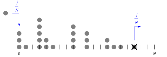
Figure 1: Current reservoirs: particles are injected at the origin at rate $j/N$ and also the rightmost particle is removed with the same rate (two independent clocks are used).

It is worth observing that the replacement of Brownian particles of Chapter 11 with continuous time random walkers allows us to interpret the system as a queuing model with a spatial structure [1, 42]. Namely, customers enter the queue at the origin following a Poisson process, stay in the queue by changing randomly their position and leave the queue when they reach the rightmost site (being served at the event time of another Poisson process). The load of the queue at any given time is thus given by the total particle number, whereas the waiting time before being served is related to the location of the rightmost occupied site.

37 Definition of the model

We consider a Markov process $\{\xi_{t},t\geq 0\}$ on the space $\Omega$ of particles configurations $\xi=(\xi(x))_{x\in[0,N]}$, the component $\xi(x)\in\mathbb{N}$ is interpreted as the number of particles at site $x$. The generator $L$ of the process, working on functions $f:\Omega\to\mathbb{R}$, is the sum of three contributions

$$L=L^{0}+L^{in}+L^{out}\;.$$ (37.1)

The first term $L^{0}$ is the generator of the independent random walks process

$$L^{0}f(\xi)=\frac{1}{2}\sum_{x=0}^{N-1}L^{0}_{x,x+1}f(\xi).$$ (37.2)

$$L^{0}_{x,x+1}f(\xi)=\xi(x)\left(f(\xi^{x,x+1})-f(\xi)\right)+\xi(x+1)\left(f(\xi^{x+1,x})-f(\xi)\right)$$ (37.3)

where $\xi^{x,y}$ denotes the configuration obtained from $\xi$ by removing one particle from site $x$ and putting it at site $y$, i.e.,

$$\xi^{x,y}(z)=\left\{\begin{array}[]{ll}\xi(z)&\text{if }z\neq x,y,\\ \xi(z)-1&\text{if }z=x,\\ \xi(z)+1&\text{if }z=y.\end{array}\right.$$

$L^{0}$ describes independent symmetric random walks which jump with equal probability after an exponential time of mean 1 to the nearest neighbour sites, the jumps leading outside $[0,N]$ being suppressed (reflecting boundary conditions).

The term $L^{in}$ in (37.1) is given by

$$L^{in}f(\xi)=\frac{j}{N}\left(f(\xi^{+})-f(\xi)\right),\quad\xi^{+}(x)=\xi(x)+\delta_{x,0}\;,$$ (37.4)

where $\delta_{x,y}$ denotes the Kronecker delta. For $j>0$, it describes the action of throwing into the system new particles at rate $\frac{j}{N}$, which then land at site 0. Instead $L^{out}$ removes particles and is defined as

$$L^{out}f(\xi)=\frac{j}{N}\left(f(\xi^{-})-f(\xi)\right),\quad\xi^{-}(x)=\xi(x)-\delta_{x,\bar{R}_{\xi}}$$ (37.5)

where

$$\text{ $\bar{R}_{\xi}$ is such that:}\;\;\;\begin{cases}\xi(y)>0&\text{for $y=\bar{R}_{\xi}$}\\ \xi(y)=0&\text{for $y>\bar{R}_{\xi}$}\;.\end{cases}$$ (37.6)

We also impose $L^{in}f(\xi)=0$ if $\bar{R}_{\xi}$ does not exist, i.e. if $\xi\equiv 0$ is the empty configuration.

38 Hydrodynamic limit

The paper [6] proves the existence of the hydrodynamic limit for independent random walkers with current reservoirs on a finite macroscopic volume, i.e. the existence under diffusive space-time scaling of a well-defined function $\rho(r,t)$ describing the evolution of an initial profile $\rho_{\rm init}(r)$. In addition, in [6] it is also proved that $\rho(r,t)$ is the unique separating element of suitably defined barriers.

In this section we recall the main results of [6]. While we refer to the original paper for the proofs, we provide here the main ideas that are used in the proofs. We shall denote by $P^{(N)}_{\xi}$ the law of the process $\{\xi_{t},t\geq 0\}$ in the interval $[0,N]$ with generator $L$ given in (37.1) and started at time 0 from a configuration $\xi$. We consider initial macroscopic profiles $\rho_{\rm init}(r)$ that, similarly to part I, belong to the set

$$\hat{\mathcal{U}}:=\left\{u\in L^{\infty}([0,1],\mathbb{R}_{+})\cap L^{1}([0,1],\mathbb{R}_{+}):\int_{0}^{1}u(r)dr>0\right\}.$$

The configuration $\xi$ from which the process is started must approximate the initial macroscopic profile in the sense of local averages. That is, the following assumptions are made on the initial particle configuration. Fix $0<a,b<1$ and denote denote by $\ell$ the integer part of $N^{b}$. Then we assume that for any $N$ the initial configuration $\xi$ verifies

$$\max_{x\in[0,N-\ell+1]}\Big{|}\frac{1}{\ell}\sum_{y=x}^{x+\ell-1}\xi(y)-\frac{N}{\ell}\Big{(}\int_{x/N}^{x/N+\ell/N}\rho_{\rm init}(r)dr\Big{)}\Big{|}\leq\frac{1}{N^{a}}$$ (38.7)

where $\rho_{\rm init}\in\mathcal{U}$. Moreover, defining the edge of $\rho_{\rm init}$ as

$$R(\rho_{\rm init})=\inf\{r\in[0,1]:\int_{r}^{1}\rho_{\rm init}(r^{\prime})dr^{\prime}=0\}$$ (38.8)

we also suppose that

$$\Big{|}\frac{\bar{R}_{\xi}}{N}-R(\rho_{\rm init})\Big{|}\leq\frac{1}{N^{a}}$$ (38.9)

with $\bar{R}_{\xi}$ the position of the rightmost particle, see (37.6).

The first result in [6] is the following:

Theorem 38.1 (Existence of hydrodynamic limit, [6]).

Let $\rho_{\rm init}\in\hat{\mathcal{U}}$ and $\xi$ an approximation in the sense described above. Then there exists a non-negative, continuous function $\rho(r,t)$ defined on $[0,1]\times\mathbb{R}_{+}$ such that for any $t>0$ and $\zeta>0$,

$$\lim_{N\to\infty}P^{(N)}_{\xi}\Big{[}\max_{x\in[0,N]}\Big{|}\frac{1}{N}\sum_{y=x}^{N}\xi_{N^{2}t}(y)-\int_{x/N}^{1}\rho(r^{\prime},t)dr^{\prime}\Big{|}\leq\zeta\Big{]}=1$$ (38.10)

and such that for any $r\in[0,1]$,

$$\lim_{t\to 0}\int_{r}^{1}\rho(r^{\prime},t)dr^{\prime}=\int_{r}^{1}\rho_{\rm init}(r^{\prime})dr^{\prime}.$$ (38.11)

It is easy to see that the above convergence also implies weak convergence of the density field against smooth test functions $\phi$, i.e. for all $\zeta>0$,

$$\lim_{N\to\infty}P^{(N)}_{\xi}\left[\Big{|}\frac{1}{N}\sum_{x=0}^{N}\phi\left(\frac{x}{N}\right)\xi_{N^{2}t}(x)-\int_{0}^{1}\phi(r)\rho(r,t)dr\Big{|}\leq\zeta\right]=1\;.$$

The proof of Theorem 38.1 (see Figure 2 for a pictorial representation) follows closely the path used to prove the hydrodynamic limit of particle basic problem, Theorem 1. However, in the present setting there are additional difficulties due to the fact that one needs also to consider a diffusive scaling for the microscopic dynamics. We recall the main steps below, commenting on the main differences.

1. The key idea is to define stochastic barriers. These processes, called $\{\xi^{(\delta,-)}_{t},t\geq 0\}$ and $\{\xi^{(\delta,+)}_{t},t\geq 0\}$, satisfy inequalities with respect to the partial order induced by mass transport and they provide lower and upper bounds for the original process.

2. The proof proceeds by considering discrete time intervals of width $\delta N^{2}$. The stochastic barriers $\{\xi^{(\delta,\pm)}_{k\delta N^{2}},k\in\mathbb{N}\}$ converge weakly as $N\to\infty$ to macroscopic objects given, respectively, by the lower barrier $\{\hat{S}_{k\delta}^{(\delta,-)},k\in\mathbb{N}\}$ and the upper barrier $\{\hat{S}_{k\delta}^{(\delta,+)},k\in\mathbb{N}\}$. These barriers are defined similarly to those of part I, however they are slightly different (see below).

3. The proof is concluded by observing that in the limit $\delta\to 0$ the upper and lower barriers converge to the same limit given by the barriers separating element. Thus also the process $\{\xi_{t},t\geq 0\}$, that is squeezed between the two stochastic barriers, converges to such limiting object.

$$\begin{array}[]{lllllc}\xi^{(\delta,-)}_{kN^{2}\delta}&\preccurlyeq&\xi_{kN^{2}\delta}&\preccurlyeq&\xi^{(\delta,+)}_{kN^{2}\delta}&\\ \\ \Bigg{\downarrow}&&\Bigg{\downarrow}&&\Bigg{\downarrow}&\quad\text{as }\quad N\to\infty\\ \\ \hat{S}^{(\delta,-)}_{k\delta}&\preccurlyeq&\hat{S}_{k\delta}&\preccurlyeq&\hat{S}^{(\delta,+)}_{k\delta}&\quad$$\end{array}$$

Figure 2: Scheme of the proof of existence and characterization of the hydrodynamic limit.

The main difference between the barriers $\hat{S}^{\delta,\pm}_{k\delta}$ considered in [6] and the barriers $S^{\delta,\pm}_{k\delta}$ defined in part I are the following:

• In the definition of the free evolution operator the finite volume setting of [6] required to consider the Green function for the heat equation in $[0,1]$ with Neumann boundary conditions:

  $$\hat{G}_{t}^{\rm neum}(r,r^{\prime})=\sum_{k\in\mathbb{Z}}G_{t}(r,r^{\prime}_{k})$$ (38.12)

  $r^{\prime}_{k}$ being the images of $r^{\prime}$ under repeated reflections of the interval $[0,1]$ to its right and left, $G_{t}(r^{\prime},r)$ as in (5.3).

• Furthermore, in the definition of the barriers $\hat{S}^{\delta,\pm}_{k\delta}$ the injection of mass occured at the discrete times. Namely, the free evolution operator was defined as

  $$\hat{T}_{\delta}u(r)=\hat{G}_{t}^{\rm neum}*u(r)$$ (38.13)

  and the cut operator was defined as

  $$\hat{C}_{\delta}u(r)={C}_{\delta}u(r)+j\delta D_{0}$$ (38.14)

  where ${C}_{\delta}$ is the same as Definition 7 and $D_{0}$ denotes the Dirac delta at zero.

Despite these differences, the same analysis of part I could be carried out. In particular the existence of a unique separating element of the barriers could be proved. As a consequence the second result in [6] was the following.

Theorem 38.2 (Characterisation of hydrodynamic limit, [6]).

Let $\rho_{\rm init}\in\mathcal{U}$, then the hydrodynamic limit $\rho(r,t)$ of Theorem 38.1 is the unique separating element of barriers $\hat{S}_{n\delta}^{\delta,\pm}(\rho_{\rm init})$, i.e.,

$$\rho(r,t)=(\hat{S}_{t}\rho_{\text{init}})(r)\;.$$

Remark 38.3.

By the same arguments of part I, we argue that the hydrodynamic limit $\rho(r,t)$ is given by the solution of the FBP associated to the basic model on the domain $[0,1]$. This would essentially be the “restriction” of the basic FBP of part I (which was defined on the whole half-line $\mathbb{R}_{+}$) with the additional constraint that the edge is bounded, i.e. $X_{t}\leq 1$.

Chapter 14 Beyond diffusive scaling

In this chapter we analyze the consequences of having two independent Poisson process for the injection and removal of mass. We use again the model introduced in [6], for which we describe the super-hydrodynamic limit.

39 Introduction

As already remarked in Section 2, there exist stationary classical solutions of the basic FBP on $\mathbb{R}_{+}$. Furthermore, we argued at the end of the previous chapter that the hydrodynamic limit $\rho(r,t)=\hat{S}_{t}\rho_{\rm init}(r)$ of interacting random walkers with current reservoirs is provided by the solution of the basic FBP restricted to the interval $[0,1]$. It is natural then to conjecture that $\rho(r,t)$ converges as $t\to\infty$ to the stationary solutions of the basic FBP on the interval $[0,1]$. However the stationary classical solutions of the basic FBP is not unique, there exists an entire manifold of stationary linear profiles labeled by the mass $M$. As a result, the following questions naturally arise.

• What is the basin of attraction (i.e. the set of initial conditions that will be attracted to a given stationary solution in the course of time)?

• Given the existence of infinitely many stationary linear profiles of the FBP, which one will be selected by the microscopic dynamics?

In this chapter we shall discuss these questions, following the results obtained in [7]. We start by describing in section 40 the stationary profiles of the basic FBP on the interval $[0,1]$ and then we describe their basin of attraction. The second question leads to the identification of a multi-scale phenomenon whose origin is explained in section 41 and whose formulation is given in section 42.

40 Stationary density profiles

The stationary solutions of the basic FBP restricted to the interval $[0,1]$ are similar to those of the basic FBP on $\mathbb{R}_{+}$ already described in Section 2. The difference is that, due to the finite volume, now we need to consider the case of linear profiles truncated at $r=1$, i.e. trapezium-shaped profiles. It is immediate to verify that they are given by

$$\rho_{\rm stat}^{(M)}(r)=\begin{cases}(-2jr+2\sqrt{Mj})\mathbf{1}_{0\leq r\leq\sqrt{M/j}}&\qquad\text{if }M\leq j,\\ (-2jr+M+j)\mathbf{1}_{0\leq r\leq 1}&\qquad\text{if }M>j\;.\end{cases}$$ (40.1)

As in Section 2 they are labeled by the value of the total mass M via the relation

$$\int_{0}^{1}\rho_{\rm stat}^{(M)}(r)dr=M.$$ (40.2)

For later convenience we also define $\rho_{\rm stat}^{(0)}\equiv 0$.

The following result is proved in [7]. It identifies the basin of attraction of the linear profiles through the analysis of their stability.

Theorem 40.1 (Convergence to the stationary profiles, [7]).

For $r\in[0,1]$, $t>0$ let $\rho(r,t)=\hat{S}_{t}\rho_{\rm init}(r)$, be the hydrodynamic limit of the process defined in section 37 with initial configuration $\xi$ approximating the initial profile $\rho_{\rm init}$ such that $\int_{0}^{1}\rho_{\rm init}(r)dr=M$. Then

$$\lim_{t\to\infty}\sup_{r\in[0,1]}\Big{|}\int_{r}^{1}\rho(r^{\prime},t)dr^{\prime}-\int_{r}^{1}\rho_{\rm stat}^{(M)}(r^{\prime})dr^{\prime}\Big{|}=0\;.$$ (40.3)

41 The law of the total mass

For the system of independent random walkers with current reservoirs defined in section 37, we consider the process $\{|\xi_{t}|,t\geq 0\}$ yielding the particles’ number at time $t$, i.e.,

$$|\xi_{t}|=\sum_{x=0}^{N}\xi_{t}(x)\;.$$ (41.4)

The next theorem shows that this process is very simple, despite the complexity of the full process $\{\xi_{t},t\geq 0\}$.

Theorem 41.1 (Number of particles).

The process $\{|\xi_{t}|,t\geq 0\}$ has the law of a simple symmetric random walk on $\mathbb{N}$ which jumps with equal probability by $\pm 1$ after an exponential time of parameter $\frac{2j}{N}$, the jumps leading to $-1$ being suppressed.

Proof. From the generator (37.1) we deduce the generator of the particle’s number process $\{|\xi_{t}|,t\geq 0\}$ :

$${\cal L}f(n)=\frac{j}{N}\Big{\{}\big{(}f(n+1)-f(n)\big{)}+(1-\delta_{|\xi|,0})\big{(}f(n-1)-f(n)\big{)}\Big{\}}$$ (41.5)

where $f$ denotes a bounded function $f:\mathbb{N}\to\mathbb{R}$. This coincides with the generator of the simple symmetric random walk on $\mathbb{N}$ that jumps at rate $\frac{j}{N}$ and is reflected at the origin. This uniquely characterize the law of $\{|\xi_{t}|,t\geq 0\}$. ∎

An immediate consequence of the previous Theorem is the following

Corollary 41.2 (Scaling limit).

Let $\rho_{\rm init}\in\hat{\mathcal{U}}$ and $\xi\in\Omega$ such that

$$M:=\lim_{N\to\infty}\frac{|\xi|}{N}=\int_{0}^{1}\rho_{\rm{init}}(r)dr.$$ (41.6)

Let $\{\xi_{t},t\geq 0\}$ be the processis initialized from $\xi$, then the following scaling limits hold:

$$\frac{|\xi_{N^{2}t}|}{N}\to M\qquad\qquad\text{as}\quad N\to\infty,$$ (41.7)

$$\frac{|\xi_{N^{3}t}|}{N}\to B_{jt}\qquad\qquad\text{as}\quad N\to\infty$$ (41.8)

where the converge is in law and $\{B_{t},{t\geq 0}\}$ denotes the Brownian motion on $\mathbb{R}_{+}$ with reflections at the origin which starts from $B_{0}=M$.

42 Super-hydrodynamic limit

Hydrodynamics describes the behavior of the system on times $N^{2}t$ in the limit when $N\to\infty$. Hydrodynamics predicts convergence to equilibrium as in Theorem 40.1. As a consequence of (40.3) we have that for any $\zeta>0$,

$$\lim_{t\to\infty}\lim_{N\to\infty}P_{\xi}^{(N)}\Big{[}\max_{x\in[0,N]}\;\Big{|}\frac{1}{N}\sum_{y=x}^{N}\xi_{N^{2}t}(y)-\int_{x/N}^{1}\rho_{\rm{stat}}^{(M)}(r^{\prime})dr^{\prime}\Big{|}{\geq\zeta\Big{]}=0}$$ (42.9)

where $M=\int_{0}^{1}\rho_{\rm init}(r)dr$. (42.9) shows convergence of the macroscopic density field to the invariant profiles. Thus, on the hydrodynamic time-scale, the profile that is selected by the system is dictated by the total mass, which is a conserved quantity on the time scale $N^{2}t$.

However, if one inverts the order of the two limits in (42.9) then a different result would be obtained. Indeed, due to the result in the previous section, on a longer time scale over which fluctuations of the total mass are allowed, there is not anymore a privileged profile. The investigation of the long time behavior requires the study of the process at times ${N^{2}t_{N}}$ where $t_{N}\to\infty$ as $N\to\infty$. If in this limit we obtain something different from (42.9) then we can conclude that there are other significant time-scales beyond the hydrodynamical one. This has been proved in [7], from which we quote the following

Theorem 42.1 (Super-hydrodynamic limit, [7]).

Let $\xi$ be a sequence such that $\frac{|\xi|}{N}\to M>0$ as $N\to\infty$. Let $t_{N}$ be an increasing, divergent sequence, then the process $\xi_{N^{2}t_{N}}$ has two regimes:

• Subcritical. If $Nt_{N}\to 0$, then

  $$\lim_{N\to\infty}P_{\xi}^{(N)}\Big{[}\max_{x\in[0,N]}\;\Big{|}\frac{1}{N}\sum_{y=x}^{N}\xi_{N^{2}t_{N}}(y)-\int_{x/N}^{1}\rho_{\rm{stat}}^{(M)}(r^{\prime})dr^{\prime}\Big{|}{\leq\zeta\Big{]}=1}.$$ (42.10)

• Critical. Let $t_{N}=Nt$ then

  $$\lim_{N\to\infty}P_{\xi}^{(N)}\Big{[}\max_{x\in[0,N]}\;\Big{|}\frac{1}{N}\sum_{y=x}^{N}\xi_{N^{3}t}(y)-\int_{x/N}^{1}\rho_{\rm{stat}}^{(M_{t}^{(N)})}(r^{\prime})dr^{\prime}\Big{|}{\leq\zeta\Big{]}=1}$$ (42.11)

  where $M^{(N)}_{t}:=\frac{|\xi_{N^{3}t}|}{N}$ converges in law as $N\to\infty$ to $B_{jt}$, where $(B_{t})_{t\geq 0}$ is the Brownian motion on $\mathbb{R}_{+}$ with reflections at the origin started from $B_{0}=M$.

We refer to [7] for the proof of the theorem. We conclude this section with the following comment. On a first time scale, i.e. the subcritical regime, the process behaves deterministically and it is attracted to the invariant linear profile with mass M (the mass at time zero). However on longer times of the order $N^{3}t$ it starts moving stochastically on the manifold of the linear profiles where it performs a Brownian motion (with reflection at 0 since the mass can not become negative). Thus a random behavior arises again on the super-hydrodynamic time scale.

Chapter 15 Other models

In this chapter we discuss very briefly other models which have several features in common with our basic model. The interaction at the particle level has in fact in these models a topological nature as the rightmost and/or the leftmost particles act differently from the others. At the macroscopic level this is reflected by a PDE with a free boundary where the evolution of the edges has to be determined via the outgoing or incoming flux. The models we present have these features and they can be studied (or have been studied) using barrier inequalities as in Part I. The strategy is thus the same but the mathematical problems in its implementation can be quite different.

The models we are going to present have a natural biological motivation. Particles represent cells, particles positions the states of the cells. The natural order in $\mathbb{R}$ is used to express the fitness of a cell state, for instance the rightmost cell could be the best fitted in the whole population (of course same analysis would apply when we exchange right and left). Cells are not clever, they do not know what is best for them and mutate by exploring all possible nearby states, this is modeled by the cells performing independent Brownian motions. Cells also duplicate independently of each other this is modeled by adding a new particle say at rate 1 in the same state of the duplicating cell (or in one nearby). The body which contains the cells cannot support any number of cells, we suppose that a saturation point has been reached for which the number of cells, say $N$, does not change in time. This means that when a cell duplicates then another cell must be removed from the system. Here nature imposes its Darwinian law for which the cell removed is the less fitted, the weakest one. A model with these features has been introduced by Brunet-Derrida and studied by several authors as we will discuss in the sequel.

The question we address and partially answer are: (1) hydrodynamic limit, i.e. the FBP associated to the particle model; (2) validity of barrier inequalities; (3) existence and features of stationary states (or traveling waves).

43 Cells evolution in an active environment

Here we consider a variant of the Brunet-Derrida model described above where (1) cells are Brownian particles in $\mathbb{R}_{+}$ (with reflections at the origin), the cell states (as in the Brunet-Derrida case) are the positions of the particles, but here their fitness decreases when moving to the right, so that $0$ is the best fitted state; (2) it is the environment which creates new cells so that we have an a-priori given probability density $f(r)$, $r\in\mathbb{R}_{+}$, with compact support and the state of a new born cell is randomly distributed with law $f(r)dr$; (3) to preserve, as in the Brunet-Derrida model, the total number $N$ of cells when a new cell is created the rightmost cell (i.e. the weakest, less fitted) is removed; (4) the rate at which a new cell is added is set equal to $N$ (which corresponds to the rate in Brunet-Derrida because in that case each particle duplicates at rate 1 so that the intensity for a new particle to appear is $N$).

If $f(r)dr$ is replaced by a delta function at 0 then this becomes the basic model we have studied in Part I (with the parameter $j$ set equal to 1). If instead

$$f(r)dr=\frac{1}{N}\sum_{i=1}^{N}\delta_{x_{i}}(dr)$$

where $\underline{x}=(x_{1},..,x_{N})$ is the actual configuration of the cells, then this would be the Brunet-Derrida model (in $\mathbb{R}_{+}$). In the diffuse case (where $f(r)$ is a fixed true function) it may happen that the state of a new born cell is to the right of all the others. In such a case the new cell is also the rightmost one and it is thus removed right away. This leads to the conjecture that the hydrodynamic limit for this system is ruled by the following FBP:

$$\frac{\partial\rho}{\partial t}=\frac{1}{2}\frac{\partial^{2}\rho}{\partial r^{2}}+f,\quad r\in(0,X_{t})$$ (43.1)

with an initial datum $\rho_{0}$, Neumann boundary condition at 0

$$\frac{\partial\rho(r,t)}{\partial r}\Big{|}_{r=0}=0$$ (43.2)

while, at the edge $X_{t}$, $\rho(X_{t},t)=0$ and

$$-\frac{1}{2}\frac{\partial\rho(r,t)}{\partial r}\Big{|}_{r=X_{t}}=\phi(X_{t}),\;\phi(x):=\int_{0}^{x}f(r).$$ (43.3)

Namely denoting as in Chapter 11 by $\pi_{t}^{(N)}(dr)$ the empirical particles density we conjecture that for any $\epsilon>0$:

$$\lim_{N\to\infty}P^{(N)}\Big{[}\sup_{r\geq 0}\Big{|}\int_{r}^{\infty}\pi_{t}^{(N)}(dr^{\prime})-\int_{r}^{\infty}\rho(r^{\prime},t)dr^{\prime}\Big{|}>\epsilon\Big{]}=0$$ (43.4)

where $\rho(r,t)$ is the classical or relaxed solution of (43.1)–(43.2)–(43.3)

The proofs of Part I should extend to this case at least when the edge (of the approximating barriers) is to the right of the support of $f$, the analysis of the general case may be more delicate.

Stationary profiles are analogous to those of (2.1) (to which they reduce when $f$ is a delta)

$$\rho^{(st)}(r|M)=a(M)-2j\int_{0}^{r}\phi(r^{\prime})dr^{\prime}\mathbf{1}_{a(M)-2j\int_{0}^{r}\phi(r^{\prime})dr^{\prime}\geq 0},\quad\int\rho^{(st)}(r|M)=M$$ (43.5)

and are parameterized by the mass $M$ which is conserved.

44 The Brunet-Derrida evolution-selection mechanism

The Brunet-Derrida model is the one described in the beginning of this chapter. Namely the cell evolution is described by independent Brownian motions on $\mathbb{R}$, each cell duplicates independently of the others at rate 1 creating a new Brownian particle in its same state, simultaneously the rightmost particle is deleted. The conjectured hydrodynamic limit in this system is

$$\frac{\partial\rho}{\partial t}=\frac{1}{2}\frac{\partial^{2}\rho}{\partial r^{2}}+\rho,\quad{\rm in}\;\;[L_{t},+\infty)$$ (44.1)

with initial state $\rho_{0}(r)$ and boundary conditions at the free boundary $L_{t}$ given by $\rho(L_{t},t)=0$ and

$$\frac{\partial\rho(r,t)}{\partial r}\Big{|}_{r=0}=0;\quad\frac{1}{2}\frac{\partial\rho(r,t)}{\partial r}\Big{|}_{r=L_{t}}=M,\;M:=\int_{0}^{X_{t}}\rho(r,t).$$ (44.2)

There is a paper in preparation by A. De Masi, P. Ferrari, E. Presutti and N. Soprano-Loto which goes in this direction, namely that the evolution of the cells in this model is described in the hydrodynamic limit by the above FBP, the analysis follows the strategy described in Part I.

On the whole line there are no longer stationary solutions but there are traveling waves. One can in fact check that $\rho(r,t)=\rho^{(tw)}(r-Vt)$ solves (44.1)–(44.2) where

$$\rho^{(tw)}(r)=MV^{2}re^{-Vr},\quad V^{2}=2.$$ (44.3)

This is not the only traveling wave (with mass $M$) but it is the one with the minimal velocity. We refer the reader for more details and for related models to the review article [31].

An interesting (perhaps basic) question is whether there is a stationary, or in this case traveling, measure for the particle system when $N$ is fixed and if its velocity (in the case of traveling waves) is close to the one found by solving the analogous problem for the hydrodynamic equation. This is not at all obvious as the latter describe the behavior of the system when time is fixed and the number $N$ of particles goes to infinity while we want first to take $t\to\infty$ and then $N\to\infty$. The analysis of the motion of the system at finite $N$ has been investigated thoroughly by by P. Maillard, [37], who has studied the system at times $\log^{3}N$ determining the law of the fluctuations of the edge.

45 The Durrett and Remenik model

Durrett and Remenik, [18], have studied a variant of the Brunet-Derrida model where cells do not change their states, but they duplicate in a non-local way. Namely each cell (independently of the others) creates at rate 1 a new cell in a state $r\in\mathbb{R}$ which is randomly chosen with probability $\kappa(r-r^{\prime})dr$, if $r^{\prime}$ is the state of the generating cell; $\kappa$ is a smooth probability kernel. As in Brunet-Derrida simultaneously to the creation of the new cell the leftmost one is erased.

In [18] it is shown that for suitable initial data there is a hydrodynamic limit described by the equation

$$\frac{\partial}{\partial t}\rho(r,t)=\int\kappa(r^{\prime}-r)\rho(r^{\prime},t)dr^{\prime}$$ (45.1)

with $\rho(r,0)=\rho_{0}(r)$, $\int\rho_{0}=:M$, and boundary conditions at the left edge $L_{t}$:

$$\rho(L_{t}^{-},t)=0,\quad\int_{L_{t}}^{\infty}\rho(r,t)=M.$$ (45.2)

The proof uses barriers in a way similar to that in Part I and traveling fronts are determined.

46 Models with two species

A natural extension of the previous models is when there are two species of cells, say $R$ and $B$ (red and blue). The cells live both in $\mathbb{R}$ whose points give their degree of fitness (like in the Brunet-Derrida model). However for the red particles fitness increases to the right while for the blue to the left. We suppose that there are $N$ red and $N$ blue particles, their number being conserved. As in the previous models the cells move like independent Brownian motions however at rate $N$ the weakest red (i.e. the leftmost red particle) becomes blue and the weakest blue (i.e. the rightmost blue particle) becomes red.

In [12] for a similar model it has been proved that in the hydrodynamic limit the system is described by the following FBP:

$$\hskip-14.22636ptu_{t}=\frac{1}{2}u_{rr}+j\,\delta_{V_{t}},\;r<U_{t};\;u(r,0)=u(r),\;u(U_{t},t)=0,\;-\frac{1}{2}u_{r}(U^{-}_{t},t)=j,$$

(46.1)

$$\hskip-14.22636ptv_{t}=\frac{1}{2}v_{rr}+j\,\delta_{U_{t}},\;r>V_{t};\;v(r,0)=v(r),\;v(V_{t},t)=0,\;-\frac{1}{2}v_{r}(V^{+}_{t},t)=-j,$$

(under the assumption that this has a classical solution). (46.1) is a system of two free boundary equations as the domains $(-\infty,U_{t})$ where $u(r,t)$ is defined and $(V_{t},\infty)$ where $v(r,t)$ is defined are also unknowns to be determined.

So far we have considered models where the particles move independently, Brownian motions or independent random walks. In the next model there is an interaction between particles. This is still a two species model but particles are on $\mathbb{Z}$ with a constraint: at each site there is one particle either red or blue. Their motion is defined by the “stirring process”, namely at rate $1/2$ each pair $x,x+1$ of successive points of $\mathbb{Z}$ exchange their content independently of all the other pairs, so that if at $x,x+1$ we had $R,B$ after the stirring we have $B,R$. If instead we had $B,B$ or $R,R$ the stirring does not produce any effect. Thus the particles are no longer independent, when a particle jumps from $x$ to $x+1$ it forces the opposite jump of another particle.

Allowed configurations are those where there is a rightmost blue and a leftmost red particle. We may describe the system by giving the positions of only the blue particles (because if at a site there is not a blue particle then there is a red particle), we thus introduce a variable $\eta(x,t)$ equal to 1 when at $x,t$ there is a blue particle and equal to 0 otherwise. Allowed configurations are therefore those where $\eta(x)=1$ definitively as $x\to-\infty$ and $\eta(x)=0$ as $x\to+\infty$. The evolution is determined by the stirring process described earlier and by a “selection mechanism” which here is defined by saying that at rate $\epsilon$ the leftmost $0$ becomes 1 and the rightmost $1$ becomes a 0. In [13] it is proved that under suitable assumptions on the initial distribution of particles, when space is scaled as $\epsilon^{-1}$ and time as $\epsilon^{-2}$ the empirical density of 1’s converges to a limit which is conjectured to satisfy the FBP:

$$\frac{\partial\rho}{\partial t}=\frac{1}{2}\frac{\partial^{2}\rho}{\partial r^{2}},\quad r\in(L_{t},R_{t}),$$ (46.2)

$$L_{0},R_{0},\rho(r,0)\;\text{given}$$

$$\rho(L_{t},t)=1,\;\;\rho(R_{t},t)=0;\quad\frac{\partial\rho}{\partial r}(L_{t},t)=\frac{\partial\rho}{\partial r}(R_{t},t)=-2j.$$

This is proved using the same strategy as in Part I, actually [13] is the paper where such a strategy has been introduced. Thus there exist lower and upper barriers which squeeze in between the actual evolving configuration as described in Part I. To prove convergence to (46.2) we would need to reproduce the analysis of Chapter 10.

47 Interface models

The particle system described at the end of the previous section has also an interpretation in terms of moving interfaces. The interface is a graph in $\mathbb{Z}^{2}$ determined by the particles configuration: if $(x,y)$ belongs to the interface and $\eta(x)=1$ then $(x+1,y-1)$ also belongs to the interface, while if $\eta(x)=0$ then the next point of the interface is $(x+1,y+1)$. The correspondence is one to one if we fix for instance the height of the interface at $0$. The evolution of the particles determines the motion of the interface.

[33] studies the stochastic evolution of interfaces over a “sticky substrate”, we refer to [33] for the exact definition of the model. The paper contains a full proof of the hydrodynamic limit for this system, the limit hydrodynamic equation written in terms of the underlying particle system is the FBP

$$\frac{\partial}{\partial t}\rho(r,t)=\frac{1}{2}\frac{\partial^{2}}{\partial r^{2}}\rho(r,t),\quad r\in(L_{t},R_{t})$$ (47.1)

with given initial condition $\rho(r,0)=\rho_{0}(r)$ and boundary conditions at the free boundaries:

$$\frac{\partial}{\partial r}\rho(r,t)\Big{|}_{r=R_{t}}=-\frac{1}{2}\frac{\partial}{\partial r}\rho(r,t)\Big{|}_{r=L_{t}}=\frac{1}{2}.$$ (47.2)

Global existence of the classical solution of (47.1) (till extinction) is also proved in [33].

(47.2) appears also in the analysis of propagation of fire, see for instance Caffarelli-Vazquez, [4]. In the $d\geq 1$ setup the FBP in its classical formulation is:

$$\frac{\partial}{\partial t}\rho=\frac{1}{2}\Delta\rho,\quad r\in\Omega_{t}$$ (47.3)

with boundary conditions $\rho=0$ and $\nabla\rho\cdot n=-\frac{1}{2}$ on $\partial\Omega_{t}$, ($n$ the outward normal unit vector to $\Omega_{t}$ at the boundary $\partial\Omega_{t}$). We refer to the literature for an analysis of this FBP and of other related models.

References

• [1] J. Anselmi, B. D’Auria, N. Walton, Closed queueing networks under congestion: non-bottleneck independence and bottleneck convergence. Mathematics of Operations Research 38, 469–491 (2013).
• [2] E. Brunet, B. Derrida, Shift in the velocity of a front due to a cutoff. Physical Review E 56, 2597–2604 (1997).
• [3] E. Brunet, B. Derrida, Effect of macroscopic noise on front propagation. Journal of Statistical Physics 103, 269–282 (2001).
• [4] L. A. Caffarelli, J. L. Vazquez, A free boundary problem for the heat equation arising in flame propagation. Transactions American Mathematical Society 347, 411–441 (1995).
• [5] J. R. Cannon, The one-dimensional heat equation. Encyclopedia of mathematics and its applications 23, Addison-Wesley Publishing Company (1984).
• [6] G. Carinci, A. De Masi, C. Giardinà, E. Presutti, Hydrodynamic limit in a particle system with topological interactions. Arabian Journal of Mathematics 3, 381–417 (2014).
• [7] G. Carinci, A. De Masi, C. Giardinà, E. Presutti, Super-hydrodynamic limit in interacting particle system. Journal of Statistical Physics 155, 867–887 (2014).
• [8] L. Chayes, I. Kim, The supercooled Stefan problem in one dimension. Communication on Pure and Applied Analysis 11, 845–859 (2012).
• [9] L. Chayes, G. Swindle, Hydrodynamic limits for one-dimensional particle systems with moving boundaries. Annals of Probability 24, 559–598 (1996).
• [10] J. Crank and R. S. Gupta, A method for solving moving boundary problems in heat-flow using cubic splines or polynomials. Journal of the Institute of Mathematics and its Applications 10, 296–304 (1972).
• [11] E. De Giorgi, New ideas in calculus of variations and geometric measure theory. Proceedings of the Conference Motion by Mean Curvature and Related Topics, held in Trento, 1992, pp. 63–69, Walter de Gruyter, Berlin (1994).
• [12] A. De Masi, P.A. Ferrari, Separation versus diffusion in a two species system. Brazilian Journal of Probability and Statistics 29, 387–412 (2015).
• [13] A. De Masi, P.A. Ferrari, E. Presutti, Symmetric simple exclusion process with free boundaries. Probability Theory and Related fields 161, 155–193 (2015).
• [14] A. De Masi, E. Presutti, D. Tsagkarogiannis, M.E. Vares, Current reservoirs in the simple exclusion process. Journal of Statistical Physics 144, 1151–1170 (2011).
• [15] A. De Masi, E. Presutti, D. Tsagkarogiannis, M.E. Vares, Exponential rate of convergence in current reservoirs. Bernoulli 21(3), 1844–1854 (2015).
• [16] A. De Masi, E. Presutti, D. Tsagkarogiannis, M.E. Vares, Truncated correlations in the stirring process with births and deaths. Electronical Journal of Probability 17, 1–35, (2012).
• [17] A. De Masi, E. Presutti, D. Tsagkarogiannis. Fourier law, phase transitions and the stationary Stefan problem. Archive for Rational Mechanics and Analysis 201, 681–725 (2011).
• [18] R. Durrett, D. Remenik, Brunet-Derrida particle systems, free boundary problems and Wiener-Hopf equations. Annals of Probability 39, 2043–2078 (2011).
• [19] J. Douglas, A uniqueness theorem for the solution of a Stefan problem. Proceedings of the American Mathematical Society 8(2), 402–408 (1957).
• [20] A. Fasano, Mathematical models of some diffusive processes with free boundaries. SIMAI e-Lecture Notes (2008).
• [21] A. Fasano and M. Primicerio, General free boundary problems for the heat equation, I. Journal of Math Analysis and Applications 57, 694–723 (1977).
• [22] A. Fasano and M. Primicerio, General free boundary problems for the heat equation, II. Journal of Math Analysis and Applications 58, 202–231 (1977).
• [23] A. Fasano and M. Primicerio, General free boundary problems for the heat equation, III. Journal of Math Analysis and Applications 59, 1–14 (1977).
• [24] A. Fasano and M. Primicerio, Free boundary problems for nonlinear parabolic equations with nonlinear free boundary conditions. Journal of Math Analysis and Applications 72, 247–273 (1979).
• [25] A. Fasano, M. Primicerio, S.D. Howison and J.R. Ockendon, Some remarks on the regularization of supercooled one-phase Stefan problems in one dimension. Quarterly of Applied Mathematics 48 153–168 (1990).
• [26] A. Fasano, M. Primicerio, S.D. Howison and J.R. Ockendon, On the singularities of one-dimensional Stefan problems with supercooling. In Mathematical Models for Phase Change Problems, J.F. Rodrigues, editor. Int. Ser. Numerical Mathematics 88, 215–225 (1989), Birkhauser,
• [27] A. Friedman, Free boundary problems for parabolic equations. Technical Report Report No. 28, Office of Naval Research (1958).
• [28] A. Friedman, Partial Differential Equations of Parabolic Type, Holt, Reinhart, and Winston Inc., New York (1964).
• [29] J.B.J. Fourier, Théorie analytique de la chaleur, Firmin-Didot, Paris (1822).
• [30] J. Gravner, J. Quastel, Internal DLA and the Stefan problem. Annals of Probability 28, 1528–1562 (2000).
• [31] P. Groisman, M Jonckheere, Front propagation and quasi-stationary distributions: the same selection principle?. ArXiv preprint ArXiv:1304.4847 (2013).
• [32] I. C. Kim, A free boundary problem arising in flame propagation. Journal of Differential Equations 191, 470–489, (2003).
• [33] H. Lacoin, The scaling limit of polymer pinning dynamics and a one dimensional Stefan freezing problem. Communications on Mathematical Physics 331, 21–66 (2014).
• [34] C. Landim and G. Valle, A microscopic model for Stefan melting and freezing problem. Annals of Probability 34, 779–803 (2006).
• [35] G.M. Lieberman, Second order parabolic differential equations. World scientific (1996).
• [36] S. Luckhaus, Solutions for the two phase Stefan problem with the Gibbs Thompson law for the melting temperature. European Journal of Applied Mathematics 1, 101–112 (1990).
• [37] P. Maillard, Speed and fluctuations of $N$ particle branching Brownian motion with spatial selection. ArXiv preprint ArXiv:1304.0562 (2013).
• [38] G. Peskir, A. Shiryaev Optimal stopping and Free-boundary problems. Lecture in Mathematics ETH Zürich Birkh user (2006).
• [39] J. R. Ockendon, The role of the Crank-Gupta model in the theory of free and moving boundary problems. Advances in Computational Mathematics 6 281–293 (1996).
• [40] D. Revuz, M. Yor, Continuous martingales and Brownian motion, Vol. 293 of Grundlehren der Mathematischen Wissenschaften. Springer-Verlag, Berlin, third edition, 1999.
• [41] V.A. Roklin, On the fundamental ideas of measure theory. Amer. Math. Soc. Translations Series 1. 10, 1–52 (1962).
• [42] R. Srinivasan, Queues in Series via Interacting Particle. Mathematics of Operations Research 18, 39–50 (1993).
• [43] J. Stefan, Uber die Theorie der Eisbildung. Monatshefte Mat. Phys. 1, 1–6 (1890).
• [44] A. Visintin, Introduction to Stefan-type problems. In: Handbook of Differential Equations: Evolutionary Differential Equations vol. IV (C. Dafermos and M. Pokorny, eds.) North-Holland, Amsterdam, chap. 8, pp. 377–484 (2008).
Conversion to HTML had a Fatal error and exited abruptly. This document may be truncated or damaged.