Stochastic timing in gene expression for simple regulatory strategies

Abstract

Timing is essential for many cellular processes, from cellular responses to external stimuli to the cell cycle and circadian clocks. Many of these processes are based on gene expression. For example, an activated gene may be required to reach in a precise time a threshold level of expression that triggers a specific downstream process. However, gene expression is subject to stochastic fluctuations, naturally inducing an uncertainty in this threshold-crossing time with potential consequences on biological functions and phenotypes. Here, we consider such “timing fluctuations”, and we ask how they can be controlled. Our analytical estimates and simulations show that, for an induced gene, timing variability is minimal if the threshold level of expression is approximately half of the steady-state level. Timing fluctuations can be reduced by increasing the transcription rate, while they are insensitive to the translation rate. In presence of self-regulatory strategies, we show that self-repression reduces timing noise for threshold levels that have to be reached quickly, while self-activation is optimal at long times. These results lay a framework for understanding stochasticity of endogenous systems such as the cell cycle, as well as for the design of synthetic trigger circuits.

I Introduction

Several cellular processes rely on a precise temporal organisation Pedraza2007 ; Yurkovsky2013 . Prominent examples are the controls of the cell cycle and of circadian clocks, where the timing precision can be crucial for the correct cellular physiology Pedraza2007 ; Bean2006 . Similarly, the complex patterns of sequentially ordered biochemical events that are often observed in development and cell-fate decision presumably require a tight control of expression timing Eldar2010 ; Yosef2011 ; Kuchina2011 . Typically, internal signals and environmental cues induce the expression of one or several regulators, which in turn can trigger the appropriate cellular response when their concentration reach a certain threshold level Pedraza2007 ; Singh2014 .

However, a gene may reach a target level of expression with substantial cell-to-cell variability, even in a genetically identical population of cells exposed to the same stimulus. This variability is a necessary consequence of the intrinsically stochastic nature of gene expression Paulsson2004 ; Raj2008 . For genes whose expression has to reach a trigger threshold level, noise in gene expression leads to variability in the time required to reach the target level. This raises the question of what is the extent of this variability and which regulatory strategies can control such fluctuations. Most studies have focused on fluctuations in molecule numbers at equilibrium, while comparatively very few studies have addressed the problem of timing fluctuations theoretically Murugan2011 ; Singh2014 ; Yurkovsky2013 or experimentally Amir2007 ; Pedraza2007 ; Nachman2007 .

Here, we develop analytical estimates and simulations to study the fluctuations in the time necessary to reach a target expression level after gene induction, and we investigate the effect of simple regulatory strategies on these fluctuations. We first consider the case of an unregulated gene whose expression is switched on, and we ask what are the relevent parameters defining the crossing-time fluctuations and how these fluctuations can eventually be reduced by the cell. Second, we investigate the role of simple regulatory strategies in controlling the expression timing fluctuations, focusing on the two circuits of positive and negative transcriptional self-regulation.

Understanding expression timing variability is key to approach basic biological mechanisms at the single-cell level. Isolating the possible regulatory strategies able to control this variability can be useful to decipher the design principles behind regulatory networks associated to cellular timing.

With todays experimental techniques based on fluorescence time-lapse microscopy Young2012 , potentially coupled with microfluidic devices to keep cells in a controlled environment for many generations Bennett2009 ; Long2014 , data on gene expression timing and its fluctuations will be more and more accessible in the next years. Therefore, a parallel theoretical understanding of timing fluctuations is necessary to interpret this upcoming data, to design focused experiments, and eventually to engineer synthetic circuits with specific timing properties.

II MATERIALS AND METHODS

II.1 Background on the “standard model” for gene expression

H

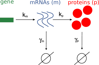
Figure 1: Model of gene expression. A basic description of gene expression includes transcription, translation and molecule degradation. The model described by Eqs. 1 and their stochastic version is based on this scheme.

We employed a standard model of stochastic gene expression Paulsson2005 (Fig. 1) taking into account messenger RNA (mRNA) and protein production and degradation as first-order chemical reactions (with rates $k_{m},k_{p}$ for productions and $\gamma_{m},\gamma_{p}$ for degradations) Paulsson2005 ; Kaern2005 ; BarEven2006 ; Shahrezaei2008 . The rate equations describing the average mRNA and protein dynamics are

$$\frac{d{m(t)}}{{dt}} = k_{m}-\gamma_{m}m(t)$$

$$\frac{d{p(t)}}{{dt}} = k_{p}m(t)-\gamma_{p}p(t).$$ (1)

Since the gene expression process in Fig. 1 does not entail any transcriptional or post-transcriptional regulation we refer to it as “constitutive” expression in the following. However, we are interested in the activation dynamics to evaluate the time (and its fluctuations) necessary to reach a certain level of expression (Fig. 2). Thus, the case of a step induction of transcription will be considered, following e.g. ref. Rosenfeld2002 . The kinetics after a step induction is modeled by the solution of Eqs. 1 with initial conditions $m(0)=0$ and $p(0)=0$

$$p(t) = p_{ss}\left(\frac{\gamma_{p}(1-e^{-\gamma_{m}t})-\gamma_{m}(1-e^{-\gamma_{p}t})}{\gamma_{p}-\gamma_{m}}\right)$$ (2)

$$\simeq p_{ss}(1-e^{-\gamma_{p}t}),$$

where $p_{ss}=k_{p}k_{m}/\gamma_{m}\gamma_{p}$ is the protein steady-state value, and the approximation holds for a protein halflife much longer than the mRNA halflife, i.e., $\eta=\gamma_{p}/\gamma_{m}\ll 1$. Indeed, especially in microorganism such as bacteria and yeast, proteins are typically stable, with a lifetime longer than the cell cycle, while mRNAs have a lifetime of just few minutes Taniguchi2010 ; Shahrezaei2008 , justifying the assumption $\eta\ll 1$ Thattai2001 ; Shahrezaei2008 . Moreover, the loss of highly stable proteins, captured by the rate $\gamma_{p}$, is mainly due to dilution through growth and cell division, so that an effective degradation rate $\gamma_{p}=\mu~{}ln2$ (where the growth rate $\mu$ is the the inverse of the cell doubling time) can be safely assumed in most cases Osella2013 .

The threshold level $\tilde{p}$ of protein expression to be crossed was defined in units of the steady-state value of expression, with the dimensionless parameter $\alpha=\tilde{p}/p_{ss}$ (Fig. 2) . Given the threshold $\alpha$, the corresponding average crossing time can be numerically calculated from Eq.  2, while it takes the simple form $t\simeq-log(1-\alpha)/\gamma_{p}$ for $\eta\ll\ 1$.

The master equation controlling the time evolution of the probability of having $m$ mRNAs and $p$ proteins at time $t$ can be solved analytically for constitutive expression Shahrezaei2008 . Since the mRNA dynamics is described by a birth-death process, the distribution of mRNA numbers is Poisson. By contrast, protein abundance follows a broader distribution, because of the amplification of mRNA fluctuations by protein translation bursts. The model predicts at steady state a negative binomial distribution Shahrezaei2008 , and a gamma distribution in the limit of $p$ continuous Friedman2006 . Fluctuations in protein number can be measured by the Coefficient of Variation (CV) which is the ratio between the standard deviation and the average number of proteins $CV_{p}(t)=\sigma_{p}(t)/\langle p(t)\rangle$. The time evolution of this noise measure has a particularly compact form in the regime of $\eta\ll 1$ Shahrezaei2008 :

$$CV_{p}(t)^{2}=\frac{1}{\langle p(t)\rangle}(1+b+be^{-\gamma_{p}t}),$$ (3)

where $b=k_{p}/\gamma_{m}$ is the burst size, i.e., the average number of proteins produced during a mRNA lifetime, while the dynamics of $\langle p(t)\rangle$ is described by the deterministic equation (Eq. 2). The burst size represents the amplification factor of noise with respect to the Poisson noise of the mRNA. Indeed, the noise expression at steady state $CV_{p}^{2}=\frac{1}{\langle p\rangle_{ss}}(1+b)$ explicitily shows a noise term proportional to $b$ in addition to the Poisson scaling $\sim 1/\langle p\rangle$. A “burst frequency” parameter $a=k_{m}/\gamma_{p}$ can be defined so that the average protein level at steady state is expressed as the product $\langle p\rangle_{ss}=a~{}b$.

Estimate of biologically relevant parameter values

The biologically relevant range of parameters can be extrapolated from large-scale measurements of gene expression at the single cell level. For E. coli in particular, proteins and mRNAs have been measured with single-molecule sensitivity for $\sim 10^{3}$ genes Taniguchi2010 . In this dataset, the average mRNA lifetime is $~{}5$ minutes, which corresponds to a degradation rate of $\gamma_{m}=0.2$. Protein lifetime is often longer then the duration of the cell cycle, which may span from $20$ minutes to several hours in fast-growing bacteria like E. coli. Thus, protein dilution in fast-growth conditions defines the maximum value $\gamma_{p}\simeq 0.03$ min^-1 for effective protein degradation. The higher stability of proteins with respect to mRNAs (i.e., the approximation $\eta\ll 1$) is generally valid in yeast Shahrezaei2008 as well as in mammalian cells Schwanhaeusser2011 , although in higher eukaryotes the many layers of regulation of molecule stability can give rise to a more complex scenarios.

The average number of proteins per cell in E. coli ranges from less than a unit to thousands Taniguchi2010 . The corresponding burst size and frequency have been estimated from fitting the distributions of protein numbers for different genes with a Gamma distribution Taniguchi2010 , i.e., the model prediction of the steady-state distribution of the stochastic process based on the scheme in Fig. 1 in the continuous $p$ limit and for $\eta\ll 1$  Friedman2006 . However, for highly expressed genes extrinsic noise is empirically the dominant noise source in E. coli  Taniguchi2010 . In this case, the values of $b$ and $a$ obtained from fitting cannot be strictly interpreted as the burst size and frequency, since the underlying model does not include extrinsic fluctuations. Nevertheless, the average protein number can be roughly approximated by the product $ab$, although corrections due to extrinsic fluctuations can emerge Shahrezaei2008b , making our order-of-magnitude estimate of the biologically relevant parameter range still meaningful. With this caveat in the interpretation of $a$ and $b$, empirically we find that these parameters span a broad range. This makes the relevant parameters strongly gene dependent. The burst size has a long-tail distribution, ranging from 1 to thousands of proteins translated in a mRNA lifetime. The average value is around 21 proteins while the median is 3. The burst frequency of active genes is close to 5 mRNAs per cell cycle.

The rates of transcription $k_{m}$ and translation $k_{p}$ can be explicitly calculated once the molecule lifetimes have been fixed. For example, bursts of frequency $a=10$ and size $b=5$ correspond to transcription and translation rates of $k_{m}=0.1$ min^-1 and $k_{p}=1$ min^-1, if the mRNA degradation is set to $\gamma_{m}=0.2$ min^-1 (i.e., the empirical average value) and the cell-cycle time is around 70 minutes. Additionally, all these parameters are influenced by cell physiology, and in particular they are growth-rate dependent in bacteria Klumpp2009 .

Although an extensive exploration of this large parameter space is not feasible, we tested our model results with several parameter sets inside this biologically relevant range, finding a qualitative agreement. The main figures are based on the example of a gene expressing $2000$ proteins at the steady state, a burst size and frequency chosen compatible with this steady state value, with the burst size laying in the range $b\in[2,100]$ (setting the noise at the protein level), mRNA lifetime around $5$ minutes, effective protein lifetime set by the cell-cycle time.

Stochastic simulations

Simulations were implemented by using Gillespie’s first reaction algorithm Gillespie1976 . The stochastic reactions simulated are those presented in Figure 1 for constitutive expression. Reactions that depend on a regulator, as in the two self-regulatory circuits, were allowed to have as rates the corresponding full nonlinear functions (Eqs. 12). Each data point in the figures is the result of $10^{4}$ trials.

III RESULTS

III.1 Estimate of first-passage time fluctuations

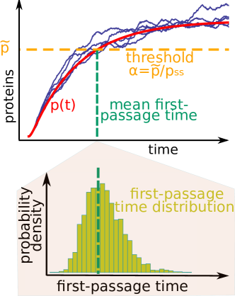
Figure 2: Definition of the threshold-crossing problem. When a gene is switched on at time $t=0$ the average protein level (red continuous line) approaches the steady state with the dynamics described by Eq. 2. Since gene expression is a stochastic process, individual trajectories fluctuate around the mean behavior, as illustrated by stochastic simulations (blue lines). The distribution of times of crossing a fixed protein level $\tilde{p}$ (orange horizontal dashed line) is the first-passage time distribution (histogram) representing the variabilty in reaching a certain level of expression. The average first-passage time can be directly deduced from the deterministic mean dynamics (green vertical dashed line).

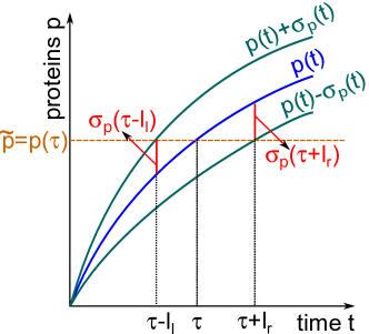
Figure 3: Scheme of the geometric relations at the basis of the analytical estimate of timing fluctuations. The average protein level $p(t)$ rises after induction at time $t=0$. The dynamics depends on the specific regulations acting on the gene. The time evolution of protein fluctuations is captured by the dynamics of the region at one standard deviation from the mean, defined by the curves $p(t)\pm\sigma_{p}(t)$. The time necessary to these curves to cross a fixed threshold $\tilde{p}$ gives an estimate of the variability in the FPT.

The threshold-crossing problem for gene expression is represented in Fig. 2. After induction, the level of gene expression rises with a specific dynamics $p(t)$ and approaches the steady-state $p_{ss}$ for long times. We want to evaluate the time necessary to reach a target level of expression $\tilde{p}$, and in particular its fluctuations. Mathematically, the problem of determining the time required for a stochastic process to reach a certain value falls into the category of first-passage time (FPT) problems Kampen2007 . Usually, FPT problems are difficult to treat analytically. Indeed, previous attempts of evaluating the FPT distribution in the context of gene expression were based on numerical approximations Shahrezaei2008 ; Murugan2011 , or on simplified processes, for example neglecting protein degradation Singh2014 . Here, we take a different approach. Our goal is to provide a rough but simple analytical estimate of the FPT noise that allows to identify and intuitively understand some of its general properties. To this aim, the geometrical arguments illustrated in Fig. 3 can be used. Fluctuations around the dynamics of the average protein level $p(t)$, which for constitutive expression is described by Eq. 2, are quantified by considering the region at a standard deviation distance from the mean behavior, defined by the two curves $p(t)\pm\sigma_{p}(t)$ shown in Fig. 3. A crossing threshold $\tilde{p}$ defines the dimensionless parameter $\alpha=\tilde{p}/p_{ss}$ and the corresponding mean FPT $\tau$. The two trajectories $p(t)\pm\sigma_{p}(t)$ cross the threshold $\tilde{p}$ at the time points $\tau-l_{l}$ and $\tau+l_{r}$ respectively. The time interval $[\tau-l_{l},\tau+l_{r}]$ can be considered as an estimate of the variability in the FPT. In particular, an approximation of the standard deviation of the FPT is given by the average value $\sigma_{t}(\tilde{p})\simeq\frac{l_{r}+l_{l}}{2}$, and this quantity can be calculated explicitily as a function of the known parameters of the process. Figure 3 shows that two geometric relations hold:

$$\sigma_{p}(\tau+l_{r})~{} = ~{}p(\tau+l_{r})-p(\tau)$$

$$\sigma_{p}(\tau-l_{l})~{} = ~{}p(\tau)-p(\tau-l_{l})\ .$$ (4)

These expressions can be Taylor expanded around the mean FPT $\tau$

$$\sigma_{p}(\tau)+\frac{d}{dt}\sigma_{p}(t)\Big{|}_{\tau}l_{r}+...~{} = ~{}\frac{dp(t)}{dt}\Big{|}_{\tau}l_{r}+...$$

$$\sigma_{p}(\tau)-\frac{d}{dt}\sigma_{p}(t)\Big{|}_{\tau}l_{l}+...~{} = ~{}\frac{dp(t)}{dt}\Big{|}_{\tau}l_{l}+...\ .$$ (5)

Considering the first-order expansion and generalizing to all possible threshold levels $p$ and their corresponding average FPT $t$, we obtain a general relation between the variability in the FPT $\sigma_{t}(p)$, the protein level variability at that time $\sigma_{p}(t)$, and the average dynamics $p(t)$:

$$\sigma_{t}(p)\simeq\frac{l_{r}+l_{l}}{2}\simeq\sigma_{p}(t)\frac{dp(t)}{dt}\Bigl{[}\left(\frac{dp(t)}{dt}\right)^{2}-\left(\frac{d\sigma_{p}(t)}{dt}\right)^{2}\Bigr{]}^{-1}$$ (6)

If the variability in the protein level is approximately constant in time, the above expression further simplifies to

$$\sigma_{t}(p)\simeq\left(\frac{dp(t)}{dt}\right)^{-1}\sigma_{p}(t)$$ (7)

an equation reminiscent of the classic “propagation of uncertainty” in statistics. Equations 6 and 7 can be easily reformulated in terms of the CV. In particular, the lowest order approximation of the CV of the FPT is

$$CV_{t}(p)\simeq\frac{p(t)}{t}\left(\frac{dp(t)}{dt}\right)^{-1}CV_{p}(t).$$ (8)

Note that $p(t)$ in this expression is the deterministic average dynamics of the process, and $t$ is the average time if takes for $p(t)$ to reach a generic fixed value $p$. This relation between noise in the protein level and noise in the timing of a threshold crossing is quite general (although approximate), since it does not require particular assumptions about the process in analysis. Clearly, the caveat is that the time dependence of noise in the protein level have to be known, which can be a severe limitation given that an exact analytical solution is only known for constitutive expression Shahrezaei2008 (Eq. 3), while it has to be evaluated through numerical simulations even for simple regulatory schemes.

Optimal out-of-equilibrium protein level for time measurements

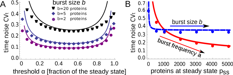
Figure 4: Minimum of noise in the first-passage time at intermediate protein levels. A) The coefficient of variation $CV_{t}$ of the FPT is reported as a function of the target expression level $\alpha$ (in units of the steady-state value). The analytical estimate in Eq. 8 (continuous lines) predicts with good precision the results of exact Gillespie simulations (symbols). Both curves show a minimum timing noise value for an intermediate level of expression, around $\alpha\simeq 0.55$. We verified that the presence of a minimum is robust with respect to the parameter values, as expected from Eq. 8. The plot considers different values of the burst size $b$, the key determinant of protein number fluctuations (Eq. 3), while keeping the steady state to a constant value ($ab=2000$ proteins). The mRNA halflife is 5 minutes and the protein halflife around 8 hours, roughly corresponding to dilution for bacteria in slow-growth conditions (see the Materials and Methods section for the biologically relevant range of the parameter values). B) Increasing the number of proteins produced (thus relaxing the constraint on the steady state value) lowers the noise in the timing fluctuations if expression is controlled at the transcriptional level, i.e., varying the burst frequency $a$. On the other hand, increasing the translation rate, and thus the burst size $b$, does not affect the timing noise. Lines represent the analytical predictions while dots are the results of Gillespie simulations.

This section addresses the role of the positioning of the threshold protein level in determining the FPT fluctuations. We consider the example of a transcription factor (TF) whose expression is turned on in response to an external stimulus. Typically, the dependence of the target expression on the TF concentration is sigmoidal Alon2007 ; Bintu2005a , triggering a response when the level of expression approximately matches the dissociation constant of the target. The dissociation constant is largely defined by the sequence specificity of the TF to the promoter Bintu2005 , and thus it is subject to evolutionary selection Ronen2002 ; Zaslaver2004 ; Yosef2011 . If noise in the timing is a variable with phenotypic relevance, the threshold level that triggers the target response may have been tuned so as to, for instance, minimise the noise in the FPT. Given a steady-state protein level $p_{ss}$ that the regulator dynamics will reach asymptotically, the system could select a threshold $\alpha$ with the smallest noise in the time “measured” by the target response. The question is how the FPT variability depends on the threshold level $\alpha$, and if an optimal strategy for controlling timing noise actually exists.

In the case of simple activation without further regulation (”constitutive”), the noise in the protein number is known analytically (Eq. 3), and thus Eq. 8 can be used as a first estimate of the FPT noise. In this approximation, the relative fluctuations in the crossing time are a function of the frequency $a$ and size $b$ of expression bursts, and of the threshold $\alpha$,

$$CV_{t}^{2}=\frac{\alpha}{a~{}b}\frac{1+b(2-\alpha)}{[(1-\alpha)log(1-\alpha)]^{2}}.$$ (9)

This approximate analytical expression shows a non-monotonous dependence on $\alpha$, and is in very good agreement with the results of exact stochastic simulations of the process (Fig. 4A). The noise in the FPT has a minimum at an intermediate level of protein expression, implying that the threshold position can actually be selected in order to minimise the noise in the “time measurement”. Intuitively, the presence of this minimum is the result of a trade-off between the noise at the protein level and the steepness of the increase in time of the average protein level, as described by Eq. 8. Both quantities are decreasing functions of the threshold position in the case $\eta\ll 1$. This can be easily observed by taking the time derivative of the average protein dynamics (Eq. 2) and by simply reformulating the protein noise in Eq 8 as

$$CV_{p}^{2}(\alpha)=\frac{1+b(2-\alpha)}{a~{}b~{}\alpha}.$$ (10)

For short times the protein noise is high, while for long times the noise propagation is particularly efficient. The optimal trade-off is in the intermediate region. The timing noise depends on the specifics of the gene in analysis, i.e., on the burst size $b$ and frequency $a$ (Eq. 9). However, the value of $\alpha$ at which this noise has a minimum shows no dependence on the transcription rate, thus on the burst frequency $a$ for a fixed protein lifetime, and a dependence on the burst size $b$ that is completely negligible in the regime $b\gg 1$, which is typically the case empirically as described in the Materials and Methods section. In fact, in this regime the minimum position takes a constant value, approximately halfway to the steady state:

$$\frac{dCV_{t}^{2}(\alpha)}{d\alpha}\Big{|}_{b\gg 1}=0\Rightarrow\alpha\simeq 0.55.$$ (11)

This value compares well to simulations (Figure 4A).

As expected, the protein noise level determines the absolute value of the timing fluctuations. In fact, if the same number of proteins is produced with burst sizes of different amplitudes both the noise at the protein level (Eq. 3) and the timing noise (Eq. 8 and Fig. 4A) increase.

Note that if the process is simply a birth-death Poisson process, which can be the relevant case if the regulator is a non-coding RNA, the FPT noise has analogously a minimum value, in this case at $\alpha=0.47$. This can be calculated by substituting the steady-state value $ab$ with the corresponding steady state $k/\gamma$ of the birth (rate $k$) and death (rate $\gamma$) process, and taking the limit $b\rightarrow 0$ in Eq. 9.

In the specific case of a burst size much larger than the threshold level (i.e., $b\gg\tilde{p}$), the problem of evaluating the FPT fluctuations greatly simplifies. In fact, in this specific case, the first transcription event nearly always leads to a burst of protein production that crosses the threshold. Therefore, the FPT distribution is well approximated by an exponential distribution with a single parameter $k_{m}$ (i.e., the transcription rate) as can be easily tested with stochastic simulations.

We considered so far stable proteins with a halflife longer than the cell cycle, which is typically the case in microorganisms Taniguchi2010 ; Shahrezaei2008 . However, few proteins, such as stress response regulators, are actively degraded by proteolyis Gottesman1996 , and protein halflife can be controlled in synthetic circuits Cameron2014 . For unstable proteins, the higher degradation rate $\gamma_{p}$ can be compensated by an increased transcription rate $k_{m}$ or translation rate $k_{p}$ in order to reach the same steady-state level of expression $ab$. In the first case, both the burst size $b=k_{p}/\gamma_{m}$ and frequency $a=k_{m}/\gamma_{p}$ remain constant, while in the second case the burst size increases to compensate the reduced frequency. Eqs. 9 shows that, for a fixed steady state $ab$, the minumum noise level (i.e., for $\alpha~{}\simeq 0.55$) does not change for unstable proteins transcribed more often, while timing become more noisy if the burst size is increased. The average FPT corresponding to the minimum noise level decreases as the protein becomes less stable since $t\simeq-log(1-\alpha)/\gamma_{p}$. Therefore, if a signal has to be transmitted reliably on very short time scales with respect to the cell cycle, a possible cellular strategy is boosting the protein degradation at the cost of making more transcripts to achieve a shorter average crossing time without an increase in its relative fluctuations.

On the other hand, given a fixed average value of the crossing time, one can ask whether the timing variability can be reduced by the cell by “paying the cost” of producing more proteins. Eq. 9 shows that increasing the transcription rate, and thus the burst frequency $a$, can indeed decrease the absolute value of fluctuations. On the other hand, the timing variability does not depend on the burst size for $b\gg 1$. Therefore, making more proteins in order to have a more precise crossing time is a possible strategy if the expression is increased at the transcriptional level, but does not work if the increase occurs at the translational level (Fig. 4B).

Role of autoregulation in controlling timimg fluctuations

This section addresses how the timing noise is affected by self-regulation of the gene. Gene autoregulation is widespread in both bacteria and eukaryotes and has relevant consequences on the gene expression dynamics and stochasticity CosentinoLagomarsino2007 ; Alon2007 . For example, negative transcriptional self-regulation speeds up the expression rise-time after induction Rosenfeld2002 and can reduce the cell-to-cell variability in the protein number at steady state Dublanche2006 , while positive autoregulation slows down the time of induction Maeda2006 , and increases stochastic fluctuations eventually leading to expression bimodality in a specific range of parameters Maeda2006 ; Becskei2001 .

Transcriptional regulation is described by multiplying the transcription rate of the target with a nonlinear function $F(p)$ of the level of expression of the regulator Alon2007 ; Bintu2005 . The empirical dependence is well captured by a Hill function Bintu2005a of the form:

$$F_{-}(p)~{} = ~{}\frac{1}{[1+(p/K)^{n}]}~{}~{}~{}\textrm{for negative autoregulation},$$

$$F_{+}(p)~{} = ~{}\frac{(p/K)^{n}}{[1+(p/K)^{n}]}~{}~{}~{}\textrm{for positive autoregulation}.$$ (12)

Here, the dissociation constant $K$ specifies the regulator level at which the production rate is half of its maximum value, while the Hill coefficient $n$ defines the degree of cooperativity of the regulator and thus the steepnes of the regulation curve.

To compare in a meaningful way different regulatory strategies, it is essential to precisely define the constraints and the criteria to put different circuits on equal footing Alon2007 ; Bosia2012 . For example, to show that negative transcriptional regulation speeds up the gene response to activation, its dynamics can be compared to the one of a constitutive gene with the same steady-state level of expression Alon2007 ; Rosenfeld2002 . We adopt the same approach, comparing different regulatory strategies while keeping fixed the final expression level. This can be achieved in practice by choosing the appropriate values of the regulation strengths (defined by the dissociation constants $K$ in Eqs. 12) and of the basal transcription rates $k_{m}$ for the three circuits. Given this constraint, the same average response time can be achieved by different types of autoregulation (positive or negative) or by a constitutive promoter by setting the crossing threshold at different positions. This is shown in Fig. 5A: the protein expression tends asymptotically to the same equilibrium level in the three circuits, and the same average FPT (vertical line) is measured by placing different thresholds ($\alpha_{0,+,-}$) because of the different dynamics of the average protein level $p(t)$ in the three circuits.

Figure 5B shows the ratio between the timing noise of the two self-regulations and the timing noise for constitutive expression. Depending on the average crossing time, different regulatory strategies have different noise properties. Around the time scale set by the protein halflife (cell-cycle time in bacteria) adding any type of autoregulation introduces larger timing fluctuations. On the other hand, if the crossing time is shorter than the cell cycle, smaller timing fluctuations can be achieved introducing negative self-regulation, while positive autoregulation reduces the timing noise for longer time scales. The scenario emerging from this result is that the type of regulation that can buffer timing fluctuations crucially depends on the time that the cell has to precisely “measure” with respect to the typical time scale of the process (protein halflife or cell-cycle time for stable proteins). The reduction or amplification of noise in the protein number at the steady state seems to be more directly associated to the sign of autoregulation, i.e., noise reduction for repression and noise amplification for activation Alon2007a . Instead, the noise properties of autoregulation are context dependent at the level of FPT fluctuations (Fig. 5B).

This effect can be understood qualitatively by looking at the dynamics of the protein level in Figure 5A, and considering Eq. 8 to connect noise at the protein level and timing noise. Now, the dynamics of $p(t)$ is strongly dependent on the type of regulation. The expression of a constitutive gene crosses an intermediate (with respect to the steady state) protein level at a time close to the protein halflife since $t\simeq-log(1-\alpha)/\gamma_{p}$, and this is the range where its timing noise is close to a minumum. On the other hand, for negative autoregulation this same timing corresponds to a protein level much closer to the steady-state value, where the derivative $dp(t)/dt$ is much smaller, and thus the fluctuations are strongly amplified at the timing level. The opposite is true for short times, where this derivative has a larger value if the gene is negatively autoregulated. Analogous observations hold for positive autoregulation. Clearly, at a quantitative level, the fact that autoregulation can significantly change the noise at the protein level plays an important role. However, the contribution from the deterministic dynamics seems dominant in most cases.

As previously discussed, positive self regulation can display bistability, and thus bimodality, in the protein level for specific parameter values Maeda2006 ; Becskei2001 . In this particular case, the protein expression level can converge to a stable no- or low-expression state or to a high-expression state depending on initial conditions. Assuming a threshold value between these two stable states and an initial condition of low expression, the timing of threshold crossing would be defined by the residence time in the low-expression state. Bistable circuits are typically found at the basis of cell-fate determination and phenotypic heterogeneity, for example in the context of bacterial persistence and competence Norman2015 , where noise-driven stochastic switches are relatively rare. Therefore, a bistable circuit seems a less well suited strategy to transmit signals within timescales comparable to the cell cycle and with a reliable timing, as in cell-cycle regulation or circadian clocks. As a consequence, we did not explore parameter regimes for which the positive feedback shows bistability. In this case, other mathematical tools can be used to estimate the fluctuations in the residence times Walczak2005 ; Assaf2011 .

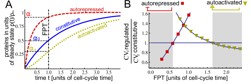
Figure 5: Timing noise can be reduced by different regulatory strategies in different time regimes. A) Setting of the comparison between regulatory strategies: we imposed the same steady state of expression for the three different circuits. A common average FPT (vertical line) is achieved by placing the target protein level $\alpha$ at a position that depends on the circuit type, corresponding to $\alpha_{0,+,-}$ in this example. Protein and mRNA lifetimes are defined as 5 min and 8 hours, while the steady-state number of proteins is $ab=2000$ as in Fig. 4. The average burst size has a value of $b=5$. The strengths of regulation are defined by the dissociation constants $K=1000$ and $K=90$ (proteins) for negative and positive autoregulation respectively. The Hill exponent $n=2$ was used for regulations. B) With the constraints shown in A, the timing noise for autorepression (squares) and autoactivation (triangles) are compared to the timing noise of a constitutive gene as a function of the average FPT value. Given the common final steady-state level of expression, each average FPT (x-axis) corresponds to a different threshold level for the three circuits (as illustrated in panel A) and to a different noise level. When the mean FPT is close to the protein halflife (or to the doubling time for stable proteins) both transcriptional autoregulations increase the timing noise (central region). The two shaded regions show the FPTs for which self-regulation works as a timing noise filter. In particular, autorepression reduces timing noise for time scales shorter than about 0.5 doubling times, while autoactivation is efficient in timing noise reduction on time scales longer than about 1.5 doubling times.

IV DISCUSSION

Our two most important results are the following. First, the fluctuations of the time necessary to reach a threshold expression level have a minimum value. This optimal threshold level of expression is approximately half the steady-state value. Thus, it does not naively coincide with a noise minimum in the protein number, which is instead monotonously decreasing while approaching the steady-state level. As a consequence, the level of noise in protein number does not directly translate into a level of timing fluctuations, since the out-of-equilibrium dynamics plays a non-negligible role. Therefore, the cellular strategies to control noise can be significantly different depending on what is exactly the biologically relevant variable, e.g., protein intracellular concentration or threshold-passing time.

Second, positive and negative transcriptional gene self-regulation can alter the level of timing fluctuations: the former reduces timing fluctuations at short times compared to one cell cycle (the system’s intrinsic time scale), while the latter reduces timing noise at large times. In other words, the role of autoregulation in controlling timing noise is context dependent. In the intermediate region (around one cell cycle), the absence of any regulation is the best strategy. Importantly, different regulatory strategies have been compared in a mathematically controlled way Alon2007 , thus measuring the timing variability given a fixed average crossing time and a fixed number of proteins produced. The cell can in principle further reduce the timing noise, as well as the noise at the protein level, by paying the cost of producing more proteins. However, we showed that also for timing noise this is effective only if the production is increased at the transcription level.

Giving up the ambition of a full analytical solution for the FPT problem, we provide a general approximate relation linking timing fluctuations and noise at the protein level that leads to a closed-form expression for the timing noise of constitutive expression. This expression was not employed in previous studies; we tested it with exact stochastic simulations, and appears to be useful in many regimes. Importantly, this simple estimate may be applicable to cellular first-passage time noise problems in more general contexts than the gene expression problem considered here, including protein modification, signal transduction, and titration, which has likely importance for cell-cycle progression Amodeo2016 ; Schmoller2015a The importance of this estimate is that it gives a clear intuition about general features of timing fluctuations. In particular, in our case we can capture and explain the fact that the timing noise shows a minimum value at a threshold expression level approximately half of the steady-state value. In the case of a transcription factor inducing a target gene, this translates into setting the value of the dissociation constant around half the steady-state level of the regulator. This general property can be used for the design of synthetic genetic circuits such as clocks and oscillators for which a precise timing is relevant Tigges2009 .

A recent interesting study also produced analytical estimates of the FPT fluctuations Singh2014 , but only in the specific case of gene expression in absence of protein degradation or dilution through growth. Although the results appear to be relevant for the case of lysis time variation in the bacteriophage lambda, they do not easily generalise to the classic scheme of gene expression in Fig. 1, which is more realistic for most genes. Indeed, as we showed, the intrinsic time scale defined by protein halflife plays an important role in shaping timing fluctuations.

Another study Shahrezaei2008 proposed an approach to estimate the FPT distribution based on numerical solutions of a renewal equation, but did not explored systematically the sources or controls of timing variability. A subsequent work Murugan2011 , focused on the role of the mRNA to protein lifetime (the parameter $\eta=\gamma_{p}/\gamma_{m}$) in shaping timing fluctuations for autoregulatory loops. Using a continuous approximation and numerical simulations, the authors showed that in these circuits timing fluctuations can be tuned by $\eta$. Here, we extend the list of the key variables determining timing fluctuations, and we show that different autoregulatory strategies can efficiently control timing noise at different time scales. Importantly, we also provide an analytical explanation of our results, based on a simple, although approximate, approach to evaluate timing fluctuations and intuitively understand some of its general properties.

While we only considered self-regulatory strategies, more complex genetic circuits can play an important role in shaping timing fluctuations. A recent theoretical analysis suggests for example that incoherent feedforward loops can be an efficient topology to dampen timing fluctuations Ghusinga2016 .

An important technical extension of the work presented here would be the inclusion of extrinsic fluctuations, i.e., fluctuations in the model parameters due to the variability of global factors affecting gene expression such as polymerases or ribosome concentrations Swain2002 . Extrinsic noise can be relevant especially for highly expressed genes Taniguchi2010 , and its effects on timing fluctuations is completely unknown. Unfortunately, the sources of extrinsic noise are still not fully understood, and analytical calculations easily become unfeasible in presence of parameter fluctuations. Therefore, this extension is out of the scope of the present work and will require an extensive exploration of the possible sources and functional forms of extrinsic noise and of its propagation at the timing level. Moreover, more complex models explicitly accounting for cell-cycle progression, DNA replication and cell division may be necessary to fully capture the details of expression timing fluctuations, especially if the time scales in analysis are short with respect to the cell cycle Bierbaum2015 ; Soltani2016 .

Importantly, fluctuations in the time necessary for a regulator to reach a threshold expression level may not be the only source of the overall timing noise. In fact, a regulator reaching a critical expression level also needs to be “sensed” by the downstream processes. For example, TFs have to find and bind target promoters in order to control their expression. This “reading process” takes some time and introduces additional timing variability. An order-of-magnitude estimate of reaction times points to the presence of a separation of time scales between the relatively slow change in a protein level due to transcription and translation and the faster kinetics of target search and binding/unbinding to promoters Alon2007 ; Swift2016 . More precisely, single-molecule experiments addressing the kinetics of TF search Li2009 , have shown that a single TF molecule can find its binding site in about 4 minutes Hammar2012 , and this search time is expected to reduce proportionally to the number of TFs Slutsky2004 . Hence, for TFs that are present in hundreds or thousands of copies, we expect these times to be negligible compared to changes in protein levels, which happen on a time scale of the order of the cell cycle. These observations support a prominent role of the regulator expression dynamics with respect to the reading process of its targets in establishing timing fluctuations, unless the TF copy number is very low and the threshold crossing time is relatively fast. This general consideration finds some experimental evidence in the context of yeast meiosis: the variability in the expression dynamics of a meiotic master TF was shown to be the dominant source of variability in the onset time of downstream targets (and thus on the resulting phenotipic variability) Nachman2007 . However, a generalization of our modelling framework to include downstream processes should be required in cases in which the out-of-equilibrium kinetics of TF binding plays a non negligible role in the observed expression dynamics Hammar2014 .

While the biologically relevant circuits are in general more complex than those considered here, we can speculate on the implications of our results in a wider context. It is interesting to notice that the promoter of the dnaA gene is repressed by its own protein DnaA, forming a negative self-loop Grant2011 . DnaA is responsible for the initiation of DNA replication in E. coli by promoting the unwinding of the double-strand DNA when its level reaches a certain threshold Skarstad2013 . The initiation timing have to be precisely regulated to couple cell growth and division with DNA replication Adiciptaningrum2015 , and this timing is clearly shorter than the cell-cycle time. Our analysis suggests that indeed negative self-regulation can help controlling the timing fluctuations on such a time scale.

Additionally, the importance of expression timing could be relevant for genes beyond cell-cycle and circadian clock regulators. In fact, several endogenous genes are expressed in a precise temporal order. This is the case for example for genes involved in flagellar biosynthesis Kalir2001 , or genes coding for enzymes in the aminoacid biosynthesis systems of E. coli Zaslaver2004 . This temporal order has been proposed as the result of an optimization process due to a trade-off between speed and cost of production Alon2007 ; Zaslaver2004 . Often the genetic network implementing this temporal order is composed by a single TF that triggers the response of a set of target genes at different threshold levels Alon2007 . If the delay between the expression of these genes has to be tightly tuned, timing fluctuations in reaching the different thresholds could be detrimental. Interestingly, many of these master TFs are autoregulated. For example the lrhA gene, a key regulator controlling the transcription of flagellar, motility and chemotaxis genes, shows positive autoregulation Lehnen2002 . On the other hand, some of the pathways in aminoacid synthesis are controlled by a single regulator with a negative self-loop Zaslaver2004 . It is tempting to speculate that this can be also due to regulation of timing noise and not only of its average value. In fact, the response of metabolic genes is known to be generally fast (order of minutes) Zaslaver2004 , while the complete formation of a functioning flagella is intuitively a more time consuming process. Ideally, experiments directly checking the timing variability for different values of the threshold, for example looking at the response in fluorescence of target promoters with different binding affinities, or measurements of the timing noise in presence or absence of autoregulation would be the perfect tests of our theoretical work.

V Funding

The work was partially supported by the Compagnia San Paolo grant GeneRNet.

VI ACKNOWLEDGEMENTS

We thank Matthew AA Grant for useful discussions.

VI.0.1 Conflict of interest statement.

None declared.

References

- (1) Pedraza, J. M. and Paulsson, J. (2007) Random timing in signaling cascades.. Mol Syst Biol, 3, 81.
- (2) Yurkovsky, E. and Nachman, I. (Mar, 2013) Event timing at the single-cell level.. Brief Funct Genomics, 12(2), 90–98.
- (3) Bean, J. M., Siggia, E. D., and Cross, F. R. (Jan, 2006) Coherence and timing of cell cycle start examined at single-cell resolution.. Mol Cell, 21(1), 3–14.
- (4) Eldar, A. and Elowitz, M. B. (Sep, 2010) Functional roles for noise in genetic circuits.. Nature, 467(7312), 167–173.
- (5) Yosef, N. and Regev, A. (Mar, 2011) Impulse control: temporal dynamics in gene transcription.. Cell, 144(6), 886–896.
- (6) Kuchina, A., Espinar, L., Çağatay, T., Balbin, A. O., Zhang, F., Alvarado, A., Garcia-Ojalvo, J., and Süel, G. M. (2011) Temporal competition between differentiation programs determines cell fate choice.. Mol Syst Biol, 7, 557.
- (7) Singh, A. and Dennehy, J. J. (Jun, 2014) Stochastic holin expression can account for lysis time variation in the bacteriophage .. J R Soc Interface, 11(95), 20140140.
- (8) Paulsson, J. (Jan, 2004) Summing up the noise in gene networks.. Nature, 427(6973), 415–418.
- (9) Raj, A. and van Oudenaarden, A. (Oct, 2008) Nature, nurture, or chance: stochastic gene expression and its consequences.. Cell, 135(2), 216–226.
- (10) Murugan, R. and Kreiman, G. (Sep, 2011) On the minimization of fluctuations in the response times of autoregulatory gene networks.. Biophys J, 101(6), 1297–1306.
- (11) Amir, A., Kobiler, O., Rokney, A., Oppenheim, A. B., and Stavans, J. (2007) Noise in timing and precision of gene activities in a genetic cascade.. Mol Syst Biol, 3, 71.
- (12) Nachman, I., Regev, A., and Ramanathan, S. (Nov, 2007) Dissecting timing variability in yeast meiosis.. Cell, 131(3), 544–556.
- (13) Young, J. W., Locke, J. C. W., Altinok, A., Rosenfeld, N., Bacarian, T., Swain, P. S., Mjolsness, E., and Elowitz, M. B. (Jan, 2012) Measuring single-cell gene expression dynamics in bacteria using fluorescence time-lapse microscopy.. Nat Protoc, 7(1), 80–88.
- (14) Bennett, M. R. and Hasty, J. (Sep, 2009) Microfluidic devices for measuring gene network dynamics in single cells.. Nat Rev Genet, 10(9), 628–638.
- (15) Long, Z., Olliver, A., Brambilla, E., Sclavi, B., Lagomarsino, M. C., and Dorfman, K. D. (Oct, 2014) Measuring bacterial adaptation dynamics at the single-cell level using a microfluidic chemostat and time-lapse fluorescence microscopy.. Analyst, 139(20), 5254–5262.
- (16) Paulsson, J. (2005) Model of stochastic gene expression. Phys. Life Rev, 2, 157–175.
- (17) Kaern, M., Elston, T. C., Blake, W. J., and Collins, J. J. (Jun, 2005) Stochasticity in gene expression: from theories to phenotypes.. Nat Rev Genet, 6(6), 451–464.
- (18) Bar-Even, A., Paulsson, J., Maheshri, N., Carmi, M., O’Shea, E., Pilpel, Y., and Barkai, N. (Jun, 2006) Noise in protein expression scales with natural protein abundance.. Nat Genet, 38(6), 636–643.
- (19) Shahrezaei, V. and Swain, P. S. (Nov, 2008) Analytical distributions for stochastic gene expression.. Proc Natl Acad Sci U S A, 105(45), 17256–17261.
- (20) Rosenfeld, N., Elowitz, M. B., and Alon, U. (Nov, 2002) Negative autoregulation speeds the response times of transcription networks.. J Mol Biol, 323(5), 785–793.
- (21) Taniguchi, Y., Choi, P. J., Li, G.-W., Chen, H., Babu, M., Hearn, J., Emili, A., and Xie, X. S. (Jul, 2010) Quantifying E. coli proteome and transcriptome with single-molecule sensitivity in single cells.. Science, 329(5991), 533–538.
- (22) Thattai, M. and van Oudenaarden, A. (Jul, 2001) Intrinsic noise in gene regulatory networks.. Proc Natl Acad Sci U S A, 98(15), 8614–8619.
- (23) Osella, M. and Lagomarsino, M. C. (Jan, 2013) Growth-rate-dependent dynamics of a bacterial genetic oscillator.. Phys Rev E Stat Nonlin Soft Matter Phys, 87(1), 012726.
- (24) Friedman, N., Cai, L., and Xie, X. S. (Oct, 2006) Linking stochastic dynamics to population distribution: an analytical framework of gene expression.. Phys Rev Lett, 97(16), 168302.
- (25) Schwanhausser, B., Busse, D., Li, N., Dittmar, G., Schuchhardt, J., Wolf, J., Chen, W., and Selbach, M. (May, 2011) Global quantification of mammalian gene expression control.. Nature, 473(7347), 337–342.
- (26) Shahrezaei, V., Ollivier, J. F., and Swain, P. S. (2008) Colored extrinsic fluctuations and stochastic gene expression.. Mol Syst Biol, 4, 196.
- (27) Klumpp, S., Zhang, Z., and Hwa, T. (Dec, 2009) Growth rate-dependent global effects on gene expression in bacteria.. Cell, 139(7), 1366–1375.
- (28) Gillespie, D. T. (December, 1976) A general method for numerically simulating the stochastic time evolution of coupled chemical reactions. Journal of Computational Physics, 22(4), 403–434.
- (29) van Kampen N.G. (2007) Stochastic Processes in Physics and Chemistry, Elsevier Science and Tecnology Books, .
- (30) Alon, U. (2007) An Introduction to System Biology, Chapman & Hall/CRC, Boca Raton FL, .
- (31) Bintu, L., Buchler, N. E., Garcia, H. G., Gerland, U., Hwa, T., Kondev, J., and Phillips, R. (Apr, 2005) Transcriptional regulation by the numbers: models.. Curr Opin Genet Dev, 15(2), 116–124.
- (32) Bintu, L., Buchler, N. E., Garcia, H. G., Gerland, U., Hwa, T., Kondev, J., Kuhlman, T., and Phillips, R. (Apr, 2005) Transcriptional regulation by the numbers: applications.. Curr Opin Genet Dev, 15(2), 125–135.
- (33) Ronen, M., Rosenberg, R., Shraiman, B. I., and Alon, U. (Aug, 2002) Assigning numbers to the arrows: parameterizing a gene regulation network by using accurate expression kinetics.. Proc Natl Acad Sci U S A, 99(16), 10555–10560.
- (34) Zaslaver, A., Mayo, A. E., Rosenberg, R., Bashkin, P., Sberro, H., Tsalyuk, M., Surette, M. G., and Alon, U. (May, 2004) Just-in-time transcription program in metabolic pathways.. Nat Genet, 36(5), 486–491.
- (35) Gottesman, S. (1996) Proteases and their targets in Escherichia coli.. Annu Rev Genet, 30, 465–506.
- (36) Cameron, D. E. and Collins, J. J. (Dec, 2014) Tunable protein degradation in bacteria.. Nat Biotechnol, 32(12), 1276–1281.
- (37) Cosentino Lagomarsino, M., Jona, P., Bassetti, B., and Isambert, H. (Mar, 2007) Hierarchy and feedback in the evolution of the Escherichia coli transcription network.. Proc Natl Acad Sci U S A, 104(13), 5516–5520.
- (38) Dublanche, Y., Michalodimitrakis, K., Kümmerer, N., Foglierini, M., and Serrano, L. (2006) Noise in transcription negative feedback loops: simulation and experimental analysis.. Mol Syst Biol, 2, 41.
- (39) Maeda, Y. T. and Sano, M. (Jun, 2006) Regulatory dynamics of synthetic gene networks with positive feedback.. J Mol Biol, 359(4), 1107–1124.
- (40) Becskei, A., Séraphin, B., and Serrano, L. (May, 2001) Positive feedback in eukaryotic gene networks: cell differentiation by graded to binary response conversion.. EMBO J, 20(10), 2528–2535.
- (41) Bosia, C., Osella, M., Baroudi, M. E., Corà, D., and Caselle, M. (2012) Gene autoregulation via intronic microRNAs and its functions.. BMC Syst Biol, 6, 131.
- (42) Alon, U. (Jun, 2007) Network motifs: theory and experimental approaches.. Nat Rev Genet, 8(6), 450–461.
- (43) Norman, T. M., Lord, N. D., Paulsson, J., and Losick, R. (2015) Stochastic Switching of Cell Fate in Microbes.. Annu Rev Microbiol, 69, 381–403.
- (44) Walczak, A. M., Onuchic, J. N., and Wolynes, P. G. (Dec, 2005) Absolute rate theories of epigenetic stability.. Proc Natl Acad Sci U S A, 102(52), 18926–18931.
- (45) Assaf, M., Roberts, E., and Luthey-Schulten, Z. (Jun, 2011) Determining the stability of genetic switches: explicitly accounting for mRNA noise.. Phys Rev Lett, 106(24), 248102.
- (46) Amodeo, A. A. and Skotheim, J. M. (2016) Cell-Size Control.. Cold Spring Harb Perspect Biol, 8(4).
- (47) Schmoller, K. M., Turner, J. J., Kõivomägi, M., and Skotheim, J. M. (Oct, 2015) Dilution of the cell cycle inhibitor Whi5 controls budding-yeast cell size.. Nature, 526(7572), 268–272.
- (48) Tigges, M., Marquez-Lago, T. T., Stelling, J., and Fussenegger, M. (Jan, 2009) A tunable synthetic mammalian oscillator.. Nature, 457(7227), 309–312.
- (49) Ghusinga, K. R., Dennehy, J. J., and Singh, A. (2016) Controlling noise in the timing of intracellular events: A first-passage time approach. bioRxiv,.
- (50) Swain, P. S., Elowitz, M. B., and Siggia, E. D. (Oct, 2002) Intrinsic and extrinsic contributions to stochasticity in gene expression.. Proc Natl Acad Sci U S A, 99(20), 12795–12800.
- (51) Bierbaum, V. and Klumpp, S. (Sep, 2015) Impact of the cell division cycle on gene circuits.. Phys Biol, 12(6), 066003.
- (52) Soltani, M., Vargas-Garcia, C. A., Antunes, D., and Singh, A. (Aug, 2016) Intercellular Variability in Protein Levels from Stochastic Expression and Noisy Cell Cycle Processes.. PLoS Comput Biol, 12(8), e1004972.
- (53) Swift, J. and Coruzzi, G. M. (Aug, 2016) A matter of time - How transient transcription factor interactions create dynamic gene regulatory networks.. Biochim Biophys Acta,.
- (54) Li, G.-W. and Elf, J. (Dec, 2009) Single molecule approaches to transcription factor kinetics in living cells.. FEBS Lett, 583(24), 3979–3983.
- (55) Hammar, P., Leroy, P., Mahmutovic, A., Marklund, E. G., Berg, O. G., and Elf, J. (Jun, 2012) The lac repressor displays facilitated diffusion in living cells.. Science, 336(6088), 1595–1598.
- (56) Slutsky, M. and Mirny, L. A. (Dec, 2004) Kinetics of protein-DNA interaction: facilitated target location in sequence-dependent potential.. Biophys J, 87(6), 4021–4035.
- (57) Hammar, P., Walldén, M., Fange, D., Persson, F., Baltekin, O., Ullman, G., Leroy, P., and Elf, J. (Apr, 2014) Direct measurement of transcription factor dissociation excludes a simple operator occupancy model for gene regulation.. Nat Genet, 46(4), 405–408.
- (58) Grant, M. A. A., Saggioro, C., Ferrari, U., Bassetti, B., Sclavi, B., and Cosentino Lagomarsino, M. (2011) DnaA and the timing of chromosome replication in Escherichia coli as a function of growth rate.. BMC Syst Biol, 5, 201.
- (59) Skarstad, K. and Katayama, T. (Apr, 2013) Regulating DNA replication in bacteria.. Cold Spring Harb Perspect Biol, 5(4), a012922.
- (60) Adiciptaningrum, A., Osella, M., Moolman, M. C., Cosentino Lagomarsino, M., and Tans, S. J. (2015) Stochasticity and homeostasis in the E. coli replication and division cycle.. Sci Rep, 5, 18261.
- (61) Kalir, S., McClure, J., Pabbaraju, K., Southward, C., Ronen, M., Leibler, S., Surette, M. G., and Alon, U. (Jun, 2001) Ordering genes in a flagella pathway by analysis of expression kinetics from living bacteria.. Science, 292(5524), 2080–2083.
- (62) Lehnen, D., Blumer, C., Polen, T., Wackwitz, B., Wendisch, V. F., and Unden, G. (Jul, 2002) LrhA as a new transcriptional key regulator of flagella, motility and chemotaxis genes in Escherichia coli.. Mol Microbiol, 45(2), 521–532.