Mirror winding number and helical edge modes in honeycomb lattice with hopping-energy texture

Abstract

We illustrate possible topological phases in honeycomb lattice with textures in electron hopping energy between nearest-neighboring sites and show that they are characterized by the mirror winding number intimately related to the chiral (or sublattice) symmetry. Analytic wave functions of zero-energy edge modes in ribbon geometry are provided, which are classified into even and odd sectors with respect to the mirror operation with the mirror plane perpendicular to the edge, and evolve into the topological helical edge states at finite momenta. Intriguingly our results demonstrate that in order to achieve the topological phase one can decorate the edge in a way adaptive to the bulk hopping texture. This paves a new way to tailoring graphene in the topological point of view.

Introduction— Currently topological states of matter are attracting much attention Hasan and Kane (2010); Qi and Zhang (2011). One aspect of the study is to elaborate classification of material phases using topological invariants. The other aspect is application oriented and topologically protected surface/edge modes are focused. While topology is a notion that is not limited by symmetry, symmetries enrich topological phase diagrams Kane and Mele (2005a, b); Kitaev (2009); Ryu et al. (2010); Fu (2011); Morimoto and Furusaki (2013); Shiozaki and Sato (2014). The quantum spin Hall effect in electron systems characteristic of time-reversal symmetry is the first example of topological state with $\mathbb{Z}_{2}$ topological index. However, if we attempt to design $\mathbb{Z}_{2}$ topological insulators in a system without spin, it is not straightforward to mimic a time-reversal operator squaring to $-1$, which plays a key role in the topological classification Ryu et al. (2010). A possible way to resolve this difficulty is to relax symmetry to an approximate one Wu and Hu (2015); Mousavi et al. (2015); Wu and Hu (2016), and it is found that sometimes a symmetry holding in a limited region in the Brillouin zone is sufficient to support desired topological phase.

Of various possibilities, modulating honeycomb lattice is expected to be fruitful, and pedagogical as well as learned from the lessons so far Haldane (1988); Kane and Mele (2005a, b); Guinea et al. (2010); Ezawa (2012); Liang et al. (2013). The idea was first demonstrated in a photonic crystal made of dielectric cylinders Wu and Hu (2015), which are aligned in a slightly distorted honeycomb structure, and then extended to electronic tight-binding (TB) model in honeycomb lattice with texture in hopping energy Wu and Hu (2016). When the hopping energy within hexagons is different from that between hexagons, one can think of molecular orbitals in the hexagonal artificial atoms, and meanwhile the K and K’ points are folded to the $\Gamma$ point in the first Brillouin zone. These molecular orbitals approximately play a role of spin, and an operator of pseudo time-reversal symmetry squaring to $-1$ is achieved. It was revealed that when the inter hexagon hopping energy is stronger than the intra one, a topological state mimicking the quantum spin Hall state with time-reversal symmetry can be achieved without resorting to the intrinsic spin degrees of freedom.

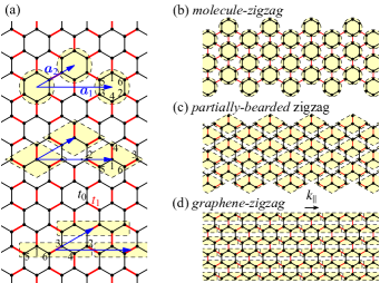
Figure 1: (Color online) (a) TB model in honeycomb lattice with texture in electron hopping energy between nearest-neighboring sites: $t_{0}$ (thin black bonds) and $t_{1}$ (thick red bonds) within and among hexagons encompassed by the dashed circles, and the two unit vectors $\bm{a}_{1}$ and $\bm{a}_{2}$. Small numbers in the unit cells represent the order for each site appearing in the basis set. (b,c,d) molecule-zigzag, partially-bearded and graphene-zigzag edge associated with the circular, rhombic and rectangular unit cell respectively denoted in (a) by dashed lines.

In this Letter, we elaborate the discussion on the electronic TB model on honeycomb lattice with texture in hopping energy between nearest-neighboring sites. We reveal that the topological state induced by the hopping texture can be characterized by the mirror winding number, a rigorous topological invariant intimately related to the chiral (or sublattice) symmetry. Analytic wave functions are provided for edge states at the $\Gamma$ point in ribbon geometry, which are classified into even and odd sectors with respect to the mirror operation with the mirror plane perpendicular to the edge, and evolve into the topological helical edge states at finite momenta, in agreement with the results of band calculations. Explicitly we find that when the intra-hexagon hopping energy is stronger (weaker) than the inter-hexagon one the so-called molecule-zigzag (partially-bearded) edge to honeycomb lattice yields gapless helical edge modes (see Fig. 1). Our discussions provide a new designing guideline for topological edge states, which paves a way to rich opportunities for applications.

Hamiltonian and chiral symmetry— We consider a TB Hamiltonian in honeycomb lattice

$$H=\sum_{\langle{ij}\rangle}t_{ij}c^{\dagger}_{i}c_{j}$$ (1)

where $c^{\dagger}_{i}$ ($c_{i}$) is the creation (annihilation) operator at site $i$, and $\langle{ij}\rangle$ denotes summation over the nearest-neighboring sites, with the hopping integral $t_{ij}$ modulated spatially (see Ref. Frank and Lieb, 2011 for a discussion on generic hopping textures). To be specific, we concentrate on the case that there are two hopping integrals $t_{0}$ and $t_{1}$, real and positive denoted by the thin black and thick red bonds in Fig. 1 respectively as in the previous work Wu and Hu (2016). Unit vectors associated with the hopping texture are given by $\bm{a}_{1}$ and $\bm{a}_{2}$. Because of the bipartite nature, the Hamiltonian can be rewritten into the form

$$H_{\bm{k}}=\begin{pmatrix}0&Q_{\bm{k}}\\ Q_{\bm{k}}^{\dagger}&0\end{pmatrix},$$ (2)

with a basis where the upper (lower) half is for A (B) sublattice and $Q_{\bm{k}}$ a 3$\times$3 matrix, irrespectively to the choice of unit cell [see Fig. 1(b,c,d)]. It is straightforward to confirm that the chiral operator $\gamma=\mathrm{diag}(1,-1)$ anticommutes with the Hamiltonian (2), manifesting the chiral symmetry (or sublattice symmetry) of the present system, which provides a powerful tool for one to tackle with the topological property.

Mirror winding number— Regarding the momentum $\bm{k}$ parallel to the unit vector $\bm{a}_{1}$ as a free parameter, the system can be viewed as an effective 1D model, to which one can assign the winding number Ryu et al. (2010). At the $\Gamma$ point $k_{\parallel}=0$, the Hamiltonian (2) can be reduced to the even and odd sectors by the mirror symmetry, with the mirror plane perpendicular to $\bm{a}_{1}$ [see Fig. 1(a)]. As far as the mirror plane is taken to be compatible with the hopping texture, the reduced Hamiltonian still has the chiral symmetry since the mirror operation commutes with $\gamma$, physically meaning that the mirror operation does not mix A and B sublattices. Then, it is possible to assign winding numbers for the even and odd sectors separately Morimoto and Furusaki (2013); Shiozaki and Sato (2014), which constitutes the mirror winding number $(n_{+},n_{-})$.

Table 1: Mirror winding number $(n_{+},n_{-})$ at $k_{\parallel}=0$. with $\delta\equiv t_{1}-t_{0}$ which are defined in Fig. 1(a).

$(n_{+},n_{-})$	$\delta>0$	$\delta<0$
molecule-zigzag	(1,$-1$)	(0,0)
partially-bearded	(0,0)	($-1$,1)
graphene-zigzag	(1,0)	(0,1)

In general, a winding number depends on how the unit cell is taken which determines the way momentum appearing in the Hamiltonian. Explicitly we consider three kinds of unit cell and the associated edges, noting that the edge should not destroy the unit cell for the purpose of discussion on edge states protected by the bulk topology Kariyado and Hatsugai (2013). The first unit cell is the circular one in Fig. 1(a), and the corresponding edge is given in Fig. 1(b) Klein and Bytautas (1999), which we call molecule-zigzag edge since a hexagonal cluster can be regarded as an artificial molecule Wu and Hu (2015, 2016). In this case one has

$$Q_{\bm{k}}=\begin{pmatrix}t_{1}X\bar{Y}^{2}&t_{0}&t_{0}\\ t_{0}&t_{1}\bar{X}Y&t_{0}\\ t_{0}&t_{0}&t_{1}Y\end{pmatrix}$$ (3)

where $X=e^{i\bm{k}\cdot\bm{a}_{1}}$ and $Y=e^{i\bm{k}\cdot\bm{a}_{2}}$. With the mirror symmetry at $k_{\parallel}=0$ , $Q_{\bm{k}}$ is decomposed into

$$Q^{+}_{k_{\perp}}=\begin{pmatrix}t_{1}\bar{Y}^{2}&\sqrt{2}t_{0}\\ \sqrt{2}t_{0}&t_{0}+t_{1}Y\end{pmatrix},\quad Q^{-}_{k_{\perp}}=t_{1}Y-t_{0},$$ (4)

with $+$ and $-$ for the even and odd sector respectively upon the mirror operation. One has nonzero winding numbers in both even and odd sectors $(n_{+},n_{-})=(1,-1)$ for $t_{1}>t_{0}$, and zero ones for $t_{1}<t_{0}$ (see appendix for details), which is consistent with the conclusion in the previous work Wu and Hu (2016).

The second unit cell is the rhombic one in Fig. 1(a), and the associated edge is given in Fig. 1(c) Klein and Bytautas (1999), which we called partially-bearded edge since the top edge is constructed by adding one extra lattice site every three sites at the zigzag edge known in the study of graphene. Note that with this unit cell the top and bottom edges of a ribbon system have different shapes. In this case, one has

$$Q_{\bm{k}}=\begin{pmatrix}t_{1}&t_{0}&t_{0}\\ t_{0}Y&t_{1}&t_{0}X\bar{Y}\\ t_{0}\bar{X}Y&t_{0}\bar{Y}&t_{1}\end{pmatrix},$$ (5)

which is decomposed into the even and odd sectors as

$$Q^{+}_{k_{\perp}}=\begin{pmatrix}t_{1}&\sqrt{2}t_{0}\\ \sqrt{2}t_{0}Y&t_{1}+t_{0}\bar{Y}\end{pmatrix},\quad Q^{-}_{k_{\perp}}=t_{1}-t_{0}\bar{Y}.$$ (6)

We have $(n_{+},n_{-})=(-1,1)$ for $t_{1}<t_{0}$ and zero winding number for $t_{1}>t_{0}$ (see appendix for details), in contrary to the first case.

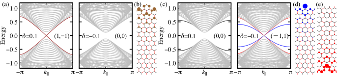
Figure 2: (a,c) Band structures of a ribbon system for molecule-zigzag edge and partially-bearded edge, with the mirror winding numbers $(n_{+},n_{-})$ indicated. In (a) the helical edge states are highlighted by the brown (dark) dispersions for $\delta=0.1$ with double degeneracy, whereas in (c) the blue (red) dispersions are for the helical edge states localized at the top (bottom) edge, with the corresponding real-space distribution of wave function $|\psi_{i}|^{2}$ displayed in (b,d,e). The gray lines in (a) and (c) are for bulk states. The black (dark) lines in (c) for $\delta=0.1$ represents edge states whose origin is not topology. The ribbon is infinitely long along $\bm{a}_{1}$ with periodic boundary condition and contains 40 unit cells along $\bm{a}_{2}$.

For the sake of comparison, a third unit cell is also considered as the rectangular one in Fig. 1(a), corresponding to the graphene-zigzag edge given in Fig. 1(d). It is easy to check that $(n_{+},n_{-})=(1,0)$ for $t_{1}>t_{0}$ and $(n_{+},n_{-})=(0,1)$ for $t_{1}<t_{0}$ (see appendix materials for details). Armchair edge is also well known in the study of graphene. It is easy to check that one cannot assign the mirror winding number for armchair edge, since the mirror operation mixes A and B sublattices, which corresponding the absence of gapless helical edge states.

Table 1 summarizes the mirror winding number $(n_{+},n_{-})$ for the three cases considered above. For molecule-zigzag and partially-bearded edges, the states for $\delta>0$ and $\delta<0$ with $\delta\equiv(t_{1}-t_{0})/t_{0}$ can be distinguished topologically in terms of the mirror winding number, but indistinguishable by the total winding number $n_{\rm tot}=n_{+}+n_{-}$; for graphene-zigzag edge, we have $n_{\text{tot}}=1$ irrespective of the sign of $\delta$. While the mirror winding number is only defined at $k_{\parallel}=0$, the total winding number $n_{\rm tot}$ is well-defined for any momentum, and is conserved as far as the bulk gap is not closed. Because a nonzero winding number specifies a zero-energy edge state, one can conclude that there is no zero-energy edge state for molecule-zigzag and partially-bearded edges at $k_{\parallel}\neq{0}$, whereas a zero-energy edge state for graphene-zigzag edge at any momentum, which is naturally connected to the discussion for graphene without hopping texture Ryu and Hatsugai (2002). To close this section, we notice that mirror winding numbers have been discussed recently for several other systems Zhang et al. (2013); Yang et al. (2014); Chiu and Schnyder (2015).

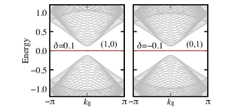
Figure 3: (Color online) Same as Fig. 2(a) except for that graphene-zigzag edge is adopted. The flat edge modes are highlighted by the brown color.

Band structure in ribbon geometry— Now let us evaluate the band structures of a ribbon system long and periodic in the direction parallel to $\bm{a}_{1}$ and of open boundaries in the perpendicular direction with the edge shapes illustrated in Fig. 1. As shown in Fig. 2, in the case of molecule-zigzag edge we find two doubly-degenerate dispersive modes associated with helical edge states localized at the top and bottom edges for $\delta>0$. The existence of two dispersive helical edge states at one edge with zero-energy gap at $k_{\parallel}=0$ are in accordance with $(n_{+},n_{-})=(1,-1)$ at $k_{\parallel}=0$ and $n_{\rm tot}=0$ for any momentum. For $\delta<0$ there is no edge mode as expected from the absence of mirror winding number in this case. For partially-bearded edge with $\delta<0$, we observe two dispersive modes associated with helical edge states at each of the two edges as shown in Fig. 2 in accordance with the mirror winding number (see Table I). In contrary to molecule-zigzag edge, in the case of partially-bearded edge the helical edge states at the top and bottom edges are not degenerate due to the absence of symmetry with respect to the middle line of ribbon. In contrast to the above results, for graphene-zigzag edge there is a dispersionless flat edge mode for both $\delta>0$ and $<0$ as shown in Fig. 3, known for long time in zigzag-edged graphene without hopping texture Fujita et al. (1996), which is in accordance with $n_{\rm tot}=1$ for any momentum $k_{\parallel}$ (see Table I).

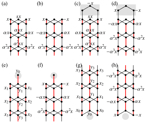
Figure 4: (Color online) Schematic pictures of the ansatz for the effective 1D model at $k_{\parallel}=0$: (a,b) for graphene-zigzag edge, (c,d) for molecule-zigzag edge, (e,f)/(g,h) for the top/bottom edge of partially-bearded edge. (a,c,e,g)/(b,d,f,h) are for the even/odd solutions with respect to mirror operation. The shaded regions for graphene-zigzag and partially-bearded edges can be regarded as decorations to graphene-zigzag edge.

Analytic wave functions of zero-energy edge modes— The effect of edge decoration becomes more obvious when we look into the detailed wave functions of zero-energy edge modes. Taking advantage of the chiral symmetry, the wave functions of zero-energy edge modes can be derived analytically based on the ansatz $\Psi_{A}=(\psi_{A},0)$ or $\Psi_{B}=(0,\psi_{B})$, which have finite weights only on either A or B sublattice. Since we focus on $k_{\parallel}=0$, the system is reduced to an effective 1D model as illustrated in Fig. 4. The key point is that, because of the mirror symmetry, the solutions can be classified by the parity with respect to the mirror operation, which puts constraints on and help us find the ansatz solutions (see Fig. 4).

Let us begin with the even-parity solution for graphene-zigzag edge as given in Fig. 4(a), which is symmetric with respect to the central column. Since the second site on the left (or right) column is connected to three sites, in order to have a nontrivial zero-energy mode with $x\neq 0$, one needs to require $(s+\alpha)t_{0}+t_{1}=0$ Nakada et al. (1996); Potasz et al. (2010). In the same way, from the fourth site on the central column, one has $2t_{0}+\alpha{s}t_{1}=0$. These two equations are satisfied by $\alpha=-\beta+\sqrt{\beta^{2}+1/\beta}$ and $s=-\beta-\sqrt{\beta^{2}+1/\beta}$ with $\beta\equiv(1+\delta)/2$. The solution is physically meaningful in the present case only when it decays from the edge into the bulk, namely $\alpha<1$, which is achieved by $\delta>0$. For the odd-parity solution given in Fig. 4(b), the ansatz gives a solution with $\alpha=1+\delta$ by inspection noting that the wave function is zero at the central column due to symmetry. A meaningful edge state therefore exists for $\delta<0$. These results are in accordance with the winding numbers summarized in Table I.

Next we check molecule-zigzag edge. As can be seen in Fig. 4(c), the even-parity solution in this case is essentially the same as that given in Fig. 4(a) for graphene-zigzag edge, for which one has a physical solution for $\delta>0$. On the other hand, for the odd-parity solution Fig. 4(d), the ansatz gives a solution with $\alpha=1/(1+\delta)$, which is physical for $\delta>0$. That is, the even- and odd-parity solutions are both physical when and only when $\delta>0$, matching the mirror winding number in Table I.

The partially-bearded edge is different from the above two cases in the sense the top and bottom edges in ribbon geometry is asymmetric with respect to the middle line of the ribbon [see Fig. 4(e) vs. (g) and (f) vs. (h)]. The odd-parity solutions in Figs. 4(f) and 4(h) are the same as the one for graphene-zigzag edge in Fig. 4(b), which are physical for $\delta<0$. For the even-parity solutions as given in Figs. 4(e) and (g), one expects that they are physical for $\delta<0$ judging from the mirror winding number in Table I, which can be proven with some algebra (see appendix).

One can derive molecule-zigzag edge by adding three sites as shown by the shade parts in Figs. 4(c) and (d) to graphene-zigzag edge, whereas partially-bearded edges are obtained by adding or deleting one site [see the shade parts in Figs. 4(e-h)]. It is then interesting to observe that the decoration of graphene-zigzag edge leading to molecule-zigzag (partially-bearded) edge only affects the odd-parity (even-parity) solution. For graphene-zigzag edge, one has one zero-energy mode for both $\delta>0$ and $\delta<0$. The decoration to graphene-zigzag edge then yields two zero-energy modes for $\delta>0$ ($\delta<0$) for molecule-zigzag (partially-bearded) edge, and suppresses the zero-energy mode for $\delta<0$ ($\delta>0$). The coexisting zero-energy even- and odd-parity solutions at $\Gamma$ point are mixed for $k_{\parallel}\neq 0$, where the mirror symmetry is no longer effective. Because of the parity difference, the coupling is linear in $k_{\parallel}$ and generates two linearly dispersive modes, which are nothing but the helical edge modes shown in Figs. 2.

Discussions — In the previous workWu and Hu (2016), the parameter regime $t_{1}<t_{0}$ was regarded as topologically trivial. However, as summarized in Table I this parameter regime supports a state characterized by nonzero mirror winding number. The difference comes from the different choices of unit cell: in the previous work the circular unit cell was taken, while the rhombic one is revealed to be appropriate (see Fig. 1). The way of taking unit cell is more than a convention in the present approach for realizing topological states based on hopping texture, since the existence of topological edge modes, and thus whether the system is topological or trivial, crucially relies on the shape of edge which is uniquely related to the unit cell. In this sense, the present work illuminates a way to realize topological states by edge decoration, which is expected very useful for tailoring graphene.

To summarize, topological phases in honeycomb lattice induced by texture in hopping energy between nearest-neighboring sites are characterized in terms of the mirror winding number, a rigorous topological invariant intimately related to the chiral (or sublattice) symmetry. Analytic wave functions are provided for zero-energy edge modes at the $\Gamma$ point, which evolve into the dispersive helical edge states at finite momenta. Explicitly, when the intra-hexagon hopping energy is stronger (weaker) than the inter-hexagon one, the molecule-zigzag (partially-bearded) edge to honeycomb lattice yields gapless helical edge modes. The present work provides a new designing guideline for topological edge states adaptive to the bulk hopping texture, which may pave a way to tailoring graphene in the topological point of view.

Appendix A Appendix

A.1 Armchair Edge

Mirror symmetry also exists for the armchair edge, a case well studied for graphene. However, considering the way to take unit cell compatible with armchair edge as displayed in Fig. 5, one finds that the mirror operation perpendicular to armchair edge does not commute with the chiral operator $\gamma$ defined in the main text, since the mirror operation in this case mixes A and B sublattices. Therefore, no mirror winding number can be assigned in this case, and as the result, no zero-energy edge modes exist for a ribbon with armchair edge, which agrees with the band calculation as shown in Fig. 5.

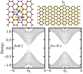
Figure 5: Same as Fig. 2 in the main text except for that armchair edge is adopted, and that the width is 20 unit cells along $\bm{a}^{\prime}_{2}$.

A.2 Evaluation of the Winding Number

Here we provide some details for the evaluation of winding numbers. Let us consider an effective 1D model constructed from a 2D model such as that given in the main text [see Eq. (2) in main text]

$$H_{k_{\parallel},k_{\perp}}=\begin{pmatrix}0&Q_{k_{\parallel},k_{\perp}}\\ Q^{\dagger}_{k_{\parallel},k_{\perp}}&0\end{pmatrix}$$ (7)

by regarding $k_{\parallel}$ as a free parameter. Then, the winding number $w$ is evaluated as Mizushima et al. (2016)

$$w =\frac{1}{4\pi{i}}\int_{0}^{2\pi}\mathrm{tr}\Bigl{[}\gamma{H}_{k}^{-1}\frac{dH_{k}}{dk}\Bigr{]}dk$$

$$=-\frac{1}{2\pi}\int_{0}^{2\pi}\frac{d}{dk}\arg(\det{Q}_{k})dk$$ (8)

with $k_{\perp}$ denoted by $k$ and $k_{\parallel}$ suppressed for clarity, where the second line follows from the relations

$$H_{k}^{-1}=\begin{pmatrix}0&(Q^{\dagger}_{k})^{-1}\\ Q_{k}^{-1}&0\end{pmatrix},$$ (9)

and $\mathrm{tr}Q^{-1}_{k}dQ_{k}=d\log\det{Q}_{k}$. Physically, Eq. (8) detects how $\det{Q}_{k}$ winds about the origin of the complex plane while $k$ evolves from $0$ to $2\pi$.

A.2.1 Mirror winding number for molecule-zigzag edge

The winding number for molecule-zigzag edge in the odd sector $n_{-}=-1$ for $t_{1}>t_{0}$, whereas $n_{-}=0$ for $t_{1}<t_{0}$ can be obtained straightforwardly from the second equality in Eq. (4) in the main text Rice and Mele (1982). For the even sector, one can see that, for $t_{1}=0$, $n_{+}=0$ since there is no momentum dependence in $Q^{+}_{k_{\perp}}$ in the first equality of Eq. (4) in the main text. This topological property remains unchanged in the whole regime $t_{1}<t_{0}$ where the gap always keeps open. On the other hand, for $t_{0}=0$, one has $n_{+}=1$ since one component of $Q^{+}_{k_{\perp}}$ winds twice about the origin of the complex plane as $k_{\perp}$ evolves from 0 to $2\pi$, while the other component winds once in the opposite direction. This winding number also remains the same for the whole regime $t_{1}>t_{0}$. One can confirm this intuitive discussion by plugging

$$\det{Q^{+}_{k_{\perp}}}=t_{1}\bar{Y}^{2}(t_{0}+t_{1}Y)-2t_{0}^{2}$$ (10)

into Eq. (8) and performing integration. The resultant winding numbers are summarized in Table I in the main text.

A.2.2 Mirror winding number for partially-bearded edge

Next we consider partially-bearded edge. For the odd sector the analysis is again obvious, noticing that in the second equality of Eq. (6) in the main text, $t_{0}$ and $t_{1}$ switch their positions from those in Eq. (4), which yields $n_{-}=1$ for $t_{1}<t_{0}$, whereas $n_{-}=0$ for $t_{1}>t_{0}$. For the even sector, we have

$$\det{Q}_{k_{\perp}}^{+}=t_{1}(t_{1}+t_{0}\bar{Y})-2t_{0}^{2}Y.$$ (11)

Then, it is clear that one has $n_{+}=0$ for $t_{1}>t_{0}$ as can be seen from the limit $t_{0}=0$, while $n_{+}=-1$ seen from the limit $t_{1}=0$. This of course can be confirmed by directly performing integration in Eq. (8).

A.2.3 Mirror winding number for graphene-zigzag edge

It is straightforward to see that for graphene-zigzag edge, one has

$$Q_{\bm{k}}=\begin{pmatrix}t_{1}X\bar{Y}&t_{0}&t_{0}\\ t_{0}&t_{1}\bar{X}&t_{0}\bar{Y}\\ t_{0}&t_{0}\bar{Y}&t_{1}\end{pmatrix},$$ (12)

which yields

$$Q^{+}_{k_{\perp}}=\begin{pmatrix}t_{1}\bar{Y}&\sqrt{2}t_{0}\\ \sqrt{2}t_{0}&t_{1}+t_{0}\bar{Y}\end{pmatrix},\quad Q^{-}_{k_{\perp}}=t_{1}-t_{0}\bar{Y}.$$ (13)

Again, the winding number in the odd sector is obvious. For the even sector, using

$$\det{Q}^{+}_{k_{\perp}}=t_{1}\bar{Y}(t_{1}+t_{0}\bar{Y})-2t_{0},$$ (14)

one can obtain $n_{+}=1$ for $t_{1}>t_{0}$ by considering the limit case $t_{0}=0$, and $n_{+}=0$ for $t_{1}<t_{0}$ by taking the limit $t_{1}=0$.

A.3 Analytic Solution for Partially-Bearded Edge

Here we discuss the wave functions of the even-parity zero-energy modes for partially-bearded edge. For the top edge as shown in Fig. 4(e) in the main text, in order to have a nontrivial solution one has to require $2t_{0}x_{j+1}+t_{1}y_{j}=0$ (see the central column) and $t_{1}x_{j+1}+t_{0}y_{j+1}+t_{0}x_{j}=0$ (see the left or right column) for $j>0$. They can be summarized into a matrix form

$$\begin{pmatrix}x_{j+1}\\ y_{j+1}\end{pmatrix}=A\begin{pmatrix}x_{j}\\ y_{j}\end{pmatrix},\quad A=\begin{pmatrix}0&-\beta\\ -1&2\beta^{2}\end{pmatrix},$$ (15)

with $\beta=(1+\delta)/2$ as defined in the main text, which gives

$$\begin{pmatrix}x_{n}\\ y_{n}\end{pmatrix}=A^{n-1}\begin{pmatrix}x_{1}\\ y_{1}\end{pmatrix}.$$ (16)

The two eigenvalues of the matrix $A$ are given by $\epsilon_{\pm}=\beta^{2}\pm\sqrt{\beta^{4}+\beta}$, which should satisfy $|\epsilon_{\pm}|<1$ in order to make the solution decaying into the bulk. This is guaranteed by $\delta<0$. The same discussions apply for the bottom edge shown in Fig. 4(g) in the main text.

References

- Hasan and Kane (2010) M. Z. Hasan and C. L. Kane, Rev. Mod. Phys. 82, 3045 (2010).
- Qi and Zhang (2011) X.-L. Qi and S.-C. Zhang, Rev. Mod. Phys. 83, 1057 (2011).
- Kane and Mele (2005a) C. L. Kane and E. J. Mele, Phys. Rev. Lett. 95, 146802 (2005a).
- Kane and Mele (2005b) C. L. Kane and E. J. Mele, Phys. Rev. Lett. 95, 226801 (2005b).
- Kitaev (2009) A. Kitaev, AIP Conf. Proc. 1134, 22 (2009).
- Ryu et al. (2010) S. Ryu, A. P. Schnyder, A. Furusaki, and A. W. W. Ludwig, New J. Phys. 12, 065010 (2010).
- Fu (2011) L. Fu, Phys. Rev. Lett. 106, 106802 (2011).
- Morimoto and Furusaki (2013) T. Morimoto and A. Furusaki, Phys. Rev. B 88, 125129 (2013).
- Shiozaki and Sato (2014) K. Shiozaki and M. Sato, Phys. Rev. B 90, 165114 (2014).
- Wu and Hu (2015) L.-H. Wu and X. Hu, Phys. Rev. Lett. 114, 223901 (2015).
- Mousavi et al. (2015) S. H. Mousavi, A. B. Khanikaev, and Z. Wang, Nature Commun. 6 (2015).
- Wu and Hu (2016) L.-H. Wu and X. Hu, Sci. Rep. 6, 24347 (2016).
- Haldane (1988) F. D. M. Haldane, Phys. Rev. Lett. 61, 2015 (1988).
- Guinea et al. (2010) F. Guinea, M. I. Katsnelson, and A. K. Geim, Nat. Phys. 6, 30 (2010).
- Ezawa (2012) M. Ezawa, Phys. Rev. Lett. 109, 055502 (2012).
- Liang et al. (2013) Q.-F. Liang, L.-H. Wu, and X. Hu, New J. Phys. 15, 063031 (2013).
- Frank and Lieb (2011) R. L. Frank and E. H. Lieb, Phys. Rev. Lett. 107, 066801 (2011).
- Kariyado and Hatsugai (2013) T. Kariyado and Y. Hatsugai, Phys. Rev. B 88, 245126 (2013).
- Klein and Bytautas (1999) D. J. Klein and L. Bytautas, J. Phys. Chem. A 103, 5196 (1999).
- Ryu and Hatsugai (2002) S. Ryu and Y. Hatsugai, Phys. Rev. Lett. 89, 077002 (2002).
- Zhang et al. (2013) F. Zhang, C. L. Kane, and E. J. Mele, Phys. Rev. Lett. 111, 056403 (2013).
- Yang et al. (2014) S. A. Yang, H. Pan, and F. Zhang, Phys. Rev. Lett. 113, 046401 (2014).
- Chiu and Schnyder (2015) C.-K. Chiu and A. P. Schnyder, J. Phys: Conf. Ser. 603, 012002 (2015).
- Fujita et al. (1996) M. Fujita, K. Wakabayashi, K. Nakada, and K. Kusakabe, J. Phys. Soc. Jpn. 65, 1920 (1996).
- Nakada et al. (1996) K. Nakada, M. Fujita, G. Dresselhaus, and M. S. Dresselhaus, Phys. Rev. B 54, 17954 (1996).
- Potasz et al. (2010) P. Potasz, A. D. Güçlü, and P. Hawrylak, Phys. Rev. B 81, 033403 (2010).
- Mizushima et al. (2016) T. Mizushima, Y. Tsutsumi, T. Kawakami, M. Sato, M. Ichioka, and K. Machida, J. Phys. Soc. Jpn. 85, 022001 (2016).
- Rice and Mele (1982) M. J. Rice and E. J. Mele, Phys. Rev. Lett. 49, 1455 (1982).