OU-HET 903

Entanglement entropy for free scalar fields in AdS

Sotaro Sugishita

Department of Physics, Osaka University, Toyonaka, Osaka, 560-0043, Japan

Abstract

We compute entanglement entropy for free massive scalar fields in anti-de Sitter (AdS) space. The entangling surface is a minimal surface whose boundary is a sphere at the boundary of AdS. The entropy can be evaluated from the thermal free energy of the fields on a topological black hole by using the replica method. In odd-dimensional AdS, exact expressions of the Rényi entropy $S_{n}$ are obtained for arbitrary $n$. We also evaluate 1-loop corrections coming from the scalar fields to holographic entanglement entropy. Applying the results, we compute the leading difference of entanglement entropy between two holographic CFTs related by a renormalization group flow triggered by a double trace deformation. The difference is proportional to the shift of a central charge under the flow.

1 Introduction

The study of entanglement entropy in quantum field theories began to give a microscopic explanation of the black hole entropy [1, 2, 3, 4, 5]. The area-law of the entanglement entropy of a region and its complement, which is also called geometric entropy, actually resembles the Bekenstein-Hawking entropy [6, 7, 8, 9]. Entanglement entropy is expected to be related to degrees of freedom in the system. For example, we can analytically calculate entanglement entropy for a single interval in (1+1)-dimensional conformal field theory [10, 11, 12], and it is proportional to the central charge of the CFT. However, it is generally difficult to directly compute entanglement entropy in higher dimensional CFTs and non-conformal field theories ( see, e.g., [13, 14, 15, 16] where entanglement entropy in free theories is evaluated). In order to know general properties of entanglement entropy, we should investigate examples where entanglement entropy is computed analytically. A natural extension is to consider QFTs in curved backgrounds such as black hole backgrounds [17], de Sitter space [18] and anti-de Sitter space (AdS) [19].

In this paper, we compute entanglement entropy for free massive scalar fields in AdS. Applying the result, we can evaluate quantum corrections of holographic entanglement entropy [20] as in [19]. The holographic entanglement entropy formula is proposed, in the context of the AdS/CFT correspondence [21], as a simple formula to compute entanglement entropy of a CFT with a gravity dual (see also [22, 23]). The formula states that the entanglement entropy of region $B$ in a CFT is, like the Bekenstein-Hawking entropy formula, proportional to the minimal area of a bulk surface $\Sigma$ that ends on the boundary of $B$ (see Fig 1),

$$S_{cl}(B)=\frac{\text{area}(\Sigma)}{4G_{N}},$$ (1.1)

where $G_{N}$ is bulk Newton’s constant. This formula is valid at the classical level (in the bulk). If the dual CFT is a large $N$ theory, the contribution of (1.1) corresponds to order $N^{2}$. In order to include the $1/N$ corrections in the CFT side, we need to consider quantum corrections to eq. (1.1). In other words, the formula (1.1) is the leading term in the $G_{N}$ expansion, which is order $G_{N}^{-1}$.

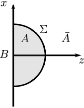
Figure 1: Minimal surface $\Sigma$ corresponding to the region $B$ in the boundary. The $z$-direction denotes the bulk direction, and $x$ are the spatial coordinates of the boundary. The region surrounded by $B$ and $\Sigma$ is denoted by $A$.

Faulkner, Lewkowycz and Maldacena (FLM) [27] propose that the $\mathcal{O}(G_{N}^{0})$ correction to the holographic entanglement entropy consists as follows

$$S_{q}(B)=S^{\text{bulk}}(A)+\delta\frac{\text{area}(\Sigma)}{4G_{N}}+\delta S_{\text{Wald}}+S_{c.t.}\,.$$ (1.2)

The first term $S^{\text{bulk}}(A)$ represents the entanglement entropy of quantum fields between a region $A$ and its complement $\bar{A}$ in the bulk. Here, $A$ is the region surrounded by $B$ and $\Sigma$ as in Fig. 1. The second term is the shift of the minimal area due to the change of the background because of quantum expectation values of matter fields. The term $\delta S_{\text{Wald}}$ denotes Wald-like entropy contributions arising from the expectation values of quantum fields. The last term $S_{c.t.}$ is introduced as the counter terms to cancel the bulk UV divergences.

In [19], Miyagawa, Shiba and Takayanagi investigate an example where the quantum corrections (1.2) give the leading contributions. They consider a gravity dual of a CFT perturbed by a relevant double trace deformation [29, 30, 31] and study the change of holographic entanglement entropy under a flow produced by the double trace deformation. In the gravity side, there is a massive scalar field dual to a single trace operator $\mathcal{O}$. The dimension of operator $\mathcal{O}$ is related to the mass $m$ of the scalar field [32, 33] as

$$\Delta_{\pm}=\frac{d-1}{2}\pm\nu,\quad\quad\nu=\sqrt{m^{2}\,\ell_{\text{AdS}}^{2}+\biggl{(}\frac{d-1}{2}\biggr{)}^{2}}\,,$$ (1.3)

where $d$ denotes the dimensions of AdS space and $\ell_{\text{AdS}}$ is the radius of AdS. When the mass of scalar field is in a certain range

$$-\biggl{(}\frac{d-1}{2}\biggr{)}^{2}<m^{2}\ell_{\text{AdS}}^{2}<-\biggl{(}\frac{d-1}{2}\biggr{)}^{2}+1\,,$$ (1.4)

that is, $0<\nu<1$, both dimensions $\Delta_{\pm}$ satisfy the unitarity bound $\Delta_{\pm}>(d-3)/2$ of $(d-1)$-dimensional CFT, and two corresponding boundary conditions of the scalar field in AdS are allowed [34]. One is the Dirichlet boundary condition corresponding to $\Delta_{+}$, and the other is the Neumann boundary condition corresponding to $\Delta_{-}$. If we start from a CFT, (we call CFT^(N)), where $\mathcal{O}$ has the dimension $\Delta_{-}$ and add a double trace deformation $\mathcal{O}^{2}$, which is relevant, the theory flows to another CFT (we call CFT^(D)) where the dimension of $\mathcal{O}$ is $\Delta_{+}$. In the dual gravity side, the difference of two theories is the boundary conditions of the scalar field. Thus, the leading contributions of holographic entanglement entropy (1.1) are the same for both theories. In addition, contributions from other fields in the bulk are not affected by the difference of the scalar boundary conditions at the 1-loop level. Therefore, if we consider the difference of entanglement entropy between CFT^(N) and CFT^(D), the leading difference comes from 1-loop contributions (1.2) of the scalar field.

The subregion $B$ in CFT is taken to be a half space in [19]. In the present paper, we take the subregion $B$ as a ball with radius $r_{0}$. In fact, if the subregion is a ball, the universal part of entanglement entropy is given by [35]

$$S^{univ}(B)=\left\{\begin{array}[]{ll}(-1)^{\frac{d-3}{2}}\,4\,a_{d-1}^{\ast}\log\frac{r_{0}}{\epsilon}&(d-1:\text{even})\\ (-1)^{\frac{d-2}{2}}\,2\pi\,a_{d-1}^{\ast}&(d-1:\text{odd})\\ \end{array}\right.\,,$$ (1.7)

where $\epsilon$ is a boundary UV cutoff, and $a_{d-1}^{\ast}$ agrees with the A-type trace anomaly $a$ in the case where $d-1$ is even (see also [36]). Since the shift of the central charge $a$ under the double trace deformation is computed at the leading order without AdS/CFT in [31], we can test the FLM proposal (1.2) by comparing the change of entanglement entropy with the result in [31]. We will evaluate, in odd-dimensional AdS_d $(3\leq d\leq 11)$, all terms in (1.2) except for $S_{c.t.}$, where we assume that $S_{c.t.}$ just cancels the bulk UV divergences of the other terms. The result is consistent with that expected from (1.7).

We also give explicit expressions of the Rényi entanglement entropy for free massive scalar fields in odd-dimensional AdS_d, by a purely field theoretic computation. We hope that our results serve as an example of the Rényi entropy for non-conformal theories.

This paper is organized as follows: In section 2 we summarize a method for computing entanglement entropy in AdS. In section 3, we compute entanglement entropy (and the Rényi entropy) for free massive scalar fields in odd-dimensional AdS using the heat kernels. In section 4, we evaluate 1-loop corrections of holographic entanglement entropy and find that the change of entanglement entropy under an RG flow by a double trace deformation is proportional to the shift of the A-type central charge. In section 5, we summarize our results and give some discussion.

2 Method for computing entanglement entropy in AdS

In this paper, we use the replica method to compute entanglement entropy in AdS, which is reviewed in subsection 2.1. Using the replica method, the Rényi entropy can be computed from a free energy on a replicated space. We will see that the free energy is given by a thermal free energy on the topological black hole in subsection 2.2. The fact also enables us to compute the modular Hamiltonian of the bulk fields. In subsection 2.4, we will confirm that the leading divergence of Rényi entropy satisfies the area-law for general dimensions and general mass.

2.1 Replica method

In this subsection, we review the replica method (see, e.g., [3, 11, 12]).

We consider a theory on $d$-dimensional AdS space, and compute entanglement entropy of a region $A$ for the ground state. The total density matrix of the ground state $\rho_{\text{tot}}$ can be represented as a path integral

$$\Bra{\phi_{1}(\vec{x})}\rho_{\text{tot}}\Ket{\phi_{2}(\vec{x})}=\frac{1}{Z_{1}}\int^{t_{E}=\infty}_{t_{E}=-\infty}\!\!\!\!\mathcal{D}\phi(t_{E},\vec{x})\,\delta(\phi(0_{-},\vec{x})-\phi_{1}(\vec{x}))\,\delta(\phi(0_{+},\vec{x})-\phi_{2}(\vec{x}))\,e^{-S_{E}}\,,$$ (2.1)

where $S_{E}$ is the Euclidean action and $Z_{1}$ is the partition function:

$$Z_{1}=\int^{t_{E}=\infty}_{t_{E}=-\infty}\!\!\!\!\mathcal{D}\phi(t_{E},\vec{x})\,e^{-S_{E}}\,.$$ (2.2)

Using the path integral representation, the reduced density matrix on the region $A$ is given by

$$\Bra{\phi_{1}^{A}(\vec{x})}\rho_{A}\Ket{\phi_{2}^{A}(\vec{x})}$$

$$=\frac{1}{Z_{1}}\int^{t_{E}=\infty}_{t_{E}=-\infty}\!\!\!\!\mathcal{D}\phi(t_{E},\vec{x})\,\prod_{\vec{x}\in A}\delta(\phi(0_{-},\vec{x})-\phi_{1}^{A}(\vec{x}))\,\delta(\phi(0_{+},\vec{x})-\phi_{2}^{A}(\vec{x}))\,e^{-S_{E}}\,.$$ (2.3)

Thus, we have

$$\operatorname{tr}_{A}\rho_{A}^{n}=\frac{Z_{n}}{Z_{1}^{n}}\,,$$ (2.4)

where $Z_{n}$ represents a path integral on $n$-sheeted covering space $\mathcal{M}_{n}$ which is obtained by sewing cyclically $n$ copies of the original Euclidean AdS space (EAdS) together along $A$. The Rényi entanglement entropy $S_{n}$ is then represented as

$$S_{n}\equiv\frac{\log\operatorname{tr}_{A}\rho_{A}^{n}}{1-n}=\frac{1}{1-n}(\log Z_{n}-n\log Z_{1})\,.$$ (2.5)

If we obtain the analytic continuation of $S_{n}$ to $\mathrm{Re}\,n>1$, the (von Neumann) entanglement entropy $S_{1}$ is computed as

$$S_{1}\equiv-\operatorname{tr}_{A}\rho_{A}\log\rho_{A}=\lim_{n\to 1}S_{n}\,.$$ (2.6)

2.2 Coordinate transformations and topological black hole

In the Poincaré coordinates, the metric of AdS space is given by

$${\mathrm{d}}s^{2}=\ell_{\text{AdS}}^{2}\frac{{\mathrm{d}}z^{2}-{\mathrm{d}}t^{2}+\sum_{i=1}^{d-2}{\mathrm{d}}x_{i}^{2}}{z^{2}}\,,$$ (2.7)

where $\ell_{\text{AdS}}$ is the radius of AdS_d. We also write the coordinates as

$$z=r\sin\theta,\,x_{i}=r\cos\theta\,\Omega_{i}$$ (2.8)

with

$$r>0,\,\quad\left\{\begin{array}[]{ll}0<\theta<\pi&(d=3)\\ 0<\theta<\pi/2&(d\geq 4)\\ \end{array}\right.\,,$$ (2.11)

where $\Omega_{i}$ denote coordinates of $(d-3)$-dimensional sphere. We consider the minimal surface $\Sigma$ corresponding to a ball region $B$ with radius $r_{0}$. One can find that the minimal surface $\Sigma$ is given by $t=0,\,r=r_{0}$ [20]. We thus compute entanglement entropy between the inside region $A=\{t=0,r<r_{0}\}$ and its complement $\bar{A}=\{t=0,r>r_{0}\}$ for the ground state, using the replica method.

In the dual CFT side, there is a conformal transformation [14, 35] that the causal development of spatial ball $B$ is mapped to $\mathbf{R}\times H^{d-2}$ where $H^{d-2}$ is $(d-2)$-dimensional hyperbolic space. Then the reduced density matrix on the ball for the vacuum state is mapped to a thermal state. Entanglement entropy for the ball region is thus the thermal entropy on the $H^{d-2}$. If the AdS/CFT corresponding is valid, the thermal entropy is equal to entropy for a topological black hole [35]. The classical contribution is given by the horizon entropy of the topological black hole. Matter fields on the topological black hole also contribute to the thermal entropy as the quantum corrections. This is the reason why the bulk entanglement entropy gives a quantum correction to holographic entanglement entropy. We will explicitly write the corresponding coordinate transformation in the bulk space such that region $A$ is mapped to the outside of the horizon in a topological black hole and see the entanglement entropy of $A$ is equal to a thermal entropy on the black hole.

Using the coordinates (2.8), the metric of Euclidean AdS_d is written as

$${\mathrm{d}}s^{2}=\frac{{\mathrm{d}}r^{2}+{\mathrm{d}}t_{E}^{2}+r^{2}{\mathrm{d}}\theta^{2}+r^{2}\cos^{2}\theta\,{\mathrm{d}}\Omega_{d-3}^{2}}{r^{2}\sin^{2}\theta}\,,$$ (2.12)

where we set $\ell_{\text{AdS}}=1$.

We then transform the coordinates as in [35, 37]:

$$r=r_{0}\frac{\sinh u}{\cosh u+\cos\tau_{E}}\,,\quad t_{E}=r_{0}\frac{\sin\tau_{E}}{\cosh u+\cos\tau_{E}}\,.$$ (2.13)

In the coordinates $(u,\tau_{E},\theta,\Omega_{i})$, (where $u>0$, $0\leq\tau_{E}<2\pi$), the metric (2.12) takes the form

$${\mathrm{d}}s^{2}=\frac{{\mathrm{d}}u^{2}+{\mathrm{d}}\tau_{E}^{2}+\sinh^{2}u\,({\mathrm{d}}\theta^{2}+\cos^{2}\theta\,{\mathrm{d}}\Omega_{d-3}^{2})}{\sinh^{2}u\,\sin^{2}\theta}\,.$$ (2.14)

Under the coordinate transformation, as shown in Fig. 2, neighborhoods $A_{\pm}=\{r<r_{0},\,t_{E}=0\pm\}$ of region $A=\{r<r_{0},\,t_{E}=0\}$ are respectively mapped to $\{u>0,\tau_{E}=0+\}$ and $\{u>0,\tau_{E}=2\pi-\}$, and the complement $\bar{A}=\{r>r_{0},\,t_{E}=0\}$ is mapped to $\{u>0,\tau_{E}=\pi\}$.

Figure 2: Coordinate transformation from $(r,t_{E})$ to $(u,\tau_{E})$.

We thus obtain the covering space $\mathcal{M}_{n}$ by extending the period of $\tau_{E}$ from $2\pi$ to $2\pi n$, noting that there is a translational symmetry in the $\tau_{E}$-direction.

We also introduce other coordinates $(\rho,\tau_{E},v,\Omega_{i})$ defined by

$$\rho =\frac{1}{\sin\theta\,\sinh u}=\frac{\sqrt{((r_{0}+r)^{2}+t_{E}^{2})((r_{0}-r)^{2}+t_{E}^{2})}}{2\,r_{0}\,r\sin\theta}\,,$$ (2.15)

$$v =\frac{1}{2}\log\frac{1-\tanh u\cos\theta}{1+\tanh u\cos\theta}=\frac{1}{2}\log\frac{r_{0}^{2}+r^{2}+t_{E}^{2}-2r_{0}\,r\cos\theta}{r_{0}^{2}+r^{2}+t_{E}^{2}+2r_{0}\,r\cos\theta}\,,$$ (2.16)

where $\rho>0$ and $0<v<\infty$ (if $d=3$, $-\infty<v<\infty$). The metric is then given by

$${\mathrm{d}}s^{2}=\frac{{\mathrm{d}}\rho^{2}}{1+\rho^{2}}+\rho^{2}{\mathrm{d}}\tau_{E}^{2}+(1+\rho^{2})({\mathrm{d}}v^{2}+\sinh^{2}v\,{\mathrm{d}}\Omega_{d-3}^{2})\,.$$ (2.17)

This is a metric of a (Euclidean) topological black hole whose horizon is a hyperbolic space $H^{d-2}$ at $\tau_{E}=\rho=0$. As mentioned above, the covering space $\mathcal{M}_{n}$ has the period $\tau_{E}\sim\tau_{E}+2\pi n$. Therefore, the partition function $Z_{n}$ is the thermal partition function at temperature $1/(2\pi n)$ on the topological black hole.

We also comment that the entangling surface $\Sigma=\{t_{E}=0,r=r_{0}\}$ is mapped to surface $\{\tau_{E}=\rho=0\}$, i.e., the horizon. The area of the entangling surface, $\mathcal{A}^{(d-2)}(\Sigma)$, is thus the area of the horizon [35]:

$$\mathcal{A}^{(d-2)}(\Sigma) =\int_{H^{d-2}}{\mathrm{d}}V_{d-2}=\Omega_{d-3}\int^{\infty}_{0}{\mathrm{d}}v\,\sinh^{d-3}\!v$$

$$=\Omega_{d-3}\int^{\pi/2}_{0}{\mathrm{d}}\theta\,\frac{\cos^{d-3}\theta}{\sin^{d-2}\theta}\,,$$ (2.18)

where $\Omega_{d-3}$ represents the area of $(d-3)$-sphere

$$\Omega_{d-3}=\frac{2\pi^{\frac{d-2}{2}}}{\Gamma(\frac{d-2}{2})}\,.$$ (2.19)

The area $\mathcal{A}^{(d-2)}(\Sigma)$ is a divergent quantity since hyperbolic space $H^{d-2}$ is non-compact. If we introduce a cutoff surface at $z=\epsilon$ in the Poincaré coordinates (2.7), the area is given by

$$\mathcal{A}^{(d-2)}(\Sigma) =\Omega_{d-3}\int^{r_{0}}_{\epsilon}\frac{{\mathrm{d}}z}{r_{0}}\frac{(1-z^{2}/r_{0}^{2})^{\frac{d-4}{2}}}{(z/r_{0})^{d-2}}$$

$$=\Omega_{d-3}\int^{1}_{\epsilon/r_{0}}{\mathrm{d}}y\frac{(1-y^{2})^{\frac{d-4}{2}}}{y^{d-2}}\,.$$ (2.20)

2.3 Modular Hamiltonian

Here we briefly comment on the modular Hamiltonian of the bulk scalar field. If we have a density matrix $\hat{\rho}$, the corresponding modular Hamiltonian $\hat{H}$ is defined by $\hat{H}=-\log\hat{\rho}$. In the case that we have considered in the previous subsection, the reduced density matrix $\rho_{A}$ represents a thermal state with respect to Hamiltonian $H_{\tau}$ corresponding to a Killing vector $\xi=\xi^{\mu}\partial_{\mu}=\partial_{\tau}$ on the topological black hole:

$$\rho_{A}=\frac{e^{-2\pi H_{\tau}}}{\operatorname{tr}_{A}e^{-2\pi H_{\tau}}}$$ (2.21)

with

$$H_{\tau}=\int_{\tau=0}\!T_{\mu\nu}\xi^{\mu}{\mathrm{d}}S^{\nu}=\int\!{\mathrm{d}}\rho\,(1+\rho^{2})^{\frac{d-3}{2}}\rho^{-1}\int_{H^{d-2}}\!\!{\mathrm{d}}V_{d-2}\,T_{\tau\tau}\,.$$ (2.22)

The modular Hamiltonian $H_{A}$ is given by $2\pi H_{\tau}$ up to a constant operator as

$$H_{A}=2\pi H_{\tau}+(const.)\,.$$ (2.23)

2.4 Area-law in the bulk

Although the above argument can be applied to general quantum field theories, we consider a free scalar field on $d$-dimensional AdS space:

$$S=\int{\mathrm{d}}^{d}x\sqrt{-g}\,\frac{1}{2}\bigl{(}-\partial_{\mu}\phi\partial^{\mu}\phi-(m_{0}^{2}+\xi R)\phi^{2}\bigr{)}\,.$$ (2.24)

Since the Ricci scalar $R$ of AdS space is constant

$$R=-\frac{d(d-1)}{\ell_{\text{AdS}}^{2}}\,,$$ (2.25)

we include the curvature coupling term in the mass term and write as

$$m^{2}=m_{0}^{2}-\xi\frac{d(d-1)}{\ell_{\text{AdS}}^{2}}\,.$$ (2.26)

We compute $\log Z_{n}$ using the heat kernel representation. The (massless) heat kernel $K_{n}$ for the Laplacian $\Delta_{n}$ on $n$-sheeted space $\mathcal{M}_{n}$ is defined as

$$K_{n}(x,x^{\prime};s)=\Bra{x}e^{\Delta_{n}s}\Ket{x^{\prime}}\,,\quad\operatorname{tr}K_{n}(s)=\int_{\mathcal{M}_{n}}\!{\mathrm{d}}^{d}x\sqrt{g}\,K_{n}(x,x;s)\,.$$ (2.27)

Using the heat kernel, $\log Z_{n}$ is written as

$$\log Z_{n}=\frac{1}{2}\int^{\infty}_{\delta^{2}}\frac{{\mathrm{d}}s}{s}\operatorname{tr}K_{n}(s)e^{-m^{2}s}\,,$$ (2.28)

where $\delta$ is introduced as a UV cutoff.

In the original Euclidean AdS space (that is the case of $n=1$), since it is maximally symmetric, the heat kernel $K_{1}(x,x^{\prime};s)$ depends on $x$ and $x^{\prime}$ only through the geodesic distance $X(x,x^{\prime})$ between the two points (see, e.g., [38, 39, 40, 41]). The geodesic distance can be written as

$$X(x,x^{\prime})=\mathrm{arccosh}Z(x,x^{\prime})\,,$$ (2.29)

where $Z(x,x^{\prime})$ is an invariant quantity under EAdS isometry, which is defined as a scalar product using embedding coordinates $X^{M}(x)$ to flat space $\mathrm{R}^{1,d}$

$$Z(x,x^{\prime})=-\eta_{MN}X^{M}(x)X^{N}(x^{\prime})\,.$$ (2.30)

We thus write the heat kernel as $K_{1}(X;s)$. If two points $x$ and $x^{\prime}$ are different only in $\tau_{E}$-direction of the coordinates (2.17) as $x=(\rho,\tau_{E},v,\Omega_{i})$ and $x^{\prime}=(\rho,\tau_{E}^{\prime},v,\Omega_{i})$, the invariant $Z(x,x^{\prime})$ depends only on $\rho$ and $\tau_{E}-\tau_{E}^{\prime}$ as follows:

$$Z(x,x^{\prime})=1+2\rho^{2}\sin^{2}\frac{\tau_{E}-\tau_{E}^{\prime}}{2}\,.$$ (2.31)

From the heat kernel $K_{1}(X,s)$ on EAdS, we can evaluate the heat kernel $K_{n}(x,x^{\prime};s)$ on $n$-sheeted space $\mathcal{M}_{n}$ by the Sommerfeld formula [42], (see also [43, 39, 17]),

$$K_{n}(x,x^{\prime};s)=K_{1}(X(\tau_{E},\tau_{E}^{\prime});s)+\frac{i}{4\pi n}\int_{\Gamma}{\mathrm{d}}w\cot\frac{w}{2n}K_{1}(X(\tau_{E}+w,\tau_{E}^{\prime});s)\,,$$ (2.32)

where the contour $\Gamma$ consists of two lines: One goes from $(-\pi+i\infty)$ to $(-\pi-i\infty)$ intersecting the real axis between the poles $-2\pi n$ and 0 of $\cot\frac{w}{2n}$, and another goes from $(\pi-i\infty)$ to $(\pi+i\infty)$ intersecting the real axis between the poles 0 and $2\pi n$. Using the formula (2.32), $\operatorname{tr}K_{n}(s)$ is computed as

$$\operatorname{tr}K_{n}(s) =\int^{2\pi n}_{0}{\mathrm{d}}\tau_{E}\int_{H^{d-2}}{\mathrm{d}}V_{d-2}\int^{\infty}_{0}\!{\mathrm{d}}\rho\,\rho(1+\rho^{2})^{\frac{d-3}{2}}K_{n}(x,x;s)$$

$$=n\,\operatorname{tr}K_{1}(s)+\frac{i}{2}\mathcal{A}^{(d-2)}(\Sigma)\int^{\infty}_{0}\!{\mathrm{d}}\rho\,\rho(1+\rho^{2})^{\frac{d-3}{2}}\int_{\Gamma}{\mathrm{d}}w\cot\frac{w}{2n}K_{1}(X;s)\,,$$ (2.33)

where $\cosh X=1+2\rho^{2}\sin^{2}(w/2)$. Since the first term in (2.33) is canceled in the combination $\operatorname{tr}K_{n}-n\,\operatorname{tr}K_{1}$, the Rényi entropy $S_{n}$ is represented as

$$S_{n} =\frac{1}{1-n}(\log Z_{n}-n\log Z_{1})$$

$$=\mathcal{A}^{(d-2)}(\Sigma)\frac{1}{2(1-n)}\frac{i}{2}\int^{\infty}_{\delta^{2}}\frac{{\mathrm{d}}s}{s}e^{-m^{2}s}\int^{\infty}_{0}\!{\mathrm{d}}\rho\,\rho(1+\rho^{2})^{\frac{d-3}{2}}\int_{\Gamma}{\mathrm{d}}w\cot\frac{w}{2n}K_{1}(X;s)\,.$$ (2.34)

The integrand of (2.34) is singular at $s=0$, and the leading singularity is evaluated as

$$\int^{\infty}_{0}\!{\mathrm{d}}\rho\,\rho(1+\rho^{2})^{\frac{d-3}{2}}\int_{\Gamma}{\mathrm{d}}w\cot\frac{w}{2n}K_{1}(X;s) \sim\int_{\Gamma}{\mathrm{d}}w\cot\frac{w}{2n}\,\frac{1}{\sin^{2}\frac{w}{2}}\frac{1}{8\pi(4\pi s)^{\frac{d-2}{2}}}$$

$$=i\frac{n^{2}-1}{6n}\frac{1}{(4\pi s)^{\frac{d-2}{2}}}\,.$$ (2.35)

Therefore, the Rényi entropy follows the bulk area-law

$$S_{n}=\frac{1+n}{12n(d-2)(4\pi)^{\frac{d-2}{2}}}\,\frac{\mathcal{A}^{(d-2)}(\Sigma)}{\delta^{d-2}}+\mathcal{O}(\delta^{-d+4})\,.$$ (2.36)

In particular, the entanglement entropy behaves as

$$S_{1}=\frac{1}{6(d-2)(4\pi)^{\frac{d-2}{2}}}\,\frac{\mathcal{A}^{(d-2)}(\Sigma)}{\delta^{d-2}}+\mathcal{O}(\delta^{-d+4})\,.$$ (2.37)

The area-law of entanglement entropy should hold because we consider entanglement entropy for the ground state of a local QFT. As expected, the behavior of the leading singularity (2.37) is the same as in Minkowski space and other curved backgrounds (e.g. [17]). We will see that the subleading parts also follow the bulk area-law.

3 Entanglement entropy in AdS

The leading singular term of entanglement entropy (2.36) or (2.37) depends on the definition of the UV cutoff $\delta$. In odd dimensions, entanglement entropy is expected to have the form

$$S_{1}\sim\frac{\alpha_{d-2}}{\delta^{d-2}}+\frac{\alpha_{d-4}}{\delta^{d-4}}+\ldots+\alpha_{0}.$$ (3.1)

The last term is a universal term which is finite in the limit $\delta\to 0$. In this section, we compute the subleading terms including the universal term by using the explicit form of the heat kernel $K_{1}$ on odd-dimensional Euclidean AdS space.

We represent the heat kernel on $d$-dimensional Euclidean AdS space as $K^{(d)}_{1}(X;s)$. It is computed in [44, 38, 45] and takes the form

$$K^{(d)}_{1}(X;s)=\left\{\begin{array}[]{ll}(\frac{-1}{2\pi})^{\frac{d-1}{2}}\frac{1}{(4\pi s)^{\frac{1}{2}}}(\frac{1}{\sinh X}\frac{\partial}{\partial X})^{\frac{d-1}{2}}\,e^{-(\frac{d-1}{2})^{2}s-\frac{X^{2}}{4s}}&(d:\text{odd})\\ (\frac{-1}{2\pi})^{\frac{d-2}{2}}\frac{\sqrt{2}}{(4\pi s)^{\frac{3}{2}}}e^{-(\frac{d-1}{2})^{2}s}(\frac{1}{\sinh X}\frac{\partial}{\partial X})^{\frac{d-2}{2}}\int^{\infty}_{X}{\mathrm{d}}X^{\prime}\frac{X^{\prime}e^{-\frac{X^{\prime 2}}{4s}}}{\sqrt{\cosh X^{\prime}-\cosh X}}&(d:\text{even})\\ \end{array}\right.\,.$$ (3.4)

In particular for $d=3$, $K^{(3)}_{1}$ is

$$K^{(3)}_{1}(X;s)=\frac{1}{(4\pi s)^{\frac{3}{2}}}\frac{X}{\sinh X}\,e^{-s-\frac{X^{2}}{4s}}\,,$$ (3.5)

which is also computed in [39, 40, 47].

From the form (3.4), one can find that the heat kernels satisfy the recurrence relation [45]

$$K^{(d+2)}_{1}(X;s)=-\frac{e^{-ds}}{2\pi\sinh X}\frac{\partial}{\partial X}K^{(d)}_{1}(X;s)\,.$$ (3.6)

3.1 Entanglement entropy in AdS₃

We first consider three-dimensional AdS space. Using the heat kernel $K^{(3)}_{1}$ in (3.5) and the Sommerfeld formula (2.32), we can derive the heat kernel $K^{(3)}_{n}$ on $n$-sheeted space $\mathcal{M}_{n}$. Here, we compute $Z_{n}$ in the case of $n=1/N$ ($N\in\mathbb{N}$) in order to confirm the Sommerfeld formula (2.32).

In the case of $n=1/N$, $Z_{1/N}$ represents the partition function on the orbifold EAdS${}_{3}/\mathbf{Z}_{N}$ as in [48, 19], and the trace of the heat kernel on the orbifold is easily obtained by the method of images

$$\operatorname{tr}K^{(3)}_{1/N}(s) =\int^{\infty}_{0}\!{\mathrm{d}}\rho\,\rho\int^{2\pi/N}_{0}\!\!\!\!\!{\mathrm{d}}\tau_{E}\int^{\infty}_{-\infty}\!\!\!{\mathrm{d}}v\sum_{j=0}^{N-1}\Bra{\rho,\tau_{E}+2\pi j/N,v}e^{\Delta s}\Ket{\rho,\tau_{E},v}\,.$$ (3.7)

Since the heat kernel on AdS₃ is given by (3.5), we have

$$\Bra{\rho,\tau_{E}+w,v}e^{\Delta s}\Ket{\rho,\tau_{E},v}=\frac{1}{(4\pi s)^{\frac{3}{2}}}\frac{X(\rho,w)}{\sinh X(\rho,w)}\,e^{-s-\frac{X(\rho,w)^{2}}{4s}}\,,$$ (3.8)

where $\cosh X(\rho,w)=1+2\rho^{2}\sin^{2}(w/2)$. Thus, eq.(3.7) becomes

$$\operatorname{tr}K^{(3)}_{1/N}(s) =\frac{1}{N}\operatorname{tr}K^{(3)}_{1}(s)$$

$$+\frac{2\pi}{N}\mathcal{A}^{(1)}(\Sigma)\sum_{j=1}^{N-1}\frac{1}{4\sin^{2}(\pi j/N)}\frac{e^{-s}}{(4\pi s)^{\frac{3}{2}}}\int^{\infty}_{0}\!{\mathrm{d}}XX\,e^{-\frac{X^{2}}{4s}}\,.$$ (3.9)

Performing the integral as

$$\int^{\infty}_{0}\!{\mathrm{d}}XX\,e^{-\frac{X^{2}}{4s}}=2s\,,$$ (3.10)

and applying the formula

$$\sum_{j=1}^{N-1}\frac{1}{\sin^{2}(\pi j/N)}=\frac{N^{2}-1}{3}\,,$$ (3.11)

we obtain

$$\operatorname{tr}K^{(3)}_{1/N}(s)-\frac{1}{N}\operatorname{tr}K^{(3)}_{1}(s) =\mathcal{A}^{(1)}(\Sigma)\frac{N^{2}-1}{12N}\frac{e^{-s}}{(4\pi s)^{\frac{1}{2}}}=\mathcal{A}^{(1)}(\Sigma)\frac{1-N^{-2}}{12N^{-1}}\frac{e^{-s}}{(4\pi s)^{\frac{1}{2}}}\,.$$ (3.12)

This also can be obtained from the formula (2.33) for general $n$ as

$$\operatorname{tr}K^{(3)}_{n}(s)-n\,\operatorname{tr}K^{(3)}_{1}(s) =\frac{i}{2}\mathcal{A}^{(1)}(\Sigma)\int^{\infty}_{0}\!{\mathrm{d}}\rho\,\rho\int_{\Gamma}{\mathrm{d}}w\cot\frac{w}{2n}\frac{1}{(4\pi s)^{\frac{3}{2}}}\frac{X(w)}{\sinh X(w)}\,e^{-s-\frac{X(w)^{2}}{4s}}\,$$

$$=\frac{i}{2}\mathcal{A}^{(1)}(\Sigma)\frac{e^{-s}}{4(4\pi s)^{\frac{3}{2}}}\int^{\infty}_{0}\!{\mathrm{d}}XXe^{-\frac{X^{2}}{4s}}\int_{\Gamma}{\mathrm{d}}w\cot\frac{w}{2n}\frac{1}{\sin^{2}\frac{w}{2}}\,$$

$$=\mathcal{A}^{(1)}(\Sigma)\frac{1-n^{2}}{12n}\frac{e^{-s}}{(4\pi s)^{\frac{1}{2}}}\,.$$ (3.13)

Therefore, the Rényi entropy is computed as

$$S_{n} =\frac{1}{1-n}\frac{1}{2}\int^{\infty}_{\delta^{2}}\frac{{\mathrm{d}}s}{s}(\operatorname{tr}K^{(3)}_{n}(s)-n\,\operatorname{tr}K^{(3)}_{1}(s))e^{-m^{2}s}$$

$$=\mathcal{A}^{(1)}(\Sigma)\frac{1+n}{24n}\int^{\infty}_{\delta^{2}}\frac{{\mathrm{d}}s}{s}\frac{e^{-(m^{2}+1)s}}{(4\pi s)^{\frac{1}{2}}}$$

$$=\mathcal{A}^{(1)}(\Sigma)\frac{1+n}{12n(4\pi)^{\frac{1}{2}}}(\delta^{-1}-\sqrt{\pi}\nu)\,,$$ (3.14)

where we omit $\mathcal{O}(\delta)$ terms, and $\nu$ is defined in (1.3). We thus find that the Rényi entropy monotonically decreases with respect to $n$:

$$S_{n} =\Bigl{(}1+\frac{1}{n}\Bigr{)}S_{\infty}\,,\quad S_{\infty}=\frac{\mathcal{A}^{(1)}(\Sigma)}{12(4\pi)^{\frac{1}{2}}}(\delta^{-1}-\sqrt{\pi}\nu)\,.$$ (3.15)

The entanglement entropy $S_{1}$ is especially given by

$$S_{1}=\frac{\mathcal{A}^{(1)}(\Sigma)}{6(4\pi)^{\frac{1}{2}}}(\delta^{-1}-\sqrt{\pi}\nu)\,.$$ (3.16)

The universal term independent of $\delta$ in $S_{n}$ is

$$-\frac{\mathcal{A}^{(1)}(\Sigma)}{24}\Bigl{(}1+\frac{1}{n}\Bigr{)}\nu\,.$$ (3.17)

In the case of $n=1$, the coefficient of area $\mathcal{A}^{(1)}(\Sigma)$ is the same as in [19].

In order to see the universal contribution, we further need to introduce the bulk IR cutoff $\epsilon$. Here we introduce a cutoff surface at $z=\epsilon$ in the Poincaré coordinates (2.7). The area is given in (2.20):

$$\mathcal{A}^{(1)}(\Sigma)=2\int^{1}_{\epsilon/r_{0}}{\mathrm{d}}y\frac{1}{y\sqrt{1-y^{2}}}=2\log\frac{2r_{0}}{\epsilon}+\mathcal{O}(\epsilon/r_{0})\,.$$ (3.18)

The universal contribution to the Rényi entropy $S_{n}$ is the term including $\log\epsilon^{-1}$ and is given by

$$S_{n}^{univ}=-\frac{1}{12}\Bigl{(}1+\frac{1}{n}\Bigr{)}\nu\log\frac{2r_{0}}{\epsilon}\,.$$ (3.19)

3.2 Higher dimensions

For general dimensions, we can compute the Rényi entropy $S_{n}$ by using (2.34). Changing the variable of integration from $\rho$ to $X=\mathrm{arccosh}(1+2\rho^{2}\sin^{2}(w/2))$, we obtain the expression

$$S_{n} =\frac{i\,\mathcal{A}^{(d-2)}(\Sigma)}{16(1-n)}\int^{\infty}_{\delta^{2}}\!\frac{{\mathrm{d}}s}{s}e^{-m^{2}s}\int_{\Gamma}\!{\mathrm{d}}w\frac{\cot\frac{w}{2n}}{\sin^{2}\frac{w}{2}}\,I^{(d)}(w,s)\,,$$ (3.20)

where

$$I^{(d)}(w,s)\equiv\int^{\infty}_{0}\!{\mathrm{d}}X\,\sinh X\Bigl{(}1+\frac{\cosh X-1}{2\sin^{2}\frac{w}{2}}\Bigr{)}^{\frac{d-3}{2}}K^{(d)}_{1}(X;s)\,.$$ (3.21)

From eq.(3.6), one can find a relation

$$I^{(d)}(w,s)=\frac{e^{-(d-2)s}}{2\pi}\Bigl{(}K^{(d-2)}_{1}(0;s)+\frac{d-3}{4\sin^{2}\frac{w}{2}}I^{(d-2)}(w,s)\Bigr{)}\,.$$ (3.22)

We can obtain the expressions of $I^{(d)}$ recursively from this equation. We give the expressions for odd $d\leq 11$ in Appendix A. Using the expressions of $I^{(d)}$, we next compute

$$\int_{\Gamma}\!{\mathrm{d}}w\frac{\cot\frac{w}{2n}}{\sin^{2}\frac{w}{2}}\,I^{(d)}(w,s)\,.$$ (3.23)

The results are also given in Appendix A.

Finally performing the $s$-integral in (3.20), we obtain the Rényi entropy $S_{n}$. They are functions of $\nu$ which is defined in (1.3). We write the entropy $S_{n}$ for odd $d$-dimensional AdS as $S_{n}^{(d)}(\nu)$, which takes the following form:

$$S_{n}^{(d)}(\nu)=\frac{\mathcal{A}^{(d-2)}(\Sigma)}{12(4\pi)^{\frac{d-2}{2}}}\Bigl{(}1+\frac{1}{n}\Bigr{)}\Bigl{(}\sum_{k=0}^{\frac{d-3}{2}}g^{(d)}_{d-2-2k}(n)\delta^{-(d-2-2k)}+g^{(d)}_{0}(n)\Bigr{)}\,,$$ (3.24)

where the expressions of $g^{(d)}_{d-2-2k}(n)$ are given in Appendix A. We thus find that not only for the leading term but also the subleading terms follow the bulk area-law. This is due to the facts that AdS space is maximally symmetric and the extrinsic curvature of the surface $\Sigma$ vanishes because $\Sigma$ is a Killing horizon.

$g^{(d)}_{0}(n)$ represents a universal contribution which is finite in the limit $\delta\to 0$, and is given as follows when we omit $\mathcal{O}(\delta)$ terms:

$$g^{(3)}_{0}(n) =-\sqrt{\pi}\nu\,,$$ (3.25)

$$g^{(5)}_{0}(n) =\frac{2}{3}\sqrt{\pi}\nu^{3}-\frac{11n^{2}+1}{15n^{2}}\sqrt{\pi}\nu\,,$$ (3.26)

$$g^{(7)}_{0}(n) =-\frac{4}{15}\sqrt{\pi}\nu^{5}+\frac{4\left(16n^{2}+1\right)}{45n^{2}}\sqrt{\pi}\nu^{3}-\frac{2\left(191n^{4}+23n^{2}+2\right)}{315n^{4}}\sqrt{\pi}\nu\,,$$ (3.27)

$$g^{(9)}_{0}(n) =\frac{8}{105}\sqrt{\pi}\nu^{7}-\frac{4\left(21n^{2}+1\right)}{75n^{2}}\sqrt{\pi}\nu^{5}+\frac{40\left(162n^{4}+15n^{2}+1\right)}{1575n^{4}}\sqrt{\pi}\nu^{3}$$

$$\quad-\frac{2\left(11n^{2}+1\right)\left(227n^{4}+10n^{2}+3\right)}{1575n^{6}}\sqrt{\pi}\nu\,,$$ (3.28)

$$g^{(11)}_{0}(n) =-\frac{16}{945}\sqrt{\pi}\nu^{9}+\frac{32\left(26n^{2}+1\right)}{1575n^{2}}\sqrt{\pi}\nu^{7}-\frac{16\left(492n^{4}+37n^{2}+2\right)}{1575n^{4}}\sqrt{\pi}\nu^{5}$$

$$\quad+\frac{16\left(4608n^{6}+508n^{4}+53n^{2}+3\right)}{4725n^{6}}\sqrt{\pi}\nu^{3}$$

$$\quad-\frac{8\left(14797n^{8}+2125n^{6}+321n^{4}+35n^{2}+2\right)}{10395n^{8}}\sqrt{\pi}\nu\,.$$ (3.29)

Note that they are all odd functions with respect to $\nu$ and negative in the range $0<\nu<1$ for arbitrary $n>0$. In particular, setting $n=1$, we find that $g^{(d)}_{0}(1)$ is given by

$$g^{(d)}_{0}(1)=-\frac{3\sqrt{\pi}\,2^{\frac{d-1}{2}}}{(d-1)\,d!!}\Bigl{[}\nu\prod_{k=1}^{\frac{d-1}{2}}(k^{2}-\nu^{2})-d\int^{\nu}_{0}{\mathrm{d}}y\,\prod_{k=0}^{\frac{d-3}{2}}(k^{2}-y^{2})\Bigr{]}\,.$$ (3.30)

As in three-dimensions, we introduce the bulk IR cutoff at $z=\epsilon$. The area $\mathcal{A}^{(d-2)}(\Sigma)$ given in (2.20) then takes the form [20, 22]

$$\mathcal{A}^{(d-2)}(\Sigma)/\Omega_{d-3} =\sum^{\frac{d-3}{2}}_{k=1}p_{2k-1}\Bigl{(}\frac{r_{0}}{\epsilon}\Bigr{)}^{d-2k-1}+\frac{(-1)^{\frac{d-3}{2}}(d-4)!!}{(d-3)!!}\log\frac{r_{0}}{\epsilon}+\mathcal{O}(1)\,.$$ (3.31)

$$p_{1} =(d-1)^{-1}\,,\ldots\,.$$ (3.32)

The term with $\log\epsilon^{-1}$ gives the universal contributions of the Rényi entropy $S_{n}$ as

$$S_{n}^{(d)univ}(\nu) =\frac{\Omega_{d-3}}{12(4\pi)^{\frac{d-2}{2}}}\Bigl{(}1+\frac{1}{n}\Bigr{)}\frac{(-1)^{\frac{d-3}{2}}(d-4)!!}{(d-3)!!}g^{(d)}_{0}(n)\log\frac{r_{0}}{\epsilon}\,,$$

$$=\frac{(-1)^{\frac{d-3}{2}}}{3\sqrt{\pi}\,2^{\frac{d+1}{2}}(d-3)!!}\Bigl{(}1+\frac{1}{n}\Bigr{)}g^{(d)}_{0}(n)\log\frac{r_{0}}{\epsilon}\,.$$ (3.33)

Note that it vanishes when $\nu=0$, that is the case where the Breitenlohner-Freedman bound [49] is saturated. Using (3.30), the universal part of the entanglement entropy can be written as

$$S_{1}^{(d)univ}(\nu) =\frac{(-1)^{\frac{d-1}{2}}}{d!}\Bigl{[}\nu\prod_{k=1}^{\frac{d-1}{2}}(k^{2}-\nu^{2})-d\int^{\nu}_{0}{\mathrm{d}}y\,\prod_{k=0}^{\frac{d-3}{2}}(k^{2}-y^{2})\Bigr{]}\log\frac{r_{0}}{\epsilon}\,.$$ (3.34)

4 One-loop corrections to holographic entanglement entropy

4.1 Contributions from a scalar field

According to the FLM proposal, the 1-loop corrections to holographic entanglement entropy is given by (1.2). We evaluate the contributions from a scalar field. In this section we restore a AdS radius $\ell_{\text{AdS}}$ which has been set to $\ell_{\text{AdS}}=1$, but use the symbol $\mathcal{A}^{(d-2)}(\Sigma)$ to represent the minimal area with $\ell_{\text{AdS}}=1$, that is, the integral (2.18).

We have found that the bulk entanglement entropy of a scalar field is

$$S^{(d)}_{\text{bulk}} =\frac{\mathcal{A}^{(d-2)}(\Sigma)}{6(4\pi)^{\frac{d-2}{2}}}g^{(d)}_{0}(1)$$

$$=-\frac{\mathcal{A}^{(d-2)}(\Sigma)}{2(2\pi)^{\frac{d-3}{2}}(d-1)\,d!!}\Bigl{[}\nu\prod_{k=1}^{\frac{d-1}{2}}(k^{2}-\nu^{2})-d\int^{\nu}_{0}{\mathrm{d}}y\,\prod_{k=0}^{\frac{d-3}{2}}(k^{2}-y^{2})\Bigr{]}\,,$$ (4.1)

where we ignore the bulk UV divergent terms.

We next evaluate the change of minimal area due to the back reaction from a quantum expectation value of the energy momentum tensor $T_{\mu\nu}$ of the scalar field. The expectation value is evaluated in [50], and is given for odd-dimensional AdS_d as follows

$$\braket{T_{\mu\nu}}_{d}=-g_{\mu\nu}\frac{(m_{0}\,\ell_{\text{AdS}})^{2}}{2(2\pi)^{\frac{d-1}{2}}d!!\,\nu\,\ell_{\text{AdS}}^{d}}\prod_{k=0}^{\frac{d-3}{2}}(k^{2}-\nu^{2})\equiv\lambda g_{\mu\nu}\,,$$ (4.2)

where we also omit the bulk UV divergences and separate the mass $m_{0}$ from curvature coupling $\xi$ as (2.26), so $\nu$ is

$$\nu=\sqrt{(m_{0}\,\ell_{\text{AdS}})^{2}-d(d-1)\xi+\biggl{(}\frac{d-1}{2}\biggr{)}^{2}}\,.$$ (4.3)

As discussed in [19], we also have a pure AdS solution of the Einstein equation,

$$R_{\mu\nu}-\frac{1}{2}Rg_{\mu\nu}+\Lambda g_{\mu\nu}=8\pi G_{N}\braket{T_{\mu\nu}}_{d}\,,$$ (4.4)

if the energy momentum tensor has a expectation value with the form $\braket{T_{\mu\nu}}_{d}=\lambda g_{\mu\nu}$. Since the cosmological constant $\Lambda$ is related to a AdS radius as

$$\Lambda=-\frac{(d-1)(d-2)}{2\ell_{\text{AdS}}^{2}},$$ (4.5)

a shift of the AdS radius due to the back reaction is given by

$$\delta\ell_{\text{AdS}}=-\frac{8\pi G_{N}\ell_{\text{AdS}}^{3}}{(d-1)(d-2)}\lambda+\mathcal{O}(G_{N}^{2})$$ (4.6)

as in [19]. Noting that the classical holographic entanglement entropy is

$$\frac{\text{area}(\Sigma)}{4G_{N}}=\frac{\ell_{\text{AdS}}^{d-2}\,\mathcal{A}^{(d-2)}(\Sigma)}{4\,G_{N}}\,,$$ (4.7)

we find that the second term in (1.2) takes the form

$$\delta\frac{\text{area}(\Sigma)}{4G_{N}} =-\frac{2\pi\,\ell_{\text{AdS}}^{d}\,\mathcal{A}^{(d-2)}(\Sigma)}{d-1}\lambda$$ (4.8)

$$=\frac{\mathcal{A}^{(d-2)}(\Sigma)(m_{0}\,\ell_{\text{AdS}})^{2}}{2(2\pi)^{\frac{d-3}{2}}d!!\,(d-1)\,\nu}\prod_{k=0}^{\frac{d-3}{2}}(k^{2}-\nu^{2})\,.$$ (4.9)

In the last line we have used the explicit expression, (4.2), of $\lambda$.

The third term $\delta S_{\text{Wald}}$ in (1.2) comes from a curvature coupling term $-\xi R\phi^{2}/2$. If $\phi^{2}$ has a expectation value, the term plays a role of the Einstein-Hilbert term, which also contributes to the Bekenstein-Hawking entropy or the Wald entropy as

$$\delta S_{\text{Wald}}=-2\pi\xi\braket{\phi^{2}}_{d}\,\text{area}(\Sigma)\,.$$ (4.10)

In odd-dimensional space, we have a relation [50]

$$\braket{T^{\mu}_{\phantom{\mu}\mu}}_{d}=-m_{0}^{2}\braket{\phi^{2}}_{d}\,.$$ (4.11)

Thus, the renormalized expectation value of $\phi^{2}$ is

$$\braket{\phi^{2}}_{d}=-\frac{d}{m_{0}^{2}}\lambda\,.$$ (4.12)

Therefore, we obtain

$$\delta S_{\text{Wald}} =\frac{2\pi d\,\ell_{\text{AdS}}^{d-2}\,\mathcal{A}^{(d-2)}(\Sigma)}{m_{0}^{2}}\xi\,\lambda$$ (4.13)

$$=-\frac{\mathcal{A}^{(d-2)}(\Sigma)\,\xi}{2(2\pi)^{\frac{d-3}{2}}(d-2)!!\,\nu}\prod_{k=0}^{\frac{d-3}{2}}(k^{2}-\nu^{2})\,.$$ (4.14)

If we combine (4.9) and (4.14), we have

$$\delta\frac{\text{area}(\Sigma)}{4G_{N}}+\delta S_{\text{Wald}}=\frac{\mathcal{A}^{(d-2)}(\Sigma)}{2(2\pi)^{\frac{d-3}{2}}(d-1)\,d!!}\nu\prod_{k=1}^{\frac{d-1}{2}}(k^{2}-\nu^{2})\,.$$ (4.15)

Adding this to (4.1), the first term in the square bracket of (4.1) cancels out. Thus, at $\mathcal{O}(G_{N}^{0})$, the holographic entanglement entropy is given by $S_{cl}+S_{q}$ with

$$S_{cl} =\frac{\ell_{\text{AdS}}^{d-2}\,\mathcal{A}^{(d-2)}(\Sigma)}{4\,G_{N}}\,,$$ (4.16)

$$S_{q} =\frac{\mathcal{A}^{(d-2)}(\Sigma)}{2(2\pi)^{\frac{d-3}{2}}(d-1)\,(d-2)!!}\int^{\nu}_{0}{\mathrm{d}}y\,\prod_{k=0}^{\frac{d-3}{2}}(k^{2}-y^{2})\,.$$ (4.17)

4.2 The shift of entanglement entropy under a double trace deformation

We finally compute the shift of entanglement entropy under an RG flow triggered by a double trace deformation. Since the heat kernels (3.4), which we have used so far, are those for the Dirichlet boundary condition, $1/N$ corrections to the entanglement entropy for CFT^(D) are holographically given by (4.17). Due to the fact that Green’s function for the Neumann boundary condition is formally obtained by flipping the sign of $\nu$ (see [30, 19]), 1-loop corrections $S_{q}$ of entanglement entropy for CFT^(N) is obtained as

$$S_{q}^{(N)} =\frac{\mathcal{A}^{(d-2)}(\Sigma)}{2(2\pi)^{\frac{d-3}{2}}(d-1)\,(d-2)!!}\int^{-\nu}_{0}{\mathrm{d}}y\,\prod_{k=0}^{\frac{d-3}{2}}(k^{2}-y^{2})=-S_{q}^{(D)}\,.$$ (4.18)

Therefore, the shift of entanglement entropy is

$$S_{q}^{(N)}-S_{q}^{(D)} =-2S_{q}^{(D)}=-\frac{\mathcal{A}^{(d-2)}(\Sigma)}{(2\pi)^{\frac{d-3}{2}}(d-1)\,(d-2)!!}\int^{\nu}_{0}{\mathrm{d}}y\,\prod_{k=0}^{\frac{d-3}{2}}(k^{2}-y^{2})\,.$$ (4.19)

The coefficient of area $\mathcal{A}^{(d-2)}(\Sigma)$ is positive in the range $0<\nu<1$. Using the expansion of $\mathcal{A}^{(d-2)}(\Sigma)$ in (3.31), we find the shift of the universal term,

$$S_{q}^{(N)univ}-S_{q}^{(D)univ}=(-1)^{\frac{d-1}{2}}\frac{2}{(d-1)!}\Bigl{[}\int^{\nu}_{0}{\mathrm{d}}y\,\prod_{k=0}^{\frac{d-3}{2}}(k^{2}-y^{2})\Bigr{]}\,\log\frac{r_{0}}{\epsilon}\,.$$ (4.20)

This is related to the shift of the A-type anomaly between CFT^(N) and CFT^(D) through (1.7). From (4.20), the shift of the anomaly is given by

$$\delta a^{\ast}_{d-1}=-\frac{1}{2(d-1)!}\int^{\nu}_{0}{\mathrm{d}}y\,\prod_{k=0}^{\frac{d-3}{2}}(k^{2}-y^{2})\,.$$ (4.21)

Since the shift is always positive in the range $0<\nu<1$, the central charge associated with the A-type trace anomaly for the UV fixed point, CFT^(N), is bigger than that for the IR fixed point, CFT^(D). This is consistent with Zamolodchikov’s c-theorem in two-dimensional CFT [51], Cardy’s a-theorem for four-dimensional CFT [52, 53], and the holographic c-theorem in higher dimensions [36].

The ratio of (4.19) to $S_{cl}$ (4.16) is given by

$$\frac{S_{q}^{(N)}-S_{q}^{(D)}}{S_{cl}}=-\frac{4G_{N}}{(2\pi)^{\frac{d-3}{2}}(d-1)\,(d-2)!!\ell_{\text{AdS}}^{d-2}}\int^{\nu}_{0}{\mathrm{d}}y\,\prod_{k=0}^{\frac{d-3}{2}}(k^{2}-y^{2})\,.$$ (4.22)

On the other hand, the shift of 1-loop vacuum energy density between two boundary conditions in AdS_d is computed in [30, 31], and takes the form

$$V^{(N)}-V^{(D)}=-\frac{1}{(2\pi)^{\frac{d-1}{2}}(d-2)!!\ell_{\text{AdS}}^{d}}\int^{\nu}_{0}{\mathrm{d}}y\,\prod_{k=0}^{\frac{d-3}{2}}(k^{2}-y^{2})\,.$$ (4.23)

Therefore, we obtain a relation

$$\frac{S_{q}^{(N)}-S_{q}^{(D)}}{S_{cl}}=\frac{8\pi G_{N}\ell_{\text{AdS}}^{2}}{d-1}(V^{(N)}-V^{(D)})\,.$$ (4.24)

This is consistent with the relation between the central charge and the vacuum energy in AdS [30, 19]:

$$\frac{\delta a}{a}=\frac{8\pi G_{N}\ell_{\text{AdS}}^{2}}{d-1}(V^{(N)}-V^{(D)})\,.$$ (4.25)

Note that (4.24) holds without restricting the universal part of the entanglement entropy because $\epsilon$-dependence, $\mathcal{A}^{(d-2)}(\Sigma)$, cancels in the ratio (4.24).

5 Summary

In the paper, we have computed entanglement entropy for free massive scalar fields in AdS space. Using the replica trick, it can be computed from a thermal free energy of the topological black hole. We have evaluated the free energy by the heat kernel method. We have obtained analytical expressions of the Rényi entropy for odd-dimensional AdS up to $d=11$.

Following the FLM proposal (1.2), we have also evaluated 1-loop corrections to holographic entanglement entropy contributed from a scalar field in the bulk. The contributions give the leading difference of entanglement entropy for two CFTs related by a double trace deformation. The results are consistent with c-theorems and the results in [30, 31]. Thus, our result provides a check of the FLM proposal.

In the evaluation of 1-loop corrections (1.2), we have assumed that $S_{c.t.}$ just cancels the bulk UV divergence. We leave it to future work to see that the assumption is consistent with the renormalization in the effective gravitational action due to quantum matter fields (see, e.g., [17]).

We have not obtained explicit expressions of the Rényi entropy for even-dimensional AdS space. It can be obtained from the formula (2.34) and the heat kernel (3.4). It is interesting to compute the entanglement entropy for more general asymptotically AdS space. It is important to extend our analysis to fermions and higher spin fields. In particular, 1-loop computations of supergravity theories may be interesting.

Appendix A Some computations

In this appendix, we summarize some computations used in the paper.

The integrations (3.21),

$$I^{(d)}(w,s)=\int^{\infty}_{0}\!{\mathrm{d}}X\,\sinh X\Bigl{(}1+\frac{\cosh X-1}{2\sin^{2}\frac{w}{2}}\Bigr{)}^{\frac{d-3}{2}}K^{(d)}_{1}(X;s)\,,$$ (A.1)

can be computed recursively using the relation (3.22). For odd $d$, they take the forms

$$I^{(d)}=\frac{e^{-(\frac{d-1}{2})^{2}s}}{2\pi(4\pi s)^{\frac{d-2}{2}}}\tilde{I}^{(d)}$$ (A.2)

with

$$\tilde{I}^{(3)} =1\,,$$ (A.3)

$$\tilde{I}^{(5)} =1+\frac{1}{\sin^{2}\frac{w}{2}}s\,,$$ (A.4)

$$\tilde{I}^{(7)} =1+\frac{2s}{3}+\frac{2}{\sin^{2}\frac{w}{2}}s+\frac{2}{\sin^{4}\frac{w}{2}}s^{2}\,,$$ (A.5)

$$\tilde{I}^{(9)} =1+2s+\frac{16s^{2}}{15}+\frac{1}{\sin^{2}\frac{w}{2}}s(3+2s)+\frac{6}{\sin^{4}\frac{w}{2}}s^{2}+\frac{6}{\sin^{6}\frac{w}{2}}s^{3}\,,$$ (A.6)

$$\tilde{I}^{(11)} =1+4s+\frac{28s^{2}}{5}+\frac{96s^{3}}{35}+\frac{4}{15\sin^{2}\frac{w}{2}}s(15+30s+16s^{2})$$

$$\quad+\frac{4}{\sin^{4}\frac{w}{2}}s^{2}(3+2s)+\frac{24}{\sin^{6}\frac{w}{2}}s^{3}+\frac{24}{\sin^{8}\frac{w}{2}}s^{4}\,.$$ (A.7)

We next define $J_{d}(n,s)$ as

$$J_{d}(n,s)=\frac{3n}{4\pi i(n^{2}-1)}\int_{\Gamma}{\mathrm{d}}w\frac{\cot\frac{w}{2n}}{\sin^{2}\frac{w}{2}}\tilde{I}^{(d)}\,.$$ (A.8)

They have the following expressions:

$$J_{3} =1\,,$$ (A.9)

$$J_{5} =1+\frac{1+11n^{2}}{15n^{2}}s\,,$$ (A.10)

$$J_{7} =1+\frac{2(1+16n^{2})}{15n^{2}}s+\frac{2(2+23n^{2}+191n^{4})}{315n^{4}}s^{2}\,,$$ (A.11)

$$J_{9} =1+\frac{1+21n^{2}}{5n^{2}}s+\frac{4(1+15n^{2}+162n^{4})}{105n^{4}}s^{2}$$

$$\quad+\frac{2(3+43n^{2}+337n^{4}+2497n^{6})}{1575n^{6}}s^{3}\,,$$ (A.12)

$$J_{11} =1+\frac{4(1+26n^{2})}{15n^{2}}s+\frac{4(2+37n^{2}+492n^{4})}{105n^{4}}s^{2}+\frac{8(3+53n^{2}+508n^{4}+4608n^{6})}{1575n^{6}}s^{3}$$

$$\quad+\frac{8(2+35n^{2}+321n^{4}+2125n^{6}+14797n^{8})}{10395n^{8}}s^{4}\,.$$ (A.13)

Using $J_{d}(n,s)$, the Rényi entropy $S_{n}^{(d)}(\nu)$ in (3.20) are expressed as

$$S_{n}^{(d)}(\nu)=\frac{\mathcal{A}^{(d-2)}(\Sigma)}{24}\Bigl{(}1+\frac{1}{n}\Bigr{)}\int^{\infty}_{\delta^{2}}\!\frac{{\mathrm{d}}s}{s}\frac{e^{-\nu^{2}s}}{(4\pi s)^{\frac{d-2}{2}}}J_{d}(n,s)\,,$$ (A.14)

and take the following forms after the $s$-integration:

$$S_{n}^{(d)}(\nu)=\frac{\mathcal{A}^{(d-2)}(\Sigma)}{12(4\pi)^{\frac{d-2}{2}}}\Bigl{(}1+\frac{1}{n}\Bigr{)}\Bigl{(}\sum_{k=0}^{\frac{d-3}{2}}g^{(d)}_{d-2-2k}\delta^{-(d-2-2k)}+g^{(d)}_{0}\Bigr{)}\,.$$ (A.15)

The last terms $g^{(d)}_{0}$ are given by (3.25)-(3.29). The coefficients of singular terms $g^{(d)}_{d-2-2k}$ are

$$g^{(3)}_{1} =1\,,$$ (A.16)

$$g^{(5)}_{3} =\frac{1}{3}\,,\quad g^{(5)}_{1}=-\nu^{2}+\frac{11n^{2}+1}{15n^{2}}\,,$$ (A.17)

$$g^{(7)}_{5} =\frac{1}{5}\,,\quad g^{(7)}_{3}=-\frac{1}{3}\nu^{2}+\frac{2(16n^{2}+1)}{45n^{2}}\,,$$ (A.18)

$$g^{(7)}_{1} =\frac{1}{2}\nu^{4}-\frac{2(16n^{2}+1)}{15n^{2}}\nu^{2}+\frac{382n^{4}+46n^{2}+4}{315n^{4}}\,,$$ (A.19)

$$g^{(9)}_{7} =\frac{1}{7}\,,\quad g^{(9)}_{5}=-\frac{1}{5}\nu^{2}+\frac{21n^{2}+1}{25n^{2}}\,,$$ (A.20)

$$g^{(9)}_{3} =\frac{1}{6}\nu^{4}-\frac{21n^{2}+1}{15n^{2}}\nu^{2}+\frac{4(162n^{4}+15n^{2}+1)}{315n^{4}}\,,$$ (A.21)

$$g^{(9)}_{1} =-\frac{1}{6}\nu^{6}+\frac{21n^{2}+1}{10n^{2}}\nu^{4}-\frac{4(162n^{4}+15n^{2}+1)}{105n^{4}}\nu^{2}+\frac{2(2497n^{6}+337n^{4}+43n^{2}+3)}{1575n^{6}}\,,$$ (A.22)

$$g^{(11)}_{9} =\frac{1}{9}\,,\quad g^{(11)}_{7}=-\frac{1}{7}\nu^{2}+\frac{4\left(26n^{2}+1\right)}{105n^{2}}\,,$$ (A.23)

$$g^{(11)}_{5} =\frac{1}{10}\nu^{4}-\frac{4\left(26n^{2}+1\right)}{75n^{2}}\nu^{2}+\frac{4\left(492n^{4}+37n^{2}+2\right)}{525n^{4}}\,,$$ (A.24)

$$g^{(11)}_{3} =-\frac{1}{18}\nu^{6}+\frac{2\left(26n^{2}+1\right)}{45n^{2}}\nu^{4}$$

$$\quad-\frac{4\left(492n^{4}+37n^{2}+2\right)}{315n^{4}}\nu^{2}+\frac{8\left(4608n^{6}+508n^{4}+53n^{2}+3\right)}{4725n^{6}}\,,$$ (A.25)

$$g^{(11)}_{1} =\frac{1}{24}\nu^{8}-\frac{2\left(26n^{2}+1\right)}{45n^{2}}\nu^{6}+\frac{2\left(492n^{4}+37n^{2}+2\right)}{105n^{4}}\nu^{4}$$

$$\quad-\frac{8\left(4608n^{6}+508n^{4}+53n^{2}+3\right)}{1575n^{6}}\nu^{2}+\frac{8\left(14797n^{8}+2125n^{6}+321n^{4}+35n^{2}+2\right)}{10395n^{8}}\,.$$ (A.26)

References

• [1] L. Bombelli, R. K. Koul, J. Lee and R. D. Sorkin, “A Quantum Source of Entropy for Black Holes,” Phys. Rev. D 34, 373 (1986). doi:10.1103/PhysRevD.34.373
• [2] M. Srednicki, “Entropy and area,” Phys. Rev. Lett.  71, 666 (1993) doi:10.1103/PhysRevLett.71.666 [hep-th/9303048].
• [3] C. G. Callan, Jr. and F. Wilczek, “On geometric entropy,” Phys. Lett. B 333, 55 (1994) doi:10.1016/0370-2693(94)91007-3 [hep-th/9401072].
• [4] D. N. Kabat and M. J. Strassler, “A Comment on entropy and area,” Phys. Lett. B 329, 46 (1994) doi:10.1016/0370-2693(94)90515-0 [hep-th/9401125].
• [5] D. N. Kabat, “Black hole entropy and entropy of entanglement,” Nucl. Phys. B 453, 281 (1995) doi:10.1016/0550-3213(95)00443-V [hep-th/9503016].
• [6] J. D. Bekenstein, “Black holes and the second law,” Lett. Nuovo Cim.  4, 737 (1972). doi:10.1007/BF02757029
• [7] J. D. Bekenstein, “Black holes and entropy,” Phys. Rev. D 7, 2333 (1973). doi:10.1103/PhysRevD.7.2333
• [8] J. D. Bekenstein, “Generalized second law of thermodynamics in black hole physics,” Phys. Rev. D 9, 3292 (1974). doi:10.1103/PhysRevD.9.3292
• [9] S. W. Hawking, “Particle Creation by Black Holes,” Commun. Math. Phys.  43, 199 (1975) Erratum: [Commun. Math. Phys.  46, 206 (1976)]. doi:10.1007/BF02345020
• [10] C. Holzhey, F. Larsen and F. Wilczek, “Geometric and renormalized entropy in conformal field theory,” Nucl. Phys. B 424, 443 (1994) doi:10.1016/0550-3213(94)90402-2 [hep-th/9403108].
• [11] P. Calabrese and J. L. Cardy, “Entanglement entropy and quantum field theory,” J. Stat. Mech.  0406, P06002 (2004) doi:10.1088/1742-5468/2004/06/P06002 [hep-th/0405152].
• [12] P. Calabrese and J. Cardy, “Entanglement entropy and conformal field theory,” J. Phys. A 42, 504005 (2009) doi:10.1088/1751-8113/42/50/504005 [arXiv:0905.4013 [cond-mat.stat-mech]].
• [13] H. Casini and M. Huerta, “Entanglement entropy in free quantum field theory,” J. Phys. A 42, 504007 (2009) doi:10.1088/1751-8113/42/50/504007 [arXiv:0905.2562 [hep-th]].
• [14] H. Casini and M. Huerta, “Entanglement entropy for the n-sphere,” Phys. Lett. B 694, 167 (2011) doi:10.1016/j.physletb.2010.09.054 [arXiv:1007.1813 [hep-th]].
• [15] I. R. Klebanov, S. S. Pufu, S. Sachdev and B. R. Safdi, “Renyi Entropies for Free Field Theories,” JHEP 1204, 074 (2012) doi:10.1007/JHEP04(2012)074 [arXiv:1111.6290 [hep-th]].
• [16] S. Banerjee, Y. Nakaguchi and T. Nishioka, “Renormalized Entanglement Entropy on Cylinder,” JHEP 1603, 048 (2016) doi:10.1007/JHEP03(2016)048 [arXiv:1508.00979 [hep-th]].
• [17] S. N. Solodukhin, “Entanglement entropy of black holes,” Living Rev. Rel.  14, 8 (2011) doi:10.12942/lrr-2011-8 [arXiv:1104.3712 [hep-th]].
• [18] J. Maldacena and G. L. Pimentel, “Entanglement entropy in de Sitter space,” JHEP 1302, 038 (2013) doi:10.1007/JHEP02(2013)038 [arXiv:1210.7244 [hep-th]].
• [19] T. Miyagawa, N. Shiba and T. Takayanagi, “Double-Trace Deformations and Entanglement Entropy in AdS,” Fortsch. Phys.  64, 92 (2016) doi:10.1002/prop.201500098 [arXiv:1511.07194 [hep-th]].
• [20] S. Ryu and T. Takayanagi, “Holographic derivation of entanglement entropy from AdS/CFT,” Phys. Rev. Lett.  96, 181602 (2006) doi:10.1103/PhysRevLett.96.181602 [hep-th/0603001].
• [21] J. M. Maldacena, “The Large N limit of superconformal field theories and supergravity,” Int. J. Theor. Phys.  38, 1113 (1999) [Adv. Theor. Math. Phys.  2, 231 (1998)] doi:10.1023/A:1026654312961 [hep-th/9711200].
• [22] S. Ryu and T. Takayanagi, “Aspects of Holographic Entanglement Entropy,” JHEP 0608, 045 (2006) doi:10.1088/1126-6708/2006/08/045 [hep-th/0605073].
• [23] T. Nishioka, S. Ryu and T. Takayanagi, “Holographic Entanglement Entropy: An Overview,” J. Phys. A 42, 504008 (2009) doi:10.1088/1751-8113/42/50/504008 [arXiv:0905.0932 [hep-th]].
• [24] L. Y. Hung, R. C. Myers and M. Smolkin, “On Holographic Entanglement Entropy and Higher Curvature Gravity,” JHEP 1104, 025 (2011) doi:10.1007/JHEP04(2011)025 [arXiv:1101.5813 [hep-th]].
• [25] X. Dong, “Holographic Entanglement Entropy for General Higher Derivative Gravity,” JHEP 1401, 044 (2014) doi:10.1007/JHEP01(2014)044 [arXiv:1310.5713 [hep-th]].
• [26] J. Camps, “Generalized entropy and higher derivative Gravity,” JHEP 1403, 070 (2014) doi:10.1007/JHEP03(2014)070 [arXiv:1310.6659 [hep-th]].
• [27] T. Faulkner, A. Lewkowycz and J. Maldacena, “Quantum corrections to holographic entanglement entropy,” JHEP 1311, 074 (2013) doi:10.1007/JHEP11(2013)074 [arXiv:1307.2892 [hep-th]].
• [28] C. Agon and T. Faulkner, “Quantum Corrections to Holographic Mutual Information,” arXiv:1511.07462 [hep-th].
• [29] E. Witten, “Multitrace operators, boundary conditions, and AdS / CFT correspondence,” hep-th/0112258.
• [30] S. S. Gubser and I. Mitra, “Double trace operators and one loop vacuum energy in AdS / CFT,” Phys. Rev. D 67, 064018 (2003) doi:10.1103/PhysRevD.67.064018 [hep-th/0210093].
• [31] S. S. Gubser and I. R. Klebanov, “A Universal result on central charges in the presence of double trace deformations,” Nucl. Phys. B 656, 23 (2003) doi:10.1016/S0550-3213(03)00056-7 [hep-th/0212138].
• [32] S. S. Gubser, I. R. Klebanov and A. M. Polyakov, “Gauge theory correlators from noncritical string theory,” Phys. Lett. B 428, 105 (1998) doi:10.1016/S0370-2693(98)00377-3 [hep-th/9802109].
• [33] E. Witten, “Anti-de Sitter space and holography,” Adv. Theor. Math. Phys.  2, 253 (1998) [hep-th/9802150].
• [34] I. R. Klebanov and E. Witten, “AdS / CFT correspondence and symmetry breaking,” Nucl. Phys. B 556, 89 (1999) doi:10.1016/S0550-3213(99)00387-9 [hep-th/9905104].
• [35] H. Casini, M. Huerta and R. C. Myers, “Towards a derivation of holographic entanglement entropy,” JHEP 1105, 036 (2011) doi:10.1007/JHEP05(2011)036 [arXiv:1102.0440 [hep-th]].
• [36] R. C. Myers and A. Sinha, “Holographic c-theorems in arbitrary dimensions,” JHEP 1101, 125 (2011) doi:10.1007/JHEP01(2011)125 [arXiv:1011.5819 [hep-th]].
• [37] L. Y. Hung, R. C. Myers and M. Smolkin, “Twist operators in higher dimensions,” JHEP 1410, 178 (2014) doi:10.1007/JHEP10(2014)178 [arXiv:1407.6429 [hep-th]].
• [38] R. Camporesi, “Harmonic analysis and propagators on homogeneous spaces,” Phys. Rept.  196, 1 (1990). doi:10.1016/0370-1573(90)90120-Q
• [39] R. B. Mann and S. N. Solodukhin, “Quantum scalar field on three-dimensional (BTZ) black hole instanton: Heat kernel, effective action and thermodynamics,” Phys. Rev. D 55, 3622 (1997) doi:10.1103/PhysRevD.55.3622 [hep-th/9609085].
• [40] S. Giombi, A. Maloney and X. Yin, “One-loop Partition Functions of 3D Gravity,” JHEP 0808, 007 (2008) doi:10.1088/1126-6708/2008/08/007 [arXiv:0804.1773 [hep-th]].
• [41] M. Fukuma, S. Sugishita and Y. Sakatani, “Propagators in de Sitter space,” Phys. Rev. D 88, no. 2, 024041 (2013) doi:10.1103/PhysRevD.88.024041 [arXiv:1301.7352 [hep-th]].
• [42] A. Sommerfeld, “Über verzweigte Potentiale im Raum,” Proc. London Math. Soc. (1896) s1-28 (1): 395-429. doi: 10.1112/plms/s1-28.1.395
• [43] J. S. Dowker, “Quantum Field Theory on a Cone,” J. Phys. A 10, 115 (1977). doi:10.1088/0305-4470/10/1/023
• [44] E. B. Davies and N. Mandouvalos, “Heat Kernel Bounds on Hyperbolic Space and Kleinian Groups,” Proc. London Math. Soc. (1988) s3-57 (1): 182-208 doi:10.1112/plms/s3-57.1.182
• [45] A. Grigor’yan and M. Noguchi, “The Heat Kernel on Hyperbolic Space,” Bull. London Math. Soc. (1998) 30 (6): 643-650. doi:10.1112/S0024609398004780
• [46] R. Camporesi, “zeta function regularization of one loop effective potentials in anti-de Sitter space-time,” Phys. Rev. D 43, 3958 (1991). doi:10.1103/PhysRevD.43.3958
• [47] J. R. David, M. R. Gaberdiel and R. Gopakumar, “The Heat Kernel on AdS(3) and its Applications,” JHEP 1004, 125 (2010) doi:10.1007/JHEP04(2010)125 [arXiv:0911.5085 [hep-th]].
• [48] T. Nishioka and T. Takayanagi, “AdS Bubbles, Entropy and Closed String Tachyons,” JHEP 0701, 090 (2007) doi:10.1088/1126-6708/2007/01/090 [hep-th/0611035].
• [49] P. Breitenlohner and D. Z. Freedman, “Stability in Gauged Extended Supergravity,” Annals Phys.  144, 249 (1982). doi:10.1016/0003-4916(82)90116-6
• [50] M. M. Caldarelli, “Quantum scalar fields on anti-de Sitter space-time,” Nucl. Phys. B 549, 499 (1999) doi:10.1016/S0550-3213(99)00137-6 [hep-th/9809144].
• [51] A. B. Zamolodchikov, “Irreversibility of the Flux of the Renormalization Group in a 2D Field Theory,” JETP Lett.  43, 730 (1986) [Pisma Zh. Eksp. Teor. Fiz.  43, 565 (1986)].
• [52] J. L. Cardy, “Is There a c Theorem in Four-Dimensions?,” Phys. Lett. B 215, 749 (1988). doi:10.1016/0370-2693(88)90054-8
• [53] Z. Komargodski and A. Schwimmer, “On Renormalization Group Flows in Four Dimensions,” JHEP 1112, 099 (2011) doi:10.1007/JHEP12(2011)099 [arXiv:1107.3987 [hep-th]].