DOOMED:
Direct Online Optimization of Modeling Errors in Dynamics

Abstract

It has long been hoped that model-based control will improve tracking performance while maintaining or increasing compliance. This hope hinges on having or being able to estimate an accurate inverse dynamics model. As a result, substantial effort has gone into modeling and estimating dynamics (error) models. Most recent research has focused on learning the true inverse dynamics using data points mapping observed accelerations to the torques used to generate them. Unfortunately, if the initial tracking error is bad, such learning processes may train substantially off-distribution to predict well on actual observed acceleration rather then the desired accelerations. This work takes a different approach. We define a class of gradient-based online learning algorithms we term Direct Online Optimization for Modeling Errors in Dynamics (DOOMED) that directly minimize an objective measuring the divergence between actual and desired accelerations. Our objective is defined in terms of the true system’s unknown dynamics and is therefore impossible to evaluate. However, we show that its gradient is measurable online from system data. We develop a novel adaptive control approach based on running online learning to directly correct (inverse) dynamics errors in real time using the data stream from the robot to accurately achieve desired accelerations during execution.

1 Introduction and Motivation

Acceleration policies are natural representations of motion: how should the robot accelerate if it finds itself in a given configuration moving with a particular velocity? Writing down these policies is easy, especially for manipulation platforms with invertible dynamics. And, importantly, it is very easy to shape these policies as desired. Simulation is as easy as simple kinematic forward integration, which means that motion optimizers, especially those generating second-order approximations to the problems (LQRs [21]), can analyze in advance what following these policies means. Additionally, LQRs can effectively shape a whole (infinite) bundle of integral curve trajectories simultaneously by adjusting (maybe through a training process) the strengths and shape of various cost terms. DMPs [13] are another form of acceleration policy, which can be shaped through imitation learning for instance.

Unfortunately, in practice following acceleration policies is hard. The fidelity of the dynamics model defines how accurately we can simulate the behavior of the robot, and it’s widely understood that we can never actually simulate the robot well enough to sufficiently predict it’s behavior on the real system. Additionally, tracking a commanded acceleration on the real system is hindered by inaccuracies of approximate dynamics models.

Thus, we typically resort to error feedback control. The acceleration policies are integrated to obtain position and velocities that can be tracked. Given these, the control law typically is a combination of the predicted inverse dynamics torque plus a PID term on the state error. This control approach works well in practice [19], however not having to count on the feedback term to reject modeling errors could increase compliance further. Typically, the approximate dynamics model might not work equally well throughout the state space of the system - for instance it may be tuned to be a better approximation on slower movements. In this scenario, to also track accurately faster movements, we would have to tune feedback terms to be able to do so. This would typically mean that we need to use higher feedback gains than wished, resulting in a reduction in compliance.

Thus, there has been an effort in bringing the promise of machine learning to the world of model-based control to estimate better inverse dynamics (error) models [23, 17, 12, 16]. These recent approaches exclusively consider minimizing the loss between the applied torque and the models predicted torque at the actual state and acceleration. We term these methods indirect loss minimization methods in this work. While, intuitively, they learn the true inverse dynamics model and should thus be exactly what we want to estimate, there are some issues when using this indirect loss. In particular, they train on slightly off-distribution in the sense that they train to predict well on actual observed accelerations rather than the desired accelerations .

A simple thought experiment on controlling around stictions on a real system helps to illustrate the main issue, when learning an error model using the indirect loss. When experiencing stiction, you command the system to accelerate at a desired rate, estimate the required torques for this and send them, but nothing happens, meaning the system stays in its current state. Now, you would want to send a different amount of torque to actually achieve these desired accelerations at the next time step. But the model’s only data at this point is the applied torque and associated zero acceleration. The learner will update to map an acceleration of zero to this applied torque, but any improvement to the prediction at the actual desired acceleration is residual and model-class dependent at this point. In some cases, the system may never learn to produce the torque needed to break through the stiction since it focuses only on updating the predicted torque for a zero desired acceleration. Moreover, there is not actually a single “correct” value that the function should be training toward in this scenario since the dynamics is not actually invertible in the presence of unknown stiction. So in this particular case, the traditional problem is technically ill-posed.

In this work, we propose instead to explicitly minimize the error between the desired and actual accelerations using online learning tools. The objective we define is based on the true system’s unknown dynamics and is therefore impossible to evaluate. However, we show that its gradient is measurable online system data enabling the application of numerous online learning approaches. In contrast to the above indirect loss approach, this direct loss minimization approach is both well-posed and able to leverage a long lineage of well-studied online learning methods to adapt quickly and achieve good tracking in this real time setting. This algorithm leverages the data streaming from the robot to correct the inverse dynamics model on the fly by tuning the a correction model until it achieves the right acceleration. This enables accurate and direct execution of raw acceleration policies acting on state feedback, without requiring the purely feedforward (and therefore unreactive) forward integration of a state-feedback-independent trajectory tracking signal (which is often used in practice).

We start out by reviewing the various backgrounds of inverse dynamics control, adaptive control and online gradient descent in Section 2. Then, in Section 3, we derive our proposed approach Direct Online Optimization of Modeling Errors in Dynamics. In Section  4 we extensively evaluate our work both in simulation and on a real robotic system. Finally, after concluding in Section 6 we present some interesting theoretical connections between our approach and PID-control in Section 5.

2 Background

Our work has connections to a variety of research areas such as inverse dynamics control, adaptive control, and the use of modern machine learning techniques such as online gradient descent. In the following we, provide a (non-exhaustive) review and introduction into these topics.

2.1 Inverse Dynamics

The dynamics of any classical dynamical system [22] can be expressed as

$${\bm{\tau}} ={\bm{M}}({\bm{q}}){\ddot{{\bm{q}}}}+{\bm{h}}({\bm{q}},{\dot{{\bm{q}}}}),$$ (1)

as derived from the Principle of Least Action. ${\bm{M}}({\bm{q}})$ represents the generalized inertia matrix and ${\bm{h}}({\bm{q}},{\dot{{\bm{q}}}})$ collects the modeled forces including gravitational, Coriolis, centrifugal forces, and viscous and Coulomb friction.

Model-based control [2, 9] constructs a model of these dynamics to predict the torques ${\bm{\tau}}$ required to realize desired accelerations ${\ddot{{\bm{q}}}}$ in the current state ${\bm{q}},{\dot{{\bm{q}}}}$ by estimating the true dynamical functions ${\bm{M}}({\bm{q}})$ and ${\bm{h}}({\bm{q}},{\dot{{\bm{q}}}})$ using data. We generally denote these estimated parameters as $\widehat{{\bm{M}}}$ and $\widehat{{\bm{h}}}$. In particular, for manipulators, rigid-body assumptions commonly substantially simplify the mathematics of the estimation problem. These Rigid Body Dynamics (RBD) models are linear in the unknown model parameters, and permit the use of standard linear regression techniques to estimate $\widehat{{\bm{M}}}$ and $\widehat{{\bm{h}}}$:

$${\bm{\tau}} =\widehat{{\bm{M}}}({\bm{q}}){\ddot{{\bm{q}}}}+\widehat{{\bm{h}}}({\bm{q}},{\dot{{\bm{q}}}})=\mathbf{Y}({\bm{q}},{\dot{{\bm{q}}}},{\ddot{{\bm{q}}}})\mathbf{a},$$ (2)

for the appropriate functions $\mathbf{Y}$, as has been shown in [1].

Equation 1 is written in inverse dynamics form. Given an acceleration ${\ddot{{\bm{q}}}}$, it tells us what torque ${\bm{\tau}}$ would produce that acceleration. Inverting the expression gives the generic equation for forward dynamics:

$${\ddot{{\bm{q}}}}={\bm{M}}^{-1}\big{(}{\bm{\tau}}-{\bm{h}}\big{)}.$$ (3)

This equation expresses the kinematic effect of applied torques ${\bm{\tau}}$ in terms of the accelerations ${\ddot{{\bm{q}}}}$ they generate.

2.2 Online Learning of Inverse Dynamics

While, inverse dynamics control, with an estimated RBD model is successfully deployed on modern manipulation platforms [19], the inaccuracies of the estimated dynamics model remains an open issue. The better we can model and predict the dynamics, the less we rely on error feedback control to account for modeling errors. Thus, the learning of inverse dynamics (error) models is an active research area.

The problem of inverse dynamics learning has many facets, and is tackled from many different fronts. A focus of recent research progress has been scaling up modern function approximators so that real-time (online) model learning becomes feasible [12, 23, 16, 17]. These methods attempt to learn a global inverse dynamics model, that can be updated online and used for real-time prediction. The models retain a memory and theoretically improve with repeated execution of similar tasks, and as such are often categorized as learning control methods. Computational efficiency and robustness has been the focus of this research path.

Our proposed approach, falls into the category of adaptive control [3]. Adaptive control approaches update either controller or system model parameters online. As opposed to learning control approaches there is no notion of improving over multiple task trials. Within this field, a popular approach has been to utilize the Rigid Body Dynamics (RBD) model to derive updates for adaptive control laws [20, 10]. For this, the linear relationship of the RBD parameters and the torques equation 2 is used also for modeling the RBD model error. Then Lyaponuv based update rules are derived to continuously (in real-time) update the error model. In contrast, in our work we derive gradient-based online learning algorithms for tuning dynamics model function approximators to directly minimize the discrepancy between desired and actual accelerations, and demonstrate their real-world efficacy for the case of adapting the torque offset needed to achieve a desired acceleration.

2.3 Adaptive Control on Direct vs Indirect Loss

In the context of adaptive control, we make the distinction between direct and indirect loss minimization approaches. To explain the difference, we first take a more detailed look at the error made when using an approximate RBD model.

For any given desired acceleration ${\ddot{{\bm{q}}}}_{d}$, we calculate torques ${\bm{\tau}}=\widehat{{\bm{M}}}{\ddot{{\bm{q}}}}_{d}+\widehat{{\bm{h}}}$ using our approximate inverse dynamics model, but when we apply those torques they are pushed through the true system which may differ substantially from the estimated model:

$${\ddot{{\bm{q}}}}_{a}={\bm{M}}^{-1}\Big{(}\big{(}\widehat{{\bm{M}}}{\ddot{{\bm{q}}}}_{d}+\widehat{{\bm{h}}}\big{)}-{\bm{h}}\Big{)},$$ (4)

where here ${\ddot{{\bm{q}}}}_{a}$ denotes the actual observed accelerations of the true system. We emphasize that this true system model is generic and holds for any Lagrangian mechanical system, without requiring rigid body assumptions. These true dynamics are typically unknown, so this expression, thus far, is of only theoretical interest. We will see below that expressing the structure in this way enables the derivation of a practical algorithm that we can use in practice.

Rigid body assumptions are often restrictive, introducing a substantial offset between the true model and the estimated model. We propose, therefore, to learn an offset function ${\bm{f}}_{\text{offset}}({\bm{q}},{\dot{{\bm{q}}}},{\ddot{{\bm{q}}}}_{d},{\bm{w}})$ that models the error made by this approximate RBD model

$${\ddot{{\bm{q}}}}_{a}={\bm{M}}^{-1}\Big{(}\big{(}\widehat{{\bm{M}}}{\ddot{{\bm{q}}}}_{d}+\widehat{{\bm{h}}}+{\bm{f}}_{\text{offset}}({\bm{q}},{\dot{{\bm{q}}}},{\ddot{{\bm{q}}}}_{d},{\bm{w}})\big{)}-{\bm{h}}\Big{)},$$ (5)

In an extreme case, when the approximate dynamics model is the zero function, this ${\bm{f}}_{\text{offset}}$ function represents the full inverse dynamics model, which must be trained from data. Often, though, we can take it to be a model representing only the difference between the true inverse dynamics and the modeled inverse dynamics (e.g. calculated under standard rigid body assumptions).

Depending on what type of loss function is used to adapt parameters ${\bm{w}}$ we distinguish between adaptive control as direct and indirect loss minimization approaches. More concretely, consider an objective of the form:

$$l_{\text{indirect}}({\bm{w}})=\big{\|}{\bm{\tau}}-{\bm{f}}({\bm{q}},{\dot{{\bm{q}}}},{\ddot{{\bm{q}}}},{\bm{w}})\big{\|}^{2},$$ (6)

where $f$ is any class of function approximators parameterized by ${\bm{w}}$ predicting the inverse dynamics. In this case, ${\bm{\tau}}$ is the actual applied torques, and ${\ddot{{\bm{q}}}}$ is the corresponding actual accelerations that were observed. Adapting parameters based on this loss function attempts to make the model’s predicted torque on the actual observed acceleration more accurate. But in reality, we wanted to achieve the desired accelerations. This discrepancy is especially problematic when stictions are involved: all actual observed accelerations are zero when we are not applying enough torque, thus the error model never receives data to accurately predict an offset for desired torques. In these cases, without a state error feedback control term, pushing through stictions is problematic.

In this work, we instead develop a new adaptive control methodology that directly minimizes the acceleration error:

$$l_{\text{direct}}({\bm{w}})=\big{\|}{\ddot{{\bm{q}}}}_{d}-{\ddot{{\bm{q}}}}_{a}({\bm{w}})\big{\|}_{{\bm{M}}}^{2}.$$ (7)

In Section 3, we derive our approach as a gradient-based online learning technique, enabling us to leverage a broad collection of practical and theoretically sound tools developed by the machine learning community.

2.4 Online and Stochastic Gradient Descent

Machine learning often frames the learning problem as one where, given data, the task is to estimate a model that generalizes that data well (where these terms are made rigorous in various theoretical settings). But it’s often useful to analyze learning algorithms instead within a setting where data is presented only incrementally, in the extremely only one data point at a time. This is the subject of online learning (see [8]).

Online learning, over the past decade, has become a general theoretical framework wherein both online learning processes and batch learning processes can be analyzed building from a framework called regret analysis. Regret bounds were first studied in the context of online gradient descent in [25], where regret is defined in terms of how well the algorithm does on the stream of objectives relative do the best it could have done if it had seen all of the objective functions in advance. Characteristic of this approach is the lack of assumptions made on the sequence of objective functions seen. Rather than assuming the data points are independent and identically distributed (iid) as is frequently the case in statistics and machine learning [4, 24], these approaches allow the data stream to be anything. The theoretical performance of an algorithm is rated purely relative to the best it could do. If the sequence is inherently bad, that’s ok—the algorithm does as well as possible given the difficult problem. If the sequence is good, then the regret bounds show that the algorithms perform well.

In particular, regret bounds in the online setting can be specialized to give generalization guarantees if additional assumptions are made on the data generation process. For instance, if we additionally assume that the data is iid, then it’s possible to produce novel and out-of-sample generalization bounds that are competitive with (or superior to) the best known guarantees [7, 18].

This framework is closely related to another widely studied class of algorithms known as stochastic gradient descent [5], which is perhaps the most commonly used underlying optimization technique in modern large-scale machine learning [6]. Characteristic of stochastic gradient methods is the assumption of noise in the gradient estimates due to both noise in the underlying data and seeing only part of the problem (a statistical “mini-batch” sample) at any given time.

These techniques are extremely important to our settings, since in online control we see only streams of data as they’re generated by the robot, and, as we’ll see below, our gradient estimates are noisy. Deriving these algorithms as gradient-based online learning enables us to inherit all of the analytical techniques and stability properties of these optimizers, as well as a collection of strongly experimentally verified algorithmic variants designed to address the real-world problems that arise from large-scale machine learning in practice [15, 11].

3 Direct Online Optimization of Modeling Errors in Dynamics

This section derives the most basic variant of our Direct Online Optimization of Modeling Errors in Dynamics (DOOMED) algorithm for tuning an offset to the dynamics model to minimize acceleration errors. We first derive the objective function, then show how its gradient can be estimated from data.

Equation 5 expresses the true observed acceleration achieved on the physical system as a function of the offset function’s parameter setting ${\bm{w}}$. In full this expression takes the form

$${\ddot{{\bm{q}}}}_{a}({\bm{q}},{\dot{{\bm{q}}}},{\ddot{{\bm{q}}}}_{d},{\bm{w}}) ={\bm{M}}({\bm{q}})^{-1}\left[\left(\widehat{{\bm{M}}}({\bm{q}}){\ddot{{\bm{q}}}}_{d}+\widehat{{\bm{h}}}({\bm{q}},{\dot{{\bm{q}}}})+{\bm{f}}_{\text{offset}}({\bm{q}},{\dot{{\bm{q}}}},{\ddot{{\bm{q}}}}_{d},{\bm{w}})\right)-{\bm{h}}({\bm{q}},{\dot{{\bm{q}}}})\right],$$ (8)

but we often use the shorthand ${\ddot{{\bm{q}}}}_{a}({\bm{w}})={\bm{M}}^{-1}\Big{[}\big{(}{\bm{f}}_{\text{id}}+{\bm{f}}_{\text{offset}}({\bm{w}})\big{)}-{\bm{h}}\Big{]}$ for brevity to suppress the dependence on ${\bm{q}}$, ${\dot{{\bm{q}}}}$, and ${\ddot{{\bm{q}}}}_{d}$ and emphasize the dependencies on ${\bm{w}}$. ${\bm{f}}_{\text{id}}$ here denotes the modeled approximate inverse dynamics function. The observed accelerations ${\ddot{{\bm{q}}}}_{a}$ are then a function of ${\bm{w}}$. Now that we have an expression for ${\ddot{{\bm{q}}}}_{a}({\bm{w}})$ for the true accelerations as a function of the offset function’s parameters ${\bm{w}}$, we can write out an explicit loss function measuring the error between the desired accelerations and actual accelerations:

$$l({\bm{w}})=\frac{1}{2}\|{\ddot{{\bm{q}}}}_{d}-{\ddot{{\bm{q}}}}_{a}({\bm{w}})\|_{{\bm{M}}}^{2}.$$ (9)

This error is a common metric most famously used in Gauss’s Principle of Least Constraint.

Note that ${\bm{M}}$ in this expression is the true mass matrix, which we don’t know, as is the implicit ${\bm{h}}$ in ${\ddot{{\bm{q}}}}_{a}({\bm{w}})$, so we can’t evaluate the objective directly. However, the Jacobian of ${\ddot{{\bm{q}}}}_{a}({\bm{w}})$ is

$$\frac{\partial}{\partial{\bm{w}}}{\ddot{{\bm{q}}}}_{a}({\bm{w}})={\bm{M}}^{-1}{\bm{J}}_{f},$$ (10)

where ${\bm{J}}_{f}=\frac{\partial{\bm{f}}_{\text{offset}}}{\partial{\bm{w}}}$ is the Jacobian of the offset function approximator. So if we evaluate the gradient of the expression, we see that the unknown elements all vanish from the expression:

$$\nabla_{\bm{w}}l({\bm{w}}) =\nabla_{\bm{w}}\frac{1}{2}\|{\ddot{{\bm{q}}}}_{d}-{\ddot{{\bm{q}}}}_{a}({\bm{w}})\|_{{\bm{M}}}^{2}$$ (11)

$$=-\left[\frac{\partial{\ddot{{\bm{q}}}}_{a}({\bm{w}})}{\partial{\bm{w}}}\right]^{T}{\bm{M}}\big{(}{\ddot{{\bm{q}}}}_{d}-{\ddot{{\bm{q}}}}_{a}({\bm{w}})\big{)}$$ (12)

$$=-{\bm{J}}^{T}_{f}{\bm{M}}^{-1}{\bm{M}}\big{(}{\ddot{{\bm{q}}}}_{d}-{\ddot{{\bm{q}}}}_{a}({\bm{w}})\big{)}$$ (13)

$$=-{\bm{J}}^{T}_{f}\big{(}{\ddot{{\bm{q}}}}_{d}-{\ddot{{\bm{q}}}}_{a}({\bm{w}})\big{)},$$ (14)

leaving us with a combination of quantities that we can either evaluate or measure in practice. Interestingly, this expression is intuitive. The gradient is simply the acceleration error pushed through the Jacobian of the offset function. We know the desired acceleration ${\ddot{{\bm{q}}}}_{d}$, we can easily obtain the true acceleration ${\ddot{{\bm{q}}}}_{a}$, and we assume we can evaluate the Jacobian of the offset function approximator ${\bm{f}}_{\text{offset}}$. So despite being unable to evaluate the objective or fully evaluate the gradient, we can still obtain the gradient from the running system (online) in practice. For the experiments in this paper, we use an extremely simple offset function of the form ${\bm{f}}_{\text{offset}}({\bm{w}})={\bm{w}}$ representing the excess instantaneous torque needed to accelerate as desired. For this simple offset expression, the Jacobian is just the identity matrix $\frac{\partial}{\partial{\bm{w}}}{\bm{f}}_{\text{offset}}={\bm{I}}$, so the gradient is simply the acceleration error.

Note also that if our parameters are hypothesized forces in any task space, or multiple task spaces, the resulting gradient expression is again intuitive. Let ${\bm{f}}_{\text{offset}}=\sum_{i=1}^{k}{\bm{J}}_{i}^{T}\lambda_{i}$, where ${\bm{J}}_{i}$ is the Jacobian of the task map (e.g. the Jacobian of the end-effector when the task space is the end-effector space), and $\lambda_{i}$ is a hypothesized force applied in the task space (e.g. at the end-effector). Then ${\bm{J}}=[{\bm{J}}_{1}^{T},\dots,{\bm{J}}^{T}_{k}]$, and the gradient of the loss becomes

$$\nabla_{\bm{w}}l=-\left[\begin{array}[]{c}J_{1}\\ \vdots\\ J_{k}\end{array}\right]\Big{(}{\ddot{{\bm{q}}}}_{d}-{\ddot{{\bm{q}}}}_{a}\Big{)}=-\left[\begin{array}[]{c}\ddot{{\bm{x}}}_{1}^{d}-\ddot{{\bm{x}}}_{1}^{a}\\ \vdots\\ \ddot{{\bm{x}}}_{k}^{d}-\ddot{{\bm{x}}}_{k}^{a}\end{array}\right],$$ (21)

where $\ddot{{\bm{x}}}_{i}^{d}=J_{i}{\ddot{{\bm{q}}}}_{d}$ is the desired acceleration through the $i$th task space, and $\ddot{{\bm{x}}}_{i}^{a}={\bm{J}}_{i}{\ddot{{\bm{q}}}}_{a}$ is the actual acceleration through the $i$th task space. In other words, the same intuitive rule for measuring the gradient holds within any task space: the gradient is simply the acceleration error as measured in the task space.

Using this loss function as the risk term in an online regularized risk objective of the form

$$\mathcal{L}({\bm{w}})=\frac{1}{2}\|{\ddot{{\bm{q}}}}_{d}-{\ddot{{\bm{q}}}}_{a}({\bm{w}})\|_{{\bm{M}}}^{2}+\frac{\lambda}{2}\|{\bm{w}}\|^{2},$$ (22)

we can write out a simple gradient descent online learning algorithm as

$${\bm{w}}^{t+1}=(1-\eta^{t}\lambda){\bm{w}}^{t}+\eta^{t}{\bm{J}}_{f}^{T}\big{(}{\ddot{{\bm{q}}}}_{d}^{t}-{\ddot{{\bm{q}}}}_{a}^{t}\big{)}.$$ (23)

Where ${\bm{J}}_{f}={\bm{I}}$ (or is the the Jacobian of a mapping to some task space), this expression is essentially an integral term on the acceleration error with a forgetting factor. But vanilla gradient descent is the simplest online gradient-based algorithm we could use. By deriving the method as online learning, we now understand theoretically how to apply an entire arsenal of new, more powerful and adaptive, online gradient-based algorithms to this same problem to improve performance.

Next we review two tricks pulled from the combined online learning literature (or more general stochastic gradient descent machine learning literature) and the adaptive control literature to remove the potential for parameter oscillations and track changes in modeling errors while simultaneously enabling high accuracy for precise meticulous movements.

3.1 Parameter oscillations in online learning and their physical manifestation

Parameter oscillations in neural networks are a problem resulting from ill-conditioning of the objective. The objective, as seen from the the parameter space (under Euclidean geometry, which is a common easy choice), is quite elongated, meaning that it’s extremely stretched with a highly diverse Hessian Eigenspectrum. Gradient descent alone in those settings undergoes severe oscillations making it’s progress slow. More importantly, in our case, oscillations resulting from the ill-conditioning of the problem manifest physically as oscillations in the controller when the step size is too large. Fortunately, the learning community has a number of tricks to prevent these oscillations and promote fast convergence.

The most commonly used method for preventing oscillations is the use of momentum. Denoting ${\bm{g}}^{t}$ as the gradient at time $t$, the momentum update is

$${\bm{u}}^{t+1} =\gamma{\bm{u}}^{t}+(1-\gamma)\big{(}-{\bm{g}}^{t}\big{)}$$ (24)

$${\bm{w}}^{t+1} ={\bm{w}}^{t}+\eta{\bm{u}}^{t+1}.$$ (25)

effectively, we treat the parameter ${\bm{w}}$ as the location of a particle with mass and treat the objective as a potential field generating forces on the particle. The amount of mass affects its perturbation response to the force field, so larger mass results in smoother motion.

It can be shown that this update can be written equivalently as an exponential smoother:

$${\bm{u}}^{t+1} ={\bm{u}}^{t}-\eta{\bm{g}}^{t},$$ (26)

$${\bm{w}}^{t+1} =\gamma{\bm{w}}^{t}+(1-\gamma){\bm{u}}^{t+1}.$$ (27)

Note that ${\bm{g}}^{t}$ is still being evaluated at ${\bm{w}}^{t}$, so it’s not exactly equivalent to running simply a smoother on gradient descent (gradients in our case come from evaluations at smoothed points), but it’s similar.

This latter interpretation is nice because it shows that we’re taking the gradients and 1. literally smoothing them over time, and 2. effectively operating on a slower time scale. That second point is important: this technique works because the time scale of the changing system across motions generated by the acceleration policies is fundamentally slower than that of the controller. This enables the controller (online learning) to use hundreds or even thousands of examples to adjust to new changes as it moves between different areas of the configuration space.

Another, common trick found in the machine learning literature (especially recently due to it’s utility in deep learning training), is to scale the space by the observed variance of the error signal. When the error signal has high variance in a given dimension, the length scale of variation is smaller (small perturbations result in large changes). In that case, the step size should decrease. Similarly, when the observed variance is small, we can increase the step size to some maximal value. In our case, we care primarily about variance in the actual accelerations ${\ddot{{\bm{q}}}}_{a}$ (which measures the baseline noise, too, in the estimates) since we can assume the desired acceleration ${\ddot{{\bm{q}}}}_{d}$ signal is changing only slowly relative to the 1ms control loop. Denoting this ${\ddot{{\bm{q}}}}_{a}$ variance estimate as ${\bm{v}}^{t}$ we scale the update as

$${\bm{u}}^{t+1}={\bm{u}}^{t}-\big{(}{\bm{I}}+\alpha\ \mathrm{\bf diag}({\bm{v}}^{t})\big{)}^{-1}{\bm{g}}^{t}.$$ (28)

Note that this is equivalent to using an estimated metric or Hessian approximation of the form ${\bm{A}}={\bm{I}}+\alpha\ \mathrm{\bf diag}({\bm{v}}^{t})$.

This combination of exponential smoothing (momentum) and a space metric built on an estimate of variance results in a smoothly changing ${\bm{w}}$ that’s still able to track changes in the dynamics model errors.

3.2 Adaptive tuning of the forgetting factor

Indirect approaches to adaptive control (essentially online regressions of linear dynamics models) often tune their forgetting factor based on the magnitude of the error they’re seeing [14]. Larger errors mean that the previous model is bad and we should forget it fast to best leverage the latest data. Smaller errors mean that we’re doing pretty well, and we should use as much data as possible to fully converge to zero tracking error. Adaptively tuning the forgetting factor, which manifests as adaptive tuning of the regularizer in our case, enables fast response to new modeling errors while simultaneously promoting accurate convergence to meticulous manipulation targets.

The forgetting factor, as describe in detail in Section 5.2, is the regularization constant $\lambda$. In our experiments, we utilize algorithmic variants that adapt the regularization based on the acceleration error. In particular, for controlling the end-effector to a fixed Cartesian point the forgetting factor converges to 1 (no forgetting; zero regularization) and within a couple second (including approach slowdown) and we achieve accuracies of around $10^{-5}$ meter.

3.3 Handling noisy acceleration measurements

Section 3.1 described the tools we use from the machine learning (especially stochastic gradient descent) literature to reduce oscillations. But additionally, since handling noisy data is a fundamental problem to machine learning in general, these same tools enable us to handle noisy acceleration measurements.

Firstly, the basic algorithms, themselves, are robust to noise. These gradient-based algorithms are most commonly applied in stochastic contexts, where it is assumed that gradient estimates are noisy. And Section 5.2 discusses how sequential finite-differenced accelerations actually telescope to an extent allowing the noise to inherently cancel over time.

But secondly, momentum acts as a damper to the forces generated by the objective. Its interpretation as an exponential smoother shows that white noise in the estimates cancels over time through the momentum as well, averaging to a more clear acceleration signal.

And finally, we get 1000 training points per second. Physically the robot doesn’t move very far in a half a second, and we can assume that the errors in the dynamics model will be changing at a time scale of tenths of a second, .1, .5, or even 1 second. That’s anywhere between 100 and 1000 training examples available to track how errors in the dynamics model change as the robot executes its policy, which is plenty of data to average out noise and run a sufficient number of gradient descent iterations.

3.4 A note on step size gains and an analogy to PD gains

The larger the step size, the quicker the adaptive control strategy adjusts to errors between desired and actual accelerations. That means it will fight physical perturbations of the system stronger with a larger step size. To accurately track desired accelerations, we either need large step sizes for fast adaptation, or a good underlying dynamics model. If we have a really good dynamics model, we can get away with smaller step sizes. That means the better the dynamics model, the easier physical interaction with the robot becomes. Bad models require larger step sizes which manifests as a feeling of “tightness” in the robot’s joints. We can always push the robot around, and it’ll always follow its underlying acceleration policy from wherever it ends up, but the more we rely on the adaptive control techniques, the tighter the robot becomes and the more force we need to apply to physically push it around.

This behavior parallels the trade-offs we see in the choice of PD gains for trajectory following. Bad (or no) dynamics models require hefty PD gains, which means it can be near impossible to perturb the robot off it’s path. But the better the dynamics model, the better the feedforward term is, and the looser we can make the PD gains while still achieving good tracking. We’re able to push the robot around more easily (and it’s safer). The difference is whether or not we need that trajectory. The proposed direct adaptive control method attempts to follow the desired acceleration policy well, which means when we perturb it, it always continues from where it finds itself rather than attempting in any sense to return to a predefined trajectory or integral curve.

4 Experiments

We evaluate our proposed approach both in simulation and on real world control problems. We start out with illustrating our approach on a simple 2D simulation experiment. Then, we show initial results of the online learning in a Baxter simulation experiment. Finally, we move to a real robotic platform - a KUKA lightweight arm - to illustrate the effectiveness of our approach on a real system.

4.1 A simple simulated experiment

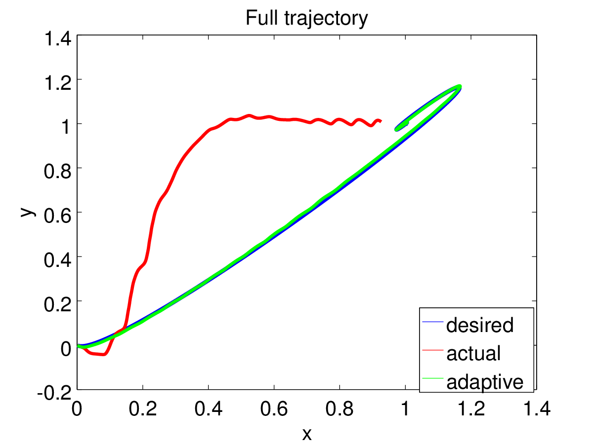
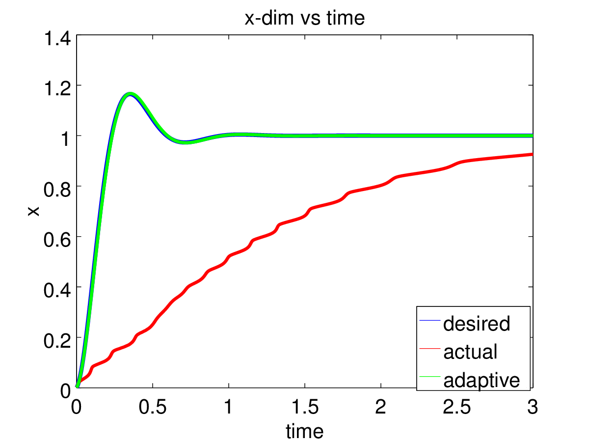
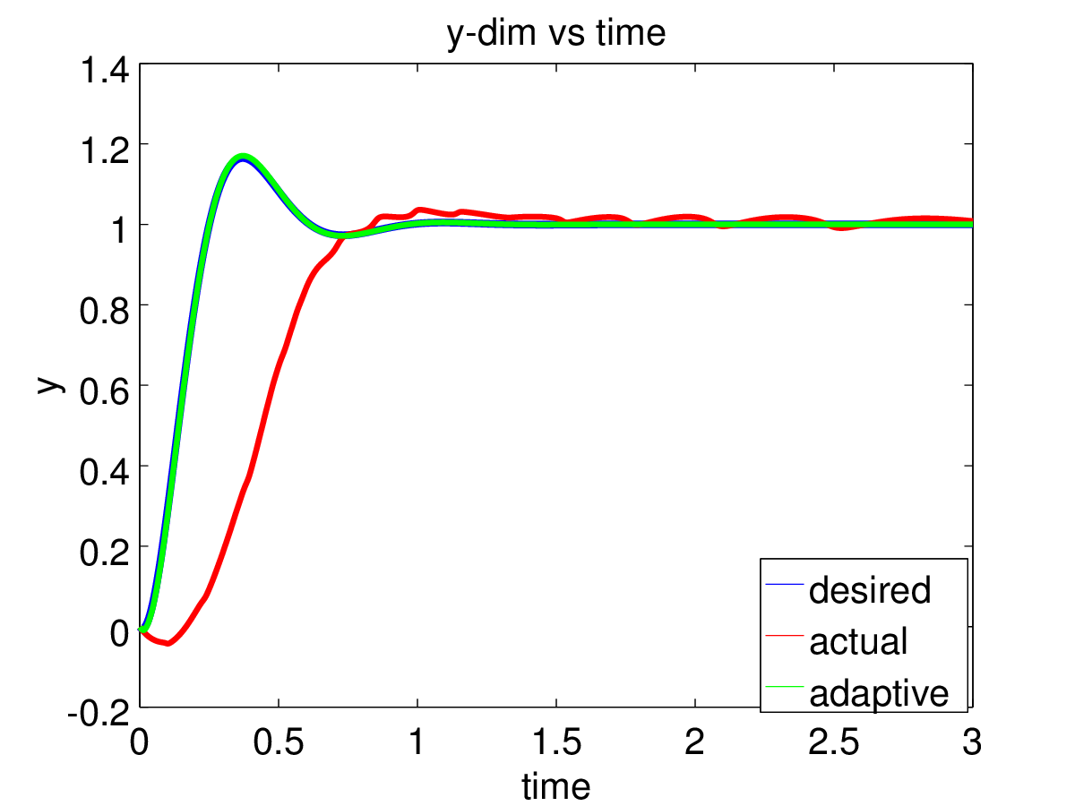
Figure 1: 2D simulation of online adaptation to severe model inaccuracies and underlying friction (which varies sinusoidally with each dimension in this case). The time axes (lower axis of the second and third plots) are in units of seconds, and all spacial axes are in units of meters. The controller updated at a rate of 1kHz.

This experiment shows a simple 2D example of the behavior of the adaptive control system for a scenario where the dynamics model used by the robot differs drastically from the true dynamics and where unmodeled nonlinear frictions are significant.

The true mass matrix of the system is defined as ${\bm{M}}({\bm{q}})=5\big{(}{\bm{v}}({\bm{q}}){\bm{v}}({\bm{q}})^{\prime}+.05{\bm{I}}\big{)}$, with ${\bm{v}}({\bm{q}})=(\sin(5q_{1});\cos(2q_{2}))$. The robot uses a diagonal constant approximation of the form $\widehat{{\bm{M}}}=.5{\bm{I}}$, which assumes masses that are an order of magnitude smaller. Additionally, the true system experiences sinusoidal frictional forces of the form

$$\mu({\bm{q}})=\left[\begin{array}[]{cc}100\sin(50\ q_{1})\\ 5\sin(50\ q_{2})\end{array}\right],$$ (31)

for which the robot has no knowledge of.

The system is using a simple PD controller (outputting accelerations) to move to a desired fixed point to a target velocity of zero.

$${\ddot{{\bm{q}}}}=K({\bm{q}}_{d}-{\bm{q}})-D{\dot{{\bm{q}}}},$$ (32)

where $K=100.$ and $D=10.$. The desired target is ${\bm{q}}_{d}=(1;1)$, and the robot starts from ${\bm{q}}_{0}=(0;0)$ with a random initial velocity.

The acceleration controller itself is tuned incorrectly and therefore overshoots. However, that’s the desired behavior we want to track (shown in blue). If we simply pipe the desired accelerations through the very approximate inverse dynamics model, the behavior we get is abysmal (shown in red). On the one hand the dynamics model is a severe approximation, and on the other hand, we have no advanced knowledge of the strange frictional pattern, so the robot drifts upward and then oscillates during the final approach. But when we turn on adaptation (shown in green), the system is able to compensate for all of that and we get very good tracking behavior.

This implementation didn’t simulate noise. But the real-world implementation discussed in the next section shows the efficacy of the above described learning tricks under noisy acceleration estimates sent back by the physical robot.

4.2 Experiments on a simulated Baxter platform

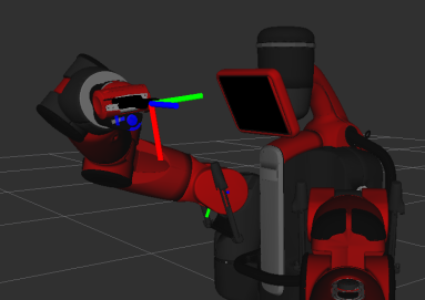
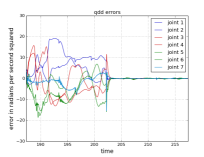
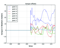
Figure 2: Left: The Baxter robot. The middle and right plots depict the acceleration errors and learned torque offsets of a 30 second run under severe nonlinear torque biasing wherein online learning was switched on half way through.

We ran a simulation experiment on the Baxter platform to analyze the performance of the online torque offset learner under severe modeling mismatches. The controller used inverse dynamics, but the simulator added substantial positionally dependent nonlinear friction and torque biases of the form

$$\tau_{\mathrm{friction}}=-7\sin^{2}(5{\bm{q}})\Big{(}2\sigma({\dot{{\bm{q}}}})-1\Big{)}\ \ \ \ \ \ \tau_{\mathrm{bias}}=-5\sin(5{\bm{q}}),$$

where $\sigma$ is the typical 0-1 sigmoidal squashing function. Additionally, the robot’s internal model did not account for joint damping coefficients, while the simulator did. The controller ran with a control cycle of $.005s$, and the simulator ran with an update cycle time of $.001s$. We ran the controller through a 30 second sequence of 10 chained 3 second Linear Quadratic Regulators (LQRs), and turned on the online learning only half way through. Figure 2 shows severe acceleration errors resulting from the model mismatch during the first half, but half way through, the online learning turns on and is able to track the torque offsets quite well, effectively zeroing the acceleration errors. The simulator added noise of the form $.001\mathrm{uniform(-1,1)}$ to both the positions and offsets when reporting them to the controller, so the raw acceleration measurements were quite noisy. The acceleration errors in the middle plot of the figure were, therefore, exponentially smoothed with a smoothing factor of $.975$. The online learner used momentum updates, which is effectively a form of smoothing, so the final plot shows the raw unsmoothed learned torque offsets used by the controller.

Note, that we have performed similar experiments both in our 2D simulated inverse dynamics setup and on our KUKA lightweight arm, which all conclusively confirm the effectiveness of the direct online learning approach.

4.3 Real-world experiments on a KUKA lightweight arm

We have a full implementation of this algorithm working for the Apollo platform (see Figure 3 (left)) for both simple Cartesian space controllers and for a full continuous optimization (MPC-type) motion generation system. The low level controller consists of an inverse dynamics controller, that evaluates the (approximate) rigid body dynamics model for desired accelerations. This inverse dynamics torque command is combined with the offset estimated by the adaptive controller, see Figure 3. In all our experiments presented here, we model the offset as a simple constant ${\bm{f}}_{\text{offset}}({\bm{q}},{\dot{{\bm{q}}}},{\ddot{{\bm{q}}}}_{d},{\bm{w}})={\bm{w}}$. The KUKA lightweight arm has $7$ degrees of freedom, thus the offset torque is a $7$-dimensional vector.

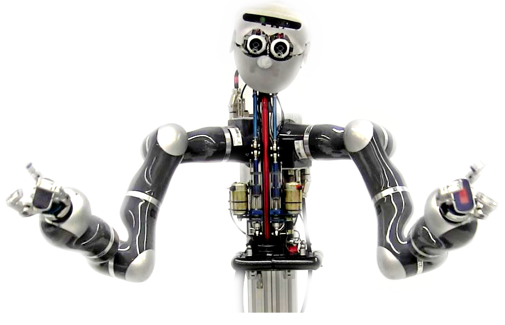
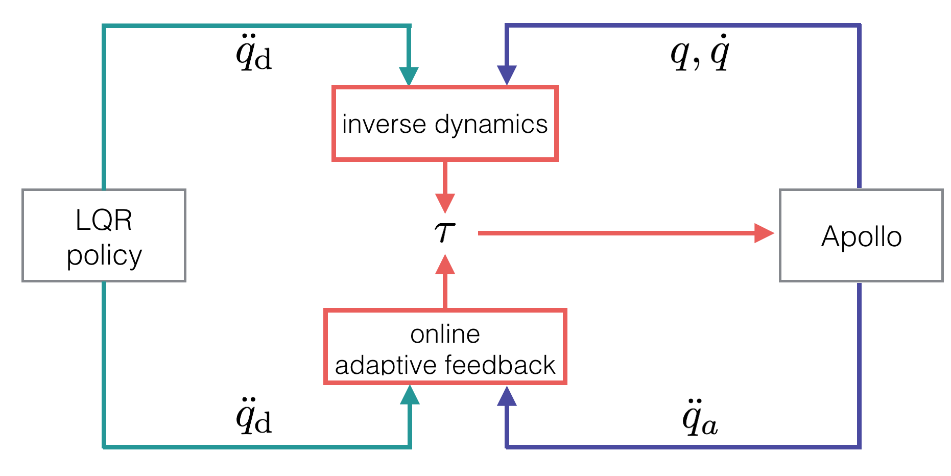
Figure 3: (left) Apollo: our experimental platform with two KUKA lightweight arms. (right) The controller used for our experiments at a rate of 1kHz.

To be robust against noise, the adaptive controller transforms the gradient ${\ddot{{\bm{q}}}}_{d}-{\ddot{{\bm{q}}}}_{a}$ as discussed in Section 3. The key parameters that are involved for the offset update are

• the learning rate $\eta$ (Equation 23),

• the variance gain $\alpha$ (Equation 28) and

• the smoothing parameter $\gamma$ (Equation 27)

These parameters are shared across all joints. We start out with analyzing the sensitivity of our proposed approach on the real Apollo platform.

4.3.1 Parameter Sensitivity Analysis

For our parameter sensitivity analysis we attempt to execute a sequence of two pre-planned LQRs. This sequence has been executed three times for each parameter combination. The considered values are:

• $\eta=0.01,0.02,\dots,0.1$

• $\alpha=0.0,0.1,\dots,0.5$

• $\gamma=0.9,0.95$

We have tested all combinations of these parameter settings and report the average acceleration error per joint for both LQRs (averaged over the three trials). If one LQR execution resulted in a unsuccessful execution (within any of the 3 trials), that parameter setting was classified as unsuccessful. We evaluate the performance and sensitivity of our approach with the help of three quantities:

The mean absolute acceleration error

between the desired and actual accelerations, $\sum_{t}|{\ddot{{\bm{q}}}}^{t}_{d}-{\ddot{{\bm{q}}}}^{t}_{a}|/T$, where T is the length of the movement. We plot this error as a function of the learning rate $\eta$ and the variance gain $\gamma$. This plot is color coded dark green to dark red. dark green indicates a very low error, dark red higher errors.

The mean acceleration error

$\sum_{t}({\ddot{{\bm{q}}}}^{t}_{d}-{\ddot{{\bm{q}}}}^{t}_{a})/T$. A value of $0$ here would mean on average the actual accelerations are neither under nor over the desired acceleration. This plot is color coded from red to blue. Red means, on average, we measure actual accelerations over the desired, blue means we measure actual accelerations below the desireds. Darker colors indicate a higher bias. Yellow colors represent a bias close $0$.

The mean absolute magnitude

of the adaptive torque command computed $\sum_{t}{\bm{f}}_{\text{offset}}^{t}/T$. The magnitude of torque offset the adaptive controller adds to the torque command. Darker color indicates larger magnitudes.

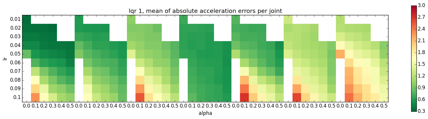
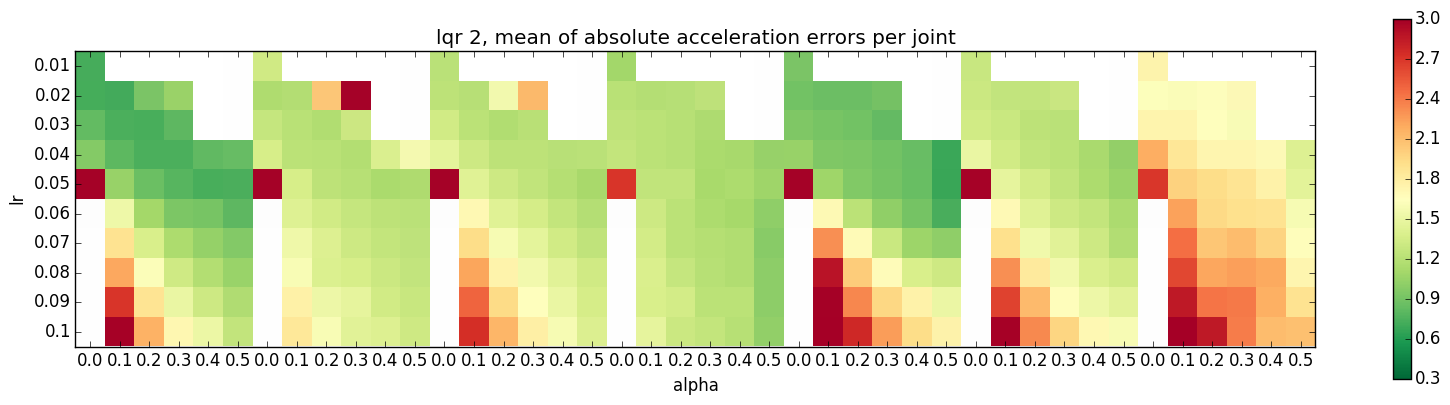
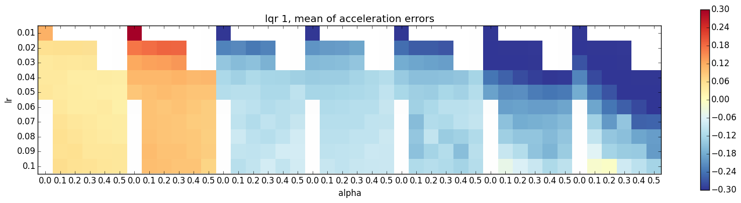
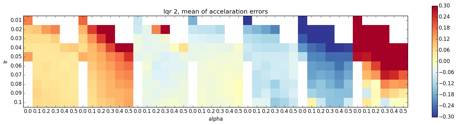
Figure 4: The average acceleration error and the error bias for both LQRs with $\gamma=0.9$. Results are displayed per joint, from left to right joint 1 to 7. From top to bottom: the average absolute acceleration for LQR #1 and #2, the mean of the acceleration error bias for both LQRs.

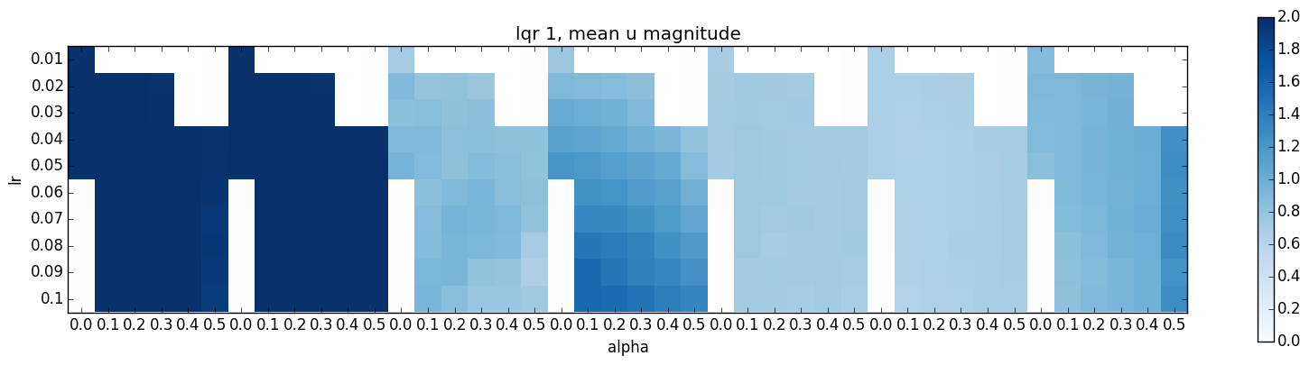
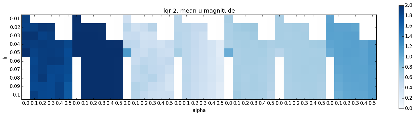
Figure 5: Torque magnitudes estimated by the adaptive controller $\gamma=0.9$. (top) LQR #1, (bottom) LQR #2. Results are shown per joint, from left to right joint 1 to 7.

In Figure 4 we plot the average absolute acceleration error and the bias of the acceleration error, for all combinations of $\eta$ and $\alpha$ while keeping $\gamma=0.9$ fixed. The first result to notice is that we were able to run the controller for a large portion of parameter combinations. While the error varies across the parameter settings, we can deduce that even without an additional error feedback term, we don’t have to perform excessive tuning of the parameters to obtain an (empirically) well behaved controller. Note, that in all failure cases (indicated by white squares in the plots) it was typically during the execution of the 2nd LQR that the movement was deemed unsafe.

The second result is that there seems to exist a relative large band across the 2 parameter settings that seems to achieve low acceleration errors (top two plots of Figure 4). This promises that tuning the adaptive controller is not too difficult.

When looking at the mean acceleration error bias we notice that we seem to typically overestimate the required torques for joints $1$ and $2$ (the shoulder joints) and underestimate the required torque for joints $3-6$. This is best understood, by keeping in mind that we are fixing the approximate RBD model. Depending on the movement this approximate model may over or underestimate the required torque to achieve desired accelerations. If the adaptive controller can fix the model - the bias should become smaller (which is represented by lighter colors). For low learning rates, we tend to observe larger bias values, This indicates that we may not be adapting to the error fast enough, and we consistently over/underestimate the required torque offsets, as can be seen in Figure 4, for joints 2-4 for instance.

However, simply increasing the learning rate is not necessarily the right thing to do. Notice, although for joint 1 we observe a small bias of the acceleration error for higher learning rates, the average absolute error increases as we increase the learning rate. This tells us that there may be oscillations, that on average have a small bias. This can mean that we are too aggressive in trying to fix the model, incurring larger acceleration errors, that we try to account for at the next time step. The severity this effect seems to also be a function of the variance gain. With smaller values this effect seems to pronounced (for instance, see joint 1, LQR # 2 the bottom left corner for both error measures).

Finally, to make sure that our adaptive torque offset estimates are sensible, we plot the offset torque magnitude per joint in Figure 5. We observe, that for the should joints we estimate higher torque offsets than for the the elbow and wrist joints. In general the offset torques range between $0Nm$ to $2Nm$, which is a reasonable range.

We have repeated the same set of experiments with a smoothing parameter of $\gamma=0.95$. The figures for this set of experiments can be found in the appendix A. In general, the relationship between the variance gain and learning rate is similar to the above presented results. However, we notice that the the effect of higher learning rates is more extreme for some joints. For instance, for joint 5, the acceleration error seems to increase faster (as the learning rate is increased), indicating that oscillations are a function of both the learning rate and smoothing parameter. Intuitively, this makes sense, as the smoothing slows down the response to the errors as well, thus a high learning rate with a very little smoothing seem to not be an optimal pairing.

All in all we can conclude that the adaptive controller can effectively fix errors in the dynamics model on the fly. Tuning the parameters, while unavoidable, is not too difficult.

4.3.2 Video demonstrations

The following three videos show examples of the dynamics adaptation algorithm running on the Apollo manipulation platform. In the first two videos, Apollo is directly executing an acceleration policy designed to generate Cartesian motion moving his finger to a fixed point in space. In the final video, Apollo is executing optimized grasping behaviors.

1. Robustness to perturbation: https://youtu.be/clldz75ToVI
   In this video, Apollo is repeatedly perturbed away from the fixed point and allowed to return under the control of the acceleration policy. The behavior is shaped by the desired accelerations, which Apollo is able to accurately reproduce by running the online learning adaptive control method outlined above to track how the dynamics model error shifts throughout the execution.

2. Bounce tests: https://youtu.be/m0i5oHQeqA8
   In this video, Apollo is put through a series of more aggressive bounce tests in an attempt to incite oscillation modes. The robustness measures outlined above successfully combat the maneuvers and Apollo’s behavior remains natural throughout the attempt.

3. Grasp tasks: https://youtu.be/LQABeK2IO80
   In this video, Apollo is executing grasp task motions optimized on on the fly. Each motion is sent down to control as a sequence of affine acceleration policies which are directly executed using the online learning adaptive control methodology described in this document. No vision is used; the sequence of object locations is planned out in advance. The system, however, uses force control in the grasps (reading from the fingertip’s strain gauges) to be robust to variations in size and specific positioning of the objects.

The underlying adaptive control parameterization is the same in all cases—we tune once and that enables the execution of any number of acceleration policies.

5 Theoretical connections and notes

This section presents some additional theoretical results to give the direct loss adaptive control methods discussed in this paper context. We start by using the techniques from above to derive a related loss function whose constant step size online gradient descent is PID control. This analysis shows that we can additionally reinterpret classical algorithms as forms of online gradient descent on concrete loss functions, and that we can potentially leverage these techniques to generalize PID control to be more adaptive by utilizing modern tools from the machine learning literature.

We also present a result that addresses some of the questions around why we can use finite-differenced accelerations in practice, despite their noise. We show that gradient descent on the acceleration loss presented above (the simplest constant step size variant) can be viewed as a form of virtual velocity control—by expanding the terms of the algorithm and rearranging them, the finite-differenced accelerations, to a large extent, telescope into a nice compact virtual velocity estimate over time. Despite the high variance of the finite-differenced acceleration estimates themselves, the final expression collapses into a form dependent on just velocity measurements (which are either directly measurable or at most first-order differenced), showing that the variance of the control law itself is actually much lower than would be expected from a simple additive noise argument under finite-differenced accelerations.

5.1 A loss function for PID control

In much of this paper, we have assumed that the robot is following a feedback acceleration policy producing a steady stream of (only) desired accelerations as a function of state ${\ddot{{\bm{q}}}}_{d}={\bm{f}}({\bm{q}},{\dot{{\bm{q}}}})$. In this section, we show how we can leverage similar ideas to write out related objective terms measuring errors in position and velocity as well. We’ll see that one particular variant of the resulting online learning algorithm is the traditional PID control used frequently in many real-world systems.

We’ve already seen in Section 3 an online learning algorithm for directly minimizing acceleration errors given desired acceleration signals ${\ddot{{\bm{q}}}}_{d}$. This section derives similar objective terms that measure the error relative to desired position ${\bm{q}}_{d}$ and velocity ${\dot{{\bm{q}}}}_{d}$ signals as well.

5.1.1 Position error term

Executing an acceleration ${\ddot{{\bm{q}}}}_{a}^{t}({\bm{w}})$ for $\Delta t$ seconds from ${\bm{q}}$ (moving at velocity ${\dot{{\bm{q}}}}$) results in a new position given by

$${\bm{q}}_{a}^{t+1}({\bm{w}})={\bm{q}}^{t}+\Delta t\ {\dot{{\bm{q}}}}^{t}+\frac{1}{2}\Delta t^{2}{\ddot{{\bm{q}}}}_{a}^{t}({\bm{w}}).$$ (33)

If we desire to be at ${\bm{q}}_{d}^{t+1}$ after executing an actual measured acceleration ${\ddot{{\bm{q}}}}_{a}^{t}({\bm{w}})$ from the current state, the resulting position error can, therefore, be expressed as

$$l_{\textrm{pos}}^{t+1}({\bm{w}})=\frac{1}{\Delta t^{2}}\|{\bm{q}}_{d}^{t+1}-{\bm{q}}_{a}^{t+1}({\bm{w}})\|_{{\bm{M}}_{t}}^{2},$$ (34)

where ${\bm{M}}_{t}$ is the true mass matrix which defines the real system dynamics at the time of executing the acceleration. The derivative is

$$\nabla_{\bm{w}}l_{\mathrm{pos}}^{t+1}({\bm{w}}) =-\frac{2}{\Delta t^{2}}\left[\frac{\partial{\bm{q}}_{a}^{t+1}({\bm{w}})}{\partial{\bm{w}}}\right]^{T}{\bm{M}}_{t}\Big{(}{\bm{q}}_{d}^{t+1}-{\bm{q}}_{a}^{t+1}({\bm{w}})\Big{)}$$ (35)

$$=-{\bm{J}}_{f_{t}}^{T}\Big{(}{\bm{q}}_{d}^{t+1}-{\bm{q}}_{a}^{t+1}({\bm{w}})\Big{)},$$ (36)

since $\frac{\partial{\bm{q}}_{a}^{t+1}({\bm{w}})}{\partial{\bm{w}}}=\frac{1}{2}\Delta t^{2}{\bm{M}}_{t}^{-1}{\bm{J}}_{f_{t}}$. This gradient is the position error pushed through the Jacobian.

5.1.2 Velocity error term

Similarly, executing acceleration ${\ddot{{\bm{q}}}}_{a}^{t}({\bm{w}})$ for $\Delta t$ seconds from velocity ${\dot{{\bm{q}}}}^{t}$ results in a new velocity given by

$${\dot{{\bm{q}}}}_{a}^{t+1}({\bm{w}})={\dot{{\bm{q}}}}^{t}+\Delta t\ {\ddot{{\bm{q}}}}_{a}^{t}({\bm{w}}).$$ (37)

If we desire to be at velocity ${\dot{{\bm{q}}}}_{d}^{t+1}$ after executing an actual measured acceleration ${\ddot{{\bm{q}}}}_{a}^{t}({\bm{w}})$ from the current state, the resulting velocity error can, therefore, be expressed as

$$l_{\textrm{vel}}^{t+1}({\bm{w}})=\frac{1}{2\Delta t}\|{\dot{{\bm{q}}}}_{d}^{t+1}-{\dot{{\bm{q}}}}_{a}^{t+1}({\bm{w}})\|_{{\bm{M}}_{t}}^{2},$$ (38)

where again ${\bm{M}}_{t}$ is the true mass matrix which defines the real system dynamics at the time of executing the acceleration. The derivative is

$$\nabla_{\bm{w}}l_{\mathrm{vel}}^{t+1}({\bm{w}}) =-\frac{1}{\Delta t}\left[\frac{\partial{\bm{q}}_{a}^{t+1}({\bm{w}})}{\partial{\bm{w}}}\right]^{T}{\bm{M}}_{t}\Big{(}{\dot{{\bm{q}}}}_{d}^{t+1}-{\dot{{\bm{q}}}}_{a}^{t+1}({\bm{w}})\Big{)}$$ (39)

$$=-{\bm{J}}_{f_{t}}^{T}\Big{(}{\dot{{\bm{q}}}}_{d}^{t+1}-{\dot{{\bm{q}}}}_{a}^{t+1}({\bm{w}})\Big{)},$$ (40)

since $\frac{\partial{\bm{q}}_{a}^{t+1}({\bm{w}})}{\partial{\bm{w}}}=\Delta t{\bm{M}}^{-1}_{t}{\bm{J}}_{f_{t}}$. This gradient is the velocity error pushed through the Jacobian.

5.1.3 The PID objective

Combining these two terms with the acceleration error term derived in Section 3, gives an objective of the form

$$l^{t}({\bm{w}}) =\alpha\ l_{\mathrm{pos}}^{t}({\bm{w}})+\beta\ l_{\mathrm{vel}}^{t}({\bm{w}})+\gamma\ l_{\mathrm{acc}}^{t}({\bm{w}})$$ (41)

$$=\frac{\alpha}{\Delta t^{2}}\|{\bm{q}}_{d}^{t}-{\bm{q}}_{a}^{t}({\bm{w}})\|_{{\bm{M}}_{t}}^{2}+\frac{\beta}{2\Delta t}\|{\dot{{\bm{q}}}}_{d}^{t}-{\dot{{\bm{q}}}}_{a}^{t}({\bm{w}})\|_{{\bm{M}}_{t}}^{2}+\frac{\gamma}{2}\|{\ddot{{\bm{q}}}}_{d}^{t}-{\ddot{{\bm{q}}}}_{a}^{t}({\bm{w}})\|_{{\bm{M}}_{t}}^{2},$$ (42)

where $\alpha$, $\beta$, and $\gamma$ are scaling constants. The gradient is given by

$$\nabla_{{\bm{w}}}l^{t}({\bm{w}}_{t})=-{\bm{J}}^{T}_{f_{t-1}}\Big{(}\alpha\left({\bm{q}}_{d}^{t}-{\bm{q}}_{a}^{t}\right)+\beta\left({\dot{{\bm{q}}}}_{d}^{t}-{\dot{{\bm{q}}}}_{a}^{1}\right)\Big{)}+\gamma{\bm{J}}^{T}_{f}\left({\ddot{{\bm{q}}}}_{d}^{t}-{\ddot{{\bm{q}}}}_{a}^{t}\right),$$ (43)

where ${\bm{J}}_{f_{t}}$ is the Jacobian of the offset function at ${\bm{w}}_{t}$.

A number of gradient-based algorithms can be derived from this gradient expression. But in particular, consider ${\bm{f}}_{\text{offset}}({\bm{w}})={\bm{w}}$ such that ${\bm{J}}_{f_{t}}={\bm{I}}$ for all $t$. Then summing these gradients under a constant step size of $\Delta t$, which implements a vanilla constant step size gradient descent method, results in the following control law:

$${\bm{w}}^{t} ={\bm{\tau}}^{t}=-\sum_{\kappa=0}^{t-1}\nabla_{\bm{w}}l^{\kappa}({\bm{w}}^{\kappa})$$ (44)

$$=\alpha\sum_{\kappa=0}^{t-1}\left({\bm{q}}^{\kappa}_{d}-{\bm{q}}^{\kappa}_{a}\right)\Delta t+\beta\sum_{\kappa=0}^{t-1}\left({\dot{{\bm{q}}}}^{\kappa}_{d}-{\dot{{\bm{q}}}}^{\kappa}_{a}\right)\Delta t+\gamma\sum_{\kappa=0}^{t-1}\left({\ddot{{\bm{q}}}}^{\kappa}_{d}-{\ddot{{\bm{q}}}}^{\kappa}_{a}\right)\Delta t$$ (45)

$$=\alpha\sum_{\kappa=0}^{t-1}\left({\bm{q}}^{\kappa}_{d}-{\bm{q}}^{\kappa}_{a}\right)\Delta t+\beta\left({\bm{q}}^{t}_{d}-{\bm{q}}^{t}_{a}\right)+\gamma\left({\dot{{\bm{q}}}}^{t}_{d}-{\dot{{\bm{q}}}}^{t}_{a}\right).$$ (46)

These three terms are the integral, position error, and velocity error terms, respectively, of a PID controller. This shows that we may view PID control as gradient descent on the objective given by 41 under a constant step size. Beyond that, it additionally shows that there is also a much broader class of learning algorithms we can leverage to achieve higher fidelity tracking as we’ve seen above in our experiments on the acceleration error term alone. Studying this broader class of PID-related algorithms is an interesting avenue for future work.

5.2 Telescoping finite-differenced accelerations: a virtual velocity control interpretation

In this section, we show that the simplest version of our algorithm, with a bit a rearranging, can be written as a form of virtual velocity control. The finite-differenced accelerations, which are worrisome to many due to possible estimation noise, telescope in the sum across time into a relatively simple form of velocity control expression wherein target velocities are integrated forward from desired accelerations (with a forgetting factor) and control signals are derived as velocity differences. We present this result first in equation form and discuss its implications, and then derive it algebraically.

5.2.1 Basic result

The simplest version gradient descent algorithm given in Equation 23, using a constant step size, takes the form:

$${\bm{\tau}}^{t+1}=\alpha({\ddot{{\bm{q}}}}_{d}^{t}-{\ddot{{\bm{q}}}}_{a}^{t})+(1-\alpha\widetilde{\lambda}){\bm{\tau}}^{t},$$ (47)

where $\alpha$ is the constant step size and $\widetilde{\lambda}$ is the regularization constant. This algorithm is gradient descent using gradient $-({\ddot{{\bm{q}}}}_{d}^{t}-{\ddot{{\bm{q}}}}_{a}^{t})+\widetilde{\lambda}{\bm{\tau}}^{t}$. For the analysis below, it’s convenient to define $\alpha\widetilde{\lambda}=1-\lambda$ so that the result is more comparable to the next algorithm, which is why we use a slightly different notation here than in Equation 23.

We will show below that if we expand this recursive relationship and rearrange some terms, we can write this (constant step size) control law as the form

$${\bm{\tau}}^{t+1}=\alpha\Big{[}\Big{(}\underbrace{\big{(}\lambda{\bm{v}}^{t}+(1-\lambda){\dot{{\bm{q}}}}^{t}\big{)}+\Delta t{\ddot{{\bm{q}}}}_{d}^{t}}_{{\bm{v}}^{t+1}}\Big{)}-{\dot{{\bm{q}}}}^{t}\Big{]}.$$ (48)

Here ${\bm{v}}^{t}$ is a virtual target velocity vector that’s integrated forward using the desired accelerations. At the beginning of each control cycle the virtual velocity vector is blended slightly with the current state via a forgetting factor and then integrated forward by one step using the desired acceleration ${\ddot{{\bm{q}}}}_{d}^{t}$.

In all cases, ${\ddot{{\bm{q}}}}_{d}^{t}={\bm{f}}({\bm{q}}^{t},{\dot{{\bm{q}}}}^{t})$ is the desired acceleration evaluated at the current measured state.

5.2.2 Discussion

In general, leveraging finite-differenced accelerations is worrisome due to the noise in the estimates. We’ve shown experimentally, however, that it can work in practice for this particular algorithm, enabling accurate tracking of raw acceleration policies. The result in Section 5.2.1 provides some insight into why.

At a high level, since we’re summing across finite-differenced acceleration errors over time, we’re effectively integrating. The sum of true accelerations becomes the true velocity and the sum of desired accelerations becomes a virtual desired velocity (there are some details regarding the forgetting factor (see the next section), but this is the basic mechanism at work). This algorithm is, therefore, a form of velocity control where desired velocities are generated from the underlying acceleration policy. In practice, we use more sophisticated variants of gradient-based online learning that leverage varying step sizes, momentum, or other tricks that offer increased adaptation in real time. The basic structure of these algorithms is the same, and the overall numerical process retains the same sort of telescoping form making it suitable for practical execution.

5.2.3 Equivalence

This section derives the equivalence result discussed in Section 5.2.1. We can show the equivalence by expanding the rules and writing them both as a difference between a virtual desired velocity and the current velocity. We start with the online learning variant.

Direct loss adaptive control algorithm expansion

Using the notation $\alpha\widetilde{\lambda}=1-\lambda$, we can rewrite the online learning rule in Equation 47 as

$${\bm{\tau}}^{t+1} =\alpha({\ddot{{\bm{q}}}}_{d}^{t}-{\ddot{{\bm{q}}}}_{a}^{t})+\lambda{\bm{\tau}}^{t}$$ (49)

$$=\alpha\Big{(}\big{(}{\ddot{{\bm{q}}}}_{d}^{t}-{\ddot{{\bm{q}}}}_{a}^{t}\big{)}+\lambda\big{(}{\ddot{{\bm{q}}}}_{d}^{t-1}-{\ddot{{\bm{q}}}}_{a}^{t-1}\big{)}+\cdots\Big{)}.$$ (50)

We see here that $\alpha$ is just a gain, so we can drop it without loss of generality. Now we expand the acceleration estimate in terms of its finite-differencing expression ${\ddot{{\bm{q}}}}^{t}=\frac{1}{\Delta t}\big{(}{\dot{{\bm{q}}}}^{t}-{\dot{{\bm{q}}}}^{t-1}\big{)}$:

$${\bm{\tau}}^{t+1} \propto\Big{(}{\ddot{{\bm{q}}}}_{d}^{t}-\frac{1}{\Delta t}\big{(}{\dot{{\bm{q}}}}^{t}-{\dot{{\bm{q}}}}^{t-1}\big{)}\Big{)}+\lambda\Big{(}{\ddot{{\bm{q}}}}_{d}^{t-1}-\frac{1}{\Delta t}\big{(}{\dot{{\bm{q}}}}^{t-1}-{\dot{{\bm{q}}}}^{t-2}\big{)}\Big{)}+\cdots$$ (51)

The key observation is that we almost have a telescoping sum in these finite-differencing terms. If $\lambda$ were $1$, the sum would telescope and result in just $-\frac{1}{\Delta t}{\dot{{\bm{q}}}}^{t}$. Instead, we get some (significant) residual from those terms and it’s insightful to group them together:

$${\bm{\tau}}^{t+1}\ \ \propto\ \ {\ddot{{\bm{q}}}}_{d}^{t}+\lambda{\ddot{{\bm{q}}}}_{d}^{t-1}+\lambda^{2}{\ddot{{\bm{q}}}}_{d}^{t-2}+\cdots$$ (52)

$$-\frac{1}{\Delta t}{\dot{{\bm{q}}}}^{t}$$ (53)

$$+\underbrace{\left(\frac{1}{\Delta t}{\dot{{\bm{q}}}}^{t-1}-\frac{\lambda}{\Delta t}{\dot{{\bm{q}}}}^{t-1}\right)+\left(\frac{\lambda}{\Delta t}{\dot{{\bm{q}}}}^{t-2}-\frac{\lambda^{2}}{\Delta t}{\dot{{\bm{q}}}}^{t-2}\right)+\cdots.}_{\frac{1-\lambda}{\Delta t}\Big{(}{\dot{{\bm{q}}}}^{t-1}+\lambda{\dot{{\bm{q}}}}^{t-2}+\cdots\Big{)}}$$ (54)

Collapsing these terms into summation expressions and pulling out the $1/\Delta t$ as a constant factor (and absorbing it into the proportionality), we get

$${\bm{\tau}}^{t+1}\ \ \propto\ \ \sum_{\kappa=0}^{t}\lambda^{\kappa}\Delta t{\ddot{{\bm{q}}}}_{d}^{t-\kappa}-{\dot{{\bm{q}}}}^{t}+(1-\lambda)\sum_{\kappa=0}^{t-1}\lambda^{\kappa}{\dot{{\bm{q}}}}^{t-\kappa-1}.$$ (55)

Note that $\sum_{\kappa=0}^{\infty}\lambda^{\kappa}=\frac{1}{1-\lambda}$. Thus, as $t$ gets larger, $1-\lambda$ increasingly approximates a normalization factor on weights $\lambda^{\kappa}$. So defining $w^{\kappa}=(1-\lambda)\lambda^{\kappa}$, it’s increasingly accurate to say $\sum_{\kappa=0}^{t}=w^{\kappa}\approx 1$, i.e. using the weights in a sum forms a exponential weighted average. Using this notation, and rearranging the terms slightly, we get

$${\bm{\tau}}^{t+1}\ \ \propto\ \ \underbrace{\Big{(}\sum_{\kappa=0}^{t-1}w^{\kappa}{\dot{{\bm{q}}}}^{t-\kappa-1}+\sum_{\kappa=0}^{t}\lambda^{\kappa}\Delta t{\ddot{{\bm{q}}}}_{d}^{t-\kappa}}_{\widetilde{{\bm{v}}}^{t+1}}\Big{)}-{\dot{{\bm{q}}}}^{t}.$$ (56)

We explicitly attribute the first two terms to the virtual velocity $\widetilde{{\bm{v}}}^{t+1}$. The intuition is that the first term $\sum_{\kappa}w^{\kappa}{\dot{{\bm{q}}}}^{t-\kappa-1}$ is just a smoothed estimate of the velocity found by calculating a exponentially decaying weighted average over the measured velocities. The second term $\sum_{\kappa}\lambda^{\kappa}\Delta t{\ddot{{\bm{q}}}}_{d}^{t-\kappa}$, on the other hand, is a vector defining (approximately) what velocity we should have gotten if we actually accelerated from $0$ as defined by the sequence of desired accelerations ${\ddot{{\bm{q}}}}_{d}^{t-\kappa}$. Each $\Delta t{\ddot{{\bm{q}}}}_{d}^{t-\kappa}$ is what we’d add to the velocity in an integration step. If $\lambda=1$, this expression would exactly be the integration expression. But since $\lambda<1$, we actually have it fully using the first term $\Delta t{\ddot{{\bm{q}}}}_{d}^{t}$ accounting for the latest acceleration, but increasingly forgetting past accelerations over time. That first sum expresses the velocity we should see starting from zero, so adding it to the weighted average velocity defines where we actually end up starting from the (smoothed) measured velocity. That smoothed measured velocity is constantly updating to the robot’s current velocity, and the acceleration integration term is forgetting old accelerations at the same rate (with exponential decay), so the combined process stays up-to-date at complimentary rates.

This analysis shows that we can view the online gradient descent algorithm as a form of virtual velocity feedback control with a virtual velocity vector of the form:

$$\widetilde{{\bm{v}}}^{t+1}=\sum_{\kappa=0}^{t-1}w^{\kappa}{\dot{{\bm{q}}}}^{t-\kappa-1}+\sum_{\kappa=0}^{t}\lambda^{\kappa}\Delta t{\ddot{{\bm{q}}}}_{d}^{t-\kappa}$$ (57)

The next subsection shows that this is essentially the same expression as is used by the classical algorithm.

Virtual velocity feedback expansion

Now lets expand the virtual velocity expression in the classical update rule of Equation 48:

$${\bm{v}}^{t+1} =\Big{[}\lambda{\bm{v}}^{t}+(1-\lambda){\dot{{\bm{q}}}}^{t}\Big{]}+\Delta t{\ddot{{\bm{q}}}}_{d}^{t}$$ (58)

$$=\Big{[}\lambda\Big{(}\lambda{\bm{v}}^{t-1}+(1-\lambda){\dot{{\bm{q}}}}^{t-1}+\Delta t{\ddot{{\bm{q}}}}_{d}^{t-1}\Big{)}+(1-\lambda){\dot{{\bm{q}}}}^{t}\Big{]}+\Delta t{\ddot{{\bm{q}}}}_{d}^{t}$$ (59)

$$=\lambda^{2}{\bm{v}}^{t-1}+\lambda(1-\lambda){\dot{{\bm{q}}}}^{t-1}+(1-\lambda){\dot{{\bm{q}}}}^{t}+\lambda\Delta t{\ddot{{\bm{q}}}}_{d}^{t-1}+\Delta t{\ddot{{\bm{q}}}}_{d}^{t}$$ (60)

$$=(1-\lambda)\sum_{\kappa=0}^{t}\lambda^{\kappa}{\dot{{\bm{q}}}}^{t-\kappa}+\sum_{\kappa=0}^{t}\lambda^{\kappa}\Delta t{\ddot{{\bm{q}}}}_{d}^{t-\kappa}.$$ (61)

Again, we can write $w^{\kappa}=(1-\lambda)\lambda^{\kappa}$ to get

$${\bm{v}}^{t+1}=\sum_{\kappa=0}^{t}w^{\kappa}{\dot{{\bm{q}}}}^{t-\kappa}+\sum_{\kappa=0}^{t}\lambda^{\kappa}\Delta t{\ddot{{\bm{q}}}}_{d}^{t-\kappa}.$$ (62)

Comparing this expression to that for the virtual velocity of the online learning update rule in Equation 57, we see that the two virtual velocities are essentially equivalent. The only difference is that the online learning rule uses the weighted average velocity estimate from the previous time step and the classical rule uses the estimate from this time step. Given the typical decay time scale of $\lambda$ (which often decays to zero on the order of tenths of a second) compared to the time scale of $\Delta t$ (on the order of a millisecond), the difference is negligible.

We can therefore say that the online learning rule, and the classical rule, are the effectively the same for this simple case. Using the online learning formulation, though, makes it easier to leverage more adaptive techniques from machine learning as discussed in Section 5.2.2.

6 Conclusion and Future Work

In this work, we presented a novel approach to online learning of inverse dynamics modeling errors. Our algorithm directly minimizes a loss function that directly penalizes the error between desired and actual accelerations, enabling the direct execution of raw acceleration policies such as operational space controllers and Linear Quadratic Regulator (LQR) controllers outputting desired accelerations as a function of the robot’s state. Using a direct loss overcomes the off-distribution learning issue present in indirect loss approaches which prevail in existing state-of-the art inverse dynamics learning. We have shown how we can perform online gradient descent on parameters of general nonlinear function approximators to learn an error model of the dynamics. In our extensive evaluations, even with a simple constant error model, by updating and adapting it online, we show that our approach can correct inverse dynamics errors on the fly, for real-world motion generation.

Future work will investigate the use of more complex function approximators, especially friction models and body point forces and torques to compensate for tools, sensors, and other types of loads, as well as interactions between this memory-less adaptive control style learning and learning control style iteration model improvement leveraging these updates.

Appendix A More Results

More result visualizations for the parameter sensitivity analysis of Section 4.3.1.

Figure 6: Torque magnitudes estimated by the adaptive controller $\gamma=0.95$. (top) LQR #1, (bottom) LQR #2. Results are shown per joint, from left to right joint 1 to 7.

Figure 7: The average acceleration error and the error bias for both LQRs with $\gamma=0.95$. Results are displayed per joint, from left to right joint 1 to 7. From top to bottom: the average absolute acceleration for LQR #1 and #2, the mean of the acceleration error bias for both LQRs.

References

- [1] Chae H An, Christopher G Atkeson, and John M Hollerbach. Estimation of inertial parameters of rigid body links of manipulators. In 24th IEEE Conference on Decision and Control, pages 990–995, 1985.
- [2] Chae H An, Christopher G Atkeson, and John M Hollerbach. Model-based Control of a Robot Manipulator. MIT Press (MA), 1988.
- [3] Karl J. Astrom and Dr. Bjorn Wittenmark. Adaptive Control. Dover, 2nd edition, 2008.
- [4] Christopher M. Bishop. Pattern Recognition and Machine Learning. Springer, 2007.
- [5] Léon Bottou. Stochastic Learning, pages 146–168. Springer Berlin Heidelberg, Berlin, Heidelberg, 2004.
- [6] Léon Bottou, Frank E. Curtis, and Jorge Nocedal. Optimization methods for large-scale machine learning. 2016.
- [7] N. Cesa-Bianchi, A. Conconi, and C. Gentile. On the generalization ability of on-line learning algorithms. IEEE Transactions on Information Theory 50, page 2050–2057, 2004.
- [8] Nicolo Cesa-Bianchi and Gabor Lugosi. Prediction, Learning, and Games. Cambridge University Press, New York, NY, USA, 2006.
- [9] John J Craig. Introduction to robotics: mechanics and control, volume 3. Pearson Prentice Hall Upper Saddle River, 2005.
- [10] John J Craig, Ping Hsu, and S Shankar Sastry. Adaptive Control of Mechanical Manipulators. The International Journal of Robotics Research, 1987.
- [11] John Duchi, Elad Hazan, and Yoram Singer. Adaptive subgradient methods for online learning and stochastic optimization. Journal of Machine Learning Research, 12(Jul):2121–2159, 2011.
- [12] Arjan Gijsberts and Giorgio Metta. Real-time model learning using Incremental Sparse Spectrum Gaussian Process Regression. Neural Networks, 41, 2013.
- [13] Auke Jan Ijspeert, Jun Nakanishi, Heiko Hoffmann, Peter Pastor, and Stefan Schaal. Dynamical Movement Primitives: Learning Attractor Models for Motor Behaviors. Neural computation, 25, 2013.
- [14] Petros Ioannou and Jing Sun. Robust Adaptive Control. Dover Publications; First Edition, 2012.
- [15] Diederik P. Kingma and Jimmy Ba. Adam: A method for stochastic optimization. CoRR, abs/1412.6980, 2014.
- [16] Franziska Meier, Philipp Hennig, and Stefan Schaal. Incremental Local Gaussian Regression. In Advances in Neural Information Processing Systems 27. 2014.
- [17] D Nguyen-Tuong, M Seeger, and J Peters. Local gaussian process regression for real time online model learning and control. Advances in Neural Information Processing Systems, 22, 2008.
- [18] Nathan Ratliff, J. Andrew (Drew) Bagnell, and Martin Zinkevich. (online) subgradient methods for structured prediction. In Eleventh International Conference on Artificial Intelligence and Statistics (AIStats), March 2007.
- [19] L. Righetti, M. Kalakrishnan, P. Pastor, J. Binney, J. Kelly, R. Voorhies, G. Sukhatme, and S. Schaal. An autonomous manipulation system based on force control and optimization. Autonomous Robots, 2013.
- [20] Jean-Jacques E Slotine and Weiping Li. Composite adaptive control of robot manipulators. Automatica, 1989.
- [21] R. Stengel. Optimal Control and Estimation. Dover, New York, 1994.
- [22] John R. Taylor. Classical Mechanics. University Science Books, 2005.
- [23] Sethu Vijayakumar and Stefan Schaal. Locally Weighted Projection Regression: An O(n) Algorithm for Incremental Real Time Learning in High Dimensional Space. ICML, 2000.
- [24] Larry Wasserman. All of Statistics: A Concise Course in Statistical Inference. Springer Publishing Company, Incorporated, 2010.
- [25] Martin Zinkevich. Online convex programming and generalized infinitesimal gradient ascent. In Proceedings of the 20th International Conference on Machine Learning (ICML-03), pages 928–936, 2003.