The classical harmonic chain:
solution via Laplace transforms and continued fractions

Abstract

The harmonic chain is a classical many-particle system which can be solved exactly for arbitrary number of particles (at least in simple cases, such as equal masses and spring constants). A nice feature of the harmonic chain is that the final result for the displacements of the individual particles can be easily understood – therefore, this example fits well into a course of classical mechanics for undergraduates. Here we show how to calculate the displacements by solving equations of motion for the Laplace transforms $\mathcal{L}\left\{{q_{n}}\right\}\left({s}\right)$ of the displacements $q_{n}(t)$. This leads to a continued fraction representation of the Laplace transforms which can be evaluated analytically. The inverse Laplace transform of $\mathcal{L}\left\{{q_{n}}\right\}\left({s}\right)$ finally gives the displacements which generically have the form of Bessel functions. We also comment on the similarities between this approach and the Green function method for quantum many-particle systems.

I Introduction

In this paper, we present a method to calculate the time dependence of the displacements of a classical harmonic chain with the Hamiltonian

$$H=\sum_{n=0}^{N}\frac{p_{n}^{2}}{2m_{n}}+\sum_{n=0}^{N-1}\frac{1}{2}k_{n}(q_{n+1}-q_{n})^{2}\ .$$ (1)

The chain consists of $N+1$ point masses $m_{n}$ ($n=0,1,\ldots,N$), connected by springs with spring constants $k_{n}$ (see Fig. 1). The displacements $q_{n}$ in eq. (1) are defined as $q_{n}=x_{n}-na$, with $x_{n}$ the position of mass $n$ and $a$ the lattice constant. The system is in its equilibrium state for momenta $p_{n}=0$ and displacements $q_{n}=0$.

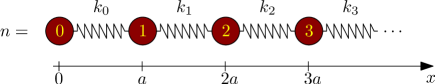
Figure 1: Sketch of the harmonic chain, corresponding to the Hamiltonian eq. (1).

To be specific, let us consider the following initial conditions: all momenta and displacements are zero except for the displacement of the oscillator at $n=0$:

$$p_{n} = 0\ ,\ n=0,1,\ldots,N\ ,$$

$$q_{0} \neq 0\ ,\ q_{n}=0\ ,\ n=1,2,\ldots,N\ .$$

Due to the coupling to the rest of the harmonic chain, the left-most oscillator ($n=0$) performs a damped oscillation as shown in Fig. 3 below (the result in Fig. 3 is calculated for the semi-infinite chain, i.e. the limit $N\to\infty$, with all $m_{n}=m$, $k_{n}=k$).

The harmonic chain is an instructive example of a classical many-particle system which can be solved exactly for any value of $N$, and it fits nicely into a classical mechanics course for 1st or 2nd year students. The standard approach is to map the Newton equations of motion, via a suitable ansatz, to a problem of linear algebra, that is the calculation of eigenvalues and eigenvectors of an $(N+1)\times(N+1)$ matrix. This can be done analytically, at least for simple cases such as equal masses and equal spring constants.

Here we pursue a different strategy which works as follows:

• As a central quantity, we work with the Laplace transform $\mathcal{L}\left\{{q_{n}}\right\}\left({s}\right)$ of the time-dependent displacements $q_{n}(t)$.

• For these Laplace transforms, we derive equations of motion which involve Poisson brackets $\{\ldots,H\}$ between the $q_{n}$ (or $p_{n}$) and the Hamiltonian $H$.

• Evaluation of these Poisson brackets gives a sequence of equations of motion which can be put into the form of a continued fraction.

• For equal masses and spring constants, and in the limit $N\to\infty$, the continued fraction can be evaluated analytically. The spectral function of the Laplace transform $\mathcal{L}\left\{{q_{0}}\right\}\left({s}\right)$ then acquires a semi-elliptic shape, see Fig. 2.

• Finally, the inverse Laplace transform gives the time-dependent function $q_{0}(t)$ which (for the special case mentioned above) has the shape of a Bessel function, see Fig. 3.

This program appears to be considerably more complex than the standard approach of mapping to an eigenvalue problem, so what is the benefit of going through all these steps? We think the main benefit here is for the students to see various concepts of analytical mechanics – and theoretical physics in general – working in an example for which the physics can be intuitively understood. Parts of the derivation such as the calculation of the Poisson brackets or the derivation of some of the properties of the Laplace transform might also be used as exercises in problem classes (while the whole strategy should certainly be explained in a lecture).

Furthermore, going through the calculation of $q_{0}(t)$ can serve as a preparation for more advanced topics of theoretical physics. As we will discuss in Sec. VII, there are close analogies between the formalism presented here and the Green function formalism for quantum many-particle systems. In fact, the calculation of the Green function for the first site of a tight-binding chain very much resembles the calculation of the Laplace transform $\mathcal{L}\left\{{q_{0}}\right\}\left({s}\right)$, and the shape of the resulting spectral function (the semi-elliptic form in Fig. 2) is identical. One of the analogies here is the correspondence between the Poisson brackets in classical mechanics and the commutators in quantum mechanics which results in equations of motion with a very similar structure.

In Secs. II, III, IV, and V we follow the steps outlined above with the final result for $q_{0}(t)$ discussed in Sec. V. The approach can be generalized to other one-dimensional geometries, such as the infinite chain discussed in Sec. VI. For this case, we show that the displacements $q_{n}(t)$ are proportional to the Bessel functions $J_{2n}\left(\sqrt{\frac{4k}{m}}t\right)$, see eq. (66), a result which might also be useful as an example of the appearance of Bessel functions in a physical system. Section VII is devoted to the analogies to the quantum case and a summary is given in Sec. VIII.

Various issues of the classical harmonic chain have, of course, been dealt with in the literature, using approaches different to the one developed here. Goodman Goodman , for example, derives the result for the displacements $q_{n}(t)$ – see eqs. (49,69) employing a normal mode expansion. The propagation of a localized impulse in a harmonic chain, a situation which is realized by the initial conditions in eq. (47), has been discussed in detail by Merchant and Brill Merchant , using a similar method. An interesting extension of our approach would be to include external time-dependent forces, which leads to interesting results as discussed in Cannas and PratoCannas . They also discussed analogies to the scattering of a quantum particle at a Kronig-Penney potential.

II Laplace transform

For a given time-dependent function $f(t)$, we define the Laplace transform $\mathcal{L}\left\{{f}\right\}\left({s}\right)$ as

$$\mathcal{L}\left\{{f}\right\}\left({s}\right)=\int_{0}^{\infty}{\rm d}t\,e^{-st}f(t)\ ,$$ (2)

with $s=\delta+i\omega$ and $\delta>0$. The functions $f(t)$ we are dealing with do not grow exponentially (or faster) with time. In this case, the Laplace transform is an analytic function in the whole right half of the complex plane.

As an example, consider the function

$$f(t)=b\,\cos(\bar{\omega}t)\ ,$$ (3)

which corresponds, in the model introduced in Sec. I, to an undamped oscillation of the displacement $q_{0}(t)$. The Laplace transform can be easily evaluated as

$$\mathcal{L}\left\{{f}\right\}\left({s}\right)=\frac{b}{2}\left[\frac{1}{s-i\bar{\omega}}+\frac{1}{s+i\bar{\omega}}\right]\ .$$ (4)

It is convenient to illustrate the Laplace transform via its spectral function defined as

$$S(\omega)=\frac{1}{\pi}\lim\limits_{\delta\rightarrow 0}\operatorname{Re}\mathcal{L}\left\{{f}\right\}\left({\delta+i\omega}\right)\ .$$ (5)

With the identity

$$\lim_{\delta\to 0}\frac{1}{\delta+ix}=-i{\cal P}\left(\frac{1}{x}\right)+\pi\delta(x)\ ,$$ (6)

(with ${\cal P}$ the principal value and $\delta(x)$ the $\delta$-function) we obtain

$$S(\omega)=\frac{b}{2}\left[\delta(\omega-\bar{\omega})+\delta(\omega+\bar{\omega})\right]\ .$$ (7)

In this case, the spectral function is discrete – a sum of two $\delta$-functions; performing the inverse Laplace transformation one can see how these two $\delta$-functions combine again to give a single oscillator mode, i.e. the $\cos$-term in eq. (3). For an infinite system, we expect an infinite number of oscillation modes; the resulting spectral function then turns out to be continuous, as in the example discussed in Sec. IV, see eq. (38).

The properties of the Laplace transform are discussed in detail in various books, see for example Ref. AbramowitzStegun, ; here is a list of some of the properties which are used in the following sections:

• Initial value and final value theorem:

  $$\lim\limits_{s\rightarrow\infty}s\mathcal{L}\left\{{f}\right\}\left({s}\right)=\lim\limits_{t\searrow 0}f(t)\ .$$ (8)

  $$\lim\limits_{s\searrow 0}s\mathcal{L}\left\{{f}\right\}\left({s}\right)=\lim\limits_{t\rightarrow\infty}f(t)\ .$$ (9)

  Both theorems are valid if the limit exists.

• Laplace transform of the integral:

  $$\frac{1}{s}\mathcal{L}\left\{{f}\right\}\left({s}\right)=\mathcal{L}\left\{{\int_{0}^{t}\textnormal{d}\tau f(\tau)}\right\}\left({s}\right)\ .$$ (10)

III equations of motion

In Hamiltonian mechanics, a classical physical system with $N$ degrees of freedom is described by a set of canonical coordinates $(q=(q_{1},\ldots,q_{N}),p=(p_{1},\ldots,p_{N}))$. The time evolution is described by Hamilton’s equations

$$\frac{\textnormal{d}p_{n}}{\textnormal{d}t}=-\frac{\partial H}{\partial q_{n}},\qquad\frac{\textnormal{d}q_{n}}{\textnormal{d}t}=\frac{\partial H}{\partial p_{n}}\ .$$ (11)

For two functions $f(p,q,t)$ and $g(p,q,t)$ on phase space, the Poisson-bracket is defined as

$$\left\{f,g\right\}=\sum\limits_{n=1}^{N}\left[\frac{\partial f}{\partial q_{n}}\frac{\partial g}{\partial p_{n}}-\frac{\partial f}{\partial p_{n}}\frac{\partial g}{\partial q_{n}}\right]\ .$$ (12)

¿From Hamilton’s equations (11) one obtains equations of motion for the total time derivative of a function $f(q,p,t)$

$$\dot{f}=Lf+\frac{\partial f}{\partial t}\ ,$$ (13)

where $L:=\left\{.,H\right\}$ is the Liouville operator and $\dot{f}$ denotes the total time derivative of $f$. Consider now

$$\frac{\textnormal{d}}{\textnormal{d}t}\left[e^{-st}f(t)\right]=e^{-st}\dot{f}(t)-se^{-st}f(t)\ .$$ (14)

Performing the integral $\int_{0}^{\infty}{\rm d}t\ldots$ on both sides of this equation gives:

$$\mathcal{L}\{{\dot{f}}\}\left({s}\right)=s\mathcal{L}\left\{{f}\right\}\left({s}\right)-f(0)\ .$$ (15)

This can be used to compute the Laplace transform of higher derivatives recursively:

$$\mathcal{L}\{{\ddot{f}}\}\left({s}\right)=s^{2}\mathcal{L}\left\{{f}\right\}\left({s}\right)-sf(0)-\dot{f}(0)\ .$$ (16)

For explicitly time-independent functions, the two equations of motion can be rewritten as

$$\mathcal{L}\left\{{Lf}\right\}\left({s}\right)=s\mathcal{L}\left\{{f}\right\}\left({s}\right)-f(0)\ ,$$ (17)

$$\mathcal{L}\left\{{L^{2}f}\right\}\left({s}\right)=s^{2}\mathcal{L}\left\{{f}\right\}\left({s}\right)-sf(0)-\dot{f}(0)\ .$$ (18)

The equation of motion eq. (18) is the central equation for the derivation of $\mathcal{L}\left\{{q_{n}}\right\}\left({s}\right)$, as described in the following section. In general, the application of the Liouville operators in $Lf$ and $L^{2}f$ generates combinations of the coordinates $q_{n}$ and $p_{n}$ (depending on the structure of the Hamiltonian, of course). Repeated application of the equation of motion eq. (18) might therefore lead to a proliferation of the number of different Laplace transforms $\mathcal{L}\left\{{f}\right\}\left({s}\right)$ and it is a priori not clear whether the resulting set of equations can be brought into a closed form. In the semi-infinite chain form of eq. (1), the set of equations can be closed using continued fractions, as shown in the following section.

IV continued fraction for the semi-infinite chain

Let us now consider the Hamiltonian eq. (1) in the limit $N\rightarrow\infty$ and choose initial conditions $q_{0}(t\!=\!0)=A$, with all other initial displacements and all momenta set to zero: $q_{n}(0)=A\cdot\delta_{n,0}$, $p_{n}(0)=0$.

Our aim is to use the equation of motion (18) to find an analytical expression for the Laplace transform of the displacement of the zeroth mass point. So the first step is to compute $L^{2}q_{n}=\left\{\left\{q_{n},H\right\},H\right\}$. Using the linearity of the Poisson brackets, the relations

$$\left\{{q_{n}},{p_{l}}\right\}=\delta_{nl},\quad\left\{{q_{n}},{q_{l}}\right\}=\left\{{p_{n}},{p_{l}}\right\}=0\ ,$$ (19)

and the product rule $\left\{{f^{n}},{g}\right\}=nf^{n-1}\left\{{f},{g}\right\}$, we find $Lq_{n}=\frac{p_{n}}{m_{n}}$. We deduce $L^{2}q_{n}=\frac{1}{m_{n}}\left\{{p_{n}},{H}\right\}$ which gives

$$m_{0}L^{2}q_{0}=k_{0}\left(q_{1}-q_{0}\right)\ ,$$ (20)

for $n=0$ and

$$m_{n}L^{2}q_{n}=k_{n-1}q_{n-1}+k_{n}q_{n+1}-\left(k_{n-1}+k_{n}\right)q_{n}\ ,$$ (21)

for all $n\neq 0$. Equations (20) and (21) are the Newtonian equations of motion and one could in fact have started from this point. However, we have started from the Hamiltonian to illustrate the similarities to the quantum case in Sec. VII.

Now we define $Q_{n}(s):=\mathcal{L}\left\{{q_{n}}\right\}\left({s}\right)$ and plug $L^{2}q_{n}$ into the equation of motion (18) to get

$$\mathcal{L}\left\{{L^{2}q_{0}}\right\}\left({s}\right)=s^{2}Q_{0}(s)-As\ .$$ (22)

The left hand side is readily computed from eq. (20):

$$\mathcal{L}\left\{{L^{2}q_{0}}\right\}\left({s}\right)=\frac{k_{0}}{m_{0}}\left(Q_{1}(s)-Q_{0}(s)\right)\ .$$ (23)

By combining eqs. (22) and (23) we obtain:

$$\left(s^{2}+\frac{k_{0}}{m_{0}}\right)Q_{0}(s)-\frac{k_{0}}{m_{0}}Q_{1}(s)=As\ ,$$ (24)

which can be rearranged to:

$$Q_{0}(s)=\frac{As}{\frac{k_{0}}{m_{0}}+s^{2}-\frac{k_{0}}{m_{0}}\frac{Q_{1}(s)}{Q_{0}(s)}}\ .$$ (25)

The Newtonian equation for $n\neq 0$ gives after Laplace transformation

$$s^{2} Q_{n}(s)=\mathcal{L}\left\{{L^{2}q_{n}}\right\}\left({s}\right)=$$

$$= \frac{k_{n-1}}{m_{n}}Q_{n-1}(s)+\frac{k_{n}}{m_{n}}Q_{n+1}(s)-\frac{k_{n-1}+k_{n}}{m_{n}}Q_{n}(s)\ .$$

By dividing the equation by $Q_{n}(s)$ we get:

$$\frac{k_{n-1}}{m_{n}}\frac{Q_{n-1}(s)}{Q_{n}(s)}=s^{2}+\frac{k_{n-1}+k_{n}}{m_{n}}-\frac{k_{n}}{m_{n}}\frac{Q_{n+1}(s)}{Q_{n}(s)}\ .$$ (27)

Inverting the relation gives us:

$$\frac{Q_{n}(s)}{Q_{n-1}(s)}=\frac{\frac{k_{n-1}}{m_{n}}}{\frac{k_{n-1}+k_{n}}{m_{n}}+s^{2}-\frac{k_{n}}{m_{n}}\frac{Q_{n+1}(s)}{Q_{n}(s)}}\ .$$ (28)

We can now plug this result (for $n=1$) into eq. (25) and iterate, which leaves us with an expression for $Q_{0}(s)$ in the form of a continued fraction

$$Q_{0}(s)=\cfrac{As}{\frac{k_{0}}{m_{0}}+s^{2}-\frac{k_{0}}{m_{0}}\cfrac{\frac{k_{0}}{m_{1}}}{\frac{k_{0}+k_{1}}{m_{1}}+s^{2}-\frac{k_{1}}{m_{1}}\cfrac{\frac{k_{1}}{m_{2}}}{\frac{k_{1}+k_{2}}{m_{2}}+s^{2}-\ddots}}}$$

(29)

Note how the structure of the physical system – the semi-infinite chain – translates to the above equation: going along the chain, starting from site $0$, corresponds to moving to the right within the continued fraction.

For the case of equal masses $m_{n}=m$ and spring constants $k_{n}=k$, the continued fraction simplifies to:

$$Q_{0}(s)=\cfrac{As}{\frac{k}{m}+s^{2}-\cfrac{\frac{k^{2}}{m^{2}}}{\frac{2k}{m}+s^{2}-\cfrac{\frac{k^{2}}{m^{2}}}{\frac{2k}{m}+s^{2}-\ddots}}}=:\frac{As}{x}\ .$$

(30)

By noticing the periodicity of the continued fraction the auxiliary variable $x$ can be written as

$$x=\frac{k}{m}+s^{2}-\frac{\frac{k^{2}}{m^{2}}}{\frac{k}{m}+x}\ .$$ (31)

We can now multiply by $\frac{k}{m}+x$ to obtain the quadratic equation

$$x^{2}-s^{2}x-s^{2}\frac{k}{m}=0\ ,$$ (32)

with the solutions

$$x=\frac{1}{2}s^{2}\pm\frac{1}{2}s\sqrt{s^{2}+\frac{4k}{m}}\ .$$ (33)

Plugging $x$ back into eq. (30) we get

$$Q_{0}(s)=\frac{2A}{s\pm\sqrt{s^{2}+\frac{4k}{m}}}\ .$$ (34)

Making use of the initial value theorem $q_{0}(0)=\lim\limits_{s\rightarrow\infty}sQ_{0}(s)$ we get

$$\lim\limits_{s\rightarrow\infty}sQ_{0}(s)=\frac{2A}{1\pm 1}\stackrel{{\scriptstyle!}}{{=}}A$$ (35)

This tells us that we have to choose the solution with positive sign

$$Q_{0}(s)=\frac{2A}{s+\sqrt{s^{2}+\frac{4k}{m}}}=\frac{Am}{2k}\left(\sqrt{s^{2}+\frac{4k}{m}}-s\right)\ .$$ (36)

The final value theorem tells us that, in the limit $t\to\infty$, the displacement $q_{0}(t)$ approaches $0$:

$$\lim\limits_{t\rightarrow\infty}q_{0}(t)=\lim\limits_{s\rightarrow 0}sQ_{0}(s)=0\ .$$ (37)

From eq. (36) we obtain for the spectral function of the semi-infinite chain:

$$S(\omega)=\frac{Am}{2\pi k}\begin{cases}\sqrt{\frac{4k}{m}-\omega^{2}}&\mbox{if }|\omega|\leq\sqrt{\frac{4k}{m}}\\ \quad 0&\mbox{if }|\omega|>\sqrt{\frac{4k}{m}}\ .\end{cases}$$ (38)

The semi-elliptic form of $S(\omega)$ is depicted in Fig. 2; in contrast to eq. (7) above, we now have a continuous function in the interval $[-\sqrt{\frac{4k}{m}},\sqrt{\frac{4k}{m}}]$.

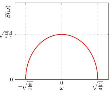
Figure 2: The spectral function eq. (38) of the semi-infinite chain assumes a semi-elliptic shape.

V Inverse Laplace transform

In order to compute the inverse Laplace transform one can either compute the Bromwich integral or make use of correspondence tablesAbramowitzStegun . A correspondence to (36) can directly be found in such a table:

$$\mathcal{L}\left\{{q_{0}}\right\}=Q_{0}=\mathcal{L}\left\{{\frac{2A}{\sqrt{\frac{4k}{m}}t}J_{1}\left(\sqrt{\frac{4k}{m}}t\right)}\right\}\ ,$$ (39)

where $J_{1}$ is the Bessel function of the first kind. We conclude that the time dependence of the displacement of the zeroth mass point is given by

$$q_{0}(t)=\frac{2A}{\sqrt{\frac{4k}{m}}t}J_{1}\left(\sqrt{\frac{4k}{m}}t\right).$$ (40)

As shown in Fig. 3, the displacement $q_{0}(t)$ describes the expected damped oscillation of the first oscillator due to the coupling to the chain.

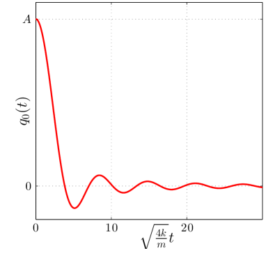
Figure 3: Sketch of the solution $q_{0}(t)$, eq. (40), for an initial value of $q_{0}(0)=A$.

In what follows the recurrence relations for the Bessel functionsAbramowitzStegun are required

$$\frac{2n}{\bar{\omega}t}J_{n}\left(\bar{\omega}t\right)=J_{n-1}\left(\bar{\omega}t\right)+J_{n+1}\left(\bar{\omega}t\right)\ ,$$ (41)

$$\frac{2}{\bar{\omega}}\frac{\partial}{\partial t}J_{n}\left(\bar{\omega}t\right)=J_{n-1}\left(\bar{\omega}t\right)-J_{n+1}\left(\bar{\omega}t\right)\ .$$ (42)

With the help of (41) we can write

$$q_{0}(t)=AJ_{2}\left(\sqrt{\frac{4k}{m}}t\right)+AJ_{0}\left(\sqrt{\frac{4k}{m}}t\right).$$ (43)

We then find by solving (20) for $q_{1}$ and using (42) that

$$q_{1}(t) =AJ_{4}\left(\sqrt{\frac{4k}{m}}t\right)+AJ_{2}\left(\sqrt{\frac{4k}{m}}t\right)$$ (44)

$$=\frac{6A}{\sqrt{\frac{4k}{m}}t}J_{3}\left(\sqrt{\frac{4k}{m}}t\right).$$ (45)

Using (21) as a recursion relation we find for the remaining displacements by induction that

$$q_{n}(t)=\frac{(4n+2)A}{\sqrt{\frac{4k}{m}}t}J_{2n+1}\left(\sqrt{\frac{4k}{m}}t\right).$$ (46)

In an analogous calculation one finds for the initial conditions

$$q_{n}(0)=0,\quad p_{n}(0)=P\cdot\delta_{n,0}\quad\text{for }n=0,1,2,\ldots$$ (47)

that

$$Q_{0}(s)=\frac{1}{s}\frac{2P/m}{s+\sqrt{s^{2}+\frac{4k}{m}}}.$$ (48)

Under employment of eq. (10) one then finds

$$q_{n}(t)=\frac{(4n+2)P}{m}\int\limits_{0}^{t}\textnormal{d}\tau\frac{J_{2n+1}\left(\sqrt{\frac{4k}{m}}\tau\right)}{\sqrt{\frac{4k}{m}}\tau}.$$ (49)

In the calculation of (49) certain steps where skipped as they are similar to the ones appearing in the calculation of (43). The final value theorem tells us then that $\lim\limits_{t\rightarrow\infty}q_{0}(t)=P/\sqrt{km}$. The initial condition (47) thus leads to a shift of the equilibrium positions by a factor $P/\sqrt{km}$. The solutions (43) and (49) coincide with the solutions one obtains by Goodman’s methodGoodman , the normal mode expansion.

VI generalizations

In this section, we briefly discuss an infinite chain as sketched in Fig. 4. The Hamiltonian for this system is given by

$$H=\sum_{n=-\infty}^{\infty}\frac{p_{n}^{2}}{2m}+\sum_{n=-\infty}^{\infty}\frac{k}{2}(q_{n+1}-q_{n})^{2}\ .$$ (50)

We choose the initial conditions

$$q_{n}(0)=A\delta_{n,0},\quad p_{n}(0)=0\quad\text{for all }n\in\mathbb{Z}.$$ (51)

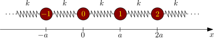
Figure 4: Sketch of the infinite harmonic chain, corresponding to the Hamiltonian eq. (50).

For simplicity, we take equal masses $m_{n}=m$ and equal spring constants $k_{n}=k$. The symmetry of the system now implies

$$q_{n}(t)=q_{-n}(t)\quad\text{ for all }t\geq 0.$$ (52)

To show this explicitly, we define a new set of canonical coordinates by

$$q^{\pm}_{n} :=\frac{1}{2}(q_{n}\pm q_{-n}) \text{for }n>0$$ (53)

$$p^{\pm}_{n} :=p_{n}\pm p_{-n} \text{for }n>0$$ (54)

In the new coordinates, $H$ has the form

$$H =\frac{p_{0}^{2}}{2m}+\frac{1}{4m}\sum_{n=1}^{\infty}\left(p_{n}^{+}\right)^{2}$$

$$+\frac{2k}{2}\left[\left(q_{0}-q_{1}^{+}\right)^{2}+\sum_{n=1}^{\infty}\left(q_{n+1}^{+}-q_{n}^{+}\right)^{2}\right]$$

$$+\frac{1}{4m}\sum_{n=1}^{\infty}\left(p_{n}^{-}\right)^{2}+\frac{2k}{2}\left[\left(q_{1}^{-}\right)^{2}+\sum_{n=1}^{\infty}\left(q_{n+1}^{-}-q_{n}^{-}\right)^{2}\right]$$ (55)

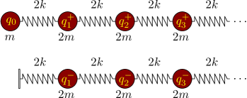
Figure 5: Sketch of the harmonic chain, after the canonical transformation described in the text. The infinite chain can be mapped onto a semi-infinite chain with modified parameters, and a decoupled chain.

$H$ now has the form of a Hamiltonian that describes a system of two decoupled chains as sketched in Fig. 5. The coordinate $q_{0}$ couples to a semi-infinite chain whose mass points have coordinates $q_{n}^{+}$. In addition, there is a second semi-infinite chain of mass points with coordinates $q_{n}^{-}$ that is decoupled from $q_{0}$ and obeys fixed boundary conditions as shown in Fig. 5. It follows that if we choose initial conditions such that $q_{n}^{-}(0)=0$ for all $n>0$ then $q_{n}^{-}(t)=\frac{1}{2}[q_{n}(t)-q_{-n}(t)]=0$ for all $t\geq 0$. Thus we conclude that the initial conditions (51) fulfill $q_{n}(t)=q_{-n}(t)$ at all times.

Moreover, we can simply use the continued fraction eq. (29) and plug in the spring constants and masses accordingly, i.e.

$$k_{0}=2k,\ k_{1}=2k,\ k_{2}=2k,\ \dots$$

$$m_{0}=m,\ m_{1}=2m,\ m_{2}=2m,\ \dots$$ (56)

to obtain the continued fraction expression for the Laplace transform of the displacement of the zeroth mass point which then takes the form

$$Q_{0}(s)=\cfrac{As}{\frac{2k}{m}+s^{2}-\frac{2k^{2}}{m^{2}}\cfrac{1}{\frac{2k}{m}+s^{2}-\frac{k^{2}}{m^{2}}\cfrac{1}{\frac{2k}{m}+s^{2}-\frac{k^{2}}{m^{2}}\cfrac{1}{\ddots}}}}\ .$$ (57)

By recognizing the periodicity of the continued fraction, the expression for $Q_{0}(s)$ can be simplified to

$$Q_{0}(s)=\pm\frac{A}{\sqrt{\frac{4k}{m}+s^{2}}}.$$ (58)

The ambiguity in the sign can again be dissolved by using the initial value theorem, which then provides us with the unique solution

$$Q_{0}(s)=\frac{A}{\sqrt{\frac{4k}{m}+s^{2}}}.$$ (59)

The spectral function for this case reads (see Fig. 6):

$$S(\omega)=\frac{A}{\pi}\begin{cases}\frac{1}{\sqrt{\frac{4k}{m}-\omega^{2}}}&\mbox{if }|\omega|\leq\sqrt{\frac{4k}{m}}\ ,\\ \quad 0&\mbox{if }|\omega|>\sqrt{\frac{4k}{m}}\ .\end{cases}$$ (60)

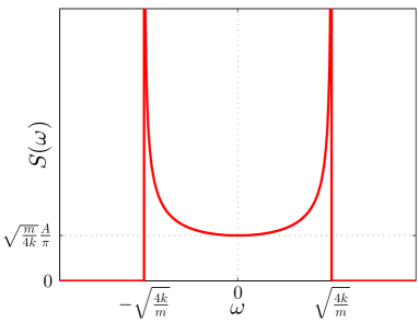
Figure 6: The spectral function of the infinite chain, eq. (60)

Comparison of eq. (59) with the Laplace transform of the zeroth Bessel function yields

$$q_{0}(t)=AJ_{0}\left(\sqrt{\frac{4k}{m}}t\right).$$ (61)

The Newtonian equations of motion are given by

$$\ddot{q}_{n}=\frac{k}{m}\left(q_{n-1}+q_{n+1}\right)-\frac{2k}{m}q_{n}.$$ (62)

For the case $n=0$ we find by using eq. (52) that

$$\frac{2k}{m}q_{1}=\ddot{q}_{0}+\frac{2k}{m}q_{0}.$$ (63)

Which gives us by employing the recurrence relations (41,42) of the Bessel functions that

$$q_{1}(t)=AJ_{2}\left(\sqrt{\frac{4k}{m}}t\right).$$ (64)

Rearranging eq. (62) gives the recursion relation

$$q_{n+1}=\left(\frac{m}{k}\frac{d^{2}}{dt^{2}}+2\right)q_{n}-q_{n-1}.$$ (65)

Using this and the recurrance relations (41,42) we find by induction that

$$q_{n}(t)=AJ_{2n}\left(\sqrt{\frac{4k}{m}}t\right).$$ (66)

Figure 7a shows the positions $x_{n}(t)=q_{n}(t)+na$ for $n=0,1,\ldots,4$. One can clearly see how the initial displacement of site $0$ spreads through the chain, with the first maximum for each $x_{n}(t)$ moving with the speed of sound of the harmonic chain, while the individual displacements are damped due to the coupling to the rest of the chain. Note that this damping (for $n=0$) is significantly reduced as compared to the semi-infinite case, Fig. (3).

In an analogous calculation one finds for the initial values

$$q_{n}(0)=0,\quad p_{n}(0)=P\cdot\delta_{n,0}\quad\text{for all }n\in\mathbb{Z}\ ,$$ (67)

that the Laplace transform of the zeroth displacement is given by

$$Q_{0}(s)=\frac{P/m}{s\sqrt{\frac{4k}{m}+s^{2}}}$$ (68)

from which one finds $\lim\limits_{t\rightarrow\infty}q_{0}(t)=P/\sqrt{4km}$. The displacements are given by

$$q_{n}(t)=\frac{P}{m}\int_{0}^{t}\textnormal{d}\tau J_{2n}\left(\sqrt{\frac{4k}{m}}\tau\right).$$ (69)

The solutions (66) and (69) again match with those obtained by a normal mode expansionGoodman . Just like in the previous section the choice of non-vanishing initial momenta leads to a shift of equilibrium positions (see Fig. 7b), this time by a factor $P/\sqrt{4km}$ which is half the factor one obtains in the case of the semi infinite chain.

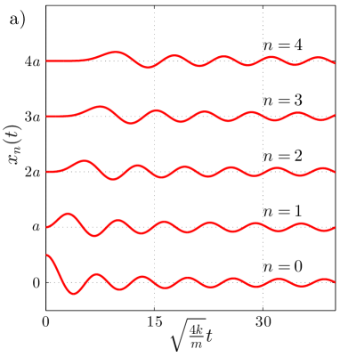
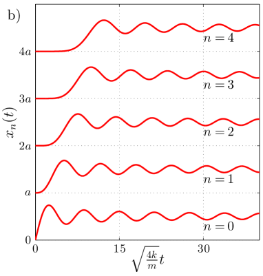
Figure 7: Plot of the positions $x_{n}(t)=q_{n}(t)+na$ as given in eqs. (66) and (69) for the initial conditions: (a) $q_{0}(0)=A$ and $p_{0}(0)=0$, (b) $q_{0}(0)=0$ and $p_{0}(0)=P$.

VII Comparison to the quantum case

Let us now turn to a quantum many-particle system which, at first sight, has not much in common with the classical harmonic chain discussed so far. The Hamiltonian of a one-dimensional tight-binding chain of spinless fermions takes the form

$$H=\sum_{n=0}^{N}\varepsilon_{n}c_{n}^{\dagger}c_{n}+\sum_{n=0}^{N-1}t_{n}\left(c_{n}^{\dagger}c_{n+1}+c_{n+1}^{\dagger}c_{n}\right)\ ,$$ (70)

with $c_{n}^{(\dagger)}$ fermionic creation (annihilation) operators and the parameters $\varepsilon_{n}$ and $t_{n}$ corresponding to onsite energies and hopping matrix elements, respectively.

Of particular interest in the theoretical investigation of quantum many-particle systems are Green functions of the form Mahan

$$G_{ij}(z)\equiv\langle\!\langle c_{i},c_{j}^{\dagger}\rangle\!\rangle_{z}=\int_{0}^{\infty}{\rm d}t\,e^{izt}X_{ij}(t)\ ,$$ (71)

with

$$X_{ij}(t)=-i\theta(t)\langle[c_{i}(t),c_{j}^{\dagger}]_{+}\rangle\ .$$ (72)

The Green function $\langle\!\langle c_{i},c_{j}^{\dagger}\rangle\!\rangle_{z}$ is given by the Laplace transform of the time-dependent correlation function $X_{ij}(t)$ – note that we use here the usual convention of quantum many-particle theory (with $z=\omega+i\delta$, $\delta>0$) different to the Laplace transform as introduced in Sec. II. The Green function is now an analytic function in the whole upper complex plane. This convention for the Laplace transform is related to the previous definition given in eq. (2) via

$$\int_{0}^{\infty}{\rm d}t\ e^{izt}f(t)=-i\mathcal{L}\left\{{f}\right\}\left({s=-iz}\right)\ .$$ (73)

The equation of motion for the Green function $\langle\!\langle A,B\rangle\!\rangle_{z}$ takes the form

$$z\langle\!\langle A,B\rangle\!\rangle_{z}+\langle\!\langle LA,B\rangle\!\rangle_{z}=\langle[A,B]_{+}\rangle\ ,$$ (74)

(with $LA:=[H,A]_{-}$) in close analogy to eq. (17). In contrast to the classical case, there is no need for a second order equation of motion here, simply because the Schrödinger equation is a first order differential equation in time.

Application of the equation of motion to the Green functions $G_{n}(z):=\langle\!\langle c_{n},c_{0}^{\dagger}\rangle\!\rangle_{z}$ generates a set of equations which can be brought into the form of a continued fraction, with the final result given by

$$G_{0}(z)=\cfrac{1}{z-\varepsilon_{0}-\cfrac{t_{0}^{2}}{z-\varepsilon_{1}-\cfrac{t_{1}^{2}}{z-\varepsilon_{2}-\ldots}}}\ .$$ (75)

For equal $\varepsilon_{n}=\varepsilon$, $t_{n}=t$ and in the limit $N\to\infty$, the continued fraction results in the expression

$$G_{0}(z)=\frac{1}{2t^{2}}\left(z-\varepsilon-\sqrt{(z-\varepsilon)^{2}-4t^{2}}\right)\ .$$ (76)

The corresponding spectral function is now defined via the imaginary part of the Green function:

$$A(\omega)=-\frac{1}{\pi}\lim_{\delta\to 0}{\rm Im}G(z=\omega+i\delta)\ ,$$ (77)

which results in

$$A(\omega)=\frac{1}{2\pi t^{2}}\begin{cases}\sqrt{4t^{2}-(\omega-\varepsilon)^{2}}&\mbox{if }|\omega-\varepsilon|\leq 2t\\ \quad 0&\mbox{if }|\omega-\varepsilon|>2t\end{cases}$$ (78)

again giving the semi-elliptic shape as in Fig. 2.

Although we omitted a couple of steps here (such as the calculation of the commutators $LA$), the analogy to the procedure given in Sec. IV is obvious.

VIII summary

In this paper we presented a method to calculate analytically the displacements $q_{n}(t)$ of a classical harmonic chain, with the focus on semi-infinite and infinite geometries for which various initial conditions were studied. The calculation proceeds via equations of motion for the Laplace transforms $Q_{n}(s):=\mathcal{L}\left\{{q_{n}}\right\}\left({s}\right)$ and results in a continued fraction expression for $Q_{0}(s)$. Finally, the displacements $q_{n}(t)$ are obtained through an inverse Laplace transformation of the $Q_{n}(s)$, with the $q_{n}(t)$ acquiring the form of Bessel functions.

We believe that the models and the calculations as presented in this paper would be useful as part of a lecture on classical (analytical) mechanics. While some of the derivations shown here can certainly be used as exercises in problem classes, students might also profit from studying the harmonic chain numerically, i.e. solving the set of coupled differential equations for the $q_{n}(t)$. The numerical results for either $q_{n}(t)$ or $Q_{0}(s)$ (from a subsequent numerical Laplace transformation) can then be compared with the analytical expressions.

The concept of using equations of motion for the Laplace transforms $\mathcal{L}\left\{{q_{n}}\right\}\left({s}\right)$ might also serve as a useful preparation for a course on quantum many-particle systems. As discussed briefly in Sec. VII, there are close analogies between the approach presented here for a classical harmonic chain and the Green function approach for a quantum-mechanical tight-binding chain.

IX acknowledgments

We would like to thank Matthias Herzkamp for pointing out that the continued fraction eq. (30) can be most efficiently derived by rearranging the equations of motion as in eqs. (25) and (28). Part of this work was funded through the Institutional Strategy of the University of Cologne within the German Excellence Initiative.

References

- (1) M. Abramowitz, I. Stegun (1965) Handbook of Mathematical Functions, Dover Publications.
- (2) J. Honerkamp, H. Römer (1993) Theoretical Physics: A Classical Approach, Springer Verlag.
- (3) R. Douglas Gregory (2006) Classical Mechanics, Cambridge.
- (4) F. Kuypers (2010) Klassische Mechanik, Wiley-VCH.
- (5) F.O. Goodman, “Propagation of a Disturbance on a One-Dimensional Lattice Solved by Response Functions”, Am. J. Phys. 40, 92 (1972).
- (6) S.A. Cannas and D. Prato, “Externally excited semi‐infinite one‐dimensional models”, Am. J. Phys. 59, 915 (1991)
- (7) D.L. Merchant and O.L. Brill, “Propagation of a Localized Impulse on a One-Dimensional Lattice”, Am. J. Phys. 41, 55 (1973).
- (8) G.D. Mahan (1981) Many-Particle Physics, Plenum Press.