Abstract

We derive Fredholm determinant representation for isomonodromic tau functions of Fuchsian systems with $n$ regular singular points on the Riemann sphere and generic monodromy in $\mathrm{GL}\left(N,\mathbb{C}\right)$. The corresponding operator acts in the direct sum of $N\left(n-3\right)$ copies of $L^{2}\left(S^{1}\right)$. Its kernel has a block integrable form and is expressed in terms of fundamental solutions of $n-2$ elementary 3-point Fuchsian systems whose monodromy is determined by monodromy of the relevant $n$-point system via a decomposition of the punctured sphere into pairs of pants. For $N=2$ these building blocks have hypergeometric representations, the kernel becomes completely explicit and has Cauchy type. In this case Fredholm determinant expansion yields multivariate series representation for the tau function of the Garnier system, obtained earlier via its identification with Fourier transform of Liouville conformal block (or a dual Nekrasov-Okounkov partition function). Further specialization to $n=4$ gives a series representation of the general solution to Painlev VI equation.

1 Introduction

1.1 Motivation and some results

The theory of monodromy preserving deformations plays a prominent role in many areas of modern nonlinear mathematical physics. The classical works [WMTB, JMMS, TW1] relate, for instance, various correlation and distribution functions of statistical mechanics and random matrix theory models to special solutions of Painlevé equations. The relevant Painlev functions are usually written in terms of Fredholm or Toeplitz determinants. Further study of these relations has culminated in the development by Tracy and Widom [TW2] of an algorithmic procedure of derivation of systems of PDEs satisfied by Fredholm determinants with integrable kernels [IIKS] restricted to a union of intervals; the isomonodromic origin of Tracy-Widom equations has been elucidated in [Pal2] and further studied in [HI]. This raises a natural question:

• Can the general solution of isomonodromy equations be expressed in terms of a Fredholm determinant?

One of the goals of the present paper is to provide a constructive answer to this question in the Fuchsian setting. Let us consider a Fuchsian system with $n$ regular singular points $a:=\left\{a_{0},\ldots,a_{n-2},a_{n-1}\equiv\infty\right\}$ on ${\mathbb{P}^{1}\equiv\mathbb{P}^{1}\left(\mathbb{C}\right)}$:

$$\partial_{z}\Phi=\Phi A\left(z\right),\qquad A\left(z\right)=\sum_{k=0}^{n-2}\frac{A_{k}}{z-a_{k}},$$ (1.1)

where $A_{0},\ldots,A_{n-2}$ are $N\times N$ matrices independent of $z$ and $\Phi\left(z\right)$ is a fundamental matrix solution, multivalued on $\mathbb{P}^{1}\backslash a$. The monodromy of $\Phi\left(z\right)$ realizes a representation of the fundamental group $\pi_{1}\left(\mathbb{P}^{1}\backslash a\right)$ in $\mathrm{GL}\left(N,\mathbb{C}\right)$. When the residue matrices $A_{0},\ldots,A_{n-2}$ and $A_{n-1}:=-\sum_{k=0}^{n-2}A_{k}$ are non-resonant, the isomonodromy equations are given by the Schlesinger system,

$$\begin{cases}\partial_{a_{i}}A_{k}=&\displaystyle\frac{\left[A_{i},A_{k}\right]}{a_{k}-a_{i}},\qquad\qquad i\neq k,\\ \partial_{a_{i}}A_{i}=&\displaystyle\sum_{k\neq i}\frac{\left[A_{i},A_{k}\right]}{a_{i}-a_{k}}.\end{cases}$$ (1.2)

Integrating the flows associated to affine transformations, we may set without loss of generality $a_{0}=0$ and $a_{n-2}=1$, so that there remains $n-3$ nontrivial time variables $a_{1},\ldots,a_{n-3}$. In the case ${N=2}$, Schlesinger equations reduce to the Garnier system $\mathcal{G}_{n-3}$, see for example [IKSY, Chapter 3] for the details. Setting further $n=4$, we are left with only one time $t\equiv a_{1}$ and the latter system becomes equivalent to a nonlinear 2nd order ODE — the Painlev  VI equation.

The main object of our interest is the isomonodromic tau function of Jimbo-Miwa-Ueno [JMU]. It is defined as an exponentiated primitive of the $1$-form

$$d_{a}\ln\tau_{\mathrm{JMU}}:=\frac{1}{2}\sum_{k=0}^{n-2}\operatorname{res}_{z=a_{k}}\operatorname{Tr}A^{2}\left(z\right)\;da_{k}.$$ (1.3)

The definition is consistent since the 1-form on the right is closed on solutions of the deformation equations (1.2). It generates the hamiltonians of the Schlesinger system. Dealing with the Garnier system, we will assume the standard gauge where $\operatorname{Tr}A\left(z\right)=0$ and denote the eigenvalues of $A_{k}$ by $\pm\theta_{k}$ with $k=0,\ldots,n-1$. In the Painlev  VI case, it is convenient to modify this notation as $\left(\theta_{0},\theta_{1},\theta_{2},\theta_{3}\right)\mapsto\left(\theta_{0},\theta_{t},\theta_{1},\theta_{\infty}\right)$. The logarithmic derivative $\zeta\left(t\right):=t\left(t-1\right)\frac{d}{dt}\ln\tau_{\mathrm{VI}}\left(t\right)$ then satisfies the $\sigma$-form of Painlev VI,

$$\Bigl{(}t(t-1)\zeta^{\prime\prime}\Bigr{)}^{2}=-2\;\mathrm{det}\left(\begin{array}[]{ccc}2\theta_{0}^{2}&t\zeta^{\prime}-\zeta&\zeta^{\prime}+\theta_{0}^{2}+\theta_{t}^{2}+\theta_{1}^{2}-\theta_{\infty}^{2}\\ t\zeta^{\prime}-\zeta&2\theta_{t}^{2}&(t-1)\zeta^{\prime}-\zeta\\ \zeta^{\prime}+\theta_{0}^{2}+\theta_{t}^{2}+\theta_{1}^{2}-\theta_{\infty}^{2}&(t-1)\zeta^{\prime}-\zeta&2\theta_{1}^{2}\end{array}\right).$$ (1.4)

Monodromy of the associated linear problems provides a complete set of conserved quantities for Painlev  VI, the Garnier system and Schlesinger equations. By the general solution of deformation equations we mean the solution corresponding to generic monodromy data. The precise genericity conditions will be specified in the main body of the text.

In [Pal1], Palmer (developing earlier results of Malgrange [Mal] and Sato-Segal-Wilson [Sato, SW]) interpreted the Jimbo-Miwa-Ueno tau function (1.3) as a determinant of a singular Cauchy-Riemann operator acting on functions with prescribed monodromy. The main idea of [Pal1] is to isolate the singular points $a_{0},\ldots,a_{n-1}$ inside a circle $\mathcal{C}\subset\mathbb{P}^{1}$ and represent the Fuchsian system (1.1) by a boundary space of functions on $\mathcal{C}$ that can be analytically continued inside with specified branching. The variation of positions of singularities gives rise to a trajectory of this space in an infinite Grassmannian. The tau function is obtained by comparing two sections of an associated determinant bundle.

The construction suggested in the present paper is essentially a refinement of Palmer’s approach, translated into the Riemann-Hilbert framework. A single circle $\mathcal{C}$ is replaced by the boundaries of $n-3$ annuli which cut the $n$-punctured sphere $\mathbb{P}^{1}\backslash a$ into trinions (pairs of pants), see e.g. Fig. 2a below. To each trinion is assigned a Fuchsian system with 3 regular singular points whose monodromy is determined by monodromy of the original system. We show that the isomonodromic tau function is proportional to a Fredholm determinant:

$$\tau_{\mathrm{JMU}}\left(a\right)=\Upsilon\left(a\right)\cdot\operatorname{det}\left(\mathbb{1}-K\right),$$ (1.5)

where the prefactor $\Upsilon\left(a\right)$ is a known elementary function. The integral operator $K$ acts on holomorphic vector functions on the union of annuli and involves projections on certain boundary spaces.

The pay-off of a more complicated Grassmannian model is that the kernel of $K$ may be written explicitly in terms of $3$-point solutions. In particular, for $N=2$ (i.e. for the Garnier system) the latter have hypergeometric expressions. The $n=4$ specialization of our result is as follows.

Theorem A.

Let the independent variable $t$ of Painlev VI equation vary inside the real interval $]0,1[$ and let $\mathcal{C}=\left\{z\in\mathbb{C}\,:\,|z|=R,t<R<1\right\}$ be a counter-clockwise oriented circle. Let $\sigma$, $\eta$ be a pair of complex parameters satisfying the conditions

$$\left|\Re\sigma\right|\leq\frac{1}{2},\qquad\sigma\neq 0,\pm\frac{1}{2},$$

$$\theta_{0}\pm\theta_{t}+\sigma\notin\mathbb{Z},\qquad\theta_{0}\pm\theta_{t}-\sigma\notin\mathbb{Z},\qquad\theta_{1}\pm\theta_{\infty}+\sigma\notin\mathbb{Z},\qquad\theta_{1}\pm\theta_{\infty}-\sigma\notin\mathbb{Z}.$$

General solution of the Painlev VI equation (1.4) admits the following Fredholm determinant representation:

$$\tau_{\mathrm{VI}}\left(t\right)=\mathrm{const}\cdot t^{\sigma^{2}-\theta_{0}^{2}-\theta_{t}^{2}}\left(1-t\right)^{-2\theta_{t}\theta_{1}}\operatorname{det}\left(\mathbb{1}-U\right),\qquad U=\left(\begin{array}[]{cc}0&\mathsf{a}\\ \mathsf{d}&0\end{array}\right),$$ (1.6)

where the operators $\mathsf{a},\mathsf{d}\in\operatorname{End}\left(\mathbb{C}^{2}\otimes L^{2}\left(\mathcal{C}\right)\right)$ act on $g=\left(\begin{array}[]{c}g_{+}\\ g_{-}\end{array}\right)$ with $g_{\pm}\in L^{2}\left(\mathcal{C}\right)$ as

$$\left(\mathsf{a}g\right)\left(z\right)=\,\frac{1}{2\pi i}\oint_{\mathcal{C}}\,\mathsf{a}\left(z,z^{\prime}\right)g\left(z^{\prime}\right)dz^{\prime}\,,\qquad\left(\mathsf{d}g\right)\left(z\right)=\,\frac{1}{2\pi i}\oint_{\mathcal{C}}\mathsf{d}\left(z,z^{\prime}\right)g\left(z^{\prime}\right)dz^{\prime},$$ (1.7)

and their kernels are explicitly given by

$$\mathsf{a}\left(z,z^{\prime}\right)= \,\frac{\left(1-z^{\prime}\right)^{2\theta_{1}}\left(\begin{array}[]{cc}K_{++}\left(z\right)&K_{+-}\left(z\right)\\ K_{-+}\left(z\right)&K_{--}\left(z\right)\end{array}\right)\left(\begin{array}[]{rr}K_{--}\left(z^{\prime}\right)&\!\!\!-K_{+-}\left(z^{\prime}\right)\\ \!\!\!-K_{-+}\left(z^{\prime}\right)&K_{++}\left(z^{\prime}\right)\end{array}\right)-\mathbb{1}}{z-z^{\prime}},$$ (1.8)

$$\mathsf{d}\left(z,z^{\prime}\right)= \,\frac{\mathbb{1}-\left(1-\frac{t}{z^{\prime}}\right)^{2\theta_{t}}\left(\begin{array}[]{cc}\bar{K}_{++}\left(z\right)&\bar{K}_{+-}\left(z\right)\\ \bar{K}_{-+}\left(z\right)&\bar{K}_{--}\left(z\right)\end{array}\right)\left(\begin{array}[]{cc}\bar{K}_{--}\left(z^{\prime}\right)&-\bar{K}_{+-}\left(z^{\prime}\right)\\ -\bar{K}_{-+}\left(z^{\prime}\right)&\bar{K}_{++}\left(z^{\prime}\right)\end{array}\right)}{z-z^{\prime}},$$

with

$$K_{\pm\pm}\left(z\right)= \,{}_{2}F_{1}\biggl{[}\begin{array}[]{c}\theta_{1}+\theta_{\infty}\pm\sigma,\theta_{1}-\theta_{\infty}\pm\sigma\\ \pm 2\sigma\end{array};z\biggr{]},$$ (1.9)

$$K_{\pm\mp}\left(z\right)= \,\pm\frac{\theta_{\infty}^{2}-\left(\theta_{1}\pm\sigma\right)^{2}}{2\sigma\left(1\pm 2\sigma\right)}\,z\,{}_{2}F_{1}\biggl{[}\begin{array}[]{c}1+\theta_{1}+\theta_{\infty}\pm\sigma,1+\theta_{1}-\theta_{\infty}\pm\sigma\\ 2\pm 2\sigma\end{array};z\biggr{]},$$

$$\bar{K}_{\pm\pm}\left(z\right)= \,{}_{2}F_{1}\biggl{[}\begin{array}[]{c}\theta_{t}+\theta_{0}\mp\sigma,\theta_{t}-\theta_{0}\mp\sigma\\ \mp 2\sigma\end{array};\frac{t}{z}\biggr{]},$$

$$\bar{K}_{\pm\mp}\left(z\right)= \,\mp t^{\mp 2\sigma}e^{\mp i\eta}\frac{\theta_{0}^{2}-\left(\theta_{t}\mp\sigma\right)^{2}}{2\sigma\left(1\mp 2\sigma\right)}\,\frac{t}{z}\,{}_{2}F_{1}\biggl{[}\begin{array}[]{c}1+\theta_{t}+\theta_{0}\mp\sigma,1+\theta_{t}-\theta_{0}\mp\sigma\\ 2\mp 2\sigma\end{array};\frac{t}{z}\biggr{]}.$$

Moreover, we demonstrate that for a special choice of monodromy in the Painlev VI case, $U$ becomes equivalent to the hypergeometric kernel of [BO1] and thereby reproduces previously known family of Fredholm determinant solutions [BD]. The hypergeometric kernel is known to produce other random matrix integrable kernels in confluent limits.

Another part of our motivation comes from isomonodromy/CFT/gauge theory correspondence. It was conjectured in [GIL12] that the tau function associated to the general Painlev VI solution coincides with a Fourier transform of $4$-point $c=1$ Virasoro conformal block with respect to its intermediate momentum. Two independent derivations of this conjecture have been already proposed in [ILTe] and [BSh]. The first approach [ILTe] also extends the initial statement to the Garnier system. Its main idea is to consider the operator-valued monodromy of conformal blocks with additional level 2 degenerate insertions. At $c=1$, Fourier transform of such conformal blocks reduces their “quantum” monodromy to ordinary $2\times 2$ matrices. It can therefore be used to construct the fundamental matrix solution of a Fuchsian system with prescribed $\mathrm{SL}\left(2,\mathbb{C}\right)$ monodromy. The second approach [BSh] uses an embedding of two copies of the Virasoro algebra into super-Virasoro algebra extended by Majorana fermions to prove certain bilinear differential-difference relations for $4$-point conformal blocks, equivalent to Painlev  VI equation. An interesting feature of this method is that bilinear relations admit a deformation to generic values of Virasoro central charge.

Among other developments, let us mention the papers [GIL13, ILT14, Nag] where asymptotic expansions of Painlev V, IV and III tau functions were identified with Fourier transforms of irregular conformal blocks of different types. The study of relations between isomonodromy problems in higher rank and conformal blocks of $W_{N}$ algebras has been initiated in [Gav, GM1, GM2].

The AGT conjecture [AGT] (proved in [AFLT]) identifies Virasoro conformal blocks with partition functions of $\mathcal{N}=2$ 4D supersymmetric gauge theories. There exist combinatorial representations of the latter objects [Nek], expressing them as sums over tuples of Young diagrams. This fact is of crucial importance for isomonodromy theory, since it gives (contradicting to an established folklore) explicit series representations for the Painlev  VI and Garnier tau functions. Since the very first paper [GIL12] on the subject, there has been a puzzle to understand combinatorial tau function expansions directly within the isomonodromic framework. There have also been attempts to sum up these series to determinant expressions; for example, in [Bal] truncated infinite series for $c=1$ conformal blocks were shown to coincide with partition functions of certain discrete matrix models.

In this work, we show that combinatorial series correspond to the principal minor expansion of the Fredholm determinant (1.5), written in the Fourier basis of the space of functions on annuli of the pants decomposition. Fourier modes which label the choice of rows for the principal minor are related to Frobenius coordinates of Young diagrams. It should be emphasized that this combinatorial structure is valid also for $N>2$ where CFT/gauge theory counterparts of the tau functions have yet to be defined and understood.

We prove in particular the following result, originally conjectured in [GIL12] (the details of notation concerning Young diagrams are explained in the next subsection):

Theorem B.

General solution of the Painlev VI equation (1.4) can be written as

$$\tau_{\mathrm{VI}}(t)=\operatorname{const}\cdot\sum_{n\in\mathbb{Z}}e^{in\eta^{\prime}}\mathcal{B}\left(\vec{\theta};\sigma+n;t\right),$$ (1.10)

where $\mathcal{B}(\vec{\theta},\sigma;t)$ is a double sum over Young diagrams,

$$\mathcal{B}\left(\vec{\theta},\sigma;t\right)=\mathcal{N}_{\theta_{\infty},\sigma}^{\theta_{1}}\mathcal{N}_{\sigma,\theta_{0}}^{\theta_{t}}t^{\sigma^{2}-\theta_{0}^{2}-\theta_{t}^{2}}(1-t)^{2\theta_{t}\theta_{1}}\sum_{\lambda,\mu\in\mathbb{Y}}\mathcal{B}_{\lambda,\mu}\left(\vec{\theta},\sigma\right)t^{|\lambda|+|\mu|},$$

$$\mathcal{B}_{\lambda,\mu}\left(\vec{\theta},\sigma\right)=\!\!\!\!\prod_{(i,j)\in\lambda}\!\!\!\!\frac{\left(\left(\theta_{t}+\sigma+i-j\right)^{2}-\theta_{0}^{2}\right)\left(\left(\theta_{1}+\sigma+i-j\right)^{2}-\theta_{\infty}^{2}\right)}{h_{\lambda}^{2}(i,j)\left(\lambda^{\prime}_{j}-i+\mu_{i}-j+1+2\sigma\right)^{2}}\!\!\!\!\prod_{(i,j)\in\mu}\!\!\!\!\frac{\left(\left(\theta_{t}-\sigma+i-j\right)^{2}-\theta_{0}^{2}\right)\left(\left(\theta_{1}-\sigma+i-j\right)^{2}-\theta_{\infty}^{2}\right)}{h_{\mu}^{2}(i,j)\left(\mu^{\prime}_{j}-i+\lambda_{i}-j+1-2\sigma\right)^{2}}\,,$$

$$\mathcal{N}_{\theta_{3},\theta_{1}}^{\theta_{2}}=\frac{\prod_{\epsilon=\pm}G\left(1+\theta_{3}+\epsilon(\theta_{1}+\theta_{2})\right)G\left(1-\theta_{3}+\epsilon(\theta_{1}-\theta_{2})\right)}{G(1-2\theta_{1})G(1-2\theta_{2})G(1+2\theta_{3})}.$$

Here $\sigma\notin\mathbb{Z}/2$, $\eta^{\prime}$ are two arbitrary complex parameters, and $G\left(z\right)$ denotes the Barnes $G$-function.

The parameters $\sigma$ play exactly the same role in the Fredholm determinant (1.6) and the series representation (1.10), whereas $\eta$ and $\eta^{\prime}$ are related by a simple transformation. An obvious quasiperiodicity of the second representation with respect to integer shifts of $\sigma$ is by no means manifest in the Fredholm determinant.

1.2 Notation

The monodromy matrices of Fuchsian systems and the jumps of associated Riemann-Hilbert problems appear on the left of solutions. These somewhat unusual conventions are adopted to avoid even more confusing right action of integral and infinite matrix operators. The indices corresponding to the matrix structure of rank $N$ Riemann-Hilbert problem are referred to as color indices and are denoted by Greek letters, such as $\alpha,\beta\in\left\{1,\ldots,N\right\}$. Upper indices in square brackets, e.g. $[k]$ in $\mathcal{T}^{[k]}$, label different trinions in the pants decomposition of a punctured Riemann sphere. We denote by $\mathbb{Z}^{\prime}:=\mathbb{Z}+\frac{1}{2}$ the half-integer lattice, and by $\mathbb{Z}^{\prime}_{\pm}=\left\{p\in\mathbb{Z}^{\prime}\,|\,p\gtrless 0\right\}$ its positive and negative parts. The elements of $\mathbb{Z}^{\prime},\mathbb{Z}^{\prime}_{\pm}$ will be generally denoted by the letters $p$ and $q$.

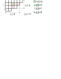
Figure 1: Young diagram associated to the partition $\lambda=\left\{6,5,4,2\right\}$.

The set of all partitions identified with Young diagrams is denoted by $\mathbb{Y}$. For $\lambda\in\mathbb{Y}$, we write $\lambda^{\prime}$ for the transposed diagram, $\lambda_{i}$ and $\lambda^{\prime}_{j}$ for the number of boxes in the $i$th row and $j$th column of $\lambda$, and $|\lambda|$ for the total number of boxes in $\lambda$. Let $\square=\left(i,j\right)$ be the box in the $i$th row and $j$th column of $\lambda\in\mathbb{Y}$ (see Fig. 1). Its arm-length $a_{\lambda}\left(\square\right)$ and leg-length $l_{\lambda}\left(\square\right)$ denote the number of boxes on the right and below. This definition is extended to the case where the box lies outside $\lambda$ by the formulae $a_{\lambda}\left(\square\right)=\lambda_{i}-j$ and $l_{\lambda}\left(\square\right)=\lambda^{\prime}_{j}-i$. The hook length of the box $\square\in\lambda$ is defined as $h_{\lambda}\left(\square\right)=a_{\lambda}\left(\square\right)+l_{\lambda}\left(\square\right)+1$.

1.3 Outline of the paper

The paper is organized as follows. Section 2 is devoted to the derivation of Fredholm determinant representation of the Jimbo-Miwa-Ueno isomonodromic tau function. It starts from a recast of the original rank $N$ Fuchsian system with $n$ regular singular points on $\mathbb{P}^{1}$ in terms of a Riemann-Hilbert problem. In Subsection 2.2 we associate to it, via a decomposition of $n$-punctured Riemann sphere into pairs of pants, $n-2$ auxiliary Riemann-Hilbert problems of Fuchsian type having only $3$ regular singular points. Section 2.3 introduces Plemelj operators acting on functions holomorphic on the annuli of the pants decomposition, and deals with their basic properties. The main result of the section is formulated in Theorem 2.9 of Subsection 2.4, which relates the tau function of a Fuchsian system with prescribed generic monodromy to a Fredholm determinant whose blocks are expressed in terms of $3$-point Plemelj operators. In Subsection 2.5, we consider in more detail the example of $n=4$ points and show that the Fredholm determinant representation can be efficiently used for asymptotic analysis of the tau function. In particular, Theorem 2.12 provides a generalization of the Jimbo asymptotic formula for Painlev  VI valid in any rank and up to any asymptotic order.

In Section 3 we explain how the principal minor expansion of the Fredholm determinant leads to a combinatorial structure of the series representations for isomonodromic tau functions. Theorem 3.1 of Subsection 3.1 shows that 3-point Plemelj operators written in the Fourier basis are given by sums of a finite number of infinite Cauchy type matrices twisted by diagonal factors. Combinatorial labeling of the minors by $N$-tuples of charged Maya diagrams and partitions is described in Subsection 3.2.

Section 4 deals with rank $N=2$. Hypergeometric representations of the appropriate $3$-point Plemelj operators are listed in Lemma 4.4 of Subsection 4.1. Theorem 4.6 provides an explicit combinatorial series representation for the tau function of the Garnier system. In the final subsection, we explain how Fredholm determinant of the Borodin-Olshanski hypergeometric kernel arises as a special case of our construction. Appendix contains a proof of a combinatorial identity expressing Nekrasov functions in terms of Maya diagrams instead of partitions.

1.4 Perspectives

In an effort to keep the paper of reasonable length, we decided to defer the study of several straightforward generalizations of our approach to separate publications. These extensions are outlined below together with a few more directions for future research:

1. In higher rank $N>2$, it is an open problem to find integral/series representations for general solutions of $3$-point Fuchsian systems and to obtain an explicit description of the Riemann-Hilbert map. There is however an important exception of rigid systems having two generic regular singularities and one singularity of spectral multiplicity $\left(N-1,1\right)$; these can be solved in terms of generalized hypergeometric functions of type ${}_{N}F_{N-1}$. The spectral condition is exactly what is needed to achieve factorization in Lemma 4.2. The results of Section 4 can therefore be extended to Fuchsian systems with two generic singular points at $0$ and $\infty$, and $n-2$ special ones. The corresponding isomonodromy equations (dubbed $\mathcal{G}_{N,n-3}$ system in [Tsu]) are the closest higher rank relatives of Painlev VI and Garnier system. It is natural to expect their tau functions to be related on the 2D CFT and gauge theory side, respectively, to $W_{N}$ conformal blocks with semi-degenerate fields [FL, Bul] and Nekrasov partition functions of 4D linear quiver gauge theories with the gauge group ${U\left(N\right)}^{\otimes\left(n-3\right)}$.

   In the generic non-rigid case the 3-point solutions depend on $\left(N-1\right)\left(N-2\right)$ accessory parameters and may be interpreted as matrix elements of a general vertex operator for the $W_{N}$ algebra. They should also be related to the so-called $T_{N}$ gauge theory without lagrangian description [BMPTY].

2. Fredholm determinants and series expansions considered in the present work are associated to linear pants decompositions of $\mathbb{P}^{1}\left\backslash\left\{n\text{ points}\right\}\right.$, which means that every pair of pants has at least one external boundary component (see Fig. 2a). Plemelj operators assigned to each trinion act on spaces of functions on internal boundary circles only. To be able to deal with arbitrary decompositions, in addition to 4 operators $\mathsf{a}^{[k]}$, $\mathsf{b}^{[k]}$, $\mathsf{c}^{[k]}$, $\mathsf{d}^{[k]}$ appearing in (2.10) one has to introduce 5 more similar operators associated to other possible choices of ordered pairs of boundary components.

   

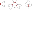
   Figure 2: (a) Linear and (b) Sicilian pants decomposition of $\mathbb{P}^{1}\left\backslash\left\{6\text{ points}\right\}\right.$; (c) gluing 1-punctured torus from a pair of pants.

   A (tri)fundamental example where this construction becomes important is known in the gauge theory literature under the name of Sicilian quiver (Fig. 2b). Already for $N=2$ the monodromies along the triple of internal cicles of this pants decomposition cannot be simultaneously reduced to the form “$\mathbb{1}+$rank 1 matrix” by factoring out a suitable scalar piece. The analog of expansion (4.23) in Theorem 4.6 will therefore be more intricate yet explicitly computable. Since the identification [ILTe] of the tau function of the Garnier system with a Fourier transform of $c=1$ Virasoro conformal block does not put any constraint on the employed pants decomposition, Sicilian expansion of the Garnier tau function may be used to produce an analog of Nekrasov representation for the corresponding conformal blocks. It might be interesting to compare the results obtained in this way against instanton counting [HKS].

   Extension of the procedure to higher genus requires introducing additional simple (diagonal in the Fourier basis) operators acting on some of the internal annuli. They give rise to a part of moduli of complex structure of the Riemann surface and correspond to gluing a handle out of two boundary components. Fig. 2c shows how a 1-punctured torus may be obtained by gluing two boundary circles of a pair of pants. The gluing operator encodes the elliptic modulus, which plays a role of the time variable in the corresponding isomonodromic problem. Elliptic isomonodromic deformations have been studied e.g. in [Kor], where the interested reader can find further references.

3. It is natural to wonder to what extent the approach proposed in the present work may be followed in the presence of irregular singularities, in particular, for Painlev I–V equations. The contours of appropriate isomonodromic RHPs become more complicated: in addition to circles of formal monodromy, they include anti-Stokes rays, exponential jumps on which account for Stokes phenomenon [FIKN]. We will sketch here a partial answer in rank $N=2$. For this it is useful to recall a geometric representation of the confluence diagram for Painlev equations recently proposed by Chekhov, Mazzocco and Rubtsov [CM, CMR], see Fig. 3. To each of the equations (or rather associated linear problems) is assigned a Riemann surface with a number of cusped boundary components. They are obtained from Painlev VI 4-holed sphere using two surgery operations: i) a “chewing-gum” move creating from two holes with $k$ and $l$ cusps one hole with $k+l+2$ cusps and ii) a cusp removal reducing the number of cusps at one hole by $1$. The cusps may be thought of as representing the anti-Stokes rays of the Riemann-Hilbert contour.

   
   

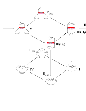
   Figure 3: CMR confluence diagram for Painlev equations.

   An extension of our approach is straightforward for equations from the upper part of the CMR diagram and, more generally, when the Poincar ranks of all irregular singular points are either $\frac{1}{2}$ or $1$. The associated surfaces may be decomposed into irregular pants of three types corresponding to solvable RHPs: Gauss hypergeometric, Whittaker and Bessel systems (Fig. 4). They serve to construct local Riemann-Hilbert parametrices which in turn produce the relevant Plemelj operators.

   

   Figure 4: Some solvable RHPs in rank $N=2$: Gauss hypergeometric (3 regular punctures), Whittaker (1 regular + 1 of Poincar rank 1) and Bessel (1 regular + 1 of rank $\frac{1}{2}$).

   The study of higher Poincar rank seems to require new ideas. Moreover, even for Painlev V and Painlev  III Fredholm determinant expansions naturally give series representations of the corresponding tau functions of regular type, first proposed in [GIL13] and expressed in terms of irregular conformal blocks of [G, BMT, GT]. It is not clear to us how to extract from them irregular (long-distance) asymptotic expansions. Let us mention a recent work [Nag] which relates such expansions to irregular conformal blocks of a different type.

4. Given a matrix $K\in\mathbb{C}^{\mathfrak{X}\times\mathfrak{X}}$ indexed by elements of a discrete set $\mathfrak{X}$, it is almost a tautology to say that the principal minors $\operatorname{det}K_{\mathfrak{Y}\in 2^{\mathfrak{X}}}$ define a determinantal point process on $\mathfrak{X}$ and a probability measure on $2^{\mathfrak{X}}$. Fredholm determinant representations and combinatorial expansions of tau functions thus generalize in a natural way various families of measures of random matrix or representation-theoretic origin, such as $Z$- and $ZW$-measures [BO1, BO2] (the former correspond to the scalar case $N=1$ with $n=4$ regular singular points, and the latter are related to hypergeometric kernel considered in the last subsection). We believe that novel probabilistic models coming from isomonodromy deserve further investigation.

5. Perhaps the most intriguing perspective is to extend our setup to $q$-isomonodromy problems, in particular $q$-difference Painlevé equations, presumably related to the deformed Virasoro algebra [SKAO] and 5D gauge theories. Among the results pointing in this direction, let us mention a study of the connection problem for $q$-Painlevé VI [Ma] based on asymptotic factorization of the associated linear problem into two systems solved by the Heine basic hypergeometric series ${}_{2}\varphi_{1}$, and critical expansions for solultions of $q$-$P\left(A_{1}\right)$ equation recently obtained in [JR].

Acknowledgements. We would like to thank F. Balogh, M. Bershtein, M. Bertola, A. Bufetov, M. Cafasso, T. Grava, J. Harnad, G. Helminck, N. Iorgov, A. Its, A. Marshakov, H. Nagoya, V. Poberezhny and V. Rubtsov for their interest to this project and useful discussions. The present work was supported by the CNRS/PICS project “Isomonodromic deformations and conformal field theory”. P. G. was supported by the RSF grant No. 16-11-10160 (results of Section 4), the Russian Academic Excellence Project ’5-100’, and the “Young Russian Mathematics” fellowship. P. G. would also like to thank KdV Institute of the University of Amsterdam, where a part of this work was done, and especially G. Helminck, for warm hospitality.

2 Tau functions as Fredholm determinants

2.1 Riemann-Hilbert setup

The classical setting of the Riemann-Hilbert problem (RHP) involves two basic ingredients: • A contour $\Gamma$ on a Riemann surface $\Sigma$ of genus $g$ consisting of a finite set of smooth oriented arcs that can intersect transversally. Orientation of the arcs defines positive and negative side $\Gamma_{\pm}$ of the contour in the usual way, see Fig. 5. • A jump matrix $J:\Gamma\to\mathrm{GL}\left(N,\mathbb{C}\right)$ that satisfies suitable smoothness requirements. Figure 5: Orientation and                                                                                                                                          labeling of sides of $\Gamma$

The RHP defined by the pair $\left(\Gamma,J\right)$ consists in finding an analytic invertible matrix function $\Psi:\Sigma\backslash\Gamma\to\mathrm{GL}\left(N,\mathbb{C}\right)$ whose boundary values $\Psi_{\pm}$ on $\Gamma_{\pm}$ are related by $\Psi_{+}=J\Psi_{-}$. Uniqueness of the solution is ensured by adding an appropriate normalization condition.

In the present work we are mainly interested in the genus $0$ case: $\Sigma=\mathbb{P}^{1}$. Let us fix a collection

$$a:=\left(a_{0}=0,a_{1},\ldots,a_{n-3},a_{n-2}=1,a_{n-1}=\infty\right)$$

of $n$ distinct points on $\mathbb{P}^{1}$ satisfying the condition of radial ordering $0<|a_{1}|<\ldots<|a_{n-3}|<1$. To reduce the amount of fuss below, it is convenient to assume that $a_{1},\ldots,a_{n-3}\in\mathbb{R}_{>0}$. The contour $\Gamma$ will then be chosen as a collection

$$\Gamma=\bigl{(}\bigcup\nolimits_{k=0}^{n-1}\gamma_{k}\Bigr{)}\cup\bigl{(}\bigcup\nolimits_{k=0}^{n-2}\ell_{k}\Bigr{)}$$

of counter-clockwise oriented circles $\gamma_{k}$ of sufficiently small radii centered at $a_{k}$, and the segments $\ell_{k}\subset\mathbb{R}$ joining the circles $\gamma_{k}$ and $\gamma_{k+1}$, see Fig. 6.

Figure 6: Contour $\Gamma$ for $n=5$

The jumps will be defined by the following data:

• An $n$-tuple of diagonal $N\times N$ matrices $\Theta_{k}=\operatorname{diag}\left\{\theta_{k,1},\ldots,\theta_{k,N}\right\}\in\mathbb{C}^{N\times N}$ (with $k=0,\ldots,n-1$) satisfying Fuchs consistency relation $\sum_{k=0}^{n-1}\operatorname{Tr}\Theta_{k}=0$ and having non-resonant spectra. The latter condition means that ${\theta_{k,\alpha}-\theta_{k,\beta}\notin\mathbb{Z}\backslash\left\{0\right\}}$.

• A collection of $2n$ matrices $C_{k,\pm}\in\mathrm{GL}\left(N,\mathbb{C}\right)$ subject to the constraints

  $$\begin{gathered}M_{0\to k}:=C_{k,-}e^{2\pi i\Theta_{k}}C_{k,+}^{-1}=C_{k+1,-}C_{k+1,+}^{-1},\qquad k=0,\ldots,n-3,\\ M_{0\to n-2}:=C_{n-2,-}e^{2\pi i\Theta_{n-2}}C_{n-2,+}^{-1}=C_{n-1,-}e^{-2\pi i\Theta_{n-1}}C_{n-1,+}^{-1},\\ M_{0\to n-1}:=\mathbb{1}=C_{n-1,-}C_{n-1,+}^{-1}=C_{0,-}C_{0,+}^{-1},\end{gathered}$$ (2.1)

  which are simultaneously viewed as the definition of $M_{0\to k}\in\mathrm{GL}\left(N,\mathbb{C}\right)$. Only $n$ of the initial matrices (for example, $C_{k,+}$) are therefore independent.

The jump matrix $J$ that we are going to consider is then given by

$$\begin{gathered}\begin{aligned} J\left(z\right)\Bigl{|}_{\ell_{k}}=M_{0\to k}^{\;-1},\qquad&k=0,\ldots,n-2,\\ J\left(z\right)\Bigl{|}_{\gamma_{k}}=\left(a_{k}-z\right)^{-\Theta_{k}}C_{k,\pm}^{-1},\qquad&\Im z\gtrless 0,\quad k=0,\ldots,n-2,\\ J\left(z\right)\Bigl{|}_{\gamma_{n-1}}=\left(-z\right)^{\Theta_{n-1}}C_{n-1,\pm}^{-1},\qquad&\Im z\gtrless 0.\end{aligned}\end{gathered}$$ (2.2)

Throughout this paper, complex powers will always be understood as $z^{\theta}=e^{\theta\ln z}$, the logarithm being defined on the principal branch. The subscripts $\pm$ of $C_{k,\pm}$ are sometimes omitted to lighten the notation.

A major incentive to study the above RHP comes from its direct connection to systems of linear ODEs with rational coefficients. Indeed, define a new matrix $\Phi$ by

$$\Phi\left(z\right)=\begin{cases}\Psi\left(z\right),\qquad&z\text{ outside }\gamma_{0\ldots n-1},\\ C_{k}\left(a_{k}-z\right)^{\Theta_{k}}\Psi\left(z\right),\qquad&z\text{ inside }\gamma_{k},\quad k=0,\ldots,n-2,\\ C_{n-1}\left(-z\right)^{-\Theta_{n-1}}\Psi\left(z\right),\qquad&z\text{ inside }\gamma_{n-1}.\end{cases}$$ (2.3)

It has only piecewise constant jumps $J_{\Phi}\left(z\right)\bigl{|}_{]a_{k},a_{k+1}[}=M_{0\to k}^{-1}$ on the positive real axis. The matrix $A\left(z\right):=\Phi^{-1}\partial_{z}\Phi$ is therefore meromorphic on $\mathbb{P}^{1}$ with poles only possible at $a_{0},\ldots,a_{n-1}$. It follows immediately that

$$\partial_{z}\Phi=\Phi A\left(z\right),\qquad A\left(z\right)=\sum_{k=0}^{n-2}\frac{A_{k}}{z-a_{k}},$$ (2.4)

with $A_{k}=\Psi\left(a_{k}\right)^{-1}\Theta_{k}\Psi\left(a_{k}\right)$. Thus $\Phi\left(z\right)$ is a fundamental matrix solution for a class of Fuchsian systems related by constant gauge transformations. It has prescribed monodromy and singular behavior that are encoded in the connection matrices $C_{k}$ and local monodromy exponents $\Theta_{k}$. The freedom in the choice of the gauge reflects the dependence on the normalization of $\Psi$. Let us note that the conditions (2.1) on the Riemann-Hilbert data are in fact designed with the aim to reproduce the monodromy of $\Phi\left(z\right)$. This explains a rather non-obvious fact of the absence of monodromy around the nod points of $\Gamma$, which in its turn ensures that the RHP solution does not have singularities at these points.

The monodromy representation $\rho:\pi_{1}\left(\mathbb{P}^{1}\backslash a\right)\to\mathrm{GL}\left(N,\mathbb{C}\right)$ associated to $\Phi$ is uniquely determined by the jumps. It is generated by the matrices $M_{k}=\rho\left(\xi_{k}\right)$ assigned to counter-clockwise loops $\xi_{0},\ldots,\xi_{n-1}$ represented in Fig. 7. They are obtained from $\left[T_{\xi_{k}}\left(\Phi\right)\right]\left(z\right)=M_{k}\Phi\left(z\right)$, where $T_{\xi_{k}}$ denotes the operator of analytic continuation along the loop $\xi_{k}$. These matrices may be expressed as

$$M_{0}=M_{0\to 0},\qquad M_{k+1}={M_{0\to k}}^{-1}M_{0\to k+1},$$

which means simply that $M_{0\to k}=M_{0}\ldots M_{k-1}M_{k}$. It is a direct consequence of the definition (2.1) that the spectra of $M_{k}$ coincide with those of $e^{2\pi i\Theta_{k}}$. In fact, $M_{k}=C_{k,+}e^{2\pi i\Theta_{k}}C_{k,+}^{-1}$.

Figure 7: Generators of $\pi_{1}\left(\mathbb{P}^{1}\backslash a\right)$

Assumption 2.1.

The matrices $M_{0\to k}$ with $k=1,\ldots,n-3$ are assumed to be diagonalizable:

$$M_{0\to k}=S_{k}e^{2\pi i\mathfrak{S}_{k}}S_{k}^{-1},\qquad\mathfrak{S}_{k}=\operatorname{diag}\left\{\sigma_{k,1},\ldots,\sigma_{k,N}\right\}.$$

It can then be assumed without loss in generality that $\operatorname{Tr}\mathfrak{S}_{k}=\sum_{j=0}^{k}\operatorname{Tr}\,\Theta_{j}$ and $\left|\Re\left(\sigma_{k,\alpha}-\sigma_{k,\beta}\right)\right|\leq 1$. We further impose a non-resonancy condition $\sigma_{k,\alpha}-\sigma_{k,\beta}\neq\pm 1$.

In order to have uniform notation, we may also identify $\mathfrak{S}_{0}\equiv\Theta_{0}$, $\mathfrak{S}_{n-2}\equiv-\Theta_{n-1}$. Note that any sufficiently generic monodromy representation can be realized as described above.

2.2 Auxiliary $3$-point RHPs

Consider a decomposition of the original $n$-punctured sphere into $n-2$ pairs of pants $\mathcal{T}^{[1]},\ldots,\mathcal{T}^{[n-2]}$ by $n-3$ annuli $\mathcal{A}_{1},\ldots,\mathcal{A}_{n-3}$ represented in Fig. 8. The labeling is designed so that two boundary components of the annulus $\mathcal{A}_{k}$ that belong to trinions $\mathcal{T}^{[k]}$ and $\mathcal{T}^{[k+1]}$ are denoted by $\mathcal{C}^{[k]}_{\text{out}}$ and $\mathcal{C}^{[k+1]}_{\text{in}}$. We are now going to associate to the $n$-point RHP described above $n-2$ simpler $3$-point RHPs assigned to different trinions and defined by the pairs $\left(\Gamma^{[k]},J^{[k]}\right)$ with $k=1,\ldots,n-2$.

Figure 8: Labeling of trinions, annuli and boundary curves

The curves $\mathcal{C}^{[k]}_{\text{in}}$ and $\mathcal{C}^{[k]}_{\text{out}}$ are represented by circles of positive and negative orientation as shown in Fig. 9. For $k=2,\ldots,n-3$, the contour $\Gamma^{[k]}$ of the RHP assigned to trinion $\mathcal{T}^{[k]}$ consists of three circles $\mathcal{C}^{[k]}_{\text{in}}$, $\mathcal{C}^{[k]}_{\text{out}}$, $\gamma_{k}$ associated to boundary components, and two segments of the real axis. For leftmost and rightmost trinions $\mathcal{T}^{[1]}$ and $\mathcal{T}^{[n-2]}$, the role of $\mathcal{C}^{[1]}_{\text{in}}$ and $\mathcal{C}^{[n-2]}_{\text{out}}$ is played respectively by the circles $\gamma_{0}$ and $\gamma_{n-1}$ around $0$ and $\infty$.

Figure 9: Contour $\Gamma^{[k]}$ (left) and $\hat{\Gamma}$ for $n=5$ (right)

The jump matrix $J^{[k]}$ is constructed according to two basic rules:

• The arcs that belong to original contour give rise to the same jumps: $\left(J^{[k]}-J\right)\bigl{|}_{\Gamma^{[k]}\cap\Gamma}=0$.

• The jumps on the boundary circles $\mathcal{C}^{[k]}_{\text{out}}$, $\mathcal{C}^{[k+1]}_{\text{in}}$ mimic regular singularities characterized by counter-clockwise monodromy matrices $M_{0\to k}$:

  $$J^{[k]}\Bigl{|}_{\mathcal{C}_{\text{out}}^{[k]}}=\left(-z\right)^{-\mathfrak{S}_{k}}S_{k}^{-1},\qquad J^{[k+1]}\Bigl{|}_{\mathcal{C}_{\text{in}}^{[k+1]}}=\left(-z\right)^{-\mathfrak{S}_{k}}S_{k}^{-1},\qquad k=1,\ldots,n-3.$$ (2.5)

The solution $\Psi^{[k]}$ of the RHP defined by the pair $\left(\Gamma^{[k]},J^{[k]}\right)$ is thus related in a way analogous to (2.3) to the fundamental matrix solution $\Phi^{[k]}$ of a Fuchsian system with 3 regular singular points at $0$, $a_{k}$ and $\infty$ characterized by monodromies $M_{0\to k-1}$, $M_{k}$, $M_{0\to k}^{-1}$:

$$\partial_{z}\Phi^{[k]}=\Phi^{[k]}A^{[k]}\left(z\right),\qquad A^{[k]}\left(z\right)=\frac{A^{[k]}_{0}}{z}+\frac{A^{[k]}_{1}}{z-a_{k}}.$$ (2.6)

We note in passing that the spectra of $A^{[k]}_{0}$, $A^{[k]}_{1}$ and $A^{[k]}_{\infty}:=-A^{[k]}_{0}-A^{[k]}_{1}$ coincide with the spectra of $\mathfrak{S}_{k-1}$, $\Theta_{k}$ and $-\mathfrak{S}_{k}$. We also assume that the monodromy is sufficiently generic so that the $3$-point Fuchsian systems with the local exponents of the fundamental solution leading to the jumps (2.5) in $\Psi^{[k]}$ exist for all $k=1,\ldots,n-2$.

It will be convenient to replace the $n$-point RHP described in the previous subsection by a slightly modified one. It is defined by a pair $\left(\hat{\Gamma},\hat{J}\right)$ such that (cf right part of Fig. 9)

$$\hat{\Gamma}=\bigcup_{k=1}^{n-2}\Gamma^{[k]},\qquad\hat{J}\Bigl{|}_{\Gamma^{[k]}}=J^{[k]}.$$ (2.7)

Constructing the solution $\hat{\Psi}$ of this RHP is equivalent to finding $\Psi$: it is plain that

$$\hat{\Psi}\left(z\right)=\begin{cases}\left(-z\right)^{-\mathfrak{S}_{k}}S_{k}^{-1}\Psi\left(z\right),\qquad&z\in\mathcal{A}_{k},\\ \Psi\left(z\right),\qquad&z\in\mathbb{P}^{1}\backslash\bigcup\limits_{k=1}^{n-3}\mathcal{A}_{k}.\end{cases}$$ (2.8)

Our aim in the next subsections is to construct the isomonodromic tau function in terms of $3$-point solutions $\Phi^{[k]}$. This construction employs in a crucial way integral Plemelj operators acting on spaces of holomorphic functions on $\mathcal{A}:=\bigcup_{k=1}^{n-3}\mathcal{A}_{k}$.

2.3 Plemelj operators

Given a positively oriented circle $\mathcal{C}\subset\mathbb{C}$ centered at the origin, let us denote by $\mathcal{V}\left(\mathcal{C}\right)$ the space of functions holomorphic in an annulus containing $\mathcal{C}$. Any $f\in\mathcal{V}\left(\mathcal{C}\right)$ is canonically decomposed as $f=f_{+}+f_{-}$, where $f_{+}$ and $f_{-}$ denote the analytic and principal part of $f$. Let us accordingly write $\mathcal{V}\left(\mathcal{C}\right)=\mathcal{V}_{+}\left(\mathcal{C}\right)\oplus\mathcal{V}_{-}\left(\mathcal{C}\right)$ and denote by $\Pi_{\pm}\left(\mathcal{C}\right)$ the projectors on the corresponding subspaces. Their explicit form is

$$\Pi_{\pm}\left(\mathcal{C}\right)f\left(z\right)=\frac{1}{2\pi i}\oint_{\mathcal{C}_{\pm},|z^{\prime}|=|z|\pm 0}\frac{f\left(z^{\prime}\right)dz^{\prime}}{z^{\prime}-z},$$

where the subscript of $\mathcal{C}_{\pm}$ indicates the orientation of $\mathcal{C}$. Projectors $\Pi_{\pm}\left(\mathcal{C}\right)$ are the classical Cauchy operators, which are simple instances of the operators extensively used below.

Let us next associate to every trinion $\mathcal{T}^{[k]}$ with $k=2,\ldots,n-3$ the spaces of vector-valued functions

$$\mathcal{H}^{[k]}=\bigoplus_{\epsilon=\mathrm{in,out}}\left(\mathcal{H}^{[k]}_{\epsilon,+}\oplus\mathcal{H}^{[k]}_{\epsilon,-}\right),\qquad\mathcal{H}^{[k]}_{\epsilon,\pm}=\mathbb{C}^{N}\otimes\mathcal{V}_{\pm}\left(\mathcal{C}_{\epsilon}^{[k]}\right).$$

With respect to the first decomposition, it is convenient to write the elements $f^{[k]}\in\mathcal{H}^{[k]}$ as

$$f^{[k]}=\left(\begin{array}[]{c}f^{[k]}_{\mathrm{in},-}\vspace{0.1cm}\\ f^{[k]}_{\mathrm{out},+}\end{array}\right)\oplus\left(\begin{array}[]{c}f^{[k]}_{\mathrm{in},+}\vspace{0.1cm}\\ f^{[k]}_{\mathrm{out},-}\end{array}\right).$$

Here $f^{[k]}_{\mathrm{\epsilon},\pm}$ denote $N$-column vectors which represent the restrictions of analytic and principal part of $f^{[k]}$ to boundary circle $\mathcal{C}_{\mathrm{\epsilon}}^{[k]}$. Now define a Plemelj operator $\mathcal{P}^{[k]}:\mathcal{H}^{[k]}\to\mathcal{H}^{[k]}$ by

$$\mathcal{P}^{[k]}f^{[k]}\left(z\right)=\frac{1}{2\pi i}\oint_{\mathcal{C}^{[k]}_{\mathrm{in}}\cup\mathcal{C}^{[k]}_{\mathrm{out}}}\frac{\Psi^{[k]}_{+}\left(z\right){\Psi^{[k]}_{+}\left(z^{\prime}\right)}^{-1}f^{[k]}\left(z^{\prime}\right)dz^{\prime}}{z-z^{\prime}}.$$ (2.9)

The singular factors $1/\left(z-z^{\prime}\right)$ for $z,z^{\prime}\in\mathcal{C}_{\mathrm{in,out}}^{[k]}$ are interpreted with the following prescription: the contour of integration is deformed to appropriate annulus (e.g. $\mathcal{A}_{k-1}$ for $\mathcal{C}_{\mathrm{in}}^{[k]}$ and $\mathcal{A}_{k}$ for $\mathcal{C}_{\mathrm{out}}^{[k]}$) as to avoid the pole at $z^{\prime}=z$. Matrix function $\Psi^{[k]}\left(z\right)$ is a solution of the $3$-point RHP described in the previous subsection. Its normalization is irrelevant as the corresponding factor cancels out in (2.9). Let us stress once again the triviality of monodromy at the nods of $\Gamma^{[k]}$, which ensures that $\Psi^{[k]}_{+}\left(z\right)$ can be analytically continued to small annuli containing $\mathcal{C}^{[k]}_{\mathrm{out}}$ and $\mathcal{C}^{[k]}_{\mathrm{in}}$.

Lemma 2.2.

We have $\left(\mathcal{P}^{[k]}\right)^{2}=\mathcal{P}^{[k]}$ and $\operatorname{ker}\mathcal{P}^{[k]}=\mathcal{H}^{[k]}_{\mathrm{in},+}\oplus\mathcal{H}^{[k]}_{\mathrm{out},-}$. Moreover, $\mathcal{P}^{[k]}$ can be explicitly written as

$$\mathcal{P}^{[k]}:\left(\begin{array}[]{c}f^{[k]}_{\mathrm{in},-}\vspace{0.1cm}\\ f^{[k]}_{\mathrm{out},+}\end{array}\right)\oplus\left(\begin{array}[]{c}f^{[k]}_{\mathrm{in},+}\vspace{0.1cm}\\ f^{[k]}_{\mathrm{out},-}\end{array}\right)\mapsto\left(\begin{array}[]{c}f^{[k]}_{\mathrm{in},-}\vspace{0.1cm}\\ f^{[k]}_{\mathrm{out},+}\end{array}\right)\oplus\left(\begin{array}[]{rr}\mathsf{a}^{[k]}&\mathsf{b}^{[k]}\vspace{0.1cm}\\ \mathsf{c}^{[k]}&\mathsf{d}^{[k]}\end{array}\right)\left(\begin{array}[]{c}f^{[k]}_{\mathrm{in},-}\vspace{0.1cm}\\ f^{[k]}_{\mathrm{out},+}\end{array}\right),$$

where the operators $\mathsf{a}^{[k]}$, $\mathsf{b}^{[k]}$, $\mathsf{c}^{[k]}$, $\mathsf{d}^{[k]}$ are defined by

$$\left(\mathsf{a}^{[k]}g\right)\left(z\right)= \,\frac{1}{2\pi i}\oint_{\mathcal{C}_{\mathrm{in}}^{[k]}}\frac{\left[\Psi^{[k]}_{+}\left(z\right){\Psi^{[k]}_{+}\left(z^{\prime}\right)}^{-1}-\mathbb{1}\,\right]g\left(z^{\prime}\right)dz^{\prime}}{z-z^{\prime}},\qquad\qquad z\in\mathcal{C}_{\mathrm{in}}^{[k]},$$ (2.10a)

$$\left(\mathsf{b}^{[k]}g\right)\left(z\right)= \,\frac{1}{2\pi i}\oint_{\mathcal{C}_{\mathrm{out}}^{[k]}}\frac{\Psi^{[k]}_{+}\left(z\right){\Psi^{[k]}_{+}\left(z^{\prime}\right)}^{-1}g\left(z^{\prime}\right)dz^{\prime}}{z-z^{\prime}},\qquad\qquad z\in\mathcal{C}_{\mathrm{in}}^{[k]},$$ (2.10b)

$$\left(\mathsf{c}^{[k]}g\right)\left(z\right)= \,\frac{1}{2\pi i}\,\oint_{\mathcal{C}_{\mathrm{in}}^{[k]}}\;\frac{\Psi^{[k]}_{+}\left(z\right){\Psi^{[k]}_{+}\left(z^{\prime}\right)}^{-1}g\left(z^{\prime}\right)dz^{\prime}}{z-z^{\prime}},\qquad\qquad z\in\mathcal{C}_{\mathrm{out}}^{[k]},$$ (2.10c)

$$\left(\mathsf{d}^{[k]}g\right)\left(z\right)= \,\frac{1}{2\pi i}\oint_{\mathcal{C}_{\mathrm{out}}^{[k]}}\frac{\left[\Psi^{[k]}_{+}\left(z\right){\Psi^{[k]}_{+}\left(z^{\prime}\right)}^{-1}-\mathbb{1}\,\right]g\left(z^{\prime}\right)dz^{\prime}}{z-z^{\prime}},\qquad\qquad z\in\mathcal{C}_{\mathrm{out}}^{[k]}.$$ (2.10d)

Proof. Let us first prove that $\mathcal{H}^{[k]}_{\mathrm{in},+},\mathcal{H}^{[k]}_{\mathrm{out},-}\subset\operatorname{ker}\mathcal{P}^{[k]}$. This statement follows from the fact that $\Psi^{[k]}_{+}$ holomorphically extends inside $\mathcal{C}_{\mathrm{in}}^{[k]}$ and outside $\mathcal{C}_{\mathrm{out}}^{[k]}$, so that the integration contours can be shrunk to $0$ and $\infty$. To prove the projection property, decompose for example

$$\left(\mathcal{P}^{[k]}f_{\mathrm{out},+}^{[k]}\right)_{\mathrm{out}}\left(z\right)=\frac{1}{2\pi i}\oint_{\mathcal{C}^{[k]}_{\mathrm{out}}}\frac{\left[\Psi^{[k]}_{+}\left(z\right){\Psi^{[k]}_{+}\left(z^{\prime}\right)}^{-1}-\mathbb{1}\,\right]f_{\mathrm{out},+}^{[k]}\left(z^{\prime}\right)dz^{\prime}}{z-z^{\prime}}+\frac{1}{2\pi i}\oint_{\mathcal{C}^{[k]}_{\mathrm{out}},|z^{\prime}|>|z|}\frac{f_{\mathrm{out},+}^{[k]}\left(z^{\prime}\right)dz^{\prime}}{z-z^{\prime}}.$$

The first integral admits holomorphic continuation in $z$ outside $\mathcal{C}_{\mathrm{out}}^{[k]}$ thanks to nonsingular integral kernel, and leads to (2.10d), whereas the second term is obviously equal to $f^{[k]}_{\mathrm{out},+}$. The action of $\mathcal{P}^{[k]}$ on $f^{[k]}_{\mathrm{in},-}$ is computed in a similar fashion. $\square$

The leftmost and rightmost trinions $\mathcal{T}^{[1]}$ and $\mathcal{T}^{[n-2]}$ play somewhat distinguished role. Let us assign to them boundary spaces

$$\mathcal{H}^{[1]}:=\mathcal{H}^{[1]}_{\mathrm{out},+}\oplus\mathcal{H}^{[1]}_{\mathrm{out},-},\qquad\mathcal{H}^{[n-2]}:=\mathcal{H}^{[n-2]}_{\mathrm{in},+}\oplus\mathcal{H}^{[n-2]}_{\mathrm{in},-},$$

and the operators $\mathcal{P}^{[k]}:\mathcal{H}^{[k]}\to\mathcal{H}^{[k]}$ with $k=1,n-2$ defined by

$$\mathcal{P}^{[1]}f^{[1]}\left(z\right)= \,\frac{1}{2\pi i}\oint_{\mathcal{C}^{[1]}_{\mathrm{out}}}\frac{\Psi^{[1]}_{+}\left(z\right){\Psi^{[1]}_{+}\left(z^{\prime}\right)}^{-1}f^{[1]}\left(z^{\prime}\right)dz^{\prime}}{z-z^{\prime}},$$

$$\mathcal{P}^{[n-2]}f^{[n-2]}\left(z\right)= \,\frac{1}{2\pi i}\oint_{\mathcal{C}^{[n-2]}_{\mathrm{in}}}\frac{\Psi^{[n-2]}_{+}\left(z\right){\Psi^{[n-2]}_{+}\left(z^{\prime}\right)}^{-1}f^{[n-2]}\left(z^{\prime}\right)dz^{\prime}}{z-z^{\prime}}.$$

Analogously to the above, one can show that

$$\mathcal{P}^{[1]}: \,\;f^{[1]}_{\mathrm{out},+}\oplus f^{[1]}_{\mathrm{out},-}\;\;\mapsto f^{[1]}_{\mathrm{out},+}\;\oplus\mathsf{d}^{[1]}f^{[1]}_{\mathrm{out},+},$$

$$\mathcal{P}^{[n-2]}: \,f^{[n-2]}_{\mathrm{in},-}\oplus f^{[n-2]}_{\mathrm{in},+}\mapsto f^{[n-2]}_{\mathrm{in},-}\oplus\mathsf{a}^{[n-2]}f^{[n-2]}_{\mathrm{in},-},$$

where the operators $\mathsf{d}^{[1]}$, $\mathsf{a}^{[n-2]}$ are given by the same formulae (2.10a), (2.10d). Note in particular that $\mathcal{P}^{[1]}$ and $\mathcal{P}^{[n-2]}$ are projections along their kernels $\mathcal{H}^{[1]}_{\mathrm{out},-}$ and $\mathcal{H}^{[n-2]}_{\mathrm{in},+}$.

Let us next introduce the total space

$$\mathcal{H}:=\bigoplus_{k=1}^{n-2}\mathcal{H}^{[k]}.$$

It admits a splitting that will play an important role below. Namely,

$$\begin{gathered}\mathcal{H}=\mathcal{H}_{+}\oplus\mathcal{H}_{-},\\ \mathcal{H}_{\pm}:=\mathcal{H}^{[1]}_{\mathrm{out},\pm}\oplus\left(\mathcal{H}^{[2]}_{\mathrm{in},\mp}\oplus\mathcal{H}^{[2]}_{\mathrm{out},\pm}\right)\oplus\ldots\oplus\left(\mathcal{H}^{[n-3]}_{\mathrm{in},\mp}\oplus\mathcal{H}^{[n-3]}_{\mathrm{out},\pm}\right)\oplus\mathcal{H}^{[n-2]}_{\mathrm{in},\mp}.\end{gathered}$$ (2.11)

Combine the 3-point projections $\mathcal{P}^{[k]}$ into an operator $\mathcal{P}_{\oplus}:\mathcal{H}\to\mathcal{H}$ given by the direct sum

$$\mathcal{P}_{\oplus}=\mathcal{P}^{[1]}\oplus\ldots\oplus\mathcal{P}^{[n-2]}.$$

Clearly, we have

Lemma 2.3.

$\mathcal{P}_{\oplus}^{2}=\mathcal{P}_{\oplus}$ and $\operatorname{ker}\mathcal{P}_{\oplus}=\mathcal{H}_{-}$.

Another important operator $\mathcal{P}_{\Sigma}:\mathcal{H}\to\mathcal{H}$ is defined using the solution $\hat{\Psi}\left(z\right)$ (defined by (2.7)) of the $n$-point RHP in a way similar to construction of the projection (2.9):

$$\mathcal{P}_{\Sigma}f\left(z\right)=\frac{1}{2\pi i}\oint_{\mathcal{C}_{\Sigma}}\frac{\hat{\Psi}_{+}\left(z\right){\hat{\Psi}_{+}\left(z^{\prime}\right)}^{-1}f\left(z^{\prime}\right)dz^{\prime}}{z-z^{\prime}},\qquad\mathcal{C}_{\Sigma}:=\bigcup\limits_{k=1}^{n-3}\mathcal{C}^{[k]}_{\mathrm{out}}\cup\mathcal{C}_{\mathrm{in}}^{[k+1]}.$$ (2.12)

We use the same prescription for the contours: whenever it is necessary to interpret the singular factor $1/\left(z-z^{\prime}\right)$, the contour of integration is slightly deformed into the appropriate annulus.

Let $\mathcal{H}_{\mathcal{A}}$ be the space of boundary values on $\mathcal{C}_{\Sigma}$ of functions holomorphic on $\mathcal{A}=\bigcup_{k=1}^{n-3}\mathcal{A}_{k}$.

Lemma 2.4.

$\mathcal{P}_{\Sigma}^{2}=\mathcal{P}_{\Sigma}$ and $\displaystyle\mathcal{H}_{\mathcal{A}}\subseteq\operatorname{ker}\mathcal{P}_{\Sigma}$.

Proof. Given $f\in\mathcal{H}_{\mathcal{A}}$, the integration contours $\mathcal{C}_{\mathrm{out}}^{[k]}$ and $\mathcal{C}_{\mathrm{in}}^{[k+1]}$ in (2.12) can be merged thanks to the absence of singularities inside $\mathcal{A}_{k}$, which proves the second statement. To show the projection property, it suffices to notice that

$$\mathcal{P}_{\Sigma}^{2}f^{[k]}\left(z\right)=\frac{1}{\left(2\pi i\right)^{2}}\oiint_{\mathcal{C}_{\Sigma}}\frac{\hat{\Psi}_{+}\left(z\right){\hat{\Psi}_{+}\left(z^{\prime\prime}\right)}^{-1}f^{[k]}\left(z^{\prime\prime}\right)dz^{\prime}dz^{\prime\prime}}{\left(z-z^{\prime}\right)\left(z^{\prime}-z^{\prime\prime}\right)}.$$

Because of the ordering of contours prescribed above, the only obstacle to merging $\mathcal{C}_{\mathrm{out}}^{[k]}$ and $\mathcal{C}_{\mathrm{in}}^{[k]}$ in the integral with respect to $z^{\prime}$ is the pole at $z^{\prime}=z$. The result follows by residue computation. $\square$

Lemma 2.5.

$\displaystyle\mathcal{P}_{\Sigma}\mathcal{P}_{\oplus}=\mathcal{P}_{\oplus}$ and $\displaystyle\mathcal{P}_{\oplus}\mathcal{P}_{\Sigma}\mathcal{=}\mathcal{P}_{\Sigma}$.

Proof. Similar to the proof of Lemma 2.4. Use that $\hat{\Psi}^{-1}\Psi^{[k]}$ has no jumps on $\Gamma^{[k]}$ to compute by residues the intermediate integrals in $\mathcal{P}_{\Sigma}\mathcal{P}_{\oplus}$ and $\mathcal{P}_{\oplus}\mathcal{P}_{\Sigma}$. $\square$

The above suggests to introduce the notation

$$\mathcal{H}_{\mathcal{T}}:=\operatorname{im}\mathcal{P}_{\oplus}=\operatorname{im}\mathcal{P}_{\Sigma}.$$ (2.13)

The space $\mathcal{H}_{\mathcal{T}}\subset\mathcal{H}$ can be thought of as the subspace of functions on the union of boundary circles $\mathcal{C}^{[k]}_{\mathrm{in}}$, $\mathcal{C}^{[k]}_{\mathrm{out}}$ that can be continued inside $\bigcup_{k=1}^{n-2}\mathcal{T}^{[k]}$ with monodromy and singular behavior of the $n$-point fundamental matrix solution $\Phi\left(z\right)$. The only exception is the regular singularity at $\infty$ where the growth is slower.

The structure of elements of $\mathcal{H}_{\mathcal{T}}$ is described by Lemma 2.2. Varying the positions of singular points, one obtains a trajectory of $\mathcal{H}_{\mathcal{T}}$ in the infinite-dimensional Grassmannian $\mathrm{Gr}\left(\mathcal{H}\right)$ defined with respect to the splitting $\mathcal{H}=\mathcal{H}_{+}\oplus\mathcal{H}_{-}$. Note that each of the subspaces $\mathcal{H}_{\pm}$ may be identified with $N\left(n-3\right)$ copies of the space $L^{2}\left(S^{1}\right)$ of functions on a circle; the factor $n-3$ corresponds to the number of annuli and $N$ is the rank of the appropriate RHP.

We can also write

$$\mathcal{H}=\mathcal{H}_{\mathcal{T}}\oplus\mathcal{H}_{-}.$$ (2.14)

The operator $\mathcal{P}_{\oplus}$ introduced above gives the projection on $\mathcal{H}_{\mathcal{T}}$ along $\mathcal{H}_{-}$. Similarly, the operator $\mathcal{P}_{\Sigma}$ is a projection on $\mathcal{H}_{\mathcal{T}}$ along $\operatorname{ker}\mathcal{P}_{\Sigma}\supseteq\mathcal{H}_{\mathcal{A}}$. We would like to express it in terms of $3$-point projectors. To this end let us regard $f^{[k]}_{\mathrm{in},-}$, $f^{[k]}_{\mathrm{out},+}$ as coordinates on $\mathcal{H}_{\mathcal{T}}$. Suppose that $f\in\mathcal{H}$ can be decomposed as $f=g+h$ with $g\in\mathcal{H}_{\mathcal{T}}$ and $h\in\mathcal{H}_{\mathcal{A}}$. The latter condition means that

$$h^{[k]}_{\mathrm{out},\pm}=h^{[k+1]}_{\mathrm{in},\pm},\qquad k=1,\ldots,n-3,$$

which can be equivalently written as a system of equations for components of $g$:

$$\begin{gathered}\begin{aligned} g^{[k]}_{\mathrm{in},-}-\mathsf{c}^{[k-1]}g^{[k-1]}_{\mathrm{in},-}-\mathsf{d}^{[k-1]}g^{[k-1]}_{\mathrm{out},+}=&\,f^{[k]}_{\mathrm{in},-}-f^{[k-1]}_{\mathrm{out},-},\\ g^{[k]}_{\mathrm{out},+}-\mathsf{a}^{[k+1]}g^{[k+1]}_{\mathrm{in},-}-\mathsf{b}^{[k+1]}g^{[k+1]}_{\mathrm{out},+}=&\,f^{[k]}_{\mathrm{out},+}-f^{[k+1]}_{\mathrm{in},+},\end{aligned}\end{gathered}$$ (2.15)

where $g^{[1]}_{\mathrm{in},-}=0$, $g^{[n-2]}_{\mathrm{out},+}=0$. The first and second equations are valid in sufficiently narrow annuli containing $\mathcal{C}_{\mathrm{in}}^{[k]}$ and $\mathcal{C}_{\mathrm{out}}^{[k]}$, respectively. Define

$$\begin{gathered}\tilde{g}_{k}=\left(\begin{array}[]{c}g^{[k]}_{\mathrm{out},+}\\ g^{[k+1]}_{\mathrm{in},-}\end{array}\right),\qquad\tilde{f}_{k}=\left(\begin{array}[]{c}f^{[k]}_{\mathrm{out},+}-f^{[k+1]}_{\mathrm{in},+}\\ f^{[k+1]}_{\mathrm{in},-}-f^{[k]}_{\mathrm{out},-}\end{array}\right),\qquad U_{k}=\left(\begin{array}[]{cc}0&\mathsf{a}^{[k+1]}\\ \mathsf{d}^{[k]}&0\end{array}\right),\qquad k=1,\ldots,n-3,\\ V_{k}=\left(\begin{array}[]{cc}\mathsf{b}^{[k+1]}&0\\ 0&0\end{array}\right),\qquad W_{k}=\left(\begin{array}[]{cc}0&0\\ 0&\mathsf{c}^{[k+1]}\end{array}\right),\qquad k=1,\ldots,n-4,\\ K=\left(\begin{array}[]{cccccc}U_{1}&V_{1}&0&.&0\\ W_{1}&U_{2}&V_{2}&.&0\\ 0&W_{2}&U_{3}&.&.\\ .&.&.&.&V_{n-4}\\ 0&0&.&W_{n-4}&U_{n-3}\end{array}\right),\qquad\vec{g}=\left(\begin{array}[]{c}\tilde{g}_{1}\\ \tilde{g}_{2}\\ \vdots\\ \tilde{g}_{n-3}\end{array}\right),\qquad\vec{f}=\left(\begin{array}[]{c}\tilde{f}_{1}\\ \tilde{f}_{2}\\ \vdots\\ \tilde{f}_{n-3}\end{array}\right).\end{gathered}$$ (2.16)

The system (2.15) can then be rewritten in a block-tridiagonal form

$$\left(\mathbb{1}-K\right)\vec{g}=\vec{f}.$$ (2.17)

The decomposition $\mathcal{H}=\mathcal{H}_{\mathcal{T}}\oplus\mathcal{H}_{\mathcal{A}}$ thus uniquely exists provided that $\mathbb{1}-K$ is invertible.

Let us prove a converse result and interpret $K$ in a more invariant way. Consider the operators $\mathcal{P}_{\oplus,+}:\mathcal{H}_{+}\to\mathcal{H}_{\mathcal{T}}$ and ${\mathcal{P}_{\Sigma,+}:\mathcal{H}_{+}\to\mathcal{H}_{\mathcal{T}}}$ defined as restrictions of $\mathcal{P}_{\oplus}$ and $\mathcal{P}_{\Sigma}$ to $\mathcal{H}_{+}$. The first of them is invertible, with the inverse given by the projection on $\mathcal{H}_{+}$ along $\mathcal{H}_{-}$. Hence one can consider the composition $L\in\operatorname{End}\left(\mathcal{H}_{+}\right)$ defined by

$$L:={\mathcal{P}_{\oplus,+}}^{-1}\mathcal{P}_{\Sigma,+}.$$ (2.18)

We are now going to make an important assumption which is expected to hold generically (more precisely, outside the Malgrange divisor). It will soon become clear that it is satisfied at least in a sufficiently small finite polydisk $\mathbb{D}\subset\mathbb{C}^{n-3}$ in the variables $a_{1},\ldots,a_{n-3}$, centered at the origin.

Assumption 2.6.

$\mathcal{P}_{\Sigma,+}$ is invertible.

Proposition 2.7.

For $g\in\mathcal{H}_{+}$, let $\tilde{g}_{k}$ and $\vec{g}$ be defined by (2.16). In these coordinates, $L^{-1}=1-K$.

Proof. Rewrite the equation $L^{-1}f^{\prime}=f$ as $\mathcal{P}_{\oplus,+}f^{\prime}=\mathcal{P}_{\Sigma,+}f$. Setting $f=\mathcal{P}_{\oplus,+}f^{\prime}+h$, the latter equation becomes equivalent to $\mathcal{P}_{\Sigma}h=0$. The solution thus reduces to constructing $h\in\mathcal{H}_{\mathcal{A}}$ such that $\left(h+\mathcal{P}_{\oplus,+}f^{\prime}\right)_{-}=0$, where the projection is taken with respect to the splitting $\mathcal{H}=\mathcal{H}_{+}\oplus\mathcal{H}_{-}$. This can be achieved by setting

$$h^{[k]}_{\mathrm{out},+}= \,h^{[k+1]}_{\mathrm{in},+}=-\left(\mathcal{P}_{\oplus,+}f^{\prime}\right)^{[k+1]}_{\mathrm{in},+},$$

$$h^{[k]}_{\mathrm{out},-}= \,h^{[k+1]}_{\mathrm{in},-}=-\left(\mathcal{P}_{\oplus,+}f^{\prime}\right)^{[k]}_{\mathrm{out},-}.$$

It then follows that $f=f^{\prime}+h_{+}=\left(\mathbb{1}-K\right)f^{\prime}$. $\square$

Let us emphasize that the operator $L$ involves the (a priori unknown) solution $\hat{\Psi}\left(z\right)$ of the original RHP, equivalent to the solution of the $n$-point Fuchsian system, whereas $K$ is expressed solely in terms of $3$-point parametrices. It is this fact which ultimately allows us to obtain in the next subsections a Fredholm determinant representation of the tau function involving only these elementary building blocks.

2.4 Tau function

Definition 2.8.

Let $L\in\operatorname{End}\left(\mathcal{H}_{+}\right)$ be the operator defined by (2.18). We define the tau function associated to the Riemann-Hilbert problem for $\Psi$ as

$$\tau\left(a\right):=\operatorname{det}\left(L^{-1}\right).$$ (2.19)

In order to demonstrate the relation of (2.19) to conventional definition [JMU] of the isomonodromic tau function and its extension [ILP], let us compute the logarithmic derivatives of $\tau$ with respect to isomonodromic times $a_{1},\ldots,a_{n-3}$. At this point it is convenient to introduce the notation

$$\Delta_{k}=\frac{1}{2}\operatorname{Tr}\Theta_{k}^{2},\qquad\bar{\Delta}_{k}=\frac{1}{2}\operatorname{Tr}\mathfrak{S}_{k}^{2}.$$ (2.20)

Recall that $\bar{\Delta}_{0}\equiv\Delta_{0}$ and $\bar{\Delta}_{n-2}\equiv\Delta_{n-1}$.

Theorem 2.9.

We have

$$\tau\left(a\right)={\Upsilon\left(a\right)}^{-1}\tau_{\mathrm{JMU}}\left(a\right),$$ (2.21)

where $\tau_{\mathrm{JMU}}\left(a\right)$ is defined up to a constant independent of $a$ by

$$d_{a}\ln\tau_{\mathrm{JMU}}=\sum_{0\leq k<l\leq n-2}\operatorname{Tr}A_{k}A_{l}\;d\ln\left(a_{k}-a_{l}\right),$$ (2.22)

and the prefactor $\Upsilon\left(a\right)$ is given by

$$\Upsilon\left(a\right)=\prod_{k=1}^{n-3}a_{k}^{\bar{\Delta}_{k}-\bar{\Delta}_{k-1}-\Delta_{k}}.$$ (2.23)

Proof. We will proceed in several steps.
Step 1. Choose a collection of points $a^{0}$ close to $a$ in the sense that the same annuli can be used to define the tau function $\tau\left(a^{0}\right)$. The collection $a^{0}$ will be considered fixed whereas $a$ varies. Let us compute the logarithmic derivatives of the ratio $\tau\left(a\right)/\tau\left(a^{0}\right)$. First of all we can write

$$\frac{\tau\left(a\right)}{\tau\left(a^{0}\right)}=\operatorname{det}\left({\mathcal{P}_{\oplus,+}\left(a^{0}\right)}^{-1}\mathcal{P}_{\Sigma,+}\left(a^{0}\right){\mathcal{P}_{\Sigma,+}\left(a\right)}^{-1}\mathcal{P}_{\oplus,+}\left(a\right)\right)$$ (2.24)

Note that since $\mathcal{P}_{\Sigma,+}\left(a\right):\mathcal{H}_{+}\to\mathcal{H}_{\mathcal{T}}\left(a\right)$ can be viewed as a projection of elements of $\mathcal{H}$ along $\mathcal{H}_{\mathcal{A}}$, the composition

$$\mathcal{P}_{a^{0}\to a}:=\mathcal{P}_{\Sigma,+}\left(a\right){\mathcal{P}_{\Sigma,+}\left(a^{0}\right)}^{-1}:\mathcal{H}_{\mathcal{T}}\left(a^{0}\right)\to\mathcal{H}_{\mathcal{T}}\left(a\right)$$

is also a projection along $\mathcal{H}_{\mathcal{A}}$. It therefore coincides with the restriction $\mathcal{P}_{\Sigma}\bigl{|}_{\mathcal{H}_{\mathcal{T}}\left(a^{0}\right)}$. One similarly shows that

$$\mathcal{F}_{a^{0}\to a}:=\mathcal{P}_{\oplus,+}\left(a\right){\mathcal{P}_{\oplus,+}\left(a^{0}\right)}^{-1}=\mathcal{P}_{\oplus}\bigl{|}_{\mathcal{H}_{\mathcal{T}}\left(a^{0}\right)}.$$

The exterior logarithmic derivative of (2.24) can now be written as

$$d_{a}\ln\frac{\tau\left(a\right)}{\tau\left(a^{0}\right)}= \,-\operatorname{Tr}_{\mathcal{H}_{\mathcal{T}}\left(a^{0}\right)}\biggl{\{}d_{a}\left(\mathcal{F}_{a\to a^{0}}\mathcal{P}_{a^{0}\to a}\right)\cdot\mathcal{P}_{a\to a^{0}}\mathcal{F}_{a^{0}\to a}\biggr{\}}=$$

$$= \,-\operatorname{Tr}_{\mathcal{H}_{\mathcal{T}}\left(a^{0}\right)}\biggl{\{}\mathcal{F}_{a\to a^{0}}\cdot d_{a}\mathcal{P}_{a^{0}\to a}\cdot\mathcal{P}_{a\to a^{0}}\mathcal{F}_{a^{0}\to a}\biggr{\}}=$$ (2.25)

$$= \,-\operatorname{Tr}_{\mathcal{H}}\biggl{\{}\mathcal{P}_{\oplus}\left(a^{0}\right)\cdot d_{a}\mathcal{P}_{\Sigma}\left(a\right)\cdot\mathcal{P}_{\Sigma}\left(a^{0}\right)\mathcal{P}_{\oplus}\left(a\right)\biggr{\}}.$$

The possibility to extend operator domains as to have the second equality is a consequence of (2.13). Furthermore, using once again the projection properties, one shows that

$$\mathcal{P}_{\Sigma}\left(a\right)\Bigl{(}\mathbb{1}-\mathcal{P}_{\Sigma}\left(a^{0}\right)\Bigr{)}=0,\qquad\mathcal{P}_{\oplus}\left(a\right)\Bigl{(}\mathbb{1}-\mathcal{P}_{\oplus}\left(a^{0}\right)\Bigr{)}=0.$$

which reduces the equation (2.25) to

$$d_{a}\ln\tau\left(a\right)=-\operatorname{Tr}_{\mathcal{H}}\biggl{\{}\mathcal{P}_{\oplus}d_{a}\mathcal{P}_{\Sigma}\biggr{\}}=-\sum_{k=1}^{n-2}\operatorname{Tr}_{\mathcal{H}^{[k]}}\biggl{\{}\mathcal{P}_{\oplus}^{[k]}d_{a}\mathcal{P}_{\Sigma}\biggr{\}}.$$ (2.26)

Step 2. Let us now proceed to calculation of the right side of (2.26). Computations of the same type have already been used in the proofs of Lemmata 2.4 and 2.5. The idea is that $\Psi^{[k]}$ and $\hat{\Psi}$ have the same jumps on the contour $\Gamma^{[k]}$ which reduces the integrals in (2.9), (2.12) to residue computation. In particular, for $f^{[k]}\in\mathcal{H}^{[k]}$ with $k=2,\ldots,n-3$ we have

$$\mathcal{P}_{\oplus}^{[k]}d_{a}\mathcal{P}_{\Sigma}f^{[k]}\left(z\right)=\frac{1}{\left(2\pi i\right)^{2}}\oiint_{\mathcal{C}_{\mathrm{in}}^{[k]}\cup\mathcal{C}_{\mathrm{out}}^{[k]}}\frac{\Psi_{+}^{[k]}\left(z\right){\Psi_{+}^{[k]}\left(z^{\prime}\right)}^{-1}d_{a}\left(\hat{\Psi}_{+}\left(z^{\prime}\right){\hat{\Psi}_{+}\left(z^{\prime\prime}\right)}^{-1}\right)f^{[k]}\left(z^{\prime\prime}\right)dz^{\prime}dz^{\prime\prime}}{\left(z-z^{\prime}\right)\left(z^{\prime}-z^{\prime\prime}\right)}.$$ (2.27)

The integrals are computed with the prescription that $z$ is located inside the contour of $z^{\prime}$, itself located inside the contour of $z^{\prime\prime}$, and then passing to boundary values. But since the function $\left(z^{\prime}-z^{\prime\prime}\right)^{-1}d_{a}\left(\hat{\Psi}_{+}\left(z^{\prime}\right){\hat{\Psi}_{+}\left(z^{\prime\prime}\right)}^{-1}\right)$ has no singularity at $z^{\prime\prime}=z^{\prime}$, the contours of $z^{\prime}$ and $z^{\prime\prime}$ can be moved through each other. This identifies the trace of the integral operator on the right of (2.27) with

$$\operatorname{Tr}\left(\mathcal{P}_{\oplus}^{[k]}d_{a}\mathcal{P}_{\Sigma}\right)= \,-\frac{1}{\left(2\pi i\right)^{2}}\oiint_{\mathcal{C}_{\mathrm{in}}^{[k]}\cup\mathcal{C}_{\mathrm{out}}^{[k]}}\frac{\operatorname{Tr}\left\{{\Psi_{+}^{[k]}\left(z\right)\Psi_{+}^{[k]}\left(z^{\prime}\right)}^{-1}d_{a}\left(\hat{\Psi}_{+}\left(z^{\prime}\right){\hat{\Psi}_{+}\left(z\right)}^{-1}\right)\right\}dz\,dz^{\prime}}{\left(z-z^{\prime}\right)^{2}}=$$

$$= \,-\frac{1}{\left(2\pi i\right)^{2}}\oiint_{\mathcal{C}_{\mathrm{in}}^{[k]}\cup\mathcal{C}_{\mathrm{out}}^{[k]}}\frac{\operatorname{Tr}\left\{{\Psi_{+}^{[k]}\left(z^{\prime}\right)}^{-1}d_{a}\hat{\Psi}_{+}\left(z^{\prime}\right)\cdot{\hat{\Psi}_{+}\left(z\right)}^{-1}\Psi_{+}^{[k]}\left(z\right)\right\}dz\,dz^{\prime}}{\left(z-z^{\prime}\right)^{2}}$$

$$\,-\frac{1}{\left(2\pi i\right)^{2}}\oiint_{\mathcal{C}_{\mathrm{in}}^{[k]}\cup\mathcal{C}_{\mathrm{out}}^{[k]}}\frac{\operatorname{Tr}\left\{d_{a}\left({\hat{\Psi}_{+}\left(z\right)}^{-1}\right)\cdot\Psi_{+}^{[k]}\left(z\right){\Psi_{+}^{[k]}\left(z^{\prime}\right)}^{-1}\hat{\Psi}_{+}\left(z^{\prime}\right)\right\}dz\,dz^{\prime}}{\left(z-z^{\prime}\right)^{2}},$$

where $z$ is considered to be inside the contour of $z^{\prime}$. The first term vanishes since the contours $\mathcal{C}_{\mathrm{in}}^{[k]}$ and $\mathcal{C}_{\mathrm{out}}^{[k]}$ in the integral with respect to $z$ can be merged. In the second term the integral with respect to $z^{\prime}$ is determined by the residue at $z^{\prime}=z$, which yields

$$\operatorname{Tr}\left(\mathcal{P}_{\oplus}^{[k]}d_{a}\mathcal{P}_{\Sigma}\right)=\frac{1}{2\pi i}\oint_{\mathcal{C}_{\mathrm{in}}^{[k]}\cup\mathcal{C}_{\mathrm{out}}^{[k]}}\operatorname{Tr}\left\{d_{a}\left({\hat{\Psi}_{+}\left(z\right)}^{-1}\right)\cdot\Psi_{+}^{[k]}\left(z\right)\cdot\partial_{z}\left({\Psi_{+}^{[k]}\left(z\right)}^{-1}\hat{\Psi}_{+}\left(z\right)\right)\right\}dz.$$

Recall that $\hat{\Psi}_{+}$, $\Psi^{[k]}_{+}$ are related to fundamental matrix solutions $\Phi$, $\Phi^{[k]}$ of $n$-point and $3$-point Fuchsian systems by

$$\begin{gathered}\hat{\Psi}_{+}\left(z\right)\Bigl{|}_{\mathcal{C}_{\mathrm{in}}^{[k]}}=S_{k-1}^{-1}\left(-z\right)^{-\mathfrak{S}_{k-1}}\Phi\left(z\right),\qquad\hat{\Psi}_{+}\left(z\right)\Bigl{|}_{\mathcal{C}_{\mathrm{out}}^{[k]}}=S_{k}^{-1}\left(-z\right)^{-\mathfrak{S}_{k}}\Phi\left(z\right),\\ \Psi_{+}^{[k]}\left(z\right)\Bigl{|}_{\mathcal{C}_{\mathrm{in}}^{[k]}}=S_{k-1}^{-1}\left(-z\right)^{-\mathfrak{S}_{k-1}}\Phi^{[k]}\left(z\right),\qquad\Psi_{+}^{[k]}\left(z\right)\Bigl{|}_{\mathcal{C}_{\mathrm{out}}^{[k]}}=S_{k}^{-1}\left(-z\right)^{-\mathfrak{S}_{k}}\Phi^{[k]}\left(z\right).\end{gathered}$$

This leads to

$$\operatorname{Tr}\left(\mathcal{P}_{\oplus}^{[k]}d_{a}\mathcal{P}_{\Sigma}\right)= \,\frac{1}{2\pi i}\oint_{\mathcal{C}_{\mathrm{in}}^{[k]}\cup\mathcal{C}_{\mathrm{out}}^{[k]}}\operatorname{Tr}\left\{d_{a}\left({\Phi}^{-1}\right)\cdot\Phi^{[k]}\cdot\partial_{z}\left({\Phi^{[k]}}^{-1}\Phi\right)\right\}dz=$$

$$= \,\operatorname{res}_{z=a_{k}}\operatorname{Tr}\left\{d_{a}\Phi\cdot\Phi^{-1}\left(\partial_{z}\Phi\cdot\Phi^{-1}-\partial_{z}\Phi^{[k]}\cdot{\Phi^{[k]}}^{-1}\right)\right\}.$$ (2.28)

The contributions of the subspaces $\mathcal{H}^{[1]}$ and $\mathcal{H}^{[n-2]}$ to the trace (2.26) can be computed in a similar fashion. The only difference is that instead of merging $\mathcal{C}_{\mathrm{in}}^{[k]}$ with $\mathcal{C}_{\mathrm{out}}^{[k]}$ one should now shrink the contour $\mathcal{C}_{\mathrm{out}}^{[1]}$ to $0$ and $\mathcal{C}_{\mathrm{in}}^{[n-2]}$ to $\infty$. The result is given by the same formula (2.28).
Step 3. To complete the proof, it now remains to compute the residues in (2.28). Note that near the regular singularity $z=a_{k}$ the fundamental matrices $\Phi$, $\Phi^{[k]}$ are characterized by the behavior

$$\Phi\left(z\to a_{k}\right)= \,C_{k}\left(a_{k}-z\right)^{\Theta_{k}}\left(\mathbb{1}+\sum_{l=1}^{\infty}g_{k,l}\left(z-a_{k}\right)^{l}\right)G_{k},$$ (2.29a)

$$\Phi^{[k]}\left(z\to a_{k}\right)= \,C_{k}\left(a_{k}-z\right)^{\Theta_{k}}\left(\mathbb{1}+\sum_{l=1}^{\infty}g^{[k]}_{1,l}\left(z-a_{k}\right)^{l}\right)G^{[k]}_{1}.$$ (2.29b)

The coinciding leftmost factors ensure the same local monodromy properties. The rightmost coefficients appear in the $n$-point and $3$-point RHPs as $G_{k}=\Psi\left(a_{k}\right)$, $G_{1}^{[k]}=\Psi^{[k]}\left(a_{k}\right)$. It becomes straightforward to verify that as $z\to a_{k}$, one has

$$\partial_{z}\Phi\cdot\Phi^{-1}-\partial_{z}\Phi^{[k]}\cdot{\Phi^{[k]}}^{-1}= \,C_{k}\left(a_{k}-z\right)^{\Theta_{k}}\Bigl{[}g_{k,1}-g^{[k]}_{1,1}+O\left(z-a_{k}\right)\Bigr{]}\left(a_{k}-z\right)^{-\Theta_{k}}C_{k}^{-1},$$

$$d_{a}\Phi\cdot\Phi^{-1}= \,C_{k}\left(a_{k}-z\right)^{\Theta_{k}}\left[-\frac{\Theta_{k}da_{k}}{z-a_{k}}+O\left(1\right)\right]\left(a_{k}-z\right)^{-\Theta_{k}}C_{k}^{-1}.$$

In combination with (2.26), (2.28), this in turn implies that

$$d_{a}\ln\tau\left(a\right)=\sum_{k=1}^{n-3}\operatorname{Tr}\Theta_{k}\left(g_{k,1}-g^{[k]}_{1,1}\right)da_{k}.$$ (2.30)

Substituting local expansion (2.29a) into the Fuchsian system (2.4), we may recursively determine the coefficients $g_{k,l}$. In particular, the first coefficient $g_{k,1}$ satisfies

$$g_{k,1}+\left[\Theta_{k},g_{k,1}\right]=G_{k}^{-1}\left(\sum^{n-2}_{l=0,l\neq k}\frac{A_{l}}{a_{k}-a_{l}}\right)G_{k},$$ (2.31)

so that

$$\sum_{k=1}^{n-3}\operatorname{Tr}\left(\Theta_{k}g_{k,1}\right)da_{k}=\sum_{k=1}^{n-3}\sum^{n-2}_{l=0,l\neq k}\frac{\operatorname{Tr}A_{k}A_{l}}{a_{k}-a_{l}}da_{k}=d_{a}\ln\tau_{\mathrm{JMU}}.$$ (2.32)

The $3$-point analog of the relation (2.31) is

$$g^{[k]}_{1,1}+\left[\Theta_{k},g^{[k]}_{1,1}\right]={G_{1}^{[k]}}\frac{A_{0}^{[k]}}{a_{k}}{G_{1}^{[k]}}^{-1},$$

which gives

$$\operatorname{Tr}\left(\Theta_{k}g^{[k]}_{1,1}\right)=\frac{\operatorname{Tr}A_{0}^{[k]}A_{1}^{[k]}}{a_{k}}=\frac{\operatorname{Tr}\left({A_{\infty}^{[k]}}^{2}-{A_{0}^{[k]}}^{2}-{A_{1}^{[k]}}^{2}\right)}{2a_{k}}=\frac{\bar{\Delta}_{k}-\bar{\Delta}_{k-1}-\Delta_{k}}{a_{k}}.$$ (2.33)

Combining (2.30) with (2.32) and (2.33) finally yields the statement of the theorem. $\square$

Corollary 2.10.

Jimbo-Miwa-Ueno isomonodromic tau function $\tau_{\mathrm{JMU}}\left(a\right)$ admits a block Fredholm determinant representation

$$\tau_{\mathrm{JMU}}\left(a\right)=\Upsilon\left(a\right)\cdot\operatorname{det}\left(\mathbb{1}-K\right),$$ (2.34)

where the operator $K$ is defined by (2.16). Its $N\times N$ subblocks (2.10) are expressed in terms of solutions $\Psi^{[k]}$ of RHPs associated to $3$-point Fuchsian systems with prescribed monodromy.

There arises a natural question: is there a relative of the Fredholm determinant representation (2.34) for the RHP solution $\hat{\Psi}\left(z\right)$ itself? In the theory of integral operators with integrable kernels there is a familiar procedure of converting the computation of the resolvent into a Riemann-Hilbert problem. It turns out that our situation is similar, namely we have the following

Theorem 2.11.

Inside the annuli $\mathcal{A}$, the RHP solution $\hat{\Psi}\left(z\right)$ is expressed in terms of the $3$-point solutions by

$$\hat{\Psi}\left(z\right)=\mathcal{P}_{\oplus,+}L\;\mathbb{1}_{\mathrm{out}}^{[n-3]}\hat{\Psi}^{[n-2]}_{+}\left(z\right)+\mathbb{1}_{\mathrm{in}}^{[n-2]}\hat{\Psi}^{[n-2]}_{+}\left(z\right),$$ (2.35)

where $\mathbb{1}_{\mathrm{out}}^{[n-3]}$ and $\mathbb{1}_{\mathrm{in}}^{[n-2]}$ are indicator functions of the boundary circles $\mathcal{C}_{\mathrm{out}}^{[n-3]}$ and $\mathcal{C}_{\mathrm{in}}^{[n-2]}$, and we assume the normalizations $\hat{\Psi}\left(\infty\right)=\hat{\Psi}^{[n-2]}\left(\infty\right)=\mathbb{1}$.

Proof. First of all notice that the right side of (2.35) indeed makes sense. Namely, $\mathbb{1}_{\mathrm{out}}^{[n-3]}\hat{\Psi}^{[n-2]}_{+}\left(z\right)$ belongs to $\mathcal{H}^{[n-3]}_{\mathrm{out},+}\subset\mathcal{H}_{+}$ and therefore can be acted upon by $L$ defined by (2.18). From this definition it trivially follows that $\mathcal{P}_{\oplus,+}L=\mathcal{P}_{\Sigma,+}$, so that

$$\mathcal{P}_{\oplus,+}L\;\mathbb{1}_{\mathrm{out}}^{[n-3]}\hat{\Psi}^{[n-2]}_{+}\left(z\right)=\frac{1}{2\pi i}\oint_{\mathcal{C}^{[n-3]}_{\mathrm{out}}}\frac{\hat{\Psi}_{+}\left(z\right){\hat{\Psi}_{+}\left(z^{\prime}\right)}^{-1}\hat{\Psi}^{[n-2]}_{+}\left(z^{\prime}\right)dz^{\prime}}{z-z^{\prime}}.$$

The product ${\hat{\Psi}_{+}}^{-1}\hat{\Psi}^{[n-2]}_{+}$ has no jumps on $\hat{\Gamma}^{[n-2]}$. The contour $\mathcal{C}^{[n-3]}_{\mathrm{out}}$ can therefore be collapsed at infinity so that the integral is given by the sum of residues at $z^{\prime}=\infty$ and $z^{\prime}=z$. The former contribution is just $\hat{\Psi}_{+}\left(z\right){\hat{\Psi}_{+}\left(\infty\right)}^{-1}\hat{\Psi}^{[n-2]}_{+}\left(\infty\right)$ while the latter appears only if $z$ belongs to the boundary circle $\mathcal{C}^{[n-2]}_{\mathrm{in}}$ of the rightmost trinion and is given by $-\mathbb{1}_{\mathrm{in}}^{[n-2]}\hat{\Psi}^{[n-2]}_{+}\left(z\right)$. $\square$

2.5 Example: $4$-point tau function

In order to illustrate the developments of the previous subsection, let us consider the simplest nontrivial case of Fuchsian systems with $n=4$ regular singular points. Three of them have already been fixed at $a_{0}=0$, $a_{2}=1$, $a_{3}=\infty$. There remains a single time variable $a_{1}\equiv t$. To be able to apply previous results, it is assumed that $0<t<1$.

The monodromy data are given by $4$ diagonal matrices $\Theta_{0,t,1,\infty}$ of local monodromy exponents and connection matrices $C_{0}$, $C_{t,\pm}$, $C_{1,\pm}$, $C_{\infty}$ satisfying the relations

$$M_{0}\equiv C_{0}e^{2\pi i\Theta_{0}}C_{0}^{-1}=C_{t,-}C_{t,+}^{-1},\qquad e^{2\pi i\mathfrak{S}}=C_{t,-}e^{2\pi i\Theta_{t}}C_{t,+}^{-1}=C_{1,-}C_{1,+}^{-1}$$

Observe that, in the hope to make the notation more intuitive, it has been slightly changed as compared to the general case. The indices $0,1,2,3$ are replaced by $0,t,1,\infty$. Also, for $n=4$ there is only one nontrivial matrix $M_{0\to k}$ (namely, with $k=1$). Therefore it becomes convenient to work from the very beginning in a distinguished basis where $M_{0\to 1}$ is given by a diagonal matrix $e^{2\pi i\mathfrak{S}}$ with $\operatorname{Tr}\mathfrak{S}=\operatorname{Tr}\left(\Theta_{0}+\Theta_{t}\right)=-\operatorname{Tr}\left(\Theta_{1}+\Theta_{\infty}\right)$. In terms of the previous notation, this corresponds to setting $\mathfrak{S}_{1}=\mathfrak{S}$ and $S_{1}=\mathbb{1}$. The eigenvalues of $\mathfrak{S}$ will be denoted by $\sigma_{1},\ldots,\sigma_{N}$. Recall (cf Assumption 2.1) that $\mathfrak{S}$ is chosen so that these eigenvalues satisfy

$$\left|\Re\left(\sigma_{\alpha}-\sigma_{\beta}\right)\right|\leq 1,\qquad\sigma_{\alpha}-\sigma_{\beta}\neq\pm 1.$$ (2.36)

Figure 10: Contour $\hat{\Gamma}$ and jump matrices $\hat{J}$ for the $4$-punctured sphere

The $4$-punctured sphere is decomposed into two pairs of pants $\mathcal{T}^{[L]}$, $\mathcal{T}^{[R]}$ by one annulus $\mathcal{A}$ as shown in Fig. 10. The space $\mathcal{H}$ is a sum

$$\mathcal{H}=\mathcal{H}_{+}\oplus\mathcal{H}_{-},\qquad\mathcal{H}_{\pm}=\mathcal{H}_{\text{out},\pm}^{[L]}\oplus\mathcal{H}_{\text{in},\mp}^{[R]}.$$ (2.37)

Both subspaces $\mathcal{H}_{\pm}$ may thus be identified with the space $\mathcal{H}_{\mathcal{C}}:=\mathbb{C}^{N}\otimes L^{2}\left(\mathcal{C}\right)$ of vector-valued square integrable functions on a circle $\mathcal{C}$ centered at the origin and belonging to the annulus $\mathcal{A}$. It will be very convenient for us to represent the elements of $\mathcal{H}_{\mathcal{C}}$ by their Laurent series inside $\mathcal{A}$,

$$\qquad\qquad\qquad f\left(z\right)=\sum_{p\in\mathbb{Z}^{\prime}}f^{p}z^{-\frac{1}{2}+p},\qquad\qquad f^{p}\in\mathbb{C}^{N}.$$ (2.38)

In particular, the first and second component of $\mathcal{H}_{+}$ in (2.37) consist of functions with vanishing negative and positive Fourier coefficients, respectively, i.e. they may be identified with $\Pi_{+}\mathcal{H}_{\mathcal{C}}$ and $\Pi_{-}\mathcal{H}_{\mathcal{C}}$. At this point the use of half-integer indices $p\in\mathbb{Z}^{\prime}$ for Fourier modes may seem redundant, but its convenience will quickly become clear.

When $n=4$, the representation (2.34) reduces to

$$\tau_{\mathrm{JMU}}\left(t\right)=t^{\frac{1}{2}\operatorname{Tr}\left(\mathfrak{S}^{2}-\Theta_{0}^{2}-\Theta_{t}^{2}\right)}\operatorname{det}\left(\mathbb{1}-U\right),\qquad U=\left(\begin{array}[]{cc}0&\mathsf{a}\\ \mathsf{d}&0\end{array}\right)\in\operatorname{End}\left(\mathcal{H}_{\mathcal{C}}\right),$$ (2.39)

where the operators $\mathsf{a}\equiv\mathsf{a}^{[R]}\equiv\mathsf{a}^{[2]}:\Pi_{-}\mathcal{H}_{\mathcal{C}}\to\Pi_{+}\mathcal{H}_{\mathcal{C}}$ and $\mathsf{d}\equiv\mathsf{d}^{[L]}\equiv\mathsf{d}^{[1]}:\Pi_{+}\mathcal{H}_{\mathcal{C}}\to\Pi_{-}\mathcal{H}_{\mathcal{C}}$ are given by

$$\left(\mathsf{a}g\right)\left(z\right)=\,\frac{1}{2\pi i}\oint_{\mathcal{C}}\,\mathsf{a}\left(z,z^{\prime}\right)g\left(z^{\prime}\right)dz^{\prime}\,,\qquad\quad \mathsf{a}\left(z,z^{\prime}\right)=\frac{\Psi^{[R]}\left(z\right){\Psi^{[R]}\left(z^{\prime}\right)}^{-1}-\mathbb{1}}{z-z^{\prime}},$$ (2.40a)

$$\left(\mathsf{d}g\right)\left(z\right)=\,\frac{1}{2\pi i}\oint_{\mathcal{C}}\mathsf{d}\left(z,z^{\prime}\right)g\left(z^{\prime}\right)dz^{\prime}\,,\qquad\quad \mathsf{d}\left(z,z^{\prime}\right)=\frac{\mathbb{1}-\Psi^{[L]}\left(z\right){\Psi^{[L]}\left(z^{\prime}\right)}^{-1}}{z-z^{\prime}}.$$ (2.40b)

The contour $\mathcal{C}$ is oriented counterclockwise, which is the origin of sign difference in the expression for $\mathsf{d}$ as compared to (2.10d). In the Fourier basis (2.38), the operators $\mathsf{a}$ and $\mathsf{d}$ are given by semi-infinite matrices whose $N\times N$ blocks $\mathsf{a}^{\;\;\;\,p}_{-q}$, $\mathsf{d}^{-p}_{\;\,\;\;q}$ are deteremined by

$$\mathsf{a}\left(z,z^{\prime}\right)=\sum_{p,q\in\mathbb{Z}^{\prime}_{+}}\mathsf{a}^{\;\;\;\,p}_{-q}\,z^{-\frac{1}{2}+p}z^{\prime-\frac{1}{2}+q},\qquad\mathsf{d}\left(z,z^{\prime}\right)=\sum_{p,q\in\mathbb{Z}^{\prime}_{+}}\mathsf{d}^{-p}_{\;\,\;\;q}\,z^{-\frac{1}{2}-p}z^{\prime-\frac{1}{2}-q}.$$ (2.41)

It should be emphasized that the indices of $\mathsf{a}^{\;\;\;p}_{\!-q}$ and $\mathsf{d}^{-p}_{\;\;\;\,q}$ belong to different ranges, since in both cases $p,q$ are positive half-integers.

Figure 11: Contours and jump matrices for $\tilde{\Psi}^{[L]}$ (left) and $\Psi^{[R]}$ (right)

The matrix functions ${\Psi^{[L]}\left(z\right)}$, ${\Psi^{[R]}\left(z\right)}$ appearing in the integral kernels of $\mathsf{a}$ and $\mathsf{d}$ solve the $3$-point RHPs associated to Fuchsian systems with regular singularities at $0,t,\infty$ and $0,1,\infty$, respectively. In order to understand the dependence of the $4$-point tau function on the time variable $t$, let us rescale the fundamental solution of the first system by setting

$${\Phi^{[L]}\left(z\right)}=\tilde{\Phi}^{[L]}\left(\frac{z}{t}\right).$$ (2.42)

The rescaled matrix $\tilde{\Phi}^{[L]}\left(z\right)$ solves a Fuchsian system characterized by the same monodromy as $\Phi^{[L]}\left(z\right)$ but the corresponding singular points are located at $0,1,\infty$. Denote by $\tilde{\Psi}^{[L]}\left(z\right)$ the solution of the RHP associated to $\tilde{\Phi}^{[L]}\left(z\right)$. To avoid possible confusion of the reader, we explicitly indicate the contours and jump matrices for RHPs for $\tilde{\Psi}^{[L]}$ and $\Psi^{[R]}$ in Fig. 11; note the independence of jumps on $t$. In particular, inside the disk around $\infty$ we have $\tilde{\Phi}^{[L]}\left(z\right)=\left(-z\right)^{\mathfrak{S}}\tilde{\Psi}^{[L]}\left(z\right)$. Since the annulus $\mathcal{A}$ belongs to the disk around $\infty$ in the RHP for $\Psi^{[L]}$, the formula (2.42) yields the following expression for $\Psi^{[L]}$ inside $\mathcal{A}$:

$$\Psi^{[L]}\left(z\right)\Bigl{|}_{\mathcal{A}}=\left(-z\right)^{-\mathfrak{S}}\Phi^{[L]}\left(z\right)=t^{-\mathfrak{S}}\tilde{\Psi}^{[L]}\left(\frac{z}{t}\right)=t^{-\mathfrak{S}}\left(\mathbb{1}+\sum_{k=1}^{\infty}g_{k}^{[L]}t^{k}z^{-k}\right)G_{\infty}^{[L]},$$ (2.43a)

where the $$N\times N g_{k}^{[L]} t \Psi^{[R]}\left(z\right) \mathcal{A} t$$ matrix coefficients are independent of . Analogous expression for inside does not contain at all:

$$\Psi^{[R]}\left(z\right)\Bigl{|}_{\mathcal{A}}=\left(\mathbb{1}+\sum_{k=1}^{\infty}g_{k}^{[R]}z^{k}\right)G_{0}^{[R]}.$$ (2.43b)

The formulae (2.43) allow to extract from the determinant representation (2.39) the asymptotics of $4$-point Jimbo-Miwa-Ueno tau function $\tau_{\mathrm{JMU}}\left(t\right)$ as $t\to 0$ to any desired order. We are now going to explain the details of this procedure.

Rewrite the integral kernel $\mathsf{d}\left(z,z^{\prime}\right)$ as

$$\mathsf{d}\left(z,z^{\prime}\right)=t^{-\mathfrak{S}}\frac{\mathbb{1}-\tilde{\Psi}^{[L]}\left(\frac{z}{t}\right){\tilde{\Psi}^{[L]}\left(\frac{z^{\prime}}{t}\right)}^{-1}}{z-z^{\prime}}t^{\mathfrak{S}}.$$

The block matrix elements of $\mathsf{d}$ in the Fourier basis are therefore given by

$$\mathsf{d}^{-p}_{\;\;\;\,q}=t^{-\mathfrak{S}}\tilde{\mathsf{d}}^{-p}_{\;\;\;\,q}t^{\mathfrak{S}}\cdot t^{p+q},\qquad\qquad p,q\in\mathbb{Z}^{\prime}_{+},$$ (2.44)

where $N\times N$ matrix coefficients $\tilde{\mathsf{d}}^{-p}_{\;\;\;\,q}$ are independent of $t$. They can be extracted from the Fourier series

$$\frac{\mathbb{1}-\tilde{\Psi}^{[L]}\left(z\right){\tilde{\Psi}^{[L]}\left(z^{\prime}\right)}^{-1}}{z-z^{\prime}}=\sum_{p,q\in\mathbb{Z}^{\prime}_{+}}\tilde{\mathsf{d}}^{-p}_{\;\;\;\,q}z^{-\frac{1}{2}-p}z^{\prime-\frac{1}{2}-q},$$ (2.45)

and are therefore expressed in terms of the coefficients of local expansion of the $3$-point solution $\tilde{\Phi}^{[L]}\left(z\right)$ around $z=\infty$ by straightforward algebra. For instance, the first few coefficients are given by

$$\begin{gathered}\tilde{\mathsf{d}}^{-\frac{1}{2}}_{\;\;\;\,\frac{1}{2}}=g_{1}^{[L]},\\ \tilde{\mathsf{d}}^{-\frac{1}{2}}_{\;\;\;\,\frac{3}{2}}=g_{2}^{[L]}-{g_{1}^{[L]}}^{2},\qquad\tilde{\mathsf{d}}^{-\frac{3}{2}}_{\;\;\;\,\frac{1}{2}}=g_{2}^{[L]},\\ \tilde{\mathsf{d}}^{-\frac{1}{2}}_{\;\;\;\,\frac{5}{2}}=g_{3}^{[L]}-g_{2}^{[L]}g_{1}^{[L]}-g_{1}^{[L]}g_{2}^{[L]}+{g_{1}^{[L]}}^{3},\qquad\tilde{\mathsf{d}}^{-\frac{3}{2}}_{\;\;\;\,\frac{3}{2}}=g_{3}^{[L]}-g_{2}^{[L]}g_{1}^{[L]},\qquad\tilde{\mathsf{d}}^{-\frac{5}{2}}_{\;\;\;\,\frac{1}{2}}=g_{3}^{[L]},\\ \ldots\ldots\qquad\ldots\ldots\qquad\ldots\ldots\end{gathered}$$

Different lines above contain the coefficients of fixed degree $p+q\in\mathbb{Z}_{>0}$ which appears in the power of $t$ in (2.44). Very similar formulas are also valid for matrix elements of $\mathsf{a}$:

$$\mathsf{a}^{\;\;\;\frac{1}{2}}_{\!-\frac{1}{2}}=g_{1}^{[R]},\qquad\mathsf{a}^{\;\;\;\frac{1}{2}}_{\!-\frac{3}{2}}=g_{2}^{[R]}-{g_{1}^{[R]}}^{2},\qquad\mathsf{a}^{\;\;\;\frac{3}{2}}_{\!-\frac{1}{2}}=g_{2}^{[R]},\qquad\ldots$$

The crucial point for the asymptotic analysis of $\tau\left(t\right)$ is that for small $t$ the operator $\mathsf{d}$ becomes effectively finite rank. Indeed, fix a positive integer $Q$. To obtain a uniform approximation of $\mathsf{d}\left(z,z^{\prime}\right)$ up to order $O\left(t^{Q}\right)$, it suffices to take into account its Fourier coefficients $\mathsf{d}^{-p}_{\;\;\;\,q}$ with $p+q\leq Q$; recall that the eigenvalues of $\mathfrak{S}$ are chosen as to satisfy (2.36). Since here $p,q\in\mathbb{Z}^{\prime}_{+}$, the total number of relevant coefficients is finite and equal to $Q\left(Q-1\right)/2$. It follows that the only terms in the Fourier expansion of $\mathsf{a}\left(z,z^{\prime}\right)$ that contribute to the determinant (2.39) to order $O\left(t^{Q}\right)$ correspond to monomials $z^{p-\frac{1}{2}}z^{\prime q-\frac{1}{2}}$ with $p+q\leq Q$. This is summarized in

Theorem 2.12.

Let $Q\in\mathbb{Z}_{>0}$. The $4$-point tau function $\tau_{\mathrm{JMU}}\left(t\right)$ has the following asymptotics as $t\to 0$:

$$\tau_{\mathrm{JMU}}\left(t\right)\simeq t^{\frac{1}{2}\operatorname{Tr}\left(\mathfrak{S}^{2}-\Theta_{0}^{2}-\Theta_{t}^{2}\right)}\Bigl{[}\operatorname{det}\left(\mathbb{1}-U_{Q}\right)+O\left(t^{Q}\right)\Bigr{]},\qquad U_{Q}=\left(\begin{array}[]{cc}0&\mathsf{a}_{Q}\\ \mathsf{d}_{Q}&0\end{array}\right).$$ (2.46)

Here $U_{Q}$ denotes a $2NQ\times 2NQ$ finite matrix whose $NQ\times NQ$-dimensional blocks $\mathsf{a}_{Q}$ and $\mathsf{d}_{Q}$ are themselves block lower and block upper triangular matrices of the form

$$\mathsf{a}_{Q}=\left(\begin{array}[]{cccc}\mathsf{a}^{Q-\frac{1}{2}}_{\;-\frac{1}{2}}&0&\cdot\cdot\cdot&0\\ \vdots&\mathsf{a}^{Q-\frac{3}{2}}_{\;-\frac{3}{2}}&\cdot&\vdots\\ \mathsf{a}^{\;\;\;\frac{3}{2}}_{\!-\frac{1}{2}}&\cdot&\ddots&0\vspace{0.1cm}\\ \mathsf{a}^{\;\;\;\frac{1}{2}}_{\!-\frac{1}{2}}&\mathsf{a}^{\;\;\;\frac{1}{2}}_{\!-\frac{3}{2}}&\cdot\cdot\cdot&\mathsf{a}^{\;\;\;\frac{1}{2}}_{\frac{1}{2}-Q}\end{array}\right),\qquad\mathsf{d}_{Q}=t^{-\mathfrak{S}}\left(\begin{array}[]{cccc}\tilde{\mathsf{d}}^{\;\;-\frac{1}{2}}_{Q-\frac{1}{2}}t^{Q}&\cdot\cdot\cdot&\tilde{\mathsf{d}}^{-\frac{1}{2}}_{\;\;\;\,\frac{3}{2}}t^{2}&\tilde{\mathsf{d}}^{-\frac{1}{2}}_{\;\;\;\,\frac{1}{2}}t\\ 0&\ddots&\cdot&\tilde{\mathsf{d}}^{-\frac{3}{2}}_{\;\;\;\,\frac{1}{2}}t^{2}\\ \vdots&\cdot&\tilde{\mathsf{d}}^{\frac{3}{2}-Q}_{\;\;\;\;\frac{3}{2}}t^{Q}&\vdots\\ 0&\cdot\cdot\cdot&0&\tilde{\mathsf{d}}^{\frac{1}{2}-Q}_{\;\;\;\frac{1}{2}}t^{Q}\end{array}\right)t^{\mathfrak{S}},$$

where $\mathsf{a}^{\;\;\;\,p}_{-q}$, $\tilde{\mathsf{d}}^{-p}_{\;\;\;\,q}$ are determined by (2.40a), (2.41), (2.45), and the conjugation by $t^{\mathfrak{S}}$ in the expression for $\mathsf{d}_{Q}$ is understood to act on each $N\times N$ block of the interior matrix. Moreover, strengthening the condition (2.36) to strict inequality $\left|\Re\left(\sigma_{\alpha}-\sigma_{\beta}\right)\right|<1$ improves the error estimate in (2.46) to $o\left(t^{Q}\right)$.

Remark 2.13.

The above theorem gives the asymptotics of $\tau_{\mathrm{JMU}}\left(t\right)$ to arbitrary finite order $Q$ in terms of solutions $\Phi^{[R]}\left(z\right)$, $\tilde{\Phi}^{[L]}\left(z\right)$ of two $3$-point Fuchsian systems with prescribed monodromy around regular singular points $0$, $1$, $\infty$. For $Q=1$ and under assumption $\left|\Re\left(\sigma_{\alpha}-\sigma_{\beta}\right)\right|<1$, its statement may be rewritten as

$$\tau_{\mathrm{JMU}}\left(t\right)\simeq t^{\frac{1}{2}\operatorname{Tr}\left(\mathfrak{S}^{2}-\Theta_{0}^{2}-\Theta_{t}^{2}\right)}\left[\operatorname{det}\left(\mathbb{1}-g_{1}^{[R]}t^{\mathbb{1}-\mathfrak{S}}g_{1}^{[L]}t^{\mathfrak{S}}\right)+o\left(t\right)\right].$$ (2.47)

A result equivalent to this last formula has been recently obtained in [ILP, Proposition 3.9] by a rather involved asymptotic analysis based on the conventional Riemann-Hilbert approach. For $N=2$, the leading term in the expansion of the determinant appearing in (2.47) gives Jimbo asymptotic formula [Jim] for Painlevé VI.

Let us also describe for completeness the $n=4$ specialization of the formulae for the fundamental solution. Fix the bases in $\mathcal{H}_{+}$ and $\mathcal{H}$ with respect to decompositions $\mathcal{H}_{+}=\mathcal{H}_{\mathrm{out},+}^{[L]}\oplus\mathcal{H}_{\mathrm{in},-}^{[R]}$ and $\mathcal{H}=\mathcal{H}_{\mathrm{out},+}^{[L]}\oplus\mathcal{H}_{\mathrm{in},-}^{[R]}\oplus\mathcal{H}_{\mathrm{out},-}^{[L]}\oplus\mathcal{H}_{\mathrm{in},+}^{[R]}$. In these bases, different operators appearing in (2.35) acquire the form

$$\begin{gathered}\mathcal{P}_{\oplus,+}=\left(\begin{array}[]{cc}\mathbb{1}&0\\ 0&\mathbb{1}\\ \mathsf{d}&0\\ 0&\mathsf{a}\end{array}\right),\qquad\mathbb{1}^{[L]}_{\mathrm{out}}\Psi^{[R]}\left(z\right)=\left(\begin{array}[]{cccc}\Psi^{[R]}\left(z\right)\\ 0\end{array}\right),\qquad\mathbb{1}^{[R]}_{\mathrm{in}}\Psi^{[R]}\left(z\right)=\left(\begin{array}[]{cccc}0\\ 0\\ 0\\ \Psi^{[R]}\left(z\right)\end{array}\right),\\ L=\left(\mathbb{1}-U\right)^{-1}=\left(\begin{array}[]{rr}\left(\mathbb{1}-\mathsf{a}\mathsf{d}\right)^{-1}&\mathsf{a}\left(\mathbb{1}-\mathsf{d}\mathsf{a}\right)^{-1}\\ \mathsf{d}\left(\mathbb{1}-\mathsf{a}\mathsf{d}\right)^{-1}&\left(\mathbb{1}-\mathsf{d}\mathsf{a}\right)^{-1}\end{array}\right),\end{gathered}$$

where $\mathbb{1}^{[L]}_{\mathrm{out}}\Psi^{[R]}\left(z\right)$ and $\mathbb{1}^{[R]}_{\mathrm{in}}\Psi^{[R]}\left(z\right)$ are seen as vectors in $\mathcal{H}_{+}$ and $\mathcal{H}$, respectively. Now using (2.35) and representing the answer in the form of a single function defined on the annulus $\mathcal{A}$, we obtain

$$\hat{\Psi}\left(z\right)=\left(\mathbb{1}+\mathsf{d}\right)\left(\mathbb{1}-\mathsf{a}\mathsf{d}\right)^{-1}\Psi^{[R]}\left(z\right),\qquad z\in\mathcal{A}.$$ (2.48)

3 Fourier basis and combinatorics

3.1 Structure of matrix elements

Let us return to the general case of $n$ regular singular points on $\mathbb{P}^{1}$. We have already seen in the previous subsection certain advantages of writing the operators which appear in the Fredholm determinant representation (2.34) of the tau function in the Fourier basis. This motivates us to introduce the following notation for the integral kernels of the $3$-point projection operators $\mathsf{a}^{[k]}$, $\mathsf{b}^{[k]}$, $\mathsf{c}^{[k]}$, $\mathsf{d}^{[k]}$ from (2.10):

$$\mathsf{a}^{[k]}\left(z,z^{\prime}\right):=\frac{\Psi_{+}^{[k]}\left(z\right){\Psi_{+}^{[k]}\left(z^{\prime}\right)}^{-1}-\mathbb{1}}{z-z^{\prime}} =\sum_{p,q\in\mathbb{Z}^{\prime}_{+}}\mathsf{a}^{[k]}{}^{\;p}_{\!\!\!\!\!-q}\,z^{-\frac{1}{2}+p}z^{\prime-\frac{1}{2}+q},\qquad\qquad z,z^{\prime}\in\mathcal{C}^{[k]}_{\mathrm{in}},$$ (3.1a)

$$\mathsf{b}^{[k]}\left(z,z^{\prime}\right):=\quad-\frac{\Psi_{+}^{[k]}\left(z\right){\Psi_{+}^{[k]}\left(z^{\prime}\right)}^{-1}}{z-z^{\prime}}\; =\sum_{p,q\in\mathbb{Z}^{\prime}_{+}}\mathsf{b}^{[k]}{}^{p}_{q}\,z^{-\frac{1}{2}+p}{z^{\prime}}^{-\frac{1}{2}-q},\qquad\qquad z\in\mathcal{C}^{[k]}_{\mathrm{in}},z^{\prime}\in\mathcal{C}^{[k]}_{\mathrm{out}},$$ (3.1b)

$$\mathsf{c}^{[k]}\left(z,z^{\prime}\right):=\quad\frac{\Psi_{+}^{[k]}\left(z\right){\Psi_{+}^{[k]}\left(z^{\prime}\right)}^{-1}}{z-z^{\prime}}\; =\sum_{p,q\in\mathbb{Z}^{\prime}_{+}}\mathsf{c}^{[k]}{}^{-p}_{-q}\,z^{-\frac{1}{2}-p}z^{\prime-\frac{1}{2}+q},\qquad\qquad z\in\mathcal{C}^{[k]}_{\mathrm{out}},z^{\prime}\in\mathcal{C}^{[k]}_{\mathrm{in}},$$ (3.1c)

$$\mathsf{d}^{[k]}\left(z,z^{\prime}\right):=\frac{\mathbb{1}-\Psi_{+}^{[k]}\left(z\right){\Psi_{+}^{[k]}\left(z^{\prime}\right)}^{-1}}{z-z^{\prime}} =\sum_{p,q\in\mathbb{Z}^{\prime}_{+}}\mathsf{d}^{[k]}{}^{-p}_{\;\;\;\,q}z^{-\frac{1}{2}-p}z^{\prime-\frac{1}{2}-q},\qquad\qquad z,z^{\prime}\in\mathcal{C}^{[k]}_{\mathrm{out}}.$$ (3.1d)

Just as before in (2.40b), the overall minus signs in the expressions for $\mathsf{b}^{[k]}\left(z,z^{\prime}\right)$ and $\mathsf{d}^{[k]}\left(z,z^{\prime}\right)$ are introduced to absorb the negative orientation of $\mathcal{C}^{[k]}_{\mathrm{out}}$.

Our task in this subsection is to understand the dependence of matrix elements $\displaystyle\mathsf{a}^{[k]}{}^{\,p}_{\!\!\!\!\!\!-q}$, $\displaystyle\mathsf{b}^{[k]}{}^{p}_{q}$, $\displaystyle\mathsf{c}^{[k]}{}^{-p}_{-q}$, $\displaystyle\mathsf{d}^{[k]}{}^{-p}_{\;\;\;\,q}$ on their indices $p,q\in\mathbb{Z}^{\prime}_{+}$. To this end recall that (cf (2.5))

$$\Psi^{[k]}_{+}\left(z\right)=\begin{cases}\left(-z\right)^{-\mathfrak{S}_{k-1}}S_{k-1}^{-1}\Phi^{[k]}\left(z\right),\qquad&z\in\mathcal{C}^{[k]}_{\mathrm{in}},\\ \left(-z\right)^{-\mathfrak{S}_{k}}S_{k}^{-1}\Phi^{[k]}\left(z\right),\qquad&z\in\mathcal{C}^{[k]}_{\mathrm{out}}.\end{cases}$$ (3.2)

where $\Phi^{[k]}\left(z\right)$ denotes the fundamental solution of the $3$-point Fuchsian system (2.6).

Theorem 3.1.

Denote by $\mathfrak{r}^{[k]}$ the rank of the matrix $A_{1}^{[k]}$ which appears in the Fuchsian system (2.6). Let ${u_{r}^{[k]},v_{r}^{[k]}\in\mathbb{C}^{N}}$ with $r=1,\ldots,\mathfrak{r}^{[k]}$ be the column and row vectors giving the decomposition

$$a_{k}A_{1}^{[k]}=-\sum_{r=1}^{\mathfrak{r}^{[k]}}u_{r}^{[k]}\otimes{v_{r}^{[k]}}.$$ (3.3)

Let $\bigl{(}\psi^{[k]}_{r}\bigr{)}{\bigl{.}}^{p},\bigl{(}\bar{\psi}^{[k]}_{r}\bigr{)}{}_{p},\bigl{(}\varphi^{[k]}_{r}\bigr{)}{\bigl{.}}^{-p},\bigl{(}\bar{\varphi}^{[k]}_{r}\bigr{)}{}_{-p}\in\mathbb{C}^{N}$ be the coefficients of the Fourier expansions

$$\begin{cases}\begin{aligned} \displaystyle\frac{{\Psi_{+}^{[k]}\left(z\right)}u_{r}^{[k]}}{z-a_{k}}\;\;\;=&\,\sum\limits_{p\in\mathbb{Z}^{\prime}_{+}}\bigl{(}\psi^{[k]}_{r}\bigr{)}{\bigl{.}}^{p}z^{-\frac{1}{2}+p},\\ \displaystyle\frac{{v_{r}^{[k]}}{\Psi_{+}^{[k]}\left(z\right)}^{-1}}{z-a_{k}}=&\,\sum\limits_{p\in\mathbb{Z}^{\prime}_{+}}\bigl{(}\bar{\psi}^{[k]}_{r}\bigr{)}{\bigl{.}}_{p}\,z^{-\frac{1}{2}+p},\end{aligned}\end{cases}\qquad z\in\mathcal{C}^{[k]}_{\mathrm{in}},$$ (3.4a)

$$\begin{cases}\begin{aligned} \displaystyle\frac{{\Psi_{+}^{[k]}\left(z\right)}u_{r}^{[k]}}{z-a_{k}}\;\;\;=&\,\sum_{p\in\mathbb{Z}^{\prime}_{+}}\bigl{(}\varphi^{[k]}_{r}\bigr{)}{\bigl{.}}^{-p}z^{-\frac{1}{2}-p},\\ \displaystyle\frac{{v_{r}^{[k]}}{\Psi_{+}^{[k]}\left(z\right)}^{-1}}{z-a_{k}}=&\,\sum_{p\in\mathbb{Z}^{\prime}_{+}}\bigl{(}\bar{\varphi}^{[k]}_{r}\bigr{)}{\bigl{.}}_{-p}z^{-\frac{1}{2}-p},\end{aligned}\end{cases}\qquad z\in\mathcal{C}^{[k]}_{\mathrm{out}}.$$ (3.4b)

Then the operators $\mathsf{a}^{[k]}$, $\mathsf{b}^{[k]}$, $\mathsf{c}^{[k]}$, $\mathsf{d}^{[k]}$ can be represented as sums of a finite number of infinite-dimensional Cauchy matrices with respect to the indices $p,q$, explicitly given by

$$\;\mathsf{a}^{[k]}{}^{\;\;p;\alpha}_{\!\!\!-q;\beta} = \,\sum_{r=1}^{\mathfrak{r}^{[k]}}\frac{\bigl{(}\psi^{[k]}_{r}\bigr{)}{\bigl{.}}^{p;\alpha}{\bigl{(}\bar{\psi}^{[k]}_{r}\bigr{)}{}_{q;\beta}}}{p+q+\sigma_{k-1,\alpha}-\sigma_{k-1,\beta}},$$ (3.5a)

$$\;\;\mathsf{b}^{[k]}{}^{p;\alpha}_{q;\beta} = \,\sum_{r=1}^{\mathfrak{r}^{[k]}}\frac{\bigl{(}\psi^{[k]}_{r}\bigr{)}{\bigl{.}}^{p;\alpha}\bigl{(}\bar{\varphi}^{[k]}_{r}\bigr{)}{}_{-q;\beta}}{q-p-\sigma_{k-1,\alpha}+\sigma_{k,\beta}},$$ (3.5b)

$$\mathsf{c}^{[k]}{}^{-p;\alpha}_{-q;\beta} = \,\sum_{r=1}^{\mathfrak{r}^{[k]}}\frac{\bigl{(}\varphi^{[k]}_{r}\bigr{)}{\bigl{.}}^{-p;\alpha}{\bigl{(}\bar{\psi}^{[k]}_{r}\bigr{)}{}_{q;\beta}}}{q-p+\sigma_{k,\alpha}-\sigma_{k-1,\beta}},$$ (3.5c)

$$\mathsf{d}^{[k]}{}^{-p;\alpha}_{\;\;\;q;\beta} = \,\sum_{r=1}^{\mathfrak{r}^{[k]}}\frac{\bigl{(}\varphi^{[k]}_{r}\bigr{)}{\bigl{.}}^{-p;\alpha}\bigl{(}\bar{\varphi}^{[k]}_{r}\bigr{)}{}_{-q;\beta}}{p+q-\sigma_{k,\alpha}+\sigma_{k,\beta}},$$ (3.5d)

where the color indices $\alpha,\beta=1,\ldots,N$ correspond to internal structure of the blocks $\displaystyle\mathsf{a}^{[k]}{}^{\,p}_{\!\!\!\!\!\!-q}$, $\displaystyle\mathsf{b}^{[k]}{}^{p}_{q}$, $\displaystyle\mathsf{c}^{[k]}{}^{-p}_{-q}$, $\displaystyle\mathsf{d}^{[k]}{}^{-p}_{\;\;\;\,q}$.

Proof. The Fuchsian system (2.6) can be used to differentiate the integral kernels (3.1) with respect to $z$ and $z^{\prime}$. Consider, for instance, the operator

$$\mathcal{L}_{0}=z\partial_{z}+z^{\prime}\partial_{z^{\prime}}+1.$$

It is easy to check that $\mathcal{L}_{0}\frac{1}{z-z^{\prime}}=0$. Combining this with (3.1a), (3.2) and (2.6), one obtains e.g. that

$$\mathcal{L}_{0}\mathsf{a}^{[k]}\left(z,z^{\prime}\right)=\frac{\left(z\partial_{z}+z^{\prime}\partial_{z^{\prime}}\right)\Psi_{+}^{[k]}\left(z\right){\Psi_{+}^{[k]}\left(z^{\prime}\right)}^{-1}}{z-z^{\prime}}=\left[\mathsf{a}^{[k]}\left(z,z^{\prime}\right),\mathfrak{S}_{k-1}\right]-\frac{\Psi_{+}^{[k]}\left(z\right)}{z-a_{k}}a_{k}A_{1}^{[k]}\frac{{\Psi_{+}^{[k]}\left(z^{\prime}\right)}^{-1}}{z^{\prime}-a_{k}},$$

where $z,z^{\prime}\in\mathcal{C}^{[k]}_{\mathrm{in}}$. The crucial point here is that the dependence of the second term on $z$ and $z^{\prime}$ is completely factorized. Indeed, it follows from the last identity, the form of $\mathcal{L}_{0}$ and the notation (3.4a) that $N\times N$ matrix $\displaystyle\mathsf{a}^{[k]}{}^{\,p}_{\!\!\!\!\!\!-q}$ from (3.1a) satisfies the equation

$$\left(p+q+\operatorname{ad}_{\mathfrak{S}_{k-1}}\right)\mathsf{a}^{[k]}{}^{\,p}_{\!\!\!\!\!\!-q}=\sum_{r=1}^{\mathfrak{r}^{[k]}}\bigl{(}\psi^{[k]}_{r}\bigr{)}{\bigl{.}}^{p}\otimes{\bigl{(}\bar{\psi}^{[k]}_{r}\bigr{)}{\bigl{.}}_{q}}.$$

The formula (3.5a) is nothing but a rewrite of this identity. The proof of Cauchy type representations (3.5b)–(3.5d) for the other three operators is completely analogous. $\square$

3.2 Combinatorics of determinant expansion

This subsection develops a systematic approach to the computation of multivariate series expansion of the Fredholm determinant $\tau\left(a\right)=\operatorname{det}\left(\mathbb{1}-K\right)$. Recall that, according to Theorem 2.9, the isomonodromic tau function $\tau_{\mathrm{JMU}}\left(a\right)$ coincides with $\tau\left(a\right)$ up to an elementary explicit prefactor.

Let $A\in\mathbb{C}^{\mathfrak{X}\times\mathfrak{X}}$ be a matrix indexed by a discrete and possibly infinite set $\mathfrak{X}$. Our basic tool for expanding $\tau\left(a\right)$ is the von Koch’s formula:

$$\operatorname{det}\left(\mathbb{1}+A\right)=\sum_{\mathfrak{Y}\in 2^{\mathfrak{X}}}\operatorname{det}A_{\mathfrak{Y}},$$ (3.6)

where $\operatorname{det}A_{\mathfrak{Y}}$ denotes the $|\mathfrak{Y}|\times|\mathfrak{Y}|$ principal minor obtained by restriction of $A$ to a subset $\mathfrak{Y}\subseteq\mathfrak{X}$. Of course, the series in (3.6) terminates when $\mathfrak{X}$ is finite.

In our case, the role of the matrix $A$ is played by the operator $K$ written in the Fourier basis. The elements of $\mathfrak{X}$ are multi-indices which encode the following data:

• the positions of the blocks $\mathsf{a}^{[k]}$, $\mathsf{b}^{[k]}$, $\mathsf{c}^{[k]}$, $\mathsf{d}^{[k]}$ in $K$ defined by (2.16);

• a half-integer Fourier index of the appropriate block;

• a color index taking its values in the set $\left\{1,\ldots,N\right\}$.

It is useful to combine Fourier and color indices into one multi-index $\imath=\left(p,\alpha\right)\in\mathfrak{N}:=\mathbb{Z}^{\prime}\times\left\{1,\ldots,N\right\}$. Unordered sets $\left\{\imath_{1},\ldots,\imath_{m}\right\}\in 2^{\mathfrak{N}}$ of such multi-indices are denoted by capital Roman letters $I$ or $J$. Given a matrix $M\in\mathbb{C}^{\mathfrak{N}\times\mathfrak{N}}$, we denote by $M_{I}^{J}$ its $|I|\times|J|$ restriction to rows $I$ and columns $J$.

Principal submatrices of $K$ may be labeled by pairs $\left(\vec{I},\vec{J}\right)$, where $\vec{I}=\left(I_{1},\ldots,I_{n-3}\right)$, $\vec{J}=\left(J_{1},\ldots,J_{n-3}\right)$ and $I_{1\ldots n-3},{J_{1\ldots n-3}\in 2^{\mathfrak{N}}}$. Namely, define

$$\begin{gathered}K_{\vec{I},\vec{J}}:=\left(\begin{array}[]{cccccccccc}0&\left(\mathsf{a}^{[2]}\right)^{I_{1}}_{J_{1}}&\left(\mathsf{b}^{[2]}\right)^{I_{1}}_{I_{2}}&0&0&0&\cdot&\cdot&0&0\\ \left(\mathsf{d}^{[1]}\right)^{J_{1}}_{I_{1}}&0&0&0&0&0&\cdot&\cdot&0&0\\ 0&0&0&\left(\mathsf{a}^{[3]}\right)^{I_{2}}_{J_{2}}&\left(\mathsf{b}^{[3]}\right)^{I_{2}}_{I_{3}}&0&\cdot&\cdot&0&0\\ 0&\left(\mathsf{c}^{[2]}\right)^{J_{2}}_{J_{1}}&\left(\mathsf{d}^{[2]}\right)^{J_{2}}_{I_{2}}&0&0&0&\cdot&\cdot&0&0\\ 0&0&0&0&0&\left(\mathsf{a}^{[4]}\right)^{I_{3}}_{J_{3}}&\cdot&\cdot&\cdot&\cdot\\ 0&0&0&\left(\mathsf{c}^{[3]}\right)^{J_{3}}_{J_{2}}&\left(\mathsf{d}^{[3]}\right)^{J_{3}}_{I_{3}}&0&\cdot&\cdot&\cdot&\cdot\\ \cdot&\cdot&\cdot&\cdot&\cdot&\cdot&\cdot&\cdot&\left(\mathsf{b}^{[n-3]}\right)^{I_{n-2}}_{I_{n-3}}&0\\ \cdot&\cdot&\cdot&\cdot&\cdot&\cdot&\cdot&\cdot&0&0\\ 0&0&0&0&\cdot&\cdot&0&0&0&\left(\mathsf{a}^{[n-2]}\right)^{I_{n-3}}_{J_{n-3}}\\ 0&0&0&0&\cdot&\cdot&0&\left(\mathsf{c}^{[n-3]}\right)^{J_{n-3}}_{J_{n-4}}&\left(\mathsf{d}^{[n-3]}\right)^{J_{n-3}}_{I_{n-3}}&0\end{array}\right)\end{gathered}$$

For reasons that will become apparent below, the pairs $\left(\vec{I},\vec{J}\right)$ will be referred to as configurations. It is useful to keep in mind that the lower index in $I_{k},J_{k}$ corresponds to the annulus $\mathcal{A}_{k}$, and the blocks of $K$ are acting between spaces of holomorphic functions on the appropriate annuli.

Definition 3.2.

A configuration $\left(\vec{I},\vec{J}\right)\in\left(2^{\mathfrak{N}}\right)^{\times 2\left(n-3\right)}$ is called

• balanced if $|I_{k}|=|J_{k}|$ for $k=1,\ldots,n-3$;

• proper if all elements of $I_{k}$ (and $J_{k}$) have positive (resp. negative) Fourier indices for $k=1,\ldots,n-3$.

The sets of all balanced and proper balanced configurations will be denoted by $\mathsf{Conf}$ and $\mathsf{Conf}_{+}$, respectively.

Definition 3.3.

For $\left(\vec{I},\vec{J}\right)\in\mathsf{Conf}$, define

$$Z^{I_{k-1},J_{k-1}}_{\;I_{k},J_{k}}\left(\mathcal{T}^{[k]}\right):=\left(-1\right)^{\left|I_{k}\right|}\operatorname{det}\left(\begin{array}[]{ll}\left(\mathsf{a}^{[k]}\right)^{I_{k-1}}_{J_{k-1}}&\left(\mathsf{b}^{[k]}\right)^{I_{k-1}}_{I_{k}}\vspace{0.1cm}\\ \left(\mathsf{c}^{[k]}\right)^{J_{k}}_{J_{k-1}}&\left(\mathsf{d}^{[k]}\right)^{J_{k}}_{I_{k}}\end{array}\right),\qquad k=1,\ldots,n-2.$$ (3.7a)

In order to have uniform notation, here we set $$I_{0}=J_{0}=I_{n-2}=J_{n-2}\equiv\emptyset$$, so that

$$Z^{\;\emptyset,\,\emptyset}_{I_{1},J_{1}}\left(\mathcal{T}^{[1]}\right)=\left(-1\right)^{\left|I_{1}\right|}\operatorname{det}\left(\mathsf{d}^{[1]}\right)^{J_{1}}_{I_{1}},\qquad Z_{\;\emptyset,\,\emptyset}^{I_{n-3},J_{n-3}}\left(\mathcal{T}^{[n-2]}\right)=\operatorname{det}\left(\mathsf{a}^{[n-2]}\right)^{I_{n-3}}_{J_{n-3}}.$$ (3.7b)

Proposition 3.4.

The principal minor $D_{\vec{I},\vec{J}}:=\operatorname{det}K_{\vec{I},\vec{J}}$ vanishes unless $\left(\vec{I},\vec{J}\right)\in\mathsf{Conf}_{+}$, in which case it factorizes into a product of $n-2$ finite $\left(\left|I_{k-1}\right|+\left|I_{k}\right|\right)\times\left(\left|I_{k-1}\right|+\left|I_{k}\right|\right)$ determinants as

$$D_{\vec{I},\vec{J}}=\prod_{k=1}^{n-2}Z^{I_{k-1},J_{k-1}}_{\;I_{k},J_{k}}\left(\mathcal{T}^{[k]}\right).$$ (3.8)

Proof. For $k=1,\ldots,n-3$, exchange the $(2k-1)$-th and $2k$-th block row of the matrix $K_{\vec{I},\vec{J}}$. As such permutation can only change the sign of the determinant, the proposition for balanced configurations follows immediately from the block structure of the resulting matrix. The sign change is taken into account by the factor $\left(-1\right)^{\left|I_{k}\right|}$ in (3.7a).

The only non-zero Fourier coefficients of $\mathsf{a}^{[k]},\mathsf{b}^{[k]},\mathsf{c}^{[k]},\mathsf{d}^{[k]}$ are given by (3.1). Therefore, if a configuration $\left(\vec{I},\vec{J}\right)\in\mathsf{Conf}$ is not proper, then at least one of the factors on the right of (3.8) vanishes due to the presence of zero rows or columns in the relevant matrices. $\square$

Corollary 3.5.

Fredholm determinant $\tau\left(a\right)$ is given by

$$\tau\left(a\right)=\sum_{\left(\vec{I},\vec{J}\right)\in\mathsf{Conf}_{+}}\;\prod_{k=1}^{n-2}Z^{I_{k-1},J_{k-1}}_{\;I_{k},J_{k}}\left(\mathcal{T}^{[k]}\right).$$ (3.9)

Proof. Another useful consequence of the block structure of the operator $K$ is that $\operatorname{Tr}K^{2m+1}=0$ for $m\in\mathbb{Z}_{\geq 0}$. This implies that $\operatorname{det}\left(\mathbb{1}-K\right)=\operatorname{det}\left(\mathbb{1}+K\right)$. It now suffices to combine this symmetry with von Koch’s formula (3.6) and Proposition 3.4. $\square$

Let us now give a combinatorial description of the set $\mathsf{Conf}_{+}$ of proper balanced configurations in terms of Maya diagrams and charged partitions.

Definition 3.6.

A Maya diagram is a map $\mathsf{m}:\mathbb{Z}^{\prime}\to\left\{-1,1\right\}$ subject to the condition that $\mathsf{m}\left(p\right)=\pm 1$ for all but finitely many $p\in\mathbb{Z}^{\prime}_{\pm}$. The set of all Maya diagrams will be denoted by $\mathbb{M}$.

A convenient graphical representation of $\mathsf{m}\in\mathbb{M}$ is obtained by replacing $-1$’s and $1$’s by white and black circles located at the sites of half-integer lattice, see bottom part of Fig. 12 for an example. The white circles in $\mathbb{Z}^{\prime}_{+}$ and black circles in $\mathbb{Z}^{\prime}_{-}$ are referred to as particles and holes in the Dirac sea, which itself corresponds to the diagram $\mathsf{m}_{0}$ defined by $\mathsf{m}_{0}\left(\mathbb{Z}^{\prime}_{\pm}\right)=\pm 1$. An arbitrary diagram is completely determined by a sequence $\mathsf{p}\left(\mathsf{m}\right)=\left(p_{1},\ldots,p_{r}\right)$ of strictly decreasing positive half-integers $p_{1}>\ldots>p_{r}$ giving the positions of particles, and a sequence $\mathsf{h}\left(\mathsf{m}\right)=\left(-q_{1},\ldots,-q_{s}\right)$ of strictly increasing negative half-integers $-q_{1}<\ldots<-q_{s}$ corresponding to the positions of holes. The integer $Q\left(\mathsf{m}\right):=\left|\mathsf{p}\left(\mathsf{m}\right)\right|-\left|\mathsf{h}\left(\mathsf{m}\right)\right|$ is called the charge of $\mathsf{m}$.

Given a configuration $\left(\vec{I},\vec{J}\right)\in\mathsf{Conf}_{+}$, consider a pair of its multi-indices $\left(I_{k},J_{k}\right)$ associated to the annulus $\mathcal{A}_{k}$. Recall that the Fourier indices of elements of $I_{k}$ (and $J_{k}$) are positive (resp. negative). They can therefore be interpreted as positions of particles and holes of $N$ different colors. This yields a bijection between the set of pairs $\left(I_{k},J_{k}\right)$ verifying the balance condition $\left|I_{k}\right|=\left|J_{k}\right|$ and the set

$$\mathbb{M}^{N}_{0}=\left\{\left(\mathsf{m}^{(1)},\ldots,\mathsf{m}^{(N)}\right)\in\mathbb{M}^{N}\left|\,\sum\nolimits_{\alpha=1}^{N}Q\left(\mathsf{m}^{(\alpha)}\right)=0\right.\right\}$$

of $N$-tuples of Maya diagrams with vanishing total charge. We thereby obtain a one-to-one correspondence

$$\mathsf{Conf}_{+}\cong\underbrace{\mathbb{M}^{N}_{0}\times\ldots\times\mathbb{M}^{N}_{0}}_{n-3\text{ factors}}.$$

Definition 3.7.

A charged partition is a pair $\hat{Y}=\left(Y,Q\right)\in\mathbb{Y}\times\mathbb{Z}$. The integer $Q$ is called the charge of $\hat{Y}$.

There is a well-known bijection between Maya diagrams and charged partitions, whose construction is illustrated in Fig. 12. Given a Maya diagram $\mathsf{m}\in\mathbb{M}$, we start far on the north-west axis and draw a segment directed to the south-east above each black circle and a segment directed north-east above each white circle. The resulting polygonal line defines the outer boundary of the Young diagram $Y$ corresponding to $\mathsf{m}$. The charge $Q=Q\left(\mathsf{m}\right)$ of $\hat{Y}$ is the signed distance between $Y$ and the north-east axis. In the case $Q\left(\mathsf{m}\right)=0$, the sequences $\mathsf{p}\left(\mathsf{m}\right)$ and $-\mathsf{h}\left(\mathsf{m}\right)$ give the Frobenius coordinates of $Y$.

Figure 12: The correspondence between Maya diagrams and charged partitions;                                                                                                                                           here the charge $Q\left(\mathsf{m}\right)=2$ and the positions of particles and holes are given by $\mathsf{p}\left(\mathsf{m}\right)=\left(\frac{13}{2},\frac{7}{2},\frac{3}{2},\frac{1}{2}\right)$ and $\mathsf{h}\left(\mathsf{m}\right)=\left(-\frac{5}{2},-\frac{1}{2}\right)$.

Let us write $N$-tuples $\left(\hat{Y}^{(1)},\ldots,\hat{Y}^{(N)}\right)$ of charged partitions as $\left(\vec{Y},\vec{Q}\right)$, with $\vec{Y}=\left(Y^{(1)},\ldots,Y^{(N)}\right)\in\mathbb{Y}^{N}$ and $\vec{Q}=\left(Q^{(1)},\ldots,Q^{(N)}\right)\in\mathbb{Z}^{N}$. The set of such $N$-tuples with zero total charge can be identified with $\mathbb{M}^{N}_{0}\cong\mathbb{Y}^{N}\times\mathfrak{Q}_{N}$, where $\mathfrak{Q}_{N}$ denotes the $A_{N-1}$ root lattice:

$$\mathfrak{Q}_{N}:=\left\{\vec{Q}\in\mathbb{Z}^{N}\,\left|\,\sum\nolimits_{\alpha=1}^{N}Q^{(\alpha)}=0\right.\right\}.$$

This suggests to introduce an alternative notation for elementary finite determinant factors in (3.9). For $\left|I_{k-1}\right|=\left|J_{k-1}\right|$ and $\left|I_{k}\right|=\left|J_{k}\right|$, we define

$$Z^{\vec{Y}_{k-1},\vec{Q}_{k-1}}_{\;\vec{Y}_{k},\vec{Q}_{k}}\left(\mathcal{T}^{[k]}\right):=Z^{I_{k-1},J_{k-1}}_{\;I_{k},J_{k}}\left(\mathcal{T}^{[k]}\right),$$ (3.10)

where $\left(\vec{Y}_{k-1},\vec{Q}_{k-1}\right),\left(\vec{Y}_{k},\vec{Q}_{k}\right)\in\mathbb{Y}^{N}\times\mathfrak{Q}_{N}$ are associated to $N$-tuples of Maya diagrams describing subconfigurations $\left(I_{k-1},J_{k-1}\right)$, $\left(I_{k},J_{k}\right)$. In what follows, the two notations are used interchangeably.

The structure of the expansion of $\tau\left(a\right)$ may now be summarized as follows.

Theorem 3.8.

Fredholm determinant $\tau\left(a\right)$ giving the isomonodromic tau function $\tau_{\mathrm{JMU}}\left(a\right)$ can be written as a combinatorial series

$$\tau\left(a\right)=\sum_{\vec{Q}_{1},\ldots\vec{Q}_{n-3}\in\mathfrak{Q}_{N}}\;\sum_{\vec{Y}_{1},\ldots\vec{Y}_{n-3}\in\mathbb{Y}^{N}}\prod_{k=1}^{n-2}Z^{\vec{Y}_{k-1},\vec{Q}_{k-1}}_{\;\vec{Y}_{k},\vec{Q}_{k}}\left(\mathcal{T}^{[k]}\right),$$ (3.11)

where $Z^{\vec{Y}_{k-1},\vec{Q}_{k-1}}_{\;\vec{Y}_{k},\vec{Q}_{k}}\left(\mathcal{T}^{[k]}\right)$ are expressed by (3.10), (3.7) in terms of matrix elements of $\,3$-point Plemelj operators in the Fourier basis.

Example 3.9.

Let us outline simplifications to the above scheme in the case $N=2$, $n=4$ corresponding to the Painlevé VI equation. Here a configuration $\left(\vec{I},\vec{J}\right)\in\mathsf{Conf}_{+}$ is given by a single pair $\left(I,J\right)$ of multi-indices whose structure may be described as follows: $I$ (and $J$) encode the positions of particles (resp. holes) of two colors $\{+,-\}$, and the total number of particles in $I$ coincides with the total number of holes in $J$. Relative positions of particles and holes of each color are described by two Young diagrams $Y_{+},Y_{-}\in\mathbb{Y}$. The vectors $\left(Q_{+},Q_{-}\right)\in\mathfrak{Q}_{2}$ of the charge lattice are labeled by a single integer $n=Q_{+}=-Q_{-}\in\mathbb{Z}$. In the notation of Subsection 2.5, the series (3.9) can be rewritten as

$$\begin{gathered}\begin{aligned} \tau\left(t\right)=&\,\sum_{n\in\mathbb{Z}}\;\sum_{\begin{subarray}{c}\mathsf{p}_{+},\mathsf{p}_{-}\in 2^{\mathbb{Z}^{\prime}_{+}};\,\mathsf{h}_{+},\mathsf{h}_{-}\in 2^{\mathbb{Z}^{\prime}_{-}}\\ \left|\mathsf{p}_{+}\right|-\left|\mathsf{h}_{+}\right|=\left|\mathsf{h}_{-}\right|-\left|\mathsf{p}_{-}\right|=n\end{subarray}}\left(-1\right)^{\left|\mathsf{p}_{+}\right|+\left|\mathsf{p}_{-}\right|}\operatorname{det}\,{\mathsf{a}}^{\mathsf{p}_{+},\mathsf{p}_{-}}_{\mathsf{h}_{+},\mathsf{h}_{-}}\operatorname{det}\,{\mathsf{d}}^{\,\mathsf{h}_{+},\mathsf{h}_{-}}_{\,\mathsf{p}_{+},\mathsf{p}_{-}}=\\ =&\,\sum_{n\in\mathbb{Z}}\;\sum_{Y_{+},Y_{-}\in\mathbb{Y}}Z_{Y_{+},Y_{-},n}\left(\mathcal{T}^{[L]}\right)Z^{Y_{+},Y_{-},n}\left(\mathcal{T}^{[R]}\right),\end{aligned}\end{gathered}$$ (3.12)

where $Z_{Y_{+},Y_{-},n}\left(\mathcal{T}^{[L]}\right)=\left(-1\right)^{\left|\mathsf{p}_{+}\right|+\left|\mathsf{p}_{-}\right|}\operatorname{det}\,{\mathsf{d}}^{\,\mathsf{h}_{+},\mathsf{h}_{-}}_{\,\mathsf{p}_{+},\mathsf{p}_{-}}$ and $Z^{Y_{+},Y_{-},n}\left(\mathcal{T}^{[R]}\right)=\operatorname{det}\,{\mathsf{a}}^{\mathsf{p}_{+},\mathsf{p}_{-}}_{\mathsf{h}_{+},\mathsf{h}_{-}}$. In these equations, the particle/hole positions $(\mathsf{p}_{+},\mathsf{h}_{+})$ and $(\mathsf{p}_{-},\mathsf{h}_{-})$ for the 1st and 2nd color are identified with a pair of Maya diagrams, subsequently interpreted as charged partitions $\left(Y_{+},n\right)$ and $(Y_{-},-n)$.

Remark 3.10.

Describing the elements of $\mathsf{Conf}_{+}$ in terms of $N$-tuples of Young diagrams and vectors of the $A_{N-1}$ root lattice is inspired by their appearance in the four-dimensional $\mathcal{N}=2$ supersymmetric linear quiver gauge theories. Combinatorial structure of the dual partition functions of such theories [Nek, NO] coincides with that of (3.11). These partition functions can in fact be obtained from our construction or its higher genus/irregular extensions by imposing additional spectral constraints on monodromy. It will shortly become clear that the multiple sum over $\mathfrak{Q}_{N}$ is responsible for a Fourier transform structure of the isomonodromic tau functions. This structure was discovered in [GIL12, ILT13] for Painlevé VI, understood for $N=2$ and arbitrary number of punctures within the framework of Liouville conformal field theory [ILTe], and conjectured to appear in higher rank in [Gav]. It might be interesting to mention the appearance of a possibly related structure in the study of topological string partition functions [GHM, BGT].

4 Rank two case

For $N=2$, the elementary $3$-point RHPs can be solved in terms of Gauss hypergeometric functions so that Fredholm determinant representation (2.34) becomes completely explicit. Being rewritten in Fourier components, the blocks of $K$ may be reduced to single infinite Cauchy matrices acting in $\ell^{2}\left(\mathbb{Z}\right)$. We are going to use this observation to calculate the building blocks $Z^{\vec{Y}_{k-1},\vec{Q}_{k-1}}_{\;\vec{Y}_{k},\vec{Q}_{k}}\left(\mathcal{T}^{[k]}\right)$ of principal minors of $K$ in terms of monodromy data, and derive thereby a multivariate series representation for the isomonodromic tau function of the Garnier system.

4.1 Gauss and Cauchy in rank $2$

The form of the Fuchsian system (2.4) is preserved by the following non-constant scalar gauge transformation of the fundamental solution and coefficient matrices:

$$\begin{gathered}\Phi\left(z\right)\mapsto\hat{\Phi}\left(z\right)\prod_{l=0}^{n-2}\left(z-a_{l}\right)^{\kappa_{l}},\\ A_{l}\mapsto\hat{A}_{l}+\kappa_{l}\mathbb{1},\qquad l=0,\ldots,n-2.\end{gathered}$$

Under this transformation, the monodromy matrices $M_{l}$ are multiplied by $e^{-2\pi i\kappa_{l}}$, and the associated Jimbo-Miwa-Ueno tau function transforms as

$$\tau_{\mathrm{JMU}}\left(a\right)\mapsto\hat{\tau}_{\mathrm{JMU}}\left(a\right)\prod_{0\leq k<l\leq n-2}\left(a_{l}-a_{k}\right)^{-N\kappa_{k}\kappa_{l}+\kappa_{k}\operatorname{Tr}\Theta_{l}+\kappa_{l}\operatorname{Tr}\Theta_{k}}.$$

The freedom in the choice of $\kappa_{0},\ldots,\kappa_{n-2}$ allows to make the following assumption.

Assumption 4.1.

One of the eigenvalues of each of the matrices $\Theta_{0},\ldots,\Theta_{n-2}$ is equal to $0$.

This involves no loss in generality and means in particular that the ranks $\mathfrak{r}^{[k]}$ of the coefficient matrices $A_{1}^{[k]}$ in the auxiliary $3$-point Fuchsian systems (2.6) are at most $N-1$.

For $\mathfrak{r}^{[k]}=1$, the factor $Z^{I_{k-1},J_{k-1}}_{\;I_{k},J_{k}}\left(\mathcal{T}^{[k]}\right)$ in (3.11) can be computed in explicit form. In this case the sums such as (3.3) or (3.5) contain only one term, and the index $r$ can therefore be omitted. The matrix $A_{1}^{[k]}\in\mathbb{C}^{N\times N}$ may be written as

$$a_{k}A_{1}^{[k]}=-u^{[k]}\otimes v^{[k]}.$$

The crucial observation is that the blocks (3.5) are now given by single Cauchy matrices conjugated by diagonal factors (instead of being a sum of such matrices). In order to put this to a good use, let us introduce two complex sequences $\bigl{(}x^{[k]}_{\imath}\bigr{)}_{\imath\in I_{k-1}\sqcup J_{k}}$, $\bigl{(}y^{[k]}_{\jmath}\bigr{)}_{\jmath\in J_{k-1}\sqcup I_{k}}$ of the same finite length $\left|I_{k-1}\right|+\left|I_{k}\right|$. Their elements are defined by shifted particle/hole positions:

$$x^{[k]}_{\imath}:= \,\begin{cases}p+\sigma_{k-1,\alpha},\qquad&\imath\equiv\left(p,\alpha\right)\in I_{k-1},\\ -p+\sigma_{k,\alpha},\qquad&\imath\equiv\left(-p,\alpha\right)\in J_{k},\end{cases}$$ (4.1a)

$$y^{[k]}_{\jmath}:= \,\begin{cases}-q+\sigma_{k-1,\beta},\quad\;\;&\jmath\equiv\left(-q,\beta\right)\in J_{k-1},\\ q+\sigma_{k,\beta},\;\;\qquad&\jmath\equiv\left(q,\beta\right)\in I_{k}.\end{cases}$$ (4.1b)

Lemma 4.2.

If $\;\mathfrak{r}^{[k]}=1$, then $Z^{I_{k-1},J_{k-1}}_{\;I_{k},J_{k}}\left(\mathcal{T}^{[k]}\right)$ can be written as

$$\begin{gathered}\begin{aligned} Z^{I_{k-1},J_{k-1}}_{\;I_{k},J_{k}}\left(\mathcal{T}^{[k]}\right)=&\,\pm\!\!\!\prod_{\left(p,\alpha\right)\in I_{k-1}}\left(\psi^{[k]}\right)^{p;\alpha}\!\!\!\!\!\prod_{\left(-p,\alpha\right)\in J_{k-1}}\left(\bar{\psi}^{[k]}\right)_{p;\alpha}\prod_{\left(-p,\alpha\right)\in J_{k}}\left(\varphi^{[k]}\right)^{-p;\alpha}\!\!\!\!\!\prod_{\left(p,\alpha\right)\in I_{k}}\left(\bar{\varphi}^{[k]}\right)_{-p;\alpha}\times\\ &\times\frac{\displaystyle\prod_{\imath,\jmath\in I_{k-1}\sqcup J_{k};\imath<\jmath}\left(x^{[k]}_{\imath}-x^{[k]}_{\jmath}\right)\prod_{\imath,\jmath\in J_{k-1}\sqcup I_{k};\imath<\jmath}\left(y^{[k]}_{\jmath}-y^{[k]}_{\imath}\right)}{\displaystyle\prod_{\imath\in I_{k-1}\sqcup J_{k}}\prod_{\jmath\in J_{k-1}\sqcup I_{k}}\left(x^{[k]}_{\imath}-y^{[k]}_{\jmath}\right)}.\end{aligned}\end{gathered}$$ (4.2)

Proof. The diagonal factors in (3.5) produce the first line of (4.2). It remains to compute the determinant

$$\operatorname{det}\left(\begin{array}[]{cc}\left[\displaystyle\frac{1}{p+\sigma_{k-1,\alpha}+q-\sigma_{k-1,\beta}}\right]^{\;\;\left(p,\alpha\right)\in I_{k-1}}_{\left(-q,\beta\right)\in J_{k-1}}&\left[\displaystyle\frac{1}{p+\sigma_{k-1,\alpha}-q-\sigma_{k,\beta}}\right]^{\left(p,\alpha\right)\in I_{k-1}}_{\left(q,\beta\right)\in I_{k}}\vspace{0.2cm}\\ \left[\displaystyle\frac{1}{-p+\sigma_{k,\alpha}+q-\sigma_{k-1,\beta}}\right]^{\left(-p,\alpha\right)\in J_{k}}_{\left(-q,\beta\right)\in J_{k-1}}&\left[\displaystyle\frac{1}{-p+\sigma_{k,\alpha}-q-\sigma_{k,\beta}}\right]^{\left(-p,\alpha\right)\in J_{k}}_{\;\;\left(q,\beta\right)\in I_{k}}\end{array}\right),$$ (4.3)

which already includes the sign $\left(-1\right)^{\left|I_{k}\right|}$ in (3.7a). The $\pm$ sign in (4.2) depends on the ordering of rows and columns of the determinant (3.7a). This ambiguity does not play any role as the relevant sign appears twice in the full product (3.8).

On the other hand, the notation introduced above allows to rewrite (4.3) as a $\left(\left|I_{k-1}\right|+\left|I_{k}\right|\right)\times\left(\left|I_{k-1}\right|+\left|I_{k}\right|\right)$ Cauchy determinant

$$\operatorname{det}\left(\frac{1}{x_{\imath}^{[k]}-y_{\jmath}^{[k]}}\right)\biggl{.}_{\jmath\in J_{k-1}\sqcup I_{k}}^{\imath\in I_{k-1}\sqcup J_{k}},$$

and the factorized expression (4.2) easily follows. $\square$

We now restrict ourselves to the case $N=2$, where the condition $\mathfrak{r}^{[1]}=\ldots=\mathfrak{r}^{[n-2]}=1$ does not lead to restrictions on monodromy. Let us start by preparing a suitable notation.

• The color indices will take values in the set $\{+,-\}$ and will be denoted by $\epsilon,\epsilon^{\prime}$.

• Recall that the spectrum of $A_{1}^{[k]}$ coincides with that of $\Theta_{k}$. According to Assumption 4.1, the diagonal matrix $\Theta_{k}$ has a zero eigenvalue for ${k=0,\ldots,n-2}$. Its second eigenvalue will be denoted by $-2\theta_{k}$. Obviously, there is a relation

  $$2\theta_{k}a_{k}=v^{[k]}\cdot u^{[k]},\qquad k=1,\ldots,n-2,$$

  where $v\cdot u=v_{+}u_{+}+v_{-}u_{-}$ is the standard bilinear form on $\mathbb{C}^{2}$. The eigenvalues of the remaining local monodromy exponent $\Theta_{n-1}$ may be parameterized as

  $$\theta_{n-1,\epsilon}=\sum_{k=0}^{n-2}\theta_{k}+\epsilon\theta_{n-1},\qquad\epsilon=\pm.$$

• Also, the spectra of $A^{[k]}_{0}$ and $A^{[k]}_{\infty}=-A^{[k]}_{0}-A^{[k]}_{1}$ coincide with the spectra of $\mathfrak{S}_{k-1}$ and $-\mathfrak{S}_{k}$. Since furthermore $\operatorname{Tr}\mathfrak{S}_{k}=\sum_{j=0}^{k}\operatorname{Tr}\Theta_{j}$, we may write the eigenvalues of $\mathfrak{S}_{k}$ as

  $$\sigma_{k,\epsilon}=-\sum_{j=0}^{k}\theta_{j}+\epsilon\sigma_{k},\qquad\qquad\epsilon=\pm,\qquad k=0,\ldots,n-2,$$ (4.4)

  where $\sigma_{0}\equiv\theta_{0}$ and $\sigma_{n-2}\equiv-\theta_{n-1}$.

The non-resonancy of monodromy exponents and Assumption 2.1 imply that

$$2\theta_{k}\notin\mathbb{Z}\backslash\left\{0\right\},\qquad k=0,\ldots,n-1,$$

$$\left|\Re\sigma_{k}\right|\leq\frac{1}{2},\quad\sigma_{k}\neq\pm\frac{1}{2},\qquad\qquad k=1,\ldots,n-3.$$

To simplify the exposition, we add to this extra genericity conditions.

Assumption 4.3.

For $k=1,\ldots,n-2$, we have

$$\sigma_{k-1}+\sigma_{k}\pm\theta_{k}\notin\mathbb{Z},\qquad\sigma_{k-1}-\sigma_{k}\pm\theta_{k}\notin\mathbb{Z}.$$

It is also assumed that $\sigma_{k}\neq 0$ for $k=0,\ldots,n-2$.

Let us introduce the space

$$\mathcal{M}_{\Theta}=\left\{\left[M_{0},\ldots,M_{n-1}\right]\in\left(\mathrm{GL}\left(N,\mathbb{C}\right)\right)^{n}/\sim\,\bigl{|}\,M_{0}\ldots M_{n-1}=\mathbb{1},\;M_{k}\in[e^{2\pi i\Theta_{k}}]\text{ for }k=0,\ldots,n-1\right\}$$

of conjugacy classes of monodromy representations of the fundamental group with fixed local exponents. The parameters $\sigma_{1},\ldots,\sigma_{n-3}$ are associated to annuli $\mathcal{A}_{1},\ldots,\mathcal{A}_{n-3}$ and provide $n-3$ local coordinates on $\mathcal{M}_{\Theta}$ (that is, exactly one half of ${\operatorname{dim}\mathcal{M}_{\Theta}=2n-6}$). The remaining $n-3$ coordinates will be defined below.

Our task is now to find the $3$-point solution $\Psi^{[k]}$ explicitly. The freedom in the choice of its normalization allows to pick any representative in the conjugacy class $\bigl{[}A_{0}^{[k]},A_{1}^{[k]}\bigr{]}$ for the construction of the $3$-point Fuchsian system (2.6). An important feature of the $N=2$ case is that this conjugacy class is completely fixed by local monodromy exponents $\mathfrak{S}_{k-1}$, $\Theta_{k}$ and $-\mathfrak{S}_{k}$. We can set in particular

$$A_{0}^{[k]}=\operatorname{diag}\left\{\sigma_{k-1,+},\sigma_{k-1,-}\right\},\qquad a_{k}A_{1}^{[k]}=-u^{[k]}\otimes v^{[k]},$$

with $\sigma_{k-1,\pm}$ parameterized as in (4.4) and

$$u^{[k]}_{\pm}=\frac{\left(\sigma_{k-1}\pm\theta_{k}\right)^{2}-\sigma_{k}^{2}}{2\sigma_{k-1}}\,a_{k},\qquad v^{[k]}_{\pm}=\pm 1.$$

As in Subsection 2.5, one may first construct the solution $\tilde{\Phi}^{[k]}$ of the rescaled system

$$\partial_{z}\tilde{\Phi}^{[k]}=\tilde{\Phi}^{[k]}\left(\frac{A_{0}^{[k]}}{z}+\frac{A_{1}^{[k]}}{z-1}\right),$$ (4.5)

having the same monodromy around $0$, $1$, $\infty$ as the solution ${\Phi}^{[k]}$ of the original system (2.6) has around $0$, $a_{k}$ and $\infty$. To write it explicitly in terms of the Gauss hypergeometric function ${}_{2}F_{1}\biggl{[}\begin{array}[]{c}a,b\vspace{-0.1cm}\\ c\end{array};z\biggr{]}$, we introduce a convenient notation,

$$\chi\biggl{[}\begin{array}[]{c}\theta_{2}\vspace{-0.05cm}\\ \theta_{1}\quad\theta_{3}\end{array};z\biggr{]}:= \,{}_{2}F_{1}\biggl{[}\begin{array}[]{c}\theta_{1}+\theta_{2}+\theta_{3},\theta_{1}+\theta_{2}-\theta_{3}\\ 2\theta_{1}\end{array};z\biggr{]},$$ (4.6)

$$\phi\biggl{[}\begin{array}[]{c}\theta_{2}\vspace{-0.05cm}\\ \theta_{1}\quad\theta_{3}\end{array};z\biggr{]}:= \,\frac{\theta_{3}^{2}-\left(\theta_{1}+\theta_{2}\right)^{2}}{2\theta_{1}\left(1+2\theta_{1}\right)}\,z\,{}_{2}F_{1}\biggl{[}\begin{array}[]{c}1+\theta_{1}+\theta_{2}+\theta_{3},1+\theta_{1}+\theta_{2}-\theta_{3}\\ 2+2\theta_{1}\end{array};z\biggr{]}.$$

The solution of (4.5) can then be written as

$$\tilde{\Phi}^{[k]}\left(z\right)=S_{k-1}\left(-z\right)^{\mathfrak{S}_{k-1}}\tilde{\Psi}^{[k]}_{\mathrm{in}}\left(z\right),$$ (4.7)

where $S_{k-1}$ is a constant connection matrix encoding the monodromy (cf (2.5)), and $\tilde{\Psi}^{[k]}_{\mathrm{in}}$ is given by

$$\left(\tilde{\Psi}^{[k]}_{\mathrm{in}}\right)_{\pm\pm}\left(z\right)= \,\chi\biggl{[}\begin{array}[]{c}\quad\theta_{k}\vspace{-0.05cm}\\ \pm\sigma_{k-1}\quad\sigma_{k}\end{array};z\biggr{]},$$ (4.8)

$$\left(\tilde{\Psi}^{[k]}_{\mathrm{in}}\right)_{\pm\mp}\left(z\right)= \,\phi\biggl{[}\begin{array}[]{c}\quad\theta_{k}\vspace{-0.05cm}\\ \pm\sigma_{k-1}\quad\sigma_{k}\end{array};z\biggr{]}.$$

It follows that $\Phi^{[k]}\left(z\right)=\tilde{\Phi}^{[k]}\left(\frac{z}{a_{k}}\right)$ and

$$\Psi^{[k]}_{+}\left(z\right)=a_{k}^{-\mathfrak{S}_{k-1}}\,\tilde{\Psi}^{[k]}_{\mathrm{in}}\left(\frac{z}{a_{k}}\right),\qquad\qquad z\in\mathcal{C}^{[k]}_{\mathrm{in}}.$$ (4.9a)

Let us also note that $$\operatorname{det}\tilde{\Phi}^{[k]}\left(z\right)=\operatorname{const}\cdot\left(-z\right)^{\operatorname{Tr}A_{0}^{[k]}}\left(1-z\right)^{\operatorname{Tr}A_{1}^{[k]}} \operatorname{det}\tilde{\Psi}^{[k]}_{\mathrm{in}}\left(z\right)=\left(1-z\right)^{-2\theta_{k}}$$ implies that , which in turn yields a simple representation for the inverse matrix

$${\Psi^{[k]}_{+}\left(z\right)}^{-1}=\left(1-\frac{z}{a_{k}}\right)^{2\theta_{k}}\left(\begin{array}[]{rr}\left(\tilde{\Psi}^{[k]}_{\mathrm{in}}\right)_{--}\left(\frac{z}{a_{k}}\right)&-\left(\tilde{\Psi}^{[k]}_{\mathrm{in}}\right)_{+-}\left(\frac{z}{a_{k}}\right)\vspace{0.1cm}\\ -\left(\tilde{\Psi}^{[k]}_{\mathrm{in}}\right)_{-+}\left(\frac{z}{a_{k}}\right)&\left(\tilde{\Psi}^{[k]}_{\mathrm{in}}\right)_{++}\left(\frac{z}{a_{k}}\right)\end{array}\right)a_{k}^{\mathfrak{S}_{k-1}},\qquad z\in\mathcal{C}^{[k]}_{\mathrm{in}}.$$ (4.9b)

The equations (4.7)–(4.8) are adapted for the description of local behavior of $\Psi^{[k]}\left(z\right)$ inside the disk around $0$ bounded by the circle $\mathcal{C}^{[k]}_{\mathrm{in}}$, cf left part of Fig. 9. To calculate $\Psi^{[k]}_{+}\left(z\right)$ inside the disk around $\infty$ bounded by $\mathcal{C}^{[k]}_{\mathrm{out}}$, let us first rewrite (4.7) using the well-known ${}_{2}F_{1}$ transformation formulas. One can show that

$$\tilde{\Phi}^{[k]}\left(z\right)=S_{k-1}C^{[k]}_{\infty}\left(-z\right)^{\mathfrak{S}_{k}}\tilde{\Psi}^{[k]}_{\mathrm{out}}\left(z\right)G_{\infty}^{[k]},$$ (4.10)

where

$$\begin{gathered}\begin{aligned} \left(\tilde{\Psi}^{[k]}_{\mathrm{out}}\right)_{\pm\pm}\left(z\right)=&\,\chi\biggl{[}\begin{array}[]{c}\quad\theta_{k}\vspace{-0.05cm}\\ \mp\sigma_{k}\quad\sigma_{k-1}\end{array};z^{-1}\biggr{]},\\ \left(\tilde{\Psi}^{[k]}_{\mathrm{out}}\right)_{\pm\mp}\left(z\right)=&\,\phi\biggl{[}\begin{array}[]{c}\quad\theta_{k}\vspace{-0.05cm}\\ \mp\sigma_{k}\quad\sigma_{k-1}\end{array};z^{-1}\biggr{]},\end{aligned}\end{gathered}$$ (4.11)

and

$$G_{\infty}^{[k]}=\frac{1}{2\sigma_{k}}\left(\begin{array}[]{rr}-\theta_{k}+\sigma_{k-1}+\sigma_{k}&\theta_{k}+\sigma_{k-1}-\sigma_{k}\\ -\theta_{k}+\sigma_{k-1}-\sigma_{k}&\theta_{k}+\sigma_{k-1}+\sigma_{k}\end{array}\right),$$ (4.14)

$$C^{[k]}_{\infty}=\left(\begin{array}[]{rr}\displaystyle\frac{\Gamma\left(2\sigma_{k-1}\right)\Gamma\left(1+2\sigma_{k}\right)}{\Gamma\left(1+\sigma_{k-1}+\sigma_{k}-\theta_{k}\right)\Gamma\left(\sigma_{k-1}+\sigma_{k}+\theta_{k}\right)}&\displaystyle-\frac{\Gamma\left(2\sigma_{k-1}\right)\Gamma\left(1-2\sigma_{k}\right)}{\Gamma\left(1+\sigma_{k-1}-\sigma_{k}-\theta_{k}\right)\Gamma\left(\sigma_{k-1}-\sigma_{k}+\theta_{k}\right)}\vspace{0.2cm}\\ \displaystyle-\frac{\Gamma\left(-2\sigma_{k-1}\right)\Gamma\left(1+2\sigma_{k}\right)}{\Gamma\left(1-\sigma_{k-1}+\sigma_{k}-\theta_{k}\right)\Gamma\left(\theta_{k}-\sigma_{k-1}+\sigma_{k}\right)}&\displaystyle\frac{\Gamma\left(-2\sigma_{k-1}\right)\Gamma\left(1-2\sigma_{k}\right)}{\Gamma\left(1-\sigma_{k-1}-\sigma_{k}-\theta_{k}\right)\Gamma\left(\theta_{k}-\sigma_{k-1}-\sigma_{k}\right)}\end{array}\right).$$ (4.17)

As a consequence,

$$\Psi_{+}^{[k]}\left(z\right)=D^{[k]}_{\infty}a_{k}^{-\mathfrak{S}_{k}}\,\tilde{\Psi}^{[k]}_{\mathrm{out}}\left(\frac{z}{a_{k}}\right)G_{\infty}^{[k]},\qquad\qquad z\in\mathcal{C}^{[k]}_{\mathrm{out}},$$ (4.18a)

where $$D^{[k]}_{\infty}=\operatorname{diag}\left\{d^{[k]}_{\infty,+},d^{[k]}_{\infty,-}\right\}$$ is a diagonal matrix expressed in terms of monodromy as

$$D^{[k]}_{\infty}=S_{k}^{-1}S_{k-1}C^{[k]}_{\infty}.$$

Analogously to (4.9b), it may be shown that for $$z\in\mathcal{C}^{[k]}_{\mathrm{out}}$$

$${\Psi^{[k]}_{+}\left(z\right)}^{-1}=\left(1-\frac{a_{k}}{z}\right)^{2\theta_{k}}\!\!{G^{[k]}_{\infty}}^{-1}\left(\begin{array}[]{rr}\left(\tilde{\Psi}^{[k]}_{\mathrm{out}}\right)_{--}\left(\frac{z}{a_{k}}\right)&-\left(\tilde{\Psi}^{[k]}_{\mathrm{out}}\right)_{+-}\left(\frac{z}{a_{k}}\right)\vspace{0.1cm}\\ -\left(\tilde{\Psi}^{[k]}_{\mathrm{out}}\right)_{-+}\left(\frac{z}{a_{k}}\right)&\left(\tilde{\Psi}^{[k]}_{\mathrm{out}}\right)_{++}\left(\frac{z}{a_{k}}\right)\end{array}\right)a_{k}^{\mathfrak{S}_{k}}{D^{[k]}_{\infty}}^{-1}.$$ (4.18b)

We now have at our disposal all quantities that are necessary to compute the explicit form of the integral kernels of $\mathsf{a}^{[k]}$, $\mathsf{b}^{[k]}$, $\mathsf{c}^{[k]}$, $\mathsf{d}^{[k]}$ in the Fredholm determinant representation (2.34) of the Jimbo-Miwa-Ueno tau function, as well as of diagonal factors $\psi^{[k]}$, $\varphi^{[k]}$, $\bar{\psi}^{[k]}$, $\bar{\varphi}^{[k]}$ in the building blocks (4.2) of its combinatorial expansion (3.11).

Lemma 4.4.

For $N=2$, the integral kernels (3.1) can be expressed as

$$\mathsf{a}^{[k]}\left(z,z^{\prime}\right)= \quad a_{k}^{-\mathfrak{S}_{k-1}} \frac{\left(1-\frac{z^{\prime}}{a_{k}}\right)^{2\theta_{k}}\left(\begin{array}[]{cc}K_{++}\left(z\right)&K_{+-}\left(z\right)\\ K_{-+}\left(z\right)&K_{--}\left(z\right)\end{array}\right)\left(\begin{array}[]{rr}K_{--}\left(z^{\prime}\right)&\!\!\!-K_{+-}\left(z^{\prime}\right)\\ \!\!\!-K_{-+}\left(z^{\prime}\right)&K_{++}\left(z^{\prime}\right)\end{array}\right)-\mathbb{1}}{z-z^{\prime}}\,a_{k}^{\mathfrak{S}_{k-1}},$$ (4.19e)

$$\mathsf{b}^{[k]}\left(z,z^{\prime}\right)= \,-a_{k}^{-\mathfrak{S}_{k-1}}\, \frac{\left(1-\frac{a_{k}}{z^{\prime}}\right)^{2\theta_{k}}\left(\begin{array}[]{cc}K_{++}\left(z\right)&K_{+-}\left(z\right)\\ K_{-+}\left(z\right)&K_{--}\left(z\right)\end{array}\right){G_{\infty}^{[k]}}^{-1}\left(\begin{array}[]{rr}\bar{K}_{--}\left(z^{\prime}\right)&\!\!\!-\bar{K}_{+-}\left(z^{\prime}\right)\\ \!\!\!-\bar{K}_{-+}\left(z^{\prime}\right)&\bar{K}_{++}\left(z^{\prime}\right)\end{array}\right)}{z-z^{\prime}}\,a_{k}^{\mathfrak{S}_{k}}{D_{\infty}^{[k]}}^{-1},$$ (4.19j)

$$\mathsf{c}^{[k]}\left(z,z^{\prime}\right)= \;{D_{\infty}^{[k]}}a_{k}^{-\mathfrak{S}_{k}}\, \frac{\left(1-\frac{z^{\prime}}{a_{k}}\right)^{2\theta_{k}}\left(\begin{array}[]{cc}\bar{K}_{++}\left(z\right)&\bar{K}_{+-}\left(z\right)\\ \bar{K}_{-+}\left(z\right)&\bar{K}_{--}\left(z\right)\end{array}\right){G_{\infty}^{[k]}}\left(\begin{array}[]{rr}K_{--}\left(z^{\prime}\right)&\!\!\!-K_{+-}\left(z^{\prime}\right)\\ \!\!\!-K_{-+}\left(z^{\prime}\right)&K_{++}\left(z^{\prime}\right)\end{array}\right)}{z-z^{\prime}}\,a_{k}^{\mathfrak{S}_{k-1}},$$ (4.19o)

$$\mathsf{d}^{[k]}\left(z,z^{\prime}\right)= \;{D_{\infty}^{[k]}}a_{k}^{-\mathfrak{S}_{k}}\, \frac{\mathbb{1}-\left(1-\frac{a_{k}}{z^{\prime}}\right)^{2\theta_{k}}\left(\begin{array}[]{cc}\bar{K}_{++}\left(z\right)&\bar{K}_{+-}\left(z\right)\\ \bar{K}_{-+}\left(z\right)&\bar{K}_{--}\left(z\right)\end{array}\right)\left(\begin{array}[]{rr}\bar{K}_{--}\left(z^{\prime}\right)&\!\!\!-\bar{K}_{+-}\left(z^{\prime}\right)\\ \!\!\!-\bar{K}_{-+}\left(z^{\prime}\right)&\bar{K}_{++}\left(z^{\prime}\right)\end{array}\right)}{z-z^{\prime}}\,a_{k}^{\mathfrak{S}_{k}}{D_{\infty}^{[k]}}^{-1},$$ (4.19t)

where we introduced a shorthand notation $K\left(z\right)=\tilde{\Psi}^{[k]}_{\mathrm{in}}\left(\frac{z}{a_{k}}\right)$, $\bar{K}\left(z\right)=\tilde{\Psi}^{[k]}_{\mathrm{out}}\left(\frac{z}{a_{k}}\right)$; the matrices $\tilde{\Psi}^{[k]}_{\mathrm{in,out}}\left(z\right)$ and ${G_{\infty}^{[k]}}$ are defined by (4.8), (4.10) and (4.14).

Proof. Straightforward substitution. $\square$

Lemma 4.5.

Under genericity assumptions on parameters formulated above, the Fourier coefficients which appear in (3.4) are given by

$$\bigl{(}\psi^{[k]}\bigr{)}{\bigl{.}}^{p;\epsilon}= \,\frac{\prod_{\epsilon^{\prime}=\pm}\left(\theta_{k}+\epsilon\sigma_{k-1}+\epsilon^{\prime}\sigma_{k}\right)_{p+\frac{1}{2}}}{\left(p-\frac{1}{2}\right)!\,\left(2\epsilon\sigma_{k-1}\right)_{p+\frac{1}{2}}}\,a_{k}^{\sum_{j=0}^{k-1}\theta_{k}-\epsilon\sigma_{k-1}-\left(p-\frac{1}{2}\right)}\left(-\epsilon\right),$$ (4.20a)

$$\bigl{(}\bar{\psi}^{[k]}\bigr{)}{\bigl{.}}_{p;\epsilon}= \,\frac{\prod_{\epsilon^{\prime}=\pm}\left(1-\theta_{k}-\epsilon\sigma_{k-1}+\epsilon^{\prime}\sigma_{k}\right)_{p-\frac{1}{2}}}{\left(p-\frac{1}{2}\right)!\,\left(1-2\epsilon\sigma_{k-1}\right)_{p-\frac{1}{2}}}\,a_{k}^{-\sum_{j=0}^{k-1}\theta_{k}+\epsilon\sigma_{k-1}-\left(p+\frac{1}{2}\right)}\left(-\epsilon\right),$$ (4.20b)

$$\bigl{(}\varphi^{[k]}\bigr{)}{\bigl{.}}^{-p;\epsilon}= \,\frac{\prod_{\epsilon^{\prime}=\pm}\left(\theta_{k}+\epsilon^{\prime}\sigma_{k-1}-\epsilon\sigma_{k}\right)_{p+\frac{1}{2}}}{\left(p-\frac{1}{2}\right)!\,\left(-2\epsilon\sigma_{k}\right)_{p+\frac{1}{2}}}\,a_{k}^{\sum_{j=0}^{k}\theta_{k}-\epsilon\sigma_{k}+\left(p+\frac{1}{2}\right)}d_{\infty,\epsilon}^{[k]}\epsilon,$$ (4.20c)

$$\bigl{(}\bar{\varphi}^{[k]}\bigr{)}{\bigl{.}}_{-p;\epsilon}= \,\frac{\prod_{\epsilon^{\prime}=\pm}\left(1-\theta_{k}+\epsilon^{\prime}\sigma_{k-1}+\epsilon\sigma_{k}\right)_{p-\frac{1}{2}}}{\left(p-\frac{1}{2}\right)!\,\left(1+2\epsilon\sigma_{k}\right)_{p-\frac{1}{2}}}\,a_{k}^{-\sum_{j=0}^{k}\theta_{k}+\epsilon\sigma_{k}+\left(p-\frac{1}{2}\right)}{d_{\infty,\epsilon}^{[k]}}^{-1}\epsilon,$$ (4.20d)

where $\epsilon=\pm$ and $\left(c\right)_{l}:=\displaystyle\frac{\Gamma\left(c+l\right)}{\Gamma\left(c\right)}$ denotes the Pochhammer symbol.

Proof. From the first equation in (3.4a), the representation (4.9a) for $\Psi_{+}^{[k]}\left(z\right)$ on $\mathcal{C}^{[k]}_{\mathrm{in}}$, and hypergeometric contiguity relations such as

$${}_{2}F_{1}\biggl{[}\begin{array}[]{c}a,b\\ c\end{array};z\biggr{]}+\left(z-1\right)\,{}_{2}F_{1}\biggl{[}\begin{array}[]{c}a+1,b+1\\ c+1\end{array};z\biggr{]}=\frac{\left(c-a\right)\left(c-b\right)}{c\left(c+1\right)}\,z\,{}_{2}F_{1}\biggl{[}\begin{array}[]{c}a+1,b+1\\ c+2\end{array};z\biggr{]},$$

it follows that

$$\sum_{p\in\mathbb{Z}_{+}^{\prime}}\bigl{(}\psi^{[k]}\bigr{)}{\bigl{.}}^{p}z^{-\frac{1}{2}+p}=-a_{k}^{-\mathfrak{S}_{k-1}}\left(\begin{array}[]{c}\displaystyle\frac{\left(\theta_{k}+\sigma_{k-1}\right)^{2}-\sigma_{k}^{2}}{2\sigma_{k-1}}\,{}_{2}F_{1}\biggl{[}\begin{array}[]{c}1+\theta_{k}+\sigma_{k-1}+\sigma_{k},1+\theta_{k}+\sigma_{k-1}-\sigma_{k}\\ 1+2\sigma_{k-1}\end{array};\frac{z}{a_{k}}\biggr{]}\vspace{0.1cm}\\ \displaystyle\frac{\left(\theta_{k}-\sigma_{k-1}\right)^{2}-\sigma_{k}^{2}}{2\sigma_{k-1}}\,{}_{2}F_{1}\biggl{[}\begin{array}[]{c}1+\theta_{k}-\sigma_{k-1}+\sigma_{k},1+\theta_{k}-\sigma_{k-1}-\sigma_{k}\\ 1-2\sigma_{k-1}\end{array};\frac{z}{a_{k}}\biggr{]}\end{array}\right).$$

This in turn implies the equation (4.20a). The proof of three other identities is similar. $\square$

The Cauchy determinant in (4.2) remains invariant upon simultaneous translation of all $x^{[k]}_{\imath}$ and $y^{[k]}_{\jmath}$ by the same amount. Let us use this to replace the notation (4.1) in the case $N=2$ by

$$x^{[k]}_{\imath}:= \,\begin{cases}p+\epsilon\sigma_{k-1},\qquad&\imath\equiv\left(p,\epsilon\right)\in I_{k-1},\\ -p-\theta_{k}+\epsilon\sigma_{k},\qquad&\imath\equiv\left(-p,\epsilon\right)\in J_{k},\end{cases}$$ (4.21a)

$$y^{[k]}_{\jmath}:= \,\begin{cases}-q+\epsilon\sigma_{k-1},\qquad&\jmath\equiv\left(-q,\epsilon\right)\in J_{k-1},\\ q-\theta_{k}+\epsilon\sigma_{k},\;\;\;\;\qquad&\jmath\equiv\left(q,\epsilon\right)\in I_{k}.\end{cases}$$ (4.21b)

Define a notation for the charges

$$m_{k}:=\left|\left(\,\cdot\,,+\right)\in I_{k}\right|-\left|\left(\,\cdot\,,+\right)\in J_{k}\right|=\left|\left(\,\cdot\,,-\right)\in J_{k}\right|-\left|\left(\,\cdot\,,-\right)\in I_{k}\right|,\qquad k=1,\ldots,n-3,$$

and combine them into a vector $\mathbf{m}:=\left(m_{1},\ldots,m_{n-3}\right)\in\mathbb{Z}^{n-3}$. We will also write $\boldsymbol{\sigma}:=\left(\sigma_{1},\ldots,\sigma_{n-3}\right)\in\mathbb{C}^{n-3}$ and further define

$$\boldsymbol{\eta}:=\left(\eta_{1},\ldots,\eta_{n-3}\right),\qquad e^{i\eta_{k}}:=\frac{d^{[k]}_{\infty,-}}{d^{[k]}_{\infty,+}}.$$ (4.22)

The parameters $\boldsymbol{\eta}$ provide the remaining $n-3$ local coordinates on the space $\mathcal{M}_{\Theta}$ of monodromy data. The main result of this section may now be formulated as follows.

Theorem 4.6.

The isomonodromic tau function of the Garnier system admits the following multivariate combinatorial expansion:

$$\begin{aligned} \tau_{\mathrm{Garnier}}\left(a\right)=&\;\mathrm{const}\cdot a_{1}^{-\theta_{0}^{2}}\prod_{k=1}^{n-3}a_{k}^{-\theta_{k}^{2}}\prod_{1\leq k<l\leq n-2}\left(1-\frac{a_{k}}{a_{l}}\right)^{-2\theta_{k}\theta_{l}}\times\\ \times&\,\sum_{\mathbf{m}\in\mathbb{Z}^{n-3}}e^{i\mathbf{m}\cdot\boldsymbol{\eta}}\!\!\!\!\!\!\sum_{\vec{Y}_{1},\ldots,\vec{Y}_{n-3}\in\mathbb{Y}^{2}}\prod_{k=1}^{n-3}\left(\frac{a_{k}}{a_{k+1}}\right)^{\left(\sigma_{k}+m_{k}\right)^{2}+\left|\vec{Y}_{k}\right|}\prod_{k=1}^{n-2}Z^{\vec{Y}_{k-1},m_{k-1}}_{\;\vec{Y}_{k},m_{k}}\left(\mathcal{T}^{[k]}\right),\end{aligned}$$ (4.23)

where $\vec{Y}_{k}$ stands for the pair of charged Young diagrams associated to $\left(I_{k},J_{k}\right)$, the total number of boxes in $\vec{Y}_{k}$ is denoted by $\left|\vec{Y}_{k}\right|$, and

$$\begin{aligned} Z^{\vec{Y}_{k-1},m_{k-1}}_{\;\vec{Y}_{k},m_{k}}\left(\mathcal{T}^{[k]}\right)=\!\!&\prod_{\left(p,\epsilon\right)\in I_{k-1}}\!\!\frac{\prod_{\epsilon^{\prime}=\pm}\left(\theta_{k}+\epsilon\sigma_{k-1}+\epsilon^{\prime}\sigma_{k}\right)_{p+\frac{1}{2}}}{\left(p-\frac{1}{2}\right)!\,\left(2\epsilon\sigma_{k-1}\right)_{p+\frac{1}{2}}}\!\!\!\!\!\!\prod_{\left(-p,\epsilon\right)\in J_{k-1}}\!\!\!\!\!\!\frac{\prod_{\epsilon^{\prime}=\pm}\left(1-\theta_{k}-\epsilon\sigma_{k-1}+\epsilon^{\prime}\sigma_{k}\right)_{p-\frac{1}{2}}}{\left(p-\frac{1}{2}\right)!\,\left(1-2\epsilon\sigma_{k-1}\right)_{p-\frac{1}{2}}}\times\\ \times\,&\,\prod_{\left(-p,\epsilon\right)\in J_{k}}\!\!\frac{\prod_{\epsilon^{\prime}=\pm}\left(\theta_{k}+\epsilon^{\prime}\sigma_{k-1}-\epsilon\sigma_{k}\right)_{p+\frac{1}{2}}}{\left(p-\frac{1}{2}\right)!\,\left(-2\epsilon\sigma_{k}\right)_{p+\frac{1}{2}}}\;\prod_{\left(p,\epsilon\right)\in I_{k}}\frac{\prod_{\epsilon^{\prime}=\pm}\left(1-\theta_{k}+\epsilon^{\prime}\sigma_{k-1}+\epsilon\sigma_{k}\right)_{p-\frac{1}{2}}}{\left(p-\frac{1}{2}\right)!\,\left(1+2\epsilon\sigma_{k}\right)_{p-\frac{1}{2}}}\times\\ \times&\,\frac{\displaystyle\prod_{\imath,\jmath\in I_{k-1}\sqcup J_{k};\imath<\jmath}\left(x^{[k]}_{\imath}-x^{[k]}_{\jmath}\right)\prod_{\imath,\jmath\in J_{k-1}\sqcup I_{k};\imath<\jmath}\left(y^{[k]}_{\jmath}-y^{[k]}_{\imath}\right)}{\displaystyle\prod_{\imath\in I_{k-1}\sqcup J_{k}}\prod_{\jmath\in J_{k-1}\sqcup I_{k}}\left(x^{[k]}_{\imath}-y^{[k]}_{\jmath}\right)}.\end{aligned}$$ (4.24)

Proof. Consider the product in the first line of (4.2). The balance conditions $|I_{k}|=|J_{k}|$ imply that the factors such as $e^{\sum_{j=0}^{k-1}\theta_{k}}$ in (4.20) cancel out from $Z^{I_{k-1},J_{k-1}}_{\;I_{k},J_{k}}\left(\mathcal{T}^{[k]}\right)$. The factors of the form $\pm\epsilon$ also compensate each other in the product of elementary determinants in (3.9). The factors ${d^{[k]}_{\infty,\epsilon}}^{\pm 1}$ in (4.20c) and (4.20d) produce the exponential $e^{i\mathbf{m}\cdot\boldsymbol{\eta}}$ in (4.23).

The total power in which the coordinate $a_{k}$ appears in (4.2) is equal to

$$2m_{k}\sigma_{k}-2m_{k-1}\sigma_{k-1}-\sum_{\left(p,\epsilon\right)\in I_{k-1}}\!\!\!p-\sum_{\left(-p,\epsilon\right)\in J_{k-1}}\!\!\!\!\!p+\sum_{\left(-p,\epsilon\right)\in J_{k}}\!\!\!\!\!p+\sum_{\left(p,\epsilon\right)\in I_{k}}\!\!\!\!\!p=$$

$$=\left(2m_{k}\sigma_{k}+m_{k}^{2}+\left|\vec{Y}_{k}\right|\right)-\left(2m_{k-1}\sigma_{k-1}+m_{k-1}^{2}+\left|\vec{Y}_{k-1}\right|\right).$$

The last equality is demonstrated graphically in Fig. 13. The prefactor in the first line of (4.23) comes from two sources: i) the shifts of (initially traceless) Garnier monodromy exponents $\Theta_{k}$ by $-\theta_{k}\mathbb{1}$ making one of their eigenvalues equal to $0$ and ii) the prefactor $\Upsilon\left(a\right)$ from Theorem 2.9.

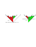
Figure 13: A charged Maya diagram $\mathsf{m}$ and the associated partition $Y\left(\mathsf{m}\right)$ for positive and negative charges $Q\left(\mathsf{m}\right)$. Given the positions $\mathsf{p}\left(\mathsf{m}\right)=\left(p_{1},\ldots,p_{r}\right)$ and $\mathsf{q}\left(\mathsf{m}\right)=\left(-q_{1},\ldots,-q_{s}\right)$ of particles and holes, the red and green areas represent the sums $\sum p_{k}$ and $\sum q_{k}$. We clearly have $\sum p_{k}+\sum q_{k}=\frac{{Q\left(\mathsf{m}\right)}^{2}}{2}+|Y\left(\mathsf{m}\right)|$ in both cases.

$\square$

In the Appendix, we show that the formula (4.24) can be rewritten in terms of Nekrasov functions. In the Painlev VI case ($n=4$), this transforms Theorem 4.6 into Theorem B of the Introduction.

4.2 Hypergeometric kernel

Recall that the matrices $\Theta_{0},\ldots,\Theta_{n-1}$ are by convention diagonal with eigenvalues distinct modulo non-zero integers. However, all of the results of Section 2 remain valid if the diagonal parts corresponding to the degenerate eigenvalues are replaced by appropriate Jordan blocks.

In this subsection we will consider in more detail a specific example of this type by revisiting the $4$-point tau function. We will thus follow the notational conventions of Subsection 2.5. Fix $n=4$, $N=2$ and assume furthermore that the monodromy representation $\rho^{[L]}:\pi_{1}\left(\mathbb{P}^{1}\backslash\left\{0,t,\infty\right\}\right)\to\mathrm{GL}\left(2,\mathbb{C}\right)$ associated to the internal trinion $\mathcal{T}^{[L]}$ is reducible, whereas its counterpart $\rho^{[R]}:\pi_{1}\left(\mathbb{P}^{1}\backslash\left\{0,1,\infty\right\}\right)\to\mathrm{GL}\left(2,\mathbb{C}\right)$ for the external trinion $\mathcal{T}^{[R]}$ remains generic. For instance, one may set

$$\begin{gathered}\Theta_{0}=\mathfrak{S}=\left(\begin{array}[]{cc}0&0\\ 0&-2\sigma\end{array}\right),\qquad\Theta_{t}=\left(\begin{array}[]{cc}0&0\\ 1&0\end{array}\right),\end{gathered}$$

so that the monodromy matrices $M_{0}$, $M_{t}$ can be assumed to have the lower triangular form

$$M_{0}=\left(\begin{array}[]{cc}1&0\\ -2\pi i\kappa e^{-2\pi i\sigma}&e^{-4\pi i\sigma}\end{array}\right),\qquad M_{t}=\left(\begin{array}[]{cc}1&0\\ 2\pi i\kappa e^{2\pi i\sigma}&1\end{array}\right),\qquad M_{0}M_{t}=e^{2\pi i\mathfrak{S}}.$$ (4.25)

The solution $\Psi^{[L]}\left(z\right)$ of the appropriate internal $3$-point RHP may be constructed from the fundamental solution of a Fuchsian system

$$\partial_{z}\Phi^{[L]}=\Phi^{[L]}\left(\begin{array}[]{cc}0&0\\ \displaystyle\frac{\varrho t}{z\left(z-t\right)}&\displaystyle-\frac{2\sigma}{z}\end{array}\right),$$ (4.26)

with a suitably chosen value of the parameter $\varrho$. Taking into account the diagonal monodromy around $\infty$, such a solution $\Phi^{[L]}\left(z\right)$ on $\mathbb{C}\backslash\mathbb{R}_{\geq 0}$ can be written as

$$\Phi^{[L]}\left(z\right)= \,\left(\begin{array}[]{cc}1&0\\ {\displaystyle\frac{\varrho t\left(-z\right)^{-2\sigma-1}}{1+2\sigma}}\,l_{2\sigma}\left(\frac{t}{z}\right)&\left(-z\right)^{-2\sigma}\end{array}\right)=\tilde{C}_{0}\left(\begin{array}[]{cc}1&0\\ {\displaystyle\frac{\varrho\left(-z\right)^{-2\sigma}}{2\sigma}}\,l_{-1-2\sigma}\left(\frac{z}{t}\right)&\left(-z\right)^{-2\sigma}\end{array}\right),$$ (4.31)

where $l_{a}\left(z\right):={}_{2}F_{1}\biggl{[}\begin{array}[]{c}1+a,1\vspace{-0.1cm}\\ 2+a\end{array};z\biggr{]}$, and the modified connection matrix $\tilde{C}_{0}$ is lower-triangular:

$$\tilde{C}_{0}=\left(\begin{array}[]{cc}1&0\\ \displaystyle-\frac{\pi\varrho t^{-2\sigma}}{\sin 2\pi\sigma}&1\end{array}\right).$$

The monodromy matrix around $0$ is clearly equal to $M_{0}=\tilde{C}_{0}e^{2\pi i\Theta_{0}}{\tilde{C}_{0}}^{-1}$. This allows to relate the monodromy parameter $\kappa$ to the coefficient $\rho$ of the Fuchsian system (4.26) as

$$\kappa=\varrho t^{-2\sigma}.$$ (4.32)

The $3$-point RHP solution $\Psi^{[L]}\left(z\right)$ inside the annulus $\mathcal{A}$ is thus explicitly given by

$$\Psi^{[L]}\left(z\right)\Bigl{|}_{\mathcal{A}}=\left(\begin{array}[]{cc}1&0\\ 0&\left(-z\right)^{2\sigma}\end{array}\right)\Phi^{[L]}\left(z\right)=\left(\begin{array}[]{cc}1&0\\ {\displaystyle-\frac{\varrho t}{\left(2\sigma+1\right)z}}\,l_{2\sigma}\left(\frac{t}{z}\right)&1\end{array}\right).$$ (4.33)

This formula leads to substantial simplifications in the Fredholm determinant representation (2.39) of the tau function $\tau_{\mathrm{JMU}}\left(t\right)$. It follows from from the structure of (4.33) and (2.40b) that

$$\mathsf{d}_{-+}\left(z,z^{\prime}\right)=\frac{\varrho}{1+2\sigma}\frac{\frac{t}{z}l_{2\sigma}\left(\frac{t}{z}\right)-\frac{t}{z^{\prime}}l_{2\sigma}\left(\frac{t}{z^{\prime}}\right)}{z-z^{\prime}}$$ (4.34)

is the only non-zero element of the $2\times 2$ matrix integral kernel $\mathsf{d}\left(z,z^{\prime}\right)$ (note that the lower indices here are color and should not be confused with half-integer Fourier modes). This in turn implies that the only entry of $\mathsf{a}\left(z,z^{\prime}\right)$ contributing to the determinant is

$$\mathsf{a}_{+-}\left(z,z^{\prime}\right)=\frac{1}{\operatorname{det}\Psi^{[R]}\left(z^{\prime}\right)}\frac{\Psi^{[R]}_{+-}\left(z\right)\Psi^{[R]}_{++}\left(z^{\prime}\right)-\Psi^{[R]}_{++}\left(z\right)\Psi^{[R]}_{+-}\left(z^{\prime}\right)}{z-z^{\prime}}.$$ (4.35)

Therefore, (2.39) reduces to

$$\tau_{\mathrm{JMU}}\left(t\right)=\operatorname{det}\left(\mathbb{1}-\mathsf{a}_{+-}\mathsf{d}_{-+}\right).$$ (4.36)

The action of the operators $\mathsf{a}_{+-}$, $\mathsf{d}_{-+}$ involves integration along a circle $\mathcal{C}\subset\mathcal{A}$. The kernel $\mathsf{a}_{+-}\left(z,z^{\prime}\right)$ extends to a function holomorphic in both arguments inside $\mathcal{C}$. Therefore in the computation of contributions of different exterior powers to the determinant one may try to shrink all integration contours to the branch cut $\mathcal{B}:=[0,t]\subset\mathbb{R}$. The latter comes from two branch points $0,t$ of $\mathsf{d}_{-+}\left(z,z^{\prime}\right)$ defined by (4.34).

Lemma 4.7.

Let $\left|\Re\sigma\right|<\frac{1}{2}$. For $m\in\mathbb{Z}_{\geq 0}$, denote $X_{m}=\operatorname{Tr}\left(\mathsf{a}_{+-}\mathsf{d}_{-+}\right)^{m}$. We have

$$X_{m}=\operatorname{Tr}K_{F}^{m},$$

where $K_{F}$ denotes an integral operator on $L^{2}\left(\mathcal{B}\right)$ with the kernel

$$K_{F}\left(z,z^{\prime}\right)=-\kappa\left(zz^{\prime}\right)^{\sigma}\mathsf{a}_{+-}\left(z,z^{\prime}\right).$$ (4.37)

Proof. Let us denote by $\mathcal{B}_{\text{up}}$ and $\mathcal{B}_{\text{down}}$ the upper and lower edge of the branch cut $\mathcal{B}$. After shrinking of the integration contours in the multiple integral $I_{k}$ to $\mathcal{B}$, the operators $\mathsf{a}_{+-}$, $\mathsf{d}_{-+}$ should be interpreted as acting on $\mathcal{W}=L^{2}\left(\mathcal{B}_{\text{up}}\right)\oplus L^{2}\left(\mathcal{B}_{\text{down}}\right)$ instead of $L^{2}\left(\mathcal{C}\right)$. Here $L^{2}\left(\mathcal{B}_{\text{up,down}}\right)$ arise as appropriate completions of spaces of boundary values of functions holomorphic inside $D_{\mathcal{C}}\backslash\mathcal{B}$, where $D_{\mathcal{C}}$ denotes the disk bounded by $\mathcal{C}$. The space $\mathcal{W}$ can be decomposed as $\mathcal{W}=\mathcal{W}_{+}\oplus\mathcal{W}_{-}$, where the elements of $\mathcal{W}_{+}$ are continuous across the branch cut, whereas the elements of $\mathcal{W}_{-}$ have opposite signs on its two sides:

$$\mathcal{W}_{\pm}=\left\{f\in\mathcal{W}\,:\,f\left(z+i0\right)=\pm f\left(z-i0\right),z\in\mathcal{B}\right\}.$$

We will denote by $\operatorname{pr}_{\pm}$ the projections on $\mathcal{W}_{\pm}$ along $\mathcal{W}_{\mp}$.

Since $\mathsf{a}_{+-}\left(z,z^{\prime}\right)$ is holomorphic in $z,z^{\prime}$ inside $\mathcal{C}$, it follows that $\operatorname{im}\mathsf{a}_{+-}\subseteq\mathcal{W}_{+}\subseteq\operatorname{ker}\mathsf{a}_{+-}$. Therefore $X_{k}$ remains unchanged if $\mathsf{a}_{+-}$ is replaced by $\operatorname{pr}_{+}\circ\,\mathsf{a}_{+-}\circ\operatorname{pr}_{-}$. This is in turn equivalent to replacing $\mathsf{d}_{-+}$ by $\operatorname{pr}_{-}\circ\,\mathsf{d}_{-+}\circ\operatorname{pr}_{+}$. Given $f=g\oplus g\in\mathcal{W}_{+}$ with $g\in L^{2}\left(\mathcal{B}\right)$, the action of $\mathsf{d}_{-+}$ on $f$ is given by

$$\left(\mathsf{d}_{-+}f\right)\left(z\right)= \,\frac{1}{2\pi i}\int_{0}^{t}\left[\mathsf{d}_{-+}\left(z,z^{\prime}-i0\right)-\mathsf{d}_{-+}\left(z,z^{\prime}+i0\right)\right]g\left(z^{\prime}\right)dz^{\prime}=$$

$$= \,\frac{\varrho t}{2\pi i\left(1+2\sigma\right)}\int_{0}^{t}\frac{l_{2\sigma}\left(\frac{t}{z^{\prime}+i0}\right)-l_{2\sigma}\left(\frac{t}{z^{\prime}-i0}\right)}{z^{\prime}\left(z-z^{\prime}\right)}\,g\left(z^{\prime}\right)dz^{\prime}.$$

An important consequence of the lower triangular monodromy is that the jump of $l_{2\sigma}\left(\frac{t}{z^{\prime}}\right)$ on $\mathcal{B}$ yields an elementary function, cf (4.31):

$$l_{2\sigma}\left(\frac{t}{z^{\prime}+i0}\right)-l_{2\sigma}\left(\frac{t}{z^{\prime}-i0}\right)=-2\pi i\left(2\sigma+1\right)\left(\frac{z^{\prime}}{t}\right)^{2\sigma+1}.$$

Substituting this jump back into the previous formula and using (4.32), one obtains

$$\left(\mathsf{d}_{-+}f\right)\left(z\right)=\kappa\int_{0}^{t}\frac{z^{\prime 2\sigma}g\left(z^{\prime}\right)dz^{\prime}}{z^{\prime}-z},\qquad\qquad z\in D_{\mathcal{C}}\backslash\mathcal{B}.$$

Next we have to compute the projection $\operatorname{pr}_{-}$ of this expression onto $\mathcal{W}_{-}$. Write $\operatorname{pr}_{-}\circ\,\mathsf{d}_{-+}f=h\oplus\left(-h\right)$, with ${h\in L^{2}\left(\mathcal{B}\right)}$. Then

$$h\left(z\right)=\frac{1}{2}\left[\left(\mathsf{d}_{-+}f\right)\left(z+i0\right)-\left(\mathsf{d}_{-+}f\right)\left(z-i0\right)\right]=\pi i\kappa z^{2\sigma}g\left(z\right),\qquad z\in\mathcal{B}.$$

Finally, write $\mathsf{a}_{+-}\circ\operatorname{pr}_{-}\circ\,\mathsf{d}_{-+}f$ as $\tilde{g}\oplus\tilde{g}\in\mathcal{W}_{+}$. It follows from the previous expression for $h\left(z\right)$ that

$$\tilde{g}\left(z\right)=-\kappa\int_{0}^{t}\mathsf{a}_{+-}\left(z,z^{\prime}\right){z^{\prime}}^{2\sigma}g\left(z^{\prime}\right)dz^{\prime},\qquad\qquad z\in\mathcal{B}.$$

The minus sign in front of the integral is related to orientation of the contour $\mathcal{C}$ in the definition of $\mathsf{a}$. We have thereby computed the action of $\mathsf{a}_{+-}\circ\operatorname{pr}_{-}\circ\,\mathsf{d}_{-+}$ on $\mathcal{W}_{+}$. Raising this operator to an arbitrary power $k\in\mathbb{Z}_{\geq 0}$ and symmetrizing the factors ${z^{\prime}}^{2\sigma}$ under the trace immediately yields the statement of the lemma. $\square$

Theorem 4.8.

Given complex parameters $\theta_{1},\theta_{\infty},\sigma$ satisfying previous genericity assumptions, let

$$\varphi\left(x\right):= \,x^{\sigma}\left(1-x\right)^{\theta_{1}}{}_{2}F_{1}\biggl{[}\begin{array}[]{c}\sigma+\theta_{1}+\theta_{\infty},\sigma+\theta_{1}-\theta_{\infty}\\ 2\sigma\end{array};x\biggr{]},$$ (4.38c)

$$\psi\left(x\right):= \,x^{1+\sigma}\left(1-x\right)^{\theta_{1}}{}_{2}F_{1}\biggl{[}\begin{array}[]{c}1+\sigma+\theta_{1}+\theta_{\infty},1+\sigma+\theta_{1}-\theta_{\infty}\\ 2+2\sigma\end{array};x\biggr{]}.$$ (4.38f)

Define the continuous ${}_{2}F_{1}$ kernel by

$$\tilde{K}_{F}\left(x,y\right):=\frac{\psi\left(x\right)\varphi\left(y\right)-\varphi\left(x\right)\psi\left(y\right)}{x-y},$$ (4.39)

and consider Fredholm determinant

$$D\left(t\right):=\operatorname{det}\left(\mathbf{1}-\lambda\tilde{K}_{F}\bigl{|}_{(0,t)}\bigr{.}\right),\qquad\lambda\in\mathbb{C}.$$ (4.40)

Then $D\left(t\right)$ is a tau function of the Painlevé VI equation with parameters $\vec{\theta}=\left(\theta_{0}=\sigma,\theta_{t}=0,\theta_{1},\theta_{\infty}\right)$. The conjugacy class of monodromy representation for the associated $4$-point Fuchsian system is generated by the matrices (4.25) and

$$M_{1}= \,\frac{e^{-2\pi i\theta_{1}}}{i\sin 2\pi\sigma}\left(\begin{array}[]{cc}\cos 2\pi\theta_{\infty}-e^{-2\pi i\sigma}\cos 2\pi\theta_{1}&s^{-1}e^{-2\pi i\sigma}\left[\cos 2\pi\theta_{\infty}-\cos 2\pi\left(\theta_{1}-\sigma\right)\right]\\ se^{2\pi i\sigma}\left[\cos 2\pi\left(\theta_{1}+\sigma\right)-\cos 2\pi\theta_{\infty}\right]&e^{2\pi i\sigma}\cos 2\pi\theta_{1}-\cos 2\pi\theta_{\infty}\end{array}\right),$$ (4.41c)

$$M_{\infty}= \,\frac{e^{-2\pi i\theta_{\infty}}}{i\sin 2\pi\sigma}\left(\begin{array}[]{cc}\cos 2\pi\theta_{1}-e^{-2\pi i\sigma}\cos 2\pi\theta_{\infty}&s^{-1}\left[\cos 2\pi\left(\theta_{1}-\sigma\right)-\cos 2\pi\theta_{\infty}\right]\\ s\left[\cos 2\pi\theta_{\infty}-\cos 2\pi\left(\theta_{1}+\sigma\right)\right]&e^{2\pi i\sigma}\cos 2\pi\theta_{\infty}-\cos 2\pi\theta_{1}\end{array}\right)=M_{1}^{-1}e^{-2\pi i\mathfrak{S}}.$$ (4.41f)

where

$$\lambda=\kappa\frac{\left(\theta_{1}+\sigma\right)^{2}-\theta_{\infty}^{2}}{2\sigma\left(2\sigma+1\right)},$$ (4.42)

$$s=-\frac{\Gamma\left(1-2\sigma\right)\Gamma\left(\theta_{1}+\sigma+\theta_{\infty}\right)\Gamma\left(\theta_{1}+\sigma-\theta_{\infty}\right)}{\Gamma\left(1+2\sigma\right)\Gamma\left(\theta_{1}-\sigma+\theta_{\infty}\right)\Gamma\left(\theta_{1}-\sigma-\theta_{\infty}\right)}.$$ (4.43)

Proof. To prove that $D\left(t\right)$ is a Painlevé VI tau function with $\lambda$ and $\kappa$ related by (4.42), it suffices to combine the determinant representation (4.36) with Lemma 4.7, and substitute into the formula (4.35) for $\mathsf{a}_{+-}\left(z,z^{\prime}\right)$ explicit hypergeometric expressions (4.8).

The formula (4.41f) follows from $M_{\infty}=C_{\infty}e^{2\pi i\Theta_{\infty}}C_{\infty}^{-1}$, where $C_{\infty}$ is obtained from the connection matrix (4.17) by replacements $\left(\theta_{k},\sigma_{k-1},\sigma_{k}\right)\to\left(\theta_{1},\sigma,-\theta_{\infty}\right)$. The expression (4.41c) for $M_{1}$ is then most easily deduced from the diagonal form of the product $M_{1}M_{\infty}=e^{-2\pi i\mathfrak{S}}$. $\square$

Remark 4.9.

The ${}_{2}F_{1}$ kernel is related to the so-called $ZW$-measures [BO1] arising in the representation theory of the infinite-dimensional unitary group $U\left(\infty\right)$. It produces various other classical integrable kernels (such as sine and Whittaker) as limiting cases. The first part of Theorem 4.8, namely the Painlevé VI equation for $D\left(t\right)$, was proved by Borodin and Deift in [BD]. Monodromy data for the associated Fuchsian system have been identified in [Lis]. To facilitate the comparison, let us note that indroducing instead of $\lambda$ and $\kappa$ a new parameter $\bar{\sigma}$ defined by

$$\lambda=\frac{\sin\pi\left(\bar{\sigma}-\theta_{1}\right)\sin\pi\left(\bar{\sigma}+\theta_{1}\right)}{\pi^{2}}\frac{\prod_{\epsilon,\epsilon^{\prime}=\pm}\Gamma\left(1+\sigma+\epsilon\theta_{1}+\epsilon^{\prime}\theta_{\infty}\right)}{\Gamma\left(1+2\sigma\right)\Gamma\left(2+2\sigma\right)},$$

we have in particular that $\operatorname{Tr}M_{\infty}M_{0}=2e^{-2\pi i\left(\sigma+\theta_{\infty}\right)}\cos 2\pi\bar{\sigma}$ and $\operatorname{Tr}M_{t}M_{1}=2e^{2\pi i\left(\sigma+\theta_{\infty}\right)}\cos 2\pi\bar{\sigma}$. The relation between parameters $z,z^{\prime},w,w^{\prime}$ of [BD] and ours is

$$\left(z,z^{\prime},w,w^{\prime}\right)_{\text{\cite[cite]{[\@@bibref{}{BorodinDeift}{}{}]}}}=\left(\bar{\sigma}+\theta_{1},\bar{\sigma}-\theta_{1},\sigma-\bar{\sigma}+\theta_{\infty},\sigma-\bar{\sigma}-\theta_{\infty}\right).$$

Appendix A Relation to Nekrasov functions

Here we demonstrate that the formula (4.24) can be rewritten in terms of Nekrasov functions. This rewrite is conceptually important for identification of isomonodromic tau functions with dual partition functions of quiver gauge theories [NO]. It is also useful from a computational point of view: naively, the formula (4.24) may produce poles in the tau function expansion coefficients when $\theta_{k}\pm\sigma_{k}\pm^{\prime}\sigma_{k-1}\in\mathbb{Z}$. Our calculation shows that these poles actually cancel.

The statement we are going to prove is the relation

$$\begin{gathered}Z^{\vec{Y}^{\prime},m^{\prime}}_{\vec{Y},m}\left(\mathcal{T}\right)=(-1)^{{\rm lsgn}\left(\vec{Y}^{\prime},m^{\prime}\right)+{\rm lsgn}\left(\vec{Y},m\right)}\hat{Z}^{\vec{Y}^{\prime},\vec{Q}^{\prime}}_{\vec{Y},\vec{Q}}\left(\mathcal{T}\right),\end{gathered}$$ (A.1)

where

$$\begin{aligned} \hat{Z}^{\vec{Y}^{\prime},\vec{Q}^{\prime}}_{\vec{Y},\vec{Q}}(\mathcal{T})=&\,\frac{\prod_{\alpha,\beta}^{N}C\left(\left.\sigma^{\prime}_{\alpha}-\sigma_{\beta}\right|Q^{\prime}_{\alpha},Q_{\beta}\right)}{\prod_{\alpha<\beta}^{N}C\bigl{(}\bigl{.}\sigma^{\prime}_{\alpha}-\sigma^{\prime}{}_{\beta}\bigr{|}Q^{\prime}_{\alpha},Q^{\prime}_{\beta}\bigr{)}\,C\bigl{(}\sigma_{\alpha}-\sigma_{\beta}|Q_{\alpha},Q_{\beta}\bigr{)}}\frac{\left(-1\right)^{N|\vec{Y}|+\frac{N}{2}|\vec{Q}|^{2}}e^{i\delta\vec{\eta}^{\prime}\cdot\vec{Q}^{\prime}+i\delta\vec{\eta}\cdot\vec{Q}}}{\prod_{\alpha}^{N}\left|Z_{\,\mathsf{bif}}\left(0\bigl{|}\bigr{.}Y_{\alpha},Y_{\alpha}\right)\right|^{\frac{1}{2}}\left|Z_{\,\mathsf{bif}}\left(0\bigl{|}\bigr{.}Y^{\prime}_{\alpha},Y^{\prime}_{\alpha}\right)\right|^{\frac{1}{2}}}\times\\ \times&\,\frac{\prod_{\alpha,\beta}^{N}Z_{\,\mathsf{bif}}\left(\left.\sigma^{\prime}_{\alpha}+Q^{\prime}_{\alpha}-\sigma_{\beta}-Q_{\beta}\right|Y^{\prime}_{\alpha},Y_{\beta}\right)}{\prod_{\alpha<\beta}^{N}Z_{\,\mathsf{bif}}\bigl{(}\bigl{.}\sigma^{\prime}_{\alpha}+Q^{\prime}_{\alpha}-\sigma^{\prime}_{\beta}-Q^{\prime}_{\beta}\bigr{|}Y^{\prime}_{\alpha},Y^{\prime}_{\beta}\bigr{)}\,Z_{\,\mathsf{bif}}\left(\left.\sigma_{\alpha}+Q_{\alpha}-\sigma_{\beta}-Q_{\beta}\right|Y_{\alpha},Y_{\beta}\right)}.\end{aligned}$$ (A.2)

The notation used in these formulas means the following:

• $\vec{Q}=\left(m,-m\right)$, $\vec{Q}^{\prime}=\left(m^{\prime},-m^{\prime}\right)$, though the right side of (A.2) is defined even without this specialization.

• $Y^{\prime}$ and $Y$ are identified, respectively, with $Y_{k-1}$ and $Y_{k}$ in (4.24). Similar conventions will be used for all other quantities. We denote, however, $\sigma^{\prime}_{\pm}=\pm\sigma_{k-1}$ and $\sigma_{\pm}=-\theta_{k}\pm\sigma_{k}$; $\mathcal{T}$ stands for $\mathcal{T}^{[k]}$.

• ${\rm lsgn}\left(\vec{Y},m\right)\in\mathbb{Z}/2\mathbb{Z}$ means the “logarithmic $\rm sign$”,

  $$\begin{gathered}{\rm lsgn}\left(\vec{Y},m\right):=|\mathsf{q}_{+}|\cdot|\mathsf{p}_{+}|+\sum\limits_{i}\left(q_{+,i}+\frac{1}{2}\right)+\sum\limits_{i}\left(p_{-,i}+\frac{1}{2}\right).\end{gathered}$$ (A.3)

  Here, for example, $|\mathsf{p}_{+}|$ denotes the number of coordinates $p_{+,i}$ of particles in the Maya diagram corresponding to the charged partition $\left(Y_{+},m\right)$. The logarithmic signs cancel in the product $\prod_{k=1}^{n-2}Z^{\vec{Y}_{k-1},m_{k-1}}_{\;\vec{Y}_{k},m_{k}}$ which appears in the representation (4.23) for the Garnier tau function.

• $\delta\vec{\eta}$ and $\delta\vec{\eta}^{\prime}$ are some explicit functions which are computed below. They just shift Fourier transformation parameters and their relevant combinations are explicitly given by

  $$\begin{aligned} e^{i\delta\eta^{\prime}_{+}-i\delta\eta^{\prime}_{-}}&=\frac{1}{2\sigma_{k-1}}\frac{\left(\theta_{k}+\sigma_{k-1}\right)^{2}-\sigma_{k}^{2}}{\left(\theta_{k}-\sigma_{k-1}\right)^{2}-\sigma_{k}^{2}},\\ e^{i\delta\eta_{+}-i\delta\eta_{-}}&=\;\;\;\frac{-1}{2\,\sigma_{k}}\;\,\frac{\left(\theta_{k}+\sigma_{k}\right)^{2}-\sigma_{k-1}^{2}}{\left(\theta_{k}-\sigma_{k}\right)^{2}-\sigma_{k-1}^{2}}.\end{aligned}$$ (A.4)

• $Z_{\,\mathsf{bif}}\left(\nu|Y^{\prime},Y\right)$ is the Nekrasov bifundamental contribution

  $$Z_{\,\mathsf{bif}}\left(\nu|Y^{\prime},Y\right):=\prod_{\square\in Y^{\prime}}\bigl{(}\nu+1+a_{Y^{\prime}}\left(\square\right)+l_{Y}\left(\square\right)\bigr{)}\prod_{\square\in Y}\bigl{(}\nu-1-a_{Y}\left(\square\right)-l_{Y^{\prime}}\left(\square\right)\bigr{)}.$$ (A.5)

  In particular, we have $\left|Z_{\,\mathsf{bif}}\left(0|Y,Y\right)\right|^{\frac{1}{2}}=\prod_{\square\in Y}h_{Y}\left(\square\right)$.

• The three-point function $C\left(\nu|Q^{\prime},Q\right)$ is defined by

  $$\begin{gathered}C\left(\nu|Q^{\prime},Q\right)\equiv C\left(\nu|Q^{\prime}-Q\right)=\frac{G\left(1+\nu+Q^{\prime}-Q\right)}{G\left(1+\nu\right)\Gamma\left(1+\nu\right)^{Q^{\prime}-Q}},\end{gathered}$$ (A.6)

  where $G\left(x\right)$ is the Barnes $G$-function. The only property of this function essential for our purposes is the recurrence relation $G\left(x+1\right)=\Gamma\left(x\right)G\left(x\right)$.

• Using the formula (4.24), we assume a concrete ordering: $p_{+}^{\prime},p_{-}^{\prime},q_{+},q_{-}$, $p_{1}>p_{2}>\ldots$, and in (A.2) we suppose that $+<-$.

An important feature of the product (A.2) is that the combinatorial part in the 2nd line depends only on combinations such as $\sigma_{\alpha}+Q_{\alpha}$, $\sigma^{\prime}_{\alpha}+Q^{\prime}_{\alpha}$. This is most crucial for the Fourier transform structure of the full aswer for the tau function $\tau_{\mathrm{Garnier}}\left(a\right)$.

Let us now present the plan of the proof, which will be divided into several self-contained parts. Most computations will be done up to an overall sign, and sometimes we will omit to indicate this. In the end we will consider the limit $\theta_{k}\to+\infty$, $\sigma_{k},\sigma_{k-1}\ll\theta_{k}$, $\sigma_{k},\sigma_{k-1}\to+\infty$ to recover the correct sign.

1. First we will rewrite the formula (4.24) as

   $$Z^{\vec{Y}^{\prime},m^{\prime}}_{\vec{Y},m}\left(\mathcal{T}\right)=\pm e^{i\delta_{1}\vec{\eta}^{\prime}\cdot\vec{Q}^{\prime}+i\delta_{1}\vec{\eta}\cdot\vec{Q}}\hat{\hat{Z}}^{\vec{Y}^{\prime},\vec{Q}^{\prime}}_{\vec{Y},\vec{Q}}\left(\mathcal{T}\right),$$

   where $\hat{\hat{Z}}^{\vec{Y}^{\prime},\vec{Q}^{\prime}}_{\vec{Y},\vec{Q}}\left(\mathcal{T}\right)$ is expressed in terms of yet another function $\tilde{Z}_{\,\mathsf{bif}}\left(\nu\bigl{|}Q^{\prime},Y^{\prime};Q,Y\right)$,

   $$\begin{aligned} \hat{\hat{Z}}^{\vec{Y}^{\prime},\vec{Q}^{\prime}}_{\vec{Y},\vec{Q}}\left(\mathcal{T}\right)=&\;\prod_{\alpha}^{N}\,\bigl{|}\tilde{Z}_{\mathsf{bif}}\left(0\bigl{|}Q_{\alpha},Y_{\alpha},Q_{\alpha},Y_{\alpha}\right)\bigr{|}^{-\frac{1}{2}}\bigl{|}\tilde{Z}_{\mathsf{bif}}\left(0\bigl{|}Q^{\prime}_{\alpha},Y^{\prime}_{\alpha},Q^{\prime}_{\alpha},Y^{\prime}_{\alpha}\right)\bigr{|}^{-\frac{1}{2}}\;\times\\ \times&\,\frac{\prod_{\alpha,\beta}^{N}\tilde{Z}_{\mathsf{bif}}\left(\sigma^{\prime}_{\alpha}-\sigma_{\beta}\bigl{|}Q^{\prime}_{\alpha},Y^{\prime}_{\alpha};Q_{\beta},Y_{\beta}\right)}{\prod_{\alpha<\beta}^{N}\tilde{Z}_{\,\mathsf{bif}}\bigl{(}\sigma^{\prime}_{\alpha}-\sigma^{\prime}_{\beta}\bigl{|}Q^{\prime}_{\alpha},Y^{\prime}_{\alpha};Q^{\prime}_{\beta},Y^{\prime}_{\beta}\bigr{)}\tilde{Z}_{\,\mathsf{bif}}\left(\sigma_{\alpha}-\sigma_{\beta}\bigl{|}Q_{\alpha},Y_{\alpha};Q_{\beta},Y_{\beta}\right)},\end{aligned}$$ (A.7)

   which is defined as

   $$\begin{aligned} \tilde{Z}_{\,\mathsf{bif}}\left(\nu\bigl{|}Q^{\prime},Y^{\prime};Q,Y\right)=&\,\prod_{i}\left(-\nu\right)_{q_{i}^{\prime}+\frac{1}{2}}\prod_{i}\left(\nu+1\right)_{q_{i}-\frac{1}{2}}\prod_{i}\left(-\nu\right)_{p_{i}+\frac{1}{2}}\prod_{i}\left(\nu+1\right)_{p_{i}^{\prime}-\frac{1}{2}}\times\\ \times&\,\frac{\prod_{i,j}\left(\nu-q_{i}^{\prime}-p_{j}\right)\prod_{i,j}\left(\nu+p_{i}^{\prime}+q_{j}\right)}{\prod_{i,j}\left(\nu-q_{i}^{\prime}+q_{j}\right)\prod_{i,j}\left(\nu+p_{i}^{\prime}-p_{j}\right)}.\end{aligned}$$ (A.8)

2. At the second step, we prove that $\tilde{Z}_{\,\mathsf{bif}}\left(\nu\bigl{|}0,Y^{\prime};0,Y\right)\equiv\tilde{Z}_{\,\mathsf{bif}}\left(\nu\bigl{|}Y^{\prime},Y\right)=\pm Z_{\,\mathsf{bif}}\left(\nu\bigl{|}Y^{\prime},Y\right)$.

3. Next it will be shown that

   $$\tilde{Z}_{\,\mathsf{bif}}\left(\nu\bigl{|}Q^{\prime},Y^{\prime};Q,Y\right)=C\left(\nu\bigl{|}Q^{\prime},Q\right)Z_{\,\mathsf{bif}}\left(\nu+Q^{\prime}-Q\bigl{|}Y^{\prime},Y\right).$$ (A.9)

4. Finally, we check the overall sign and compute extra contribution to $\vec{\eta}$ to absorb it.

A realization of this plan is presented below.

Step 1

It is useful to decompose the product (4.24) into two different parts: a “diagonal” one, containing the products of functions of one particle/hole coordinate, and a “non-diagonal” part containing the products of pairwise sums/differences. Careful comparison of the formulas (4.24) and (A.7) shows that their non-diagonal parts actually coincide. Further analysis of (A.7) shows that its diagonal part is given by

$$\prod_{\left(p^{\prime},\epsilon\right)\in I^{\prime}}\psi_{p^{\prime},\epsilon}\prod_{\left(-q^{\prime},\epsilon\right)\in J^{\prime}}\bar{\psi}_{q^{\prime},\epsilon}\prod_{\left(-q,\epsilon\right)\in J}\varphi_{q,\epsilon}\prod_{\left(p,\epsilon\right)\in I}\bar{\varphi}_{p,\epsilon}.$$

with

$$\begin{aligned} \psi_{p^{\prime},\epsilon}&=\frac{\left(1+\epsilon\sigma_{k-1}+\theta_{k}-\sigma_{k}\right)_{p^{\prime}-\frac{1}{2}}\left(1+\epsilon\sigma_{k-1}+\theta_{k}+\sigma_{k}\right)_{p^{\prime}-\frac{1}{2}}}{\bigl{[}\epsilon=+:\left(1+2\sigma_{k-1}\right)_{p^{\prime}-\frac{1}{2}};\,\epsilon=-:\left(-2\sigma_{k-1}\right)_{p^{\prime}+\frac{1}{2}}\bigr{]}\left(p^{\prime}-\frac{1}{2}\right)!},\\ \bar{\psi}_{q^{\prime},\epsilon}&=\frac{\left(-\epsilon\sigma_{k-1}-\theta_{k}+\sigma_{k}\right)_{q^{\prime}+\frac{1}{2}}\left(-\epsilon\sigma_{k-1}-\theta_{k}-\sigma_{k}\right)_{q^{\prime}+\frac{1}{2}}}{\bigl{[}\epsilon=+:\left(-2\sigma_{k-1}\right)_{q^{\prime}+\frac{1}{2}};\,\epsilon=-:\left(1+2\sigma_{k-1}\right)_{q^{\prime}-\frac{1}{2}}\bigr{]}\left(q^{\prime}-\frac{1}{2}\right)!},\\ \varphi_{q,\epsilon}&=\frac{\left(\sigma_{k-1}+\theta_{k}-\epsilon\sigma_{k}+1\right)_{q-\frac{1}{2}}\left(-\sigma_{k-1}+\theta_{k}-\epsilon\sigma_{k}+1\right)_{q-\frac{1}{2}}}{\bigl{[}\epsilon=+:\left(-2\sigma_{k}\right)_{q+\frac{1}{2}};\,\epsilon=-:\left(1+2\sigma_{k}\right)_{q-\frac{1}{2}}\bigr{]}\left(q-\frac{1}{2}\right)!},\\ \bar{\varphi}_{p,\epsilon}&=\frac{\left(-\sigma_{k-1}-\theta_{k}+\epsilon\sigma_{k}\right)_{p+\frac{1}{2}}\left(\sigma_{k-1}-\theta_{k}+\epsilon\sigma_{k}\right)_{p+\frac{1}{2}}}{\bigl{[}\epsilon=+:\left(1+2\sigma_{k}\right)_{p-\frac{1}{2}};\,\epsilon=-:\left(-2\sigma_{k}\right)_{p+\frac{1}{2}}\bigr{]}\left(p-\frac{1}{2}\right)!}.\end{aligned}$$ (A.10)

The notation $[\epsilon=+:X;\epsilon=-:Y]$ means that we should substitute this construction by $X$ when $\epsilon=+$ and by $Y$ when $\epsilon=-$. Comparing these expressions with (4.24), we may compute the ratios of diagonal factors which appear in $Z^{\vec{Y}^{\prime},m^{\prime}}_{\;\vec{Y},m}\bigl{/}\hat{\hat{Z}}^{\vec{Y}^{\prime},\vec{Q}^{\prime}}_{\vec{Y},\vec{Q}}\bigr{.}$:

$$\begin{gathered}\begin{split}\delta\psi_{p^{\prime},\epsilon}&=\frac{\left(\epsilon\sigma_{k-1}+\theta_{k}-\sigma_{k}\right)\left(\epsilon\sigma_{k-1}+\theta_{k}+\sigma_{k}\right)}{[\epsilon=+:2\sigma_{k-1};\,\epsilon=-:1]},\\ \delta\bar{\psi}_{q^{\prime},\epsilon}&=\frac{\left(-\epsilon\sigma_{k-1}-\theta_{k}+\sigma_{k}\right)^{-1}\left(-\epsilon\sigma_{k-1}-\theta_{k}-\sigma_{k}\right)^{-1}}{[\epsilon=+:\left(-2\sigma_{k-1}\right)^{-1};\,\epsilon=-:1]},\\ \delta\varphi_{q,\epsilon}&=\frac{\left(\sigma_{k-1}+\theta_{k}-\epsilon\sigma_{k}\right)\left(-\sigma_{k-1}+\theta_{k}-\epsilon\sigma_{k}\right)}{[\epsilon=+:1;\,\epsilon=-:2\sigma_{k}]},\\ \delta\bar{\varphi}_{p,\epsilon}&=\frac{\left(-\sigma_{k-1}-\theta_{k}+\epsilon\sigma_{k}\right)^{-1}\left(\sigma_{k-1}-\theta_{k}+\epsilon\sigma_{k}\right)^{-1}}{[\epsilon=+:1;\,\epsilon=-:\left(-2\sigma_{k}\right)^{-1}]}.\end{split}\end{gathered}$$ (A.11)

Since $|\mathsf{p}_{\pm}|-|\mathsf{q}_{\pm}|=Q_{\pm}$, these formulas allow to determine the corrections $\delta_{1}\eta_{\pm}$:

$$\begin{aligned} e^{i\delta_{1}\eta^{\prime}_{+}}&=\frac{\left(\theta_{k}+\sigma_{k-1}\right)^{2}-\sigma_{k}^{2}}{2\sigma_{k-1}},\qquad e^{-i\delta_{1}\eta_{+}}=\,\left(\theta_{k}-\sigma_{k}\right)^{2}-\sigma_{k-1}^{2},\\ e^{i\delta_{1}\eta^{\prime}_{-}}&=\,\left(\theta_{k}-\sigma_{k-1}\right)^{2}-\sigma_{k}^{2},\qquad e^{-i\delta_{1}\eta_{-}}=\frac{\left(\theta_{k}+\sigma_{k}\right)^{2}-\sigma_{k-1}^{2}}{2\sigma_{k}}.\end{aligned}$$ (A.12)

One could notice that some minus signs should also be taken into account, so that

$$Z^{\vec{Y}^{\prime},m^{\prime}}_{\vec{Y},m}\left(\mathcal{T}\right)=\left(-1\right)^{|\mathsf{q}_{+}^{\prime}|+|\mathsf{p}_{-}|}e^{i\delta_{1}\vec{\eta}^{\prime}\cdot\vec{Q}^{\prime}+i\delta_{1}\vec{\eta}\cdot\vec{Q}}\hat{\hat{Z}}^{\vec{Y}^{\prime},\vec{Q}^{\prime}}_{\vec{Y},\vec{Q}}\left(\mathcal{T}\right).$$

This is however not essential, as these signs will be recovered at the last step. A more important thing to note is that in the reference limit described by $\theta_{k}\to+\infty$, $\sigma_{k},\sigma_{k-1}\ll\theta$, $\sigma_{k},\sigma_{k-1}\to+\infty$ one has

$${\rm sgn}\bigl{(}e^{i\delta_{1}\eta_{\pm}}\bigr{)}={\rm sgn}\bigl{(}e^{i\delta_{1}\eta^{\prime}_{\pm}}\bigr{)}=1.$$

Step 2

Let us now formulate and prove combinatorial

Theorem A.1.

$\tilde{Z}_{\,\mathsf{bif}}\left(\nu\bigl{|}0,Y^{\prime};0,Y\right)\equiv\tilde{Z}_{\,\mathsf{bif}}\left(\nu\bigl{|}Y^{\prime},Y\right)=\pm Z_{\,\mathsf{bif}}\left(\nu\bigl{|}Y^{\prime},Y\right)$.

This statement follows from the following two lemmas.

Lemma A.2.

Equality $Z_{\,\mathsf{bif}}=\pm\tilde{Z}_{\,\mathsf{bif}}$ holds for the diagrams $Y^{\prime},Y\in\mathbb{Y}$ iff it holds for $Y^{\prime},Y$ with added one column of admissible height $L$.

Proof. Let us denote the new value of $Z_{\,\mathsf{bif}}$ by $Z_{\,\mathsf{bif}}^{*}$ , then

$$\begin{gathered}Z_{\,\mathsf{bif}}^{*}=\frac{\left(1+\nu\right)_{L}\prod_{i}\left(L+p_{i}^{\prime}+\frac{1}{2}+\nu\right)}{\prod_{i}\left(L-q_{i}^{\prime}+\frac{1}{2}+\nu\right)}\frac{\left(1-\nu\right)_{L}\prod_{i}\left(L+p_{i}+\frac{1}{2}-\nu\right)}{\prod_{i}\left(L-q_{i}+\frac{1}{2}-\nu\right)}Z_{\,\mathsf{bif}}.\end{gathered}$$ (A.13)

The extra factor comes only from the product over $2L$ new boxes. To explain how its expression is obtained, we will use the conventions of Fig. 14.

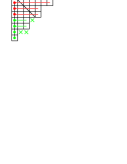
Figure 14: A Young diagram $Y^{\prime*}$ obtained from $Y^{\prime}=\left\{6,4,4,2,2\right\}$ by addition of a column of length $L=7$.

To compute the contribution from the red boxes it is enough just to multiply the corresponding shifted hook lengths, which yields $\prod_{i}\left(L+p_{i}^{\prime}+\frac{1}{2}+\nu\right)$. To compute the contribution from the green boxes one has to first write down the product of numbers from $\nu+L$ to $\nu+1$ (i.e. the Pochhammer symbol $\left(1+\nu\right)_{L}$ in the numerator), keeping in mind that each step down by one box decreases the leg-length of the box by at least one. Then one has to take into account that some jumps in this sequence are greater than one: this happens exactly when we meet some rows of the transposed diagram. We mark with the green crosses the boxes whose contributions should be cancelled from the initial product: they produce the denominator.

Next let us check what happens with $\tilde{Z}_{\,\mathsf{bif}}$. We have

$$\tilde{Z}_{\,\mathsf{bif}}^{*}\left(\nu|Y^{\prime},Y\right)=\prod_{i}\left(-\nu\right)_{q_{i}^{\prime*}+\frac{1}{2}}\prod_{i}\nu^{-1}\left(\nu\right)_{q_{i}^{*}+\frac{1}{2}}\prod_{i}\left(-\nu\right)_{p_{i}^{*}+\frac{1}{2}}\prod_{i}\nu^{-1}\left(\nu\right)_{p_{i}^{\prime*}+\frac{1}{2}}\frac{\prod_{i,j}\left(\nu-q_{i}^{\prime*}-p_{j}^{*}\right)\prod_{i,j}\left(\nu+p_{i}^{\prime*}+q_{j}^{*}\right)}{\prod_{i,j}\left(q_{i}^{\prime*}-q_{j}^{*}-\nu\right)\prod_{i,j}\left(p_{i}^{\prime*}-p_{j}^{*}+\nu\right)},$$

where

$$\left\{q_{i}^{*}\right\}=\left\{\left(L-1/2\right),\left(q_{1}-1\right),\ldots,\left(q_{d-1}-1\right),\widetilde{(q_{d}-1)}\right\},$$

$$\left\{p_{i}^{*}\right\}=\left\{\left(p_{1}+1\right),\ldots,\left(p_{d}+1\right),\widetilde{1/2}\right\},$$

$$\left\{q_{i}^{\prime*}\right\}=\bigl{\{}\left(L-1/2\right),\left(q^{\prime}_{1}-1\right),\ldots,\left(q^{\prime}_{d^{\prime}-1}-1\right),\widetilde{\widetilde{(q^{\prime}_{d^{\prime}}-1)}}\bigr{\}},$$

$$\left\{p_{i}^{\prime*}\right\}=\bigl{\{}\left(p^{\prime}_{1}+1\right),\ldots,\left(p^{\prime}_{d^{\prime}}+1\right),\widetilde{\widetilde{1/2}}\bigr{\}},$$

and $d,d^{\prime}$ denote the number of boxes on the main diagonals of $Y,Y^{\prime}$. The above notation means that one has either to simultaneously include or not to include the coordinates tilded in the same way. These numbers are included in the case when both of them are positive (it implies that $q_{d}\neq\frac{1}{2}$ or $q^{\prime}_{d^{\prime}}\neq\frac{1}{2}$). Fig. 15 below illustrates the difference between these two cases.

Figure 15: Possible mutual configurations of main diagonals of $Y$, $Y^{*}$; $q_{d}=\frac{1}{2}$ (left) and $q_{d}\neq\frac{1}{2}$ (right).

We may now consider one by one four possible options, namely: i) $q_{d}\neq\frac{1}{2}$, $q^{\prime}_{d^{\prime}}\neq\frac{1}{2}$; ii) $q_{d}=q^{\prime}_{d^{\prime}}=\frac{1}{2}$; iii) ${q_{d}\neq\frac{1}{2}}$, $q^{\prime}_{d^{\prime}}=\frac{1}{2}$; iv) $q_{d}=\frac{1}{2}$, $q^{\prime}_{d^{\prime}}\neq\frac{1}{2}$. For instance, for $q_{d}\neq\frac{1}{2}$, $q^{\prime}_{d^{\prime}}\neq\frac{1}{2}$ after massive cancellations one obtains

$$\begin{aligned} \frac{\tilde{Z}_{\,\mathsf{bif}}^{*}}{\tilde{Z}_{\,\mathsf{bif}}}=&\,\prod_{i=1}^{d^{\prime}}\frac{1}{-\nu+q_{i}^{\prime}-\frac{1}{2}}\left(-\nu\right)_{L}\prod_{i=1}^{d}\frac{1}{\nu+q_{i}-\frac{1}{2}}\nu^{-1}\left(\nu\right)_{L}\prod_{i=1}^{d}\left(-\nu+p_{i}+\frac{1}{2}\right)\left(-\nu\right)_{1}\prod_{i=1}^{d^{\prime}}\left(\nu+p_{i}^{\prime}+\frac{1}{2}\right)\times\\ \times&\,\frac{\prod_{i}\left(\nu-L-\frac{1}{2}-p_{i}\right)\prod_{i}\left(\nu-q_{i}^{\prime}+\frac{1}{2}\right)\prod_{i}\left(\nu-\frac{1}{2}+q_{i}\right)\prod_{i}\left(\nu+p_{i}^{\prime}+L+\frac{1}{2}\right)}{\prod_{i}\left(L+\frac{1}{2}-q_{i}-\nu\right)\prod_{i}\left(q_{i}^{\prime}-L-\frac{1}{2}-\nu\right)\prod_{i}\left(p_{i}^{\prime}+\frac{1}{2}+\nu\right)\prod_{i}\left(-\frac{1}{2}-p_{i}+\nu\right)}\frac{\left(\nu-L\right)\left(\nu+L\right)}{\nu^{2}}=\\ =&\ \left(1-\nu\right)_{L}\left(1+\nu\right)_{L}\frac{\prod_{i}(\nu-L-\frac{1}{2}-p_{i})\prod_{i}(\nu+p^{\prime}_{i}+L+\frac{1}{2})}{\prod_{i}(L+\frac{1}{2}-q_{i}-\nu)\prod_{i}(q_{i}^{\prime}-L-\frac{1}{2}-\nu)}=\frac{Z_{\,\mathsf{bif}}^{*}}{Z_{\,\mathsf{bif}}},\end{aligned}$$

where the first line of the first equality corresponds to the ratio of diagonal parts and the second to non-diagonal ones. The proof in the other three cases is analogous. $\square$

Corollary A.3.

$Z_{\,\mathsf{bif}}=\tilde{Z}_{\,\mathsf{bif}}$ for arbitrary $Y,Y^{\prime}\in\mathbb{Y}$ iff $Z_{\,\mathsf{bif}}=\pm Z_{\,\mathsf{bif}}^{*}$ for diagrams with $\left\{q_{i}\right\}=\left\{\frac{1}{2},\ldots,L-\frac{1}{2}\right\}$ (that is, for the diagrams containing a large square on the left).

Lemma A.4.

The equality $Z_{\,\mathsf{bif}}=\tilde{Z}_{\,\mathsf{bif}}$ holds for given diagrams $Y,Y^{\prime}\in\mathbb{Y}$ with a large square iff it holds for the diagrams with a large square and one deleted box.

Proof.

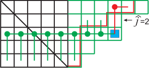
Figure 16: A pair of Young diagrams (red and green) with a large square (black) and added box (blue square).

Suppose that we have added one box to the $i$th row of $Y^{\prime}$. The only boxes whose contribution to $Z_{\,\mathsf{bif}}$ depends on the added box lie on its left in the diagram $Y^{\prime}$ and above it in the diagram $Y$, see Fig. 16. The contribution from the boxes on the left (green circles) was initially given by

$$Z_{\,\mathsf{bif}}^{\mathrm{left}}=\frac{\left(\nu\right)_{p^{\prime}_{i}+L+\frac{1}{2}}}{\prod_{j\geq\hat{j}}\left(p^{\prime}_{i}-p_{j}+\nu\right)\cdot\left(\nu\right)_{\hat{j}-i+1}},$$

where $\hat{j}=\min\left[\left\{j|p_{j}+j\leq p^{\prime}_{i}+i+1\right\}\cup\left\{L\right\}\right]$ (notice that we can move $\hat{j}$ in the range where $p_{j}+j=p^{\prime}_{i}+i+1$). The contribution from the boxes on the top (red circles) was $Z_{\,\mathsf{bif}}^{\mathrm{top}}=\prod\nolimits_{j<\hat{j}}\left(-\nu+p_{j}-p_{i}^{\prime}-1\right)$. After addition of one box (blue square) it transforms into $Z_{\,\mathsf{bif}}^{*\mathrm{top}}=\prod\nolimits_{j<\hat{j}}\left(-\nu+p_{j}-p_{i}^{\prime}\right)$, whereas the previous part becomes

$$Z_{\,\mathsf{bif}}^{*\mathrm{left}}=\frac{\left(\nu\right)_{p^{\prime}_{i}+L+\frac{3}{2}}}{\prod_{j\geq\hat{j}}\left(p^{\prime}_{i}-p_{j}+1+\nu\right)\cdot\left(\nu\right)_{\hat{j}-i+1}}.$$

The ratio of the transformed and initial functions is then given by

$$\frac{Z_{\,\mathsf{bif}}^{*}}{Z_{\,\mathsf{bif}}}=\frac{\left(p_{i}^{\prime}+L+\frac{1}{2}+\nu\right)\prod_{j<\hat{j}}\left(p_{i}^{\prime}-p_{j}+\nu\right)\prod_{j\geq\hat{j}}\left(p^{\prime}_{i}-p_{j}+\nu\right)}{\prod_{j\geq\hat{j}}\left(p^{\prime}_{i}-p_{j}+1+\nu\right)\prod_{j<\hat{j}}\left(-\nu+p_{j}-p_{i}^{\prime}-1\right)}=\frac{\left(p_{i}^{\prime}+L+\frac{1}{2}\right)\prod_{j}\left(p_{i}^{\prime}-p_{j}+\nu\right)}{\prod_{j}\left(p^{\prime}_{i}-p_{j}+1+\nu\right)}.$$

On the other hand, the ratio $\tilde{Z}_{\,\mathsf{bif}}^{*}/\tilde{Z}_{\,\mathsf{bif}}$ is easier to compute since the addition of one box to the $i$th row of $Y^{\prime}$ simply shifts one coordinate, $p_{i}^{\prime}\mapsto p_{i}^{\prime}+1$. From (A.8) and the large square condition $\left\{q_{i}\right\}=\left\{\frac{1}{2},\ldots,L-\frac{1}{2}\right\}$ it follows that

$$\frac{\tilde{Z}_{\,\mathsf{bif}}^{*}}{\tilde{Z}_{\,\mathsf{bif}}}=\left(p^{\prime}_{i}+\frac{1}{2}+\nu\right)\times\frac{\left(p^{\prime}_{i}+\frac{1}{2}+L+\nu\right)\prod_{j}\left(p_{i}^{\prime}-p_{j}+\nu\right)}{\left(p_{i}^{\prime}+\frac{1}{2}+\nu\right)\prod_{j}\left(p^{\prime}_{i}-p_{j}+1+\nu\right)}=\frac{Z_{\,\mathsf{bif}}^{*}}{Z_{\,\mathsf{bif}}},$$

which finishes the proof. $\square$

Using two inductive procedures described above, any pair of diagrams $Y,Y^{\prime}\in\mathbb{Y}$ can be reduced to equal squares, in which case the statement of Theorem A.1 can be checked directly.

Step 3

Let us move to the third part of our plan and prove

Theorem A.5.

$Z_{\,\mathsf{bif}}\left(\nu\bigl{|}Q^{\prime},Y^{\prime};Q,Y\right)=C\left(\nu\bigl{|}Q^{\prime}-Q\right)Z_{\,\mathsf{bif}}\left(\nu+Q^{\prime}-Q\bigl{|}Y^{\prime},Y\right)$.

Proof. It is useful to start by computing $Z_{\,\mathsf{bif}}$ for the “vacuum state”

$$\mathsf{p}_{\alpha}=\mathsf{p}_{\alpha}^{Q}:=\Bigl{\{}\frac{1}{2},\frac{3}{2},\ldots,Q^{(\alpha)}-\frac{1}{2}\Bigr{\}},\quad\mathsf{q}_{\alpha}=\emptyset\qquad \text{for }Q^{(\alpha)}>0,$$

$$\mathsf{p}_{\alpha}=\emptyset,\quad\mathsf{q}_{\alpha}=\mathsf{q}_{\alpha}^{Q}:=\Bigl{\{}\frac{1}{2},\frac{3}{2},\ldots,-Q^{(\alpha)}-\frac{1}{2}\Bigr{\}}\qquad \text{for }Q^{(\alpha)}<0.$$

One obtains

$$\begin{aligned} \tilde{Z}_{\,\mathsf{bif}}\left(\nu\bigl{|}\mathsf{p}^{Q^{\prime}},\emptyset;\mathsf{p}^{Q},\emptyset\right)=&\,\left(-1\right)^{Q\left(Q+1\right)/2}\prod\limits_{i=1}^{Q^{\prime}}\nu^{-1}\left(\nu\right)_{i}\prod\limits_{i=1}^{Q}\left(-\nu\right)_{i}{\prod\limits_{i=1}^{Q^{\prime}}\prod\limits_{j=1}^{Q}\left(\nu+i-j\right)^{-1}}=\\ =&\,\left(-1\right)^{Q\left(Q+1\right)/2}\prod\limits_{i=1}^{Q^{\prime}}\frac{\Gamma\left(\nu+i\right)}{\Gamma\left(\nu+1\right)}\prod\limits_{i=1}^{Q}\frac{\Gamma\left(i-\nu\right)}{\Gamma\left(-\nu\right)}\prod\limits_{j=1}^{Q}\frac{\Gamma\left(\nu-j+1\right)}{\Gamma\left(\nu-j+Q^{\prime}+1\right)}=\\ =&\,\frac{G\left(1+\nu+Q^{\prime}\right)}{G\left(1+\nu\right)}\frac{G\left(1-\nu+Q\right)}{G\left(1-\nu\right)}\frac{\left(-1\right)^{Q\left(Q+1\right)/2}}{\Gamma\left(\nu+1\right)^{Q^{\prime}}\Gamma\left(-\nu\right)^{Q}}\frac{G\left(\nu+1\right)}{G\left(\nu+1-Q\right)}\frac{G\left(\nu+Q^{\prime}+1-Q\right)}{G\left(\nu+Q^{\prime}+1\right)}=\\ =&\,\left(-1\right)^{Q\left(Q+1\right)/2}\frac{G\left(1-\nu+Q\right)}{G\left(1+\nu-Q\right)}\frac{G\left(1+\nu+Q^{\prime}-Q\right)}{G\left(1-\nu\right)\Gamma\left(1+\nu\right)^{Q^{\prime}}\Gamma\left(-\nu\right)^{Q}}.\end{aligned}$$

Using the recurrence relation

$$\frac{G\left(1-\nu+Q\right)}{G\left(1+\nu-Q\right)}=\left(-1\right)^{Q\left(Q-1\right)/2}\frac{G\left(1-\nu\right)}{G\left(1+\nu\right)}\left(\frac{\pi}{\sin\pi\nu}\right)^{Q},$$

and the reflection formula $\Gamma\left(-\nu\right)\Gamma\left(1+\nu\right)=-\frac{\pi}{\sin\pi\nu}$, the last expression can be rewritten as

$$C\left(\nu|Q^{\prime}-Q\right):=\tilde{Z}_{\,\mathsf{bif}}\left(\nu\bigl{|}\mathsf{p}^{Q^{\prime}},\emptyset;\mathsf{p}^{Q},\emptyset\right)=\frac{G\left(1+\nu+Q^{\prime}-Q\right)}{G\left(1+\nu\right)\Gamma\left(1+\nu\right)^{Q^{\prime}-Q}}.$$

Next let us rewrite the expression for $\tilde{Z}_{\,\mathsf{bif}}\left(\nu|Y^{\prime},Q^{\prime};Y,Q\right)$ for charged Young diagrams in terms of uncharged ones. To do this, we will try to understand how this expression changes under the following transformation, shifting in particular all particle/hole coordinates associated to $Y^{\prime}$:

$$p^{\prime}_{i}\mapsto p^{\prime}_{i}+1,\qquad q^{\prime}_{i}\mapsto q^{\prime}_{i}-1,\qquad\nu\mapsto\nu-1.$$

It should also be specified that if we had $q^{\prime}=\frac{1}{2}$, then this value should be dropped from the new set of hole coordinates; if not, we should add a new particle at $p^{\prime}=\frac{1}{2}$. Looking at Fig. 12, one may understand that this transformation is exactly the shift $Q^{\prime}\mapsto Q^{\prime}+1$ preserving the form of the Young diagram.

Now compute what happens with $\tilde{Z}_{\,\mathsf{bif}}\left(\nu|Y^{\prime},Q^{\prime};Y,Q\right)$. One should distinguish two cases:

1. If there is no hole at $q^{\prime}=\frac{1}{2}$ in $\left(Y^{\prime},Q^{\prime}\right)$, then it follows from (A.8) that

   $$\frac{\tilde{Z}_{\,\mathsf{bif}}\left(\nu-1|Q^{\prime}+1,Y^{\prime};Q,Y\right)}{\tilde{Z}_{\,\mathsf{bif}}\left(\nu|Q^{\prime},Y^{\prime};Q,Y\right)}=\frac{\prod_{i}\left(\nu-\frac{1}{2}+q_{i}\right)}{\prod_{i}\left(\nu-\frac{1}{2}-p_{i}\right)}\prod_{i}\frac{\nu}{\nu+q_{i}-\frac{1}{2}}\prod_{i}\frac{-\nu+p_{i}+\frac{1}{2}}{\nu}\times\nu^{|\mathsf{p}^{\prime}|}\nu^{-|\mathsf{q}^{\prime}|}=\nu^{Q^{\prime}-Q}.$$

2. Similarly, if there is a hole at $q^{\prime}=\frac{1}{2}$ to be removed, then

   $$\frac{\tilde{Z}_{\,\mathsf{bif}}(\nu-1|Q^{\prime}+1,Y^{\prime};Q,Y)}{\tilde{Z}_{\,\mathsf{bif}}\left(\nu|Q^{\prime},Y^{\prime};Q,Y\right)}=\nu^{-1}\frac{\prod_{i}\left(\nu-\frac{1}{2}+q_{i}\right)}{\prod_{j}\left(\nu-\frac{1}{2}-p_{j}\right)}\times\nu^{|\mathsf{p}^{\prime}|}\nu^{-|\mathsf{q}^{\prime}|+1}\prod_{i}\frac{\nu-p_{i}-\frac{1}{2}}{\nu}\prod_{i}\frac{\nu}{\nu-\frac{1}{2}+q_{i}}=\nu^{Q^{\prime}-Q}.$$

The computation of the shift of $Q$ is absolutely analogous thanks to the symmetry properties of $\tilde{Z}_{\,\mathsf{bif}}$.

Introducing

$$\tilde{Z}^{?}_{\,\mathsf{bif}}\left(\nu|Q^{\prime},Y^{\prime};Q,Y\right)=\frac{Z_{\,\mathsf{bif}}\left(\nu|Q^{\prime},Y^{\prime};Q,Y\right)}{C\left(\nu|Q^{\prime}-Q\right)},$$

it is now straightforward to check that

$$\frac{\tilde{Z}^{?}_{\,\mathsf{bif}}\left(\nu-1|Q^{\prime}+1,Y^{\prime};Q,Y\right)}{\tilde{Z}^{?}_{\,\mathsf{bif}}\left(\nu|Q^{\prime},Y^{\prime};Q,Y\right)}=\frac{\tilde{Z}^{?}_{\,\mathsf{bif}}\left(\nu+1|Q^{\prime},Y^{\prime};Q+1,Y\right)}{\tilde{Z}^{?}_{\,\mathsf{bif}}\left(\nu|Q^{\prime},Y^{\prime};Q,Y\right)}=1,$$

and therefore $\tilde{Z}^{?}_{\,\mathsf{bif}}\left(\nu|Q^{\prime},Y^{\prime};Q,Y\right)=\tilde{Z}^{?}_{\,\mathsf{bif}}\left(\nu+Q^{\prime}-Q|0,Y^{\prime};0,Y\right)$. Finally, combining this recurrence relation with $C\left(\nu|0\right)=1$, one obtains the identity

$$\frac{\tilde{Z}_{\,\mathsf{bif}}\left(\nu|Q^{\prime},Y^{\prime};Q,Y\right)}{C\left(\nu|Q^{\prime}-Q\right)}=\tilde{Z}_{\,\mathsf{bif}}\left(\nu+Q^{\prime}-Q|Y^{\prime},Y\right),$$

which is equivalent to the statement of the theorem. $\square$

Step 4

At this point, we have already shown that

$$Z^{\vec{Y}^{\prime},m^{\prime}}_{\vec{Y},m}\left(\mathcal{T}\right)=\pm e^{i\left(\delta_{1}\eta^{\prime}_{+}-\delta_{1}\eta^{\prime}_{-}\right)m^{\prime}+i\left(\delta_{1}\eta_{+}-\delta_{1}\eta_{-}\right)m}\hat{Z}^{\vec{Y}^{\prime},\vec{Q}^{\prime}}_{\vec{Y},\vec{Q}}\left(\mathcal{T}\right).$$

It remains to check the signs in the reference limit described above. Note that ${\rm sgn}\left(\hat{Z}\right)=1$, since ${\rm sgn}\left(C\left(\nu|Q^{\prime},Q\right)\right)=1$ and ${\rm sgn}\left(Z_{\,\mathsf{bif}}\left(\nu|Y^{\prime},Y\right)\right)=1$ as $\nu\to\infty$. Everywhere in this subsection the calculations are done modulo 2.

First let us compute the sign of the non-diagonal part of $Z$. To do this, one has to fix the ordering as

$$x_{I}\colon p_{+}^{\prime}+\sigma_{k-1},\>p_{-}^{\prime}-\sigma_{k-1},\>-q_{+}-\theta_{k}+\sigma_{k},\>-q_{-}-\theta_{k}-\sigma_{k},$$

$$y_{I}\colon -q_{+}^{\prime}+\sigma_{k-1},\>-q_{-}^{\prime}-\sigma_{k-1},\>p_{+}-\theta_{k}+\sigma_{k},\>p_{-}-\theta_{k}-\sigma_{k}.$$

The variables in each of these groups are ordered as $p_{1},p_{2},\ldots$ where $p_{1}>p_{2}>\ldots$ This gives

$${\rm lsgn}\left(\left.Z\right|_{\mathrm{non-diag}}\right)=|\mathsf{p}_{-}^{\prime}|\cdot|\mathsf{q}_{+}^{\prime}|+|\mathsf{q}_{+}|\cdot\left(|\mathsf{q}_{+}^{\prime}|+|\mathsf{q}_{-}^{\prime}|+|\mathsf{p}_{+}|\right)+|\mathsf{q}_{-}|\cdot\left(|\mathsf{q}_{+}^{\prime}|+|\mathsf{q}_{-}^{\prime}|+|\mathsf{p}_{+}|+|\mathsf{p}_{-}|\right)+$$

$$+\frac{|\mathsf{q}_{+}|\left(|\mathsf{q}_{+}|-1\right)}{2}+\frac{|\mathsf{q}_{-}|\left(|\mathsf{q}_{-}|-1\right)}{2}+\frac{|\mathsf{p}_{+}|\left(|\mathsf{p}_{+}|-1\right)}{2}+\frac{|\mathsf{p}_{-}|\left(|\mathsf{p}_{-}|-1\right)}{2}+$$

$$+|\mathsf{q}_{+}^{\prime}|\cdot(|\mathsf{q}_{-}^{\prime}|+|\mathsf{p}_{+}|+|\mathsf{p}_{-}|)+|\mathsf{q}_{-}^{\prime}|\cdot(|\mathsf{p}_{+}|+|\mathsf{p}_{-}|)+|\mathsf{p}_{+}|\cdot|\mathsf{p}_{-}|.$$

Using the charge balance conditions

$$|\mathsf{p}_{+}|-|\mathsf{q}_{+}|= \,|\mathsf{q}_{-}|-|\mathsf{p}_{-}|=m,$$

$$|\mathsf{p}_{+}^{\prime}|-|\mathsf{q}_{+}^{\prime}|= \,|\mathsf{q}_{-}^{\prime}|-|\mathsf{p}_{-}^{\prime}|=m^{\prime},$$

the above expression can be simplified to

$${\rm lsgn}\left(\left.Z\right|_{\mathrm{non-diag}}\right)=m+m^{\prime}+m|\mathsf{p}_{+}|+m^{\prime}|\mathsf{p}_{+}^{\prime}|+|\mathsf{p}_{+}|+|\mathsf{p}_{-}|.$$

Next compute the sign of the diagonal part,

$${\rm lsgn}\left(\left.Z\right|_{\mathrm{diag}}\right)=\sum\limits(p_{-}^{\prime}+q_{+}^{\prime}+q_{+}+p_{-})+\frac{|\mathsf{p}_{-}^{\prime}|-|\mathsf{q}_{+}^{\prime}|+|\mathsf{q}_{+}|-|\mathsf{p}_{-}|}{2}.$$

Combining these two expressions, after some simplification we get

$${\rm lsgn}\left(Z\right)=|\mathsf{p}_{+}|\cdot|\mathsf{q}_{+}|+|\mathsf{p}_{+}^{\prime}|\cdot|\mathsf{q}_{+}^{\prime}|+\sum\left(q_{+}+\frac{1}{2}\right)+\sum\left(q_{+}^{\prime}+\frac{1}{2}\right)+\sum\left(p_{-}+\frac{1}{2}\right)+\sum\left(p_{-}^{\prime}+\frac{1}{2}\right)+m.$$

This expression can be represented as

$${\rm lsgn}\left(Z\right)=:{\rm lsgn}\left(\mathsf{p},\mathsf{q}\right)+{\rm lsgn}\left(\mathsf{p}^{\prime},\mathsf{q}^{\prime}\right)+m.$$

To get the desired formula, one has to absorb $m$ by adding extra shift $e^{i\delta_{2}\eta_{+}}=-1$. Combining this shift with the previous formulas (A.12), we deduce the full shift (A.4) of the Fourier transformation parameters. The final formula for the relative sign is

$${\rm lsgn}\left(Z/\hat{Z}\right)={\rm lsgn}\left(\mathsf{p},\mathsf{q}\right)+{\rm lsgn}\left(\mathsf{p}^{\prime},\mathsf{q}^{\prime}\right),$$

which completes our calculation.

References

• [AFLT] V. A. Alba, V. A. Fateev, A. V. Litvinov, G. M. Tarnopolsky, On combinatorial expansion of the conformal blocks arising from AGT conjecture, Lett. Math. Phys. 98, (2011), 33–64; arXiv:1012.1312 [hep-th].
• [AGT] L. F. Alday, D. Gaiotto, Y. Tachikawa, Liouville correlation functions from four-dimensional gauge theories, Lett. Math. Phys. 91, (2010), 167–197; arXiv:0906.3219 [hep-th].
• [Bal] F. Balogh, Discrete matrix models for partial sums of conformal blocks associated to Painlevé transcendents, Nonlinearity 28, (2014), 43–56; arXiv:1405.1871 [math-ph].
• [BMPTY] L. Bao, V. Mitev, E. Pomoni, M. Taki, F. Yagi, Non-lagrangian theories from brane junctions, J. High Energ. Phys. (2014) 2014: 175; arXiv:1310.3841 [hep-th].
• [BSh] M. Bershtein, A. Shchechkin, Bilinear equations on Painlevé tau functions from CFT, Comm. Math. Phys. 339, (2015), 1021–1061; arXiv:1406.3008v5 [math-ph].
• [Bol] A. A. Bolibrukh, On Fuchsian systems with given asymptotics and monodromy, Proc. Steklov Inst. Math. 224, (1999), 98–106; translation from Tr. Mat. Inst. Steklova 224, (1999), 112–121.
• [BGT] G. Bonelli, A. Grassi, A. Tanzini, Seiberg-Witten theory as a Fermi gas, Lett. Math. Phys. 107, (2017), 1–30; arXiv:1603.01174 [hep-th].
• [BMT] G. Bonelli, K. Maruyoshi, A. Tanzini, Wild quiver gauge theories, J. High Energ. Phys. 2012:31, (2012); arXiv:1112.1691 [hep-th].
• [BO1] A. Borodin, G. Olshanski, Harmonic analysis on the infinite-dimensional unitary group and determinantal point processes, Ann. Math. 161, (2005), 1319–1422; math/0109194 [math.RT].
• [BO2] A. Borodin, G. Olshanski, $Z$-measures on partitions, Robinson-Schensted-Knuth correspondence, and $\beta=2$ random matrix ensembles, in “Random Matrix Models and their Applications”, (eds. P. M. Bleher, A. R. Its), Cambridge Univ. Press, (2001), 71–94; arXiv:math/9905189v1 [math.CO].
• [BD] A. Borodin, P. Deift, Fredholm determinants, Jimbo-Miwa-Ueno tau-functions, and representation theory, Comm. Pure Appl. Math. 55, (2002), 1160–1230; math-ph/0111007.
• [Bul] M. Bullimore, Defect Networks and Supersymmetric Loop Operators, J. High Energ. Phys. (2015) 2015: 66; arXiv:1312.5001v1 [hep-th].
• [CM] L. Chekhov, M. Mazzocco, Colliding holes in Riemann surfaces and quantum cluster algebras, Nonlinearity 31, (2018), 54; arXiv:1509.07044 [math-ph].
• [CMR] L. Chekhov, M. Mazzocco, V. Rubtsov, Painlev monodromy manifolds, decorated character varieties and cluster algebras, Int. Math. Res. Not. 2017, (2017), 7639–7691; arXiv:1511.03851v1 [math-ph].
• [FL] V. A. Fateev, A. V. Litvinov, Integrable structure, W-symmetry and AGT relation, J. High Energ. Phys. (2012) 2012: 51; arXiv:1109.4042v2 [hep-th].
• [FIKN] A. S. Fokas, A. R. Its, A. A. Kapaev, V. Yu. Novokshenov, Painlevé transcendents: the Riemann-Hilbert approach, Mathematical Surveys and Monographs 128, AMS, Providence, RI, (2006).
• [G] D. Gaiotto, Asymptotically free $\mathcal{N}=2$ theories and irregular conformal blocks, arXiv:0908.0307 [hep-th].
• [GT] D. Gaiotto, J. Teschner, Irregular singularities in Liouville theory and Argyres-Douglas type gauge theories, I, J. High Energ. Phys. (2012) 2012: 50; arXiv:1203.1052 [hep-th].
• [Gav] P. Gavrylenko, Isomonodromic $\tau$-functions and $W_{N}$ conformal blocks, J. High Energ. Phys. (2015) 2015: 167; arXiv:1505.00259v1 [hep-th].
• [GM1] P. Gavrylenko, A. Marshakov, Exact conformal blocks for the W-algebras, twist fields and isomonodromic deformations, J. High Energ. Phys. (2016) 2016: 181; arXiv:1507.08794 [hep-th].
• [GM2] P. Gavrylenko, A. Marshakov, Free fermions, W-algebras and isomonodromic deformations, Theor. Math. Phys. 187, (2016), 649–677; arXiv:1605.04554 [hep-th].
• [GIL12] O. Gamayun, N. Iorgov, O. Lisovyy, Conformal field theory of Painlevé VI, J. High Energ. Phys. (2012) 2012: 38; arXiv:1207.0787 [hep-th].
• [GIL13] O. Gamayun, N. Iorgov, O. Lisovyy, How instanton combinatorics solves Painlev  VI, V and III’s, J. Phys. A46, (2013), 335203; arXiv:1302.1832 [hep-th].
• [GHM] A. Grassi, Y. Hatsuda, M. Marino, Topological strings from quantum mechanics, arXiv:1410.3382 [hep-th].
• [HI] J. Harnad, A. R. Its, Integrable Fredholm operators and dual isomonodromic deformations, Comm. Math. Phys. 226, (2002), 497–530; arXiv:solv-int/9706002.
• [HKS] L. Hollands, C. A. Keller, J. Song, Towards a 4d/2d correspondence for Sicilian quivers, J. High Energ. Phys. (2011), 1110:100; arXiv:1107.0973v1 [hep-th].
• [ILTe] N. Iorgov, O. Lisovyy, J. Teschner, Isomonodromic tau-functions from Liouville conformal blocks, Comm. Math. Phys. 336, (2015), 671–694; arXiv:1401.6104 [hep-th].
• [ILT13] N. Iorgov, O. Lisovyy, Yu. Tykhyy, Painlev VI connection problem and monodromy of $c=1$ conformal blocks, J. High Energ. Phys. (2013) 2013: 29; arXiv:1308.4092v1 [hep-th].
• [IIKS] A. R. Its, A. G. Izergin, V. E. Korepin, N. A. Slavnov, Differential equations for quantum correlation functions, Int. J. Mod. Phys. B4, (1990), 1003–1037.
• [ILP] A. R. Its, O. Lisovyy, A. Prokhorov, Monodromy dependence and connection formulae for isomonodromic tau functions, Duke Math. J. 167, (2018), 1347–1432; arXiv:1604.03082 [math-ph].
• [ILT14] A. Its, O. Lisovyy, Yu. Tykhyy, Connection problem for the sine-Gordon/Painlevé III tau function and irregular conformal blocks, Int. Math. Res. Not. 2015, (2015), 8903–8924; arXiv: 1403.1235 [math-ph].
• [IKSY] K. Iwasaki, H. Kimura, S. Shimomura, M. Yoshida, From Gauss to Painlev : A modern theory of special functions, Aspect of Math. E16, Braunschweig: Vieweg, (1991).
• [Jim] M. Jimbo, Monodromy problem and the boundary condition for some Painlevé equations, Publ. Res. Inst. Math. Sci. 18, (1982), 1137–1161.
• [JMMS] M. Jimbo, T. Miwa, Y. Môri, M. Sato, Density matrix of an impenetrable Bose gas and the fifth Painlevé transcendent, Physica 1D, (1980), 80–158.
• [JMU] M. Jimbo, T. Miwa, K. Ueno, Monodromy preserving deformation of linear ordinary differential equations with rational coefficients. I, Physica D2, (1981), 306–352.
• [JR] N. Joshi, P. Roffelsen, Analytic solutions of $q$-$P\left(A_{1}\right)$ near its critical points, Nonlinearity 29, (2016), 3696; arXiv:1510.07433 [nlin.SI].
• [Kor] D. A. Korotkin, Isomonodromic deformations in genus zero and one: algebrogeometric solutions and Schlesinger transformations, in “Integrable systems: from classical to quantum”, ed. by J.Harnad, G.Sabidussi and P.Winternitz, CRM Proceedings and Lecture Notes, American Mathematical Society, (2000); arXiv:math-ph/0003016v1.
• [Lis] O. Lisovyy, Dyson’s constant for the hypergeometric kernel, in “New trends in quantum integrable systems” (eds. B. Feigin, M. Jimbo, M. Okado), World Scientific, (2011), 243–267; arXiv:0910.1914 [math-ph].
• [Mal] B. Malgrange, Sur les d formations isomonodromiques, I. Singularit s r guli res, in “Mathematics and Physics”, (Paris, 1979/1982); Prog. Math. 37, Birkhäuser, Boston, MA, (1983), 401–426.
• [Ma] T. Mano, Asymptotic behaviour around a boundary point of the $q$-Painlevé VI equation and its connection problem, Nonlinearity 23, (2010), 1585–1608.
• [Nag] H. Nagoya, Irregular conformal blocks, with an application to the fifth and fourth Painlevé equations, J. Math. Phys. 56, (2015), 123505; arXiv:1505.02398v3 [math-ph].
• [Nek] N. A. Nekrasov, Seiberg-Witten prepotential from instanton counting, Adv. Theor. Math. Phys. 7, (2003), 831–864; arXiv:hep-th/0206161.
• [NO] N. Nekrasov, A. Okounkov, Seiberg-Witten theory and random partitions, in “The unity of mathematics”, pp. 525–596, Progr. Math. 244, Birkhäuser Boston, Boston, MA, (2006); arXiv:hep-th/0306238.
• [Pal1] J. Palmer, Determinants of Cauchy-Riemann operators as $\tau$-functions, Acta Appl. Math. 18, (1990), 199–223.
• [Pal2] J. Palmer, Deformation analysis of matrix models, Physica D78, (1994), 166–185; arXiv:hep-th/9403023v1.
• [Pal3] J. Palmer, Tau functions for the Dirac operator in the Euclidean plane, Pacific J. Math. 160, (1993), 259–342.
• [Sato] M. Sato, Soliton equations as dynamical systems on infinite dimensional Grassmann manifold, North-Holland Math. Studies 81, (1983), 259–271.
• [SMJ] M. Sato, T. Miwa, M. Jimbo,Holonomic quantum fields III–IV, Publ. RIMS Kyoto Univ. 15, (1979), 577–629; 15, (1979), 871–972.
• [SW] G. Segal, G. Wilson, Loop groups and equations of KdV type, Publ. Math. IHES 61, (1985), 5–65.
• [SKAO] J. Shiraishi, H. Kubo, H. Awata, S. Odake, A quantum deformation of the Virasoro algebra and the Macdonald symmetric functions, Lett. Math. Phys. 38, (1996), 33–51; arXiv:q-alg/9507034.
• [TW1] C. A. Tracy, H. Widom, Level-spacing distributions and the Airy kernel, Comm. Math. Phys. 159, (1994), 151–174; hep-th/9211141.
• [TW2] C. A. Tracy, H. Widom, Fredholm determinants, differential equations and matrix models, Comm. Math. Phys. 163, (1994), 33–72; hep-th/9306042.
• [Tsu] T. Tsuda, UC hierarchy and monodromy preserving deformation, J. Reine Angew. Math. 690, (2014), 1–34; arXiv:1007.3450v2 [math.CA].
• [WMTB] T. T. Wu, B. M. McCoy, C. A. Tracy, E. Barouch, Spin-spin correlation functions for the two-dimensional Ising model: exact theory in the scaling region, Phys. Rev. B13, (1976), 316–374.