The Molecular Baryon Cycle of M 82

Abstract

Baryons cycle into galaxies from the inter-galactic medium, are converted into stars, and a fraction of the baryons are ejected out of galaxies by stellar feedback. Here we present new high resolution (3$\farcs$9; 68 pc) ¹²CO(2-1) and ¹²CO(3-2) images that probe these three stages of the baryon cycle in the nearby starburst M 82. We combine these new observations with previous ¹²CO(1-0) and [Fe II] images to study the physical conditions within the molecular gas. Using a Bayesian analysis and the radiative transfer code RADEX, we model molecular Hydrogen temperatures and densities, as well as CO column densities. Besides the disc, we concentrate on two regions within the galaxy: an expanding super-bubble and the base of a molecular streamer. Shock diagnostics, kinematics, and optical extinction suggest that the streamer is an inflowing filament, with a molecular gas mass inflow rate of 3.5 M_⊙ yr^-1. We measure the molecular gas mass outflow rate of the expanding super-bubble to be 17 M_⊙ yr^-1, 5 times higher than the inferred inflow rate, and 1.3 times the star formation rate of the galaxy. The high mass outflow rate and large star formation rate will deplete the galaxy of molecular gas within eight million years, unless there are additional sources of molecular gas.

1. Introduction

Galaxies are not closed systems. Galaxies lose gas by converting a small portion (typically $\sim$1%) of the gas into stars (Kennicutt, 1998; Bigiel et al., 2008; Leroy et al., 2008). A fraction of these newly formed stars are high-mass stars that emit high-energy photons, cosmic rays, and eventually explode as supernovae, which accelerates gas out of the star forming regions and into a galaxy-scale outflow (Chevalier & Clegg, 1985; Heckman et al., 1990, 2000; Veilleux et al., 2005). A portion of this outflow may escape the galactic potential (Heckman et al., 1990; Martin, 2005; Rupke et al., 2005; Chisholm et al., 2015), but lower velocity gas recycles back into the galaxy as a galactic fountain (Shapiro & Field, 1976). This migration of metal enriched gas shapes the mass-metallicity relation (Tremonti et al., 2004; Finlator & Davé, 2008; Zahid et al., 2014), and enriches the circum-galactic medium with metals (Tumlinson et al., 2011; Werk et al., 2014; Peeples et al., 2014).

Meanwhile, galaxies gain gas through accretion from the circum-galactic medium (Katz et al., 2003; Kereš et al., 2005, 2009; Dekel et al., 2009), as either cold filaments, or hot spherical accretion (Kereš et al., 2005; Dekel et al., 2009). Accretion replenishes the gas lost through galactic outflows and star formation, promoting future star formation. Without accretion, galaxies consume their gas within a billion years (Leroy et al., 2008; Genzel et al., 2010).

The baryon cycle is the story of how galaxies acquire, store, and expel baryons. This cycle establishes the star formation history of the universe (Oppenheimer & Davé, 2008; Hopkins et al., 2011), the efficiency of star formation (Hopkins et al., 2011), the gas fractions of galaxies (Davé et al., 2011), and the ratio of baryonic to non-baryonic matter within galaxies (Moster et al., 2010).

Mergers and interactions speed up the baryon cycle. During the merger process, gravitational torques strip and compress the gas, increasing the inflow rate (Di Matteo et al., 2005; Springel et al., 2005; Hopkins et al., 2006), the star formation efficiency (Mihos & Hernquist, 1994; Saintonge et al., 2012), and the mass outflow rate and velocity of the outflow (Hopkins et al., 2013; Chisholm et al., 2015). By increasing the amount of inflowing and outflowing material, the baryon cycle is easier to detect in merging and interacting galaxies.

Table 1Calibration Properties

Line	Dates	Bandpass	Flux	Gain
12CO(2-1)	2004 Mar 7	Callisto	Callisto	0721+713
	2004 Mar 12	Ganymede and 3C279	Ganymede	0927+390
12CO(3-2)	2005 Feb 25	Callisto	Callisto	0721+713 and 0958+655

Note. — Table of the calibrators we use for the data reduction. ¹²CO(2-1) has two days of observations, and we list the sources used for both calibrations.

M 82 is a spectacular nearby (3.6 Mpc; Freedman et al. 1994) starburst that is interacting with the massive spiral M 81 (Yun et al., 1993). Due to its proximity, M 82 is close enough to map the full baryon cycle. Near the center of M 82, a starburst with a star formation rate of 13 $M_{\odot}$ yr^-1 (Förster Schreiber et al., 2003) drives a galactic outflow (Lynds & Sandage, 1963; Bland & Tully, 1988; Shopbell & Bland-Hawthorn, 1998) that extends more than 2 kpc from the starburst (Bland & Tully, 1988; Shopbell & Bland-Hawthorn, 1998; Leroy et al., 2015). This galactic outflow has been observed in hot X-ray emitting plasma (Griffiths et al., 2000; Strickland et al., 2004; Strickland & Heckman, 2009), ionized H$\alpha$ emission (Lynds & Sandage, 1963; Shopbell & Bland-Hawthorn, 1998; Ohyama et al., 2002; Westmoquette et al., 2009b; Sharp & Bland-Hawthorn, 2010), and cold molecular gas (Weiß et al., 1999, 2001, 2005; Matsushita et al., 2000, 2005; Mao et al., 2000; Walter et al., 2002; Keto et al., 2005; Salak et al., 2013; Leroy et al., 2015). Since stars form out of molecular gas, the cycle of cold gas into and out of the galaxy characterizes the near-future star formation within galaxies.

Here we trace the baryon cycle of diffuse molecular gas using three ¹²CO emission lines. In § 2.1 we describe new high resolution ¹²CO(2-1) and ¹²CO(3-2) images taken with the Sub-Millimeter Array (SMA). We then include previous ¹²CO(1-0) observations (§ 2.2), and infrared [Fe II] emission maps (§ 3.3) to characterize the physical conditions within the galaxy. The ¹²CO intensity, velocity, and channel maps are first presented in § 3.1, and then we use a Bayesian analysis, with the radiative transfer code RADEX, to model the temperatures and densities of the molecular gas (§ 3.2).

We focus on three important physical regions within M 82: the disc (§ 4.1), the expanding super-bubble (§ 4.2), and the base of a molecular streamer (§ 4.3). Using the derived densities, we measure the masses of each component, and find that the super-bubble has a molecular mass outflow rate of 17 M_⊙ yr^-1. In § 4.3, the kinematics, shock diagnostics, and optical extinction suggest that the molecular streamer is an inflowing filament, with a molecular inflow rate of 3.5 M_⊙ yr^-1. Finally, we explore the molecular baryon cycle within M 82, finding that the star formation and outflow will consume the molecular gas in eight million years, unless there are an extra sources of molecular gas (§ 4.4).

Throughout this paper we assume that M 82 is at a distance of 3.6 Mpc (Freedman et al., 1994), and that 1” corresponds to 17.5 pc.

2. DATA AND OBSERVATIONS

Here we describe the individual observations of M 82. We first discuss the new ¹²CO(2-1) and ¹²CO(3-2) observations (§ 2.1), and then include the ¹²CO(1-0) observations from Matsushita et al. (2000) (§ 2.2). In § 2.3 we introduce the [Fe II] images, which are important shock diagnostics.

2.1. SMA Observations

¹²CO(2-1) observations were taken with the Sub-Millimeter Array (SMA; Ho et al., 2004) on March 7th and 12th, 2004; while ¹²CO(3-2) observations were taken on February 25th, 2005 (see Table 1). The primary beam sizes of the ¹²CO(2-1) and ¹²CO(3-2) observations are $55^{\prime\prime}$ and $36^{\prime\prime}$, respectively. We observe ¹²CO(2-1) with one pointing, and mosaic three ¹²CO(3-2) pointings to give a similar field of view. The ¹²CO(2-1) beam is centered on the central CO peak of M 82 (Shen & Lo, 1995). The middle ¹²CO(3-2) beam is also centered on the CO peak, with the other two pointings separated by $18^{\prime\prime}$ (i.e., Nyquist sampled) east and west along the major axis of the disc at a position angle of 75^∘.

For the data calibration, we use the software package MIR, adopted for SMA. We flag and correct spikes in the system temperature, and make passband calibrations for the phase, amplitude, gain, and then flux calibrate the images using the sources listed in Table 1.

We then import the data into the Common Astronomy Software Applications package (CASA; McMullin et al., 2007) and combine the individual observations. Using the dirty images, we find line emission in channels between $-195$ km s^-1 and $+150$ km s^-1 (the velocity zeropoint here is the local standard of rest velocity for M 82, 225 km s^-1), and then subtract the continuum in the UV plane. We clean the continuum subtracted images to the RMS of the dirty image, producing images that over-sample the beam (pixel sizes of 0$\farcs$3 for ¹²CO(2-1), and 0$\farcs$2 for ¹²CO(3-2)) and have a velocity resolution of 5 km s^-1 to match the ¹²CO(1-0) observations below. We make a primary beam correction, and integrate intensities that are significant at greater than the $5\sigma$ level to produce zeroth moment maps. The original spatial resolutions are $3\farcs 88\times 3\farcs 32$ at a position angle of $-26^{\circ}$ for ¹²CO(2-1), and $2\farcs 76\times 2\farcs 23$ at $-179^{\circ}$ for ¹²CO(3-2).

Since interferometers incompletely sample the UV plane, we correct for the missing flux with an ad-hoc short-spacing correction. The short-spacing correction is made by convolving the zeroth moment maps to the spatial resolution of previous single dish observations (Mao et al., 2000; Weiß et al., 2005), and then comparing the intensities within six regions of our interferometric data to the single dish intensities. The average intensity difference is 49% and 36% for the ¹²CO(2-1) and ¹²CO(3-2) observations, respectively. We multiply this intensity difference by the number of pixels per beam, and divide by the velocity range integrated over to create the zeroth moment map. The short-spacing correction is then added to the individual channels. This short-spacing correction only corrects for the average short-spacing. A more robust treatment of the short-spacing corrections would use single-dish data to account for spatial variations in the UV plane coverage. In § 3.1 we compare individual points in our line ratio maps to single-dish maps, and assign extra uncertainty to the line ratios to account for point-to-point variations. We recreate the zeroth moment maps, convolve the ¹²CO(3-2) map to the resolution of the ¹²CO(2-1) map, and convert the intensity into a brightness temperature.

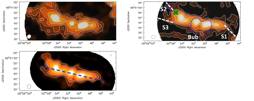
Figure 1.— The integrated intensity maps for ¹²CO(1-0) (upper left panel; Matsushita et al., 2000, 2005), ¹²CO(2-1) (upper right panel) and ¹²CO(3-2) (lower left panel). Numerous features from Walter et al. (2002) and Matsushita et al. (2000) are marked on the ¹²CO(2-1) map. These features include the western spur (S1), the northeastern spur (S2), the southeastern spur (S3), and the expanding super-bubble (bub; outlined in blue). The green X marks the approximate location of a strong knot of [Fe II] emission from Figure 14. The blue regions illustrate the areas used to define the bubble (central structure; from the -85 km s^-1 channel map), and the S2 streamer (northeastern rectangular shape; from the velocity map). S1 and S3 are detected off the south west and east of the disc, respectively, in ¹²CO(2-1) and ¹²CO(3-2), but the ¹²CO(1-0) is not deep enough to detect these features. The blue dashed line on the ¹²CO(3-2) map represents the position slice for the position-velocity diagrams. The beam size of $3\farcs 88\times 3\farcs 32$ (68 pc$\times$58 pc) at a position angle of -32^∘ is indicated in the lower left corner of each panel. The contour levels are 450, 600, 750, 1050, 1500, and 2250 K km s^-1, and the estimated $1\sigma$ intensity errors are 103, 55, and 64 K km/s for the ¹²CO(1-0), ¹²CO(2-1), and ¹²CO(3-2) maps, respectively.

2.2. NMA Observations

The Nobeyama Millimeter Array (NMA) observed M 82 in ¹²CO(1-0) between November 1997 and March 1999, and the full reduction details are given in Matsushita et al. (2000). The NMA data has a velocity resolution of 5.2 km s^-1, a beam size of $2\farcs 8\times 2\farcs 3$ at $-50^{\circ}$, and a pixel size of $0\farcs 25$. Similar to the SMA data above, a primary beam correction is made, and a zeroth moment map is created by integrating between $-180$ and $+150$ km s^-1. We make short-spacing corrections, similar to the ¹²CO(2-1) and ¹²CO(3-2) maps, with a 9% difference between the single dish data (Weiß et al., 2005) and the NMA data. Finally, the zeroth moment map is convolved to the resolution of the ¹²CO(2-1) map.

2.3. HST [Fe II] Imaging

We use archival Hubble Space Telescope [Fe II] 1.6 $\mu$m images to determine whether the gas is shocked (Alonso-Herrero et al., 2003). The NICMOS images have a field of view of 53$\farcs$8 by 66$\farcs$2, and a resolution of 0$\farcs$35, more than adequate to compare to the CO observations. The images are reduced using the NicRed package (McLeod, 1997), flux calibrated, and continuum subtracted using off-band F164N images (Alonso-Herrero et al., 2003).

3. RESULTS

Here we present the results of the CO and [Fe II] emission maps. We first introduce the CO intensity, velocity, position-velocity, channel, and line ratio maps (§ 3.1). We then model H₂ temperature and density maps using a Bayesian approach (§ 3.2). Finally we use the [Fe II] emission to locate shocked gas within M 82 (§ 3.3).

3.1. Moment, Channel, and Line Ratio Maps

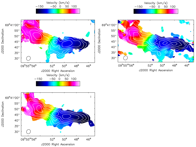
Figure 2.— Maps of the intensity weighted velocity relative to the local standard of rest (225 km s^-1) for ¹²CO(1-0) (top left panel), ¹²CO(2-1) (top right panel), and ¹²CO(3-2) (bottom panel). Only pixels with 5$\sigma$ or greater detections are used to create the map. The S2 and bubble features are both kinematically distinct from the nearby disc (see the red and orange amongst pink for S2, and light blue amongst dark blue for the super-bubble). S2 is blueshifted by $37$ km s^-1, and the bubble is blueshifted by $50$ km s^-1 relative to the rotating disc. The contours are from the zeroth moment maps (Figure 1), and the beam size (68 pc$\times$58 pc at the distance of M 82) is given in the lower left corner.

Figure 3.— The position-velocity diagram for ¹²CO(1-0) (top left panel), ¹²CO(2-1) (top right panel), and ¹²CO(3-2) (bottom left panel) along the dashed blue line in Figure 1. Zero velocity is defined as the velocity of the local standard of rest, or 225 km s^-1. A deviation from rigid body rotation is seen near a position of $0^{\prime\prime}$ (9^h55^m51.0^s, +69${}^{\circ}40^{\prime}44.85^{\prime\prime}$), corresponding to the expanding super-bubble. The emission from the bubble is concentrated between velocities of $-10$ km s^-1 and $-139$ km s^-1. The velocity gradient used to calculate the mass outflow rate of the bubble is given as the solid light-blue line in the ¹²CO(2-1) panel (upper right; see § 4.2). The velocity resolution is 5 km s^-1.

A zeroth moment map measures the integrated intensity in each pixel, and the maps for the three CO emission lines are shown in Figure 1. To measure the standard deviation of the zeroth moment maps, we first measure the standard deviation in the individual channels, then multiply by the velocity resolution (5 km s^-1) and the square root of the number of channels. The zeroth moment $1\sigma$ errors are 103, 55, and 64 K km s^-1 for the ¹²CO(1-0), ¹²CO(2-1), and ¹²CO(3-2) maps, respectively. Three distinct intensity peaks are seen (Shen & Lo, 1995; Weiß et al., 2001; Walter et al., 2002), and four previously observed large-scale features are detected: three molecular spurs off the disc (named S1, S2, S3; Walter et al., 2002), and an expanding super-bubble (Weiß et al., 1999; Matsushita et al., 2000).

The intensity weighted velocity maps (also called the first moment maps) are shown in Figure 2. Galactic rotation is seen across the disc, with the velocity steadily increasing from east to west. The rotational center of the galaxy resides between the left two peaks in Figure 1, while an evolved 10⁶ M_⊙ super star cluster is between the right two CO intensity peaks (Matsushita et al., 2000).

Slicing the image cube along the dashed blue line in the bottom panel of Figure 1, we produce the position-velocity (PV) diagrams for each transition (Figure 3). A PV diagram plots the intensity at a particular position and velocity, and diagnoses the kinematics of the gas. The PV diagrams show a steady decrease in velocity with increasing position (i.e., rigid rotation). Near the $0^{\prime\prime}$ position the CO deviates from the rigid rotation. Matsushita et al. (2000) attribute this abrupt change in velocity to an expanding molecular super-bubble.

We also use the channel maps – or the intensity within a given velocity interval – to study the distribution of CO gas in velocity space. Figures 4, 5 and 6 show the channel maps for ¹²CO(1-0), ¹²CO(2-1), and ¹²CO(3-2), respectively. We define six channels, separated by 55 km s^-1, with median velocities given in the upper right corners of each map. The $-195$ km s^-1, $-140$ km s^-1, $-30$ km s^-1, and $+80$ km s^-1 channels largely contain disc emission. The $-85$ km s^-1 channel (middle left panel) has emission from the super-bubble, and the area defined by this feature is shown by the blue circle in the upper right panel of Figure 1. Moreover, we detect the S2 streamer from Walter et al. (2002) in the upper left corner of the $+25$ km s^-1channel (lower left panel). The ¹²CO(2-1) and ¹²CO(3-2) lines show more streamers: S1 is seen in the bottom right of the $-140$ km s^-1 channel and in the lower right of the ¹²CO(3-2) PV diagram. Additionally, S3 is seen in the bottom left of the $+80$ km s^-1 channel (bottom left panel). Unfortunately, the sensitivity of the ¹²CO(1-0) observations from Matsushita et al. (2000) do not afford detections of these diffuse features.

In § 3.2 we use the radiative transfer code RADEX and the line ratios to model the temperatures and densities of the molecular gas in M 82. Figure 7 shows the ¹²CO(2-1)/¹²CO(1-0), ¹²CO(3-2)/¹²CO(1-0), and the ¹²CO(3-2)/¹²CO(2-1) line ratio maps. Additionally, in Table 3 we tabulate the CO emission lines for five regions discussed in § 4. These line ratios provide the basis to model the physical properties of the molecular gas. To calculate the errors on these line ratio maps we must consider the dominant uncertainties in our calibration procedure, which are the calibration errors (short-spacing corrections), not the statistical uncertainties. Therefore, for the line ratio errors we use a calibration uncertainty of 15% and an uncertainty due to our ad hoc short-spacing correction. We make a point-by-point comparison between single dish data from Weiß et al. (2005), Wilson et al. (2012), and Leroy et al. (2015) to our line ratios and find a 20% variation. We conservatively attribute this 20% variation to the ad-hoc prescription for the short-spacing correction. We then add the short-spacing error in quadrature with the 15% calibration uncertainty to find an uncertainty of 25% on the individual line ratios. This is the uncertainty that we model the temperatures and densities with, below.

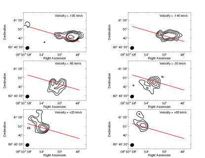
Figure 4.— Channel maps for the ¹²CO(1-0) emission. The six velocity channels are separated by 55 km s^-1, with median velocity given in the top right corner of each map. Zero velocity is defined as the velocity of the local standard of rest (225 km s^-1). The contour levels represent a 7, 10, 15, 20, 40$\sigma$ detection significance. The red-line is the line used to produce the PV diagrams (see Figure 1), and represents the major axis of the galaxy

. The beam size is given in the lower left corner, and is 68 pc$\times 58$ pc at the distance of M 82.

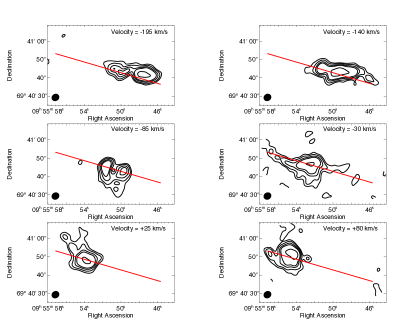
Figure 5.— Same as Figure 4 but for the ¹²CO(2-1) emission.

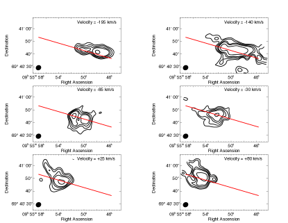
Figure 6.— Same as Figure 4, but for the ¹²CO(3-2) emission.

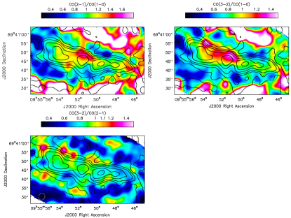
Figure 7.— The CO line ratio maps used to model the molecular temperatures and densities. Only 1$\sigma$ detections are included in the map. The upper left panel is the ¹²CO(2-1)/¹²CO(1-0) ratio, the upper right panel is the ¹²CO(3-2)/¹²CO(1-0) ratio, and the lower left panel is the ¹²CO(3-2)/¹²CO(2-1) ratio. Table 3 tabulates the ratios for five different regions, with points in the disc, the super-bubble, and S2. The black contours are the ¹²CO(2-1) contour levels from Figure 1, and the beam size (68 pc$\times$58 pc) is shown in the lower left corner.

Table 2RADEX Model Parameter Ranges

Parameter	Range	Step Size
Temperature [K]	15 – 295	10
log($n_{\text{H2}}$) [cm-3]	1 – 5	0.1
log($N_{\text{CO}}$) [cm-2]	17 – 23	0.1

Note. — Grid of parameters used to create the RADEX models.

Table 3Line Ratios

Feature	R.A. (2000)	Decl. (2000)	12CO(2-1)/12CO(1-0)	12CO(3-2)/12CO(1-0)	12CO(3-2)/12CO(2-1)	$\tau_{10}$	$\tau_{21}$	$\tau_{32}$
	(hh:mm:ss)	(hh:mm:ss)
Disc	09:55:52.4	+69:40:46.08	$1.17\pm 0.29$	$1.10\pm 0.28$	$0.94\pm 0.24$	10	36	73
Shocked Bubble	09:55:51.0	+69:40:44.82	$0.62\pm 0.16$	$0.80\pm 0.2$	$1.30\pm 0.33$	10	39	79
Outer Bubble	09:55:50.9	+69:40:36.62	$0.38\pm 0.10$	$0.33\pm 0.08$	$0.89\pm 0.22$	33	120	226
Shocked S2	09:55:55.4	+69:40:55.90	$0.80\pm 0.2$	$0.78\pm 0.20$	$0.98\pm 0.25$	58	194	327
S2 Body	09:55:56.2	+69:41:00.00	$0.59\pm 0.15$	$0.57\pm 0.14$	$0.96\pm 0.24$	32	105	176

Note. — Table of CO line ratios for five points in M 82. The errors on the line ratios are 25%, as outlined in § 3.1. The individual points correspond to: the 2 $\mu$m peak position (disc; Lester et al., 1990), a shocked portion of the super bubble, a position further out in the southern bubble (outer bubble), the location of [Fe II] emission at the intersection of S2 and the disc (shocked S2), and a position in the body of S2. The ratios for the disc are calculated using the integrated intensity maps, while the bubble and S2 ratios are calculated only with the $-85$ km s^-1 and $+25$ km s^-1 channel maps. The final three columns give the RADEX modeled optical depths for the ¹²CO(1-0), ¹²CO(2-1), and ¹²CO(3-2) transitions, respectively.

3.2. Density and Temperature Modeling

To model the molecular gas temperatures and densities, we compare the ratios of the ¹²CO(1-0), ¹²CO(2-1), and ¹²CO(3-2) intensities to theoretical ratios from RADEX (van der Tak et al., 2007). RADEX is a one-dimensional, non-LTE, radiative transfer code that calculates the molecular line ratios using an escape probability formulation. RADEX requires inputs of temperature, H₂ density ($n_{\text{H2}}$), CO column density ($N_{\text{CO}}$), and the FWHM of the CO line. We fit the line widths at each pixel for each transition, and find a median FWHM of 89 km s^-1. By using the FHWM of the entire galaxy for the RADEX modeling, we assume that the CO emitting gas is in a single zone, or the entire galaxy is treated as a single cloud of molecular gas. We make this assumption to simplify the Bayesian parameter grid below.

We then create a large grid of RADEX models using the parameters listed in Table 2, and tabulate the predicted line ratios for each input parameter. The RADEX grid is centered on the warm diffuse molecular temperatures and densities found in Weiß et al. (2005), but the grid also allows for very cold dense clouds and the 272 K molecular phase from H₂ rotational transitions (Beirão et al., 2015). We use a Bayesian analysis to calculate the probability of each RADEX model given the observed line ratios (¹²CO(2-1)/¹²CO(1-0), ¹²CO(3-2)/¹²CO(2-1), and ¹²CO(3-2)/¹²CO(1-0)), where only locations detected at greater than 1$\sigma$, for all three lines, are used. We create probability density functions (PDFs) for each marginalized parameter by assuming a flat prior, such that each value is equally likely, and compute the likelihood function as (Brinchmann et al., 2004; Kauffmann et al., 2003; Feigelson & Jogesh Babu, 2012):

$$L\propto\mathrm{exp}(-\chi^{2}/2).$$ (1)

The intensity errors (used in the $\chi^{2}$ function) are 25% from the calibration and short-spacing correction (see § 3.1). The likelihood functions are then normalized, and marginalized over nuisance parameters to produce PDFs for $n_{\text{H2}}$, temperature, and $N_{\text{CO}}$ individually. The PDFs are typically narrowly peaked, and clustered near a single value (see Figure 8), although the temperature PDFs occasionally are broader. The expectation values and standard deviations are calculated from the PDFs. Figure 8 gives a representative example of the three PDFs, the expectation values, and standard deviations from a single pixel within the hot super-bubble region of the $-85$ km s^-1 channel.

Figure 8.— Example probability density functions (PDFs) for a single pixel within the -85 km s^-1 channel (the hot region of the super-bubble). Each panel gives the normalized probability of the model given the observed line ratios. The different panels correspond to the PDFs for the temperature (top panel), the molecular Hydrogen number density (middle panel), and CO column density (bottom panel). The temperature, Hydrogen density (log($n_{\mathrm{H2}}$)), and CO column density (log($N_{\mathrm{CO}}$)) derived from these PDFs are $222\pm 22$ K, $1.79\pm 0.18$ dex, and $20.50\pm 0.50$ dex, respectively.

We plot expectation value maps for the temperature and $n_{\text{H2}}$ over the entire field of view in Figure 9. The log($n_{\text{H2}}$) ranges between 1.8 and 3.1 dex, and temperatures range between 61 and 175 K. The median individual standard deviations of the temperatures and densities are 70 K and 0.66 dex, respectively. Figures 10 and 11 show the temperatures and densities modeled from the channel maps, showing the conditions within specific features, like the super-bubble and S2.

Additionally, we show the relationship between the modeled temperatures and densities (Figure 12). We over-plot curves of constant ¹²CO(2-1)/¹²CO(1-0) and ¹²CO(3-2)/¹²CO(1-0) line ratios from the RADEX models, using a constant log($N_{\mathrm{CO}}$) of 19 dex. In Figure 13 we show the curves corresponding to the same constant line ratios, but for a log($N_{\mathrm{CO}}$) of 19.3, twice the column density in Figure 12. While both the ¹²CO(2-1)/¹²CO(1-0) and ¹²CO(3-2)/¹²CO(2-1) change by changing $N_{\mathrm{CO}}$, the ¹²CO(2-1)/¹²CO(1-0) moves to lower temperatures and densities more rapidly than the ¹²CO(3-2)/¹²CO(2-1). This relation allows for low ¹²CO(2-1)/¹²CO(1-0) yet high ¹²CO(3-2)/¹²CO(2-1) ratios seen in the outer bubble and the S2 body to correspond to low N_CO values (see Table 3). This allows for the $N_{\mathrm{CO}}$ values to be modeled by marginalizing over the PDFs.

The RADEX modeling also provides estimates of the optical depth for each transition. In Table 3 we show the optical depth for each transition in five regions that are discussed below. These optical depths are moderately high and consistent with optical depths derived from single-dish data (Leroy et al., 2015). Observations of optically thin tracers could be used in future studies to provide better estimates of the optical depths (¹³CO(1-0) for example; see Weiß et al. 2005).

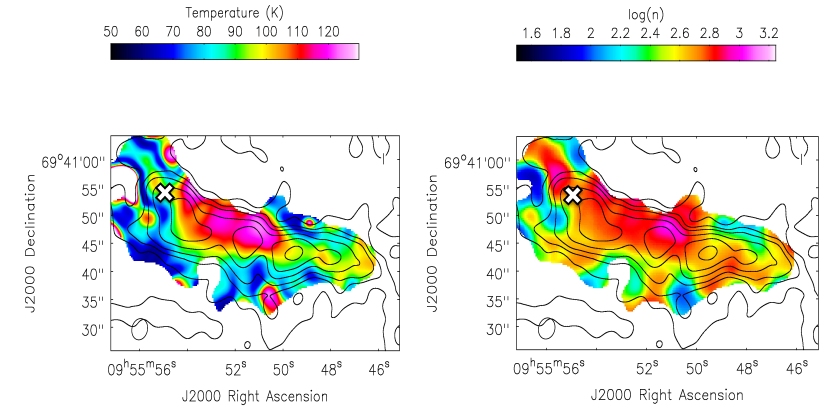
Figure 9.— Maps of the expectation values for the H₂ temperature (left; given in K) and density (right; given in log(cm^-3)). The ¹²CO(2-1) contour map from Figure 1 is overlaid in black to give a sense of position. The white X’s mark the approximate location of the [Fe II] emission from § 3.3.

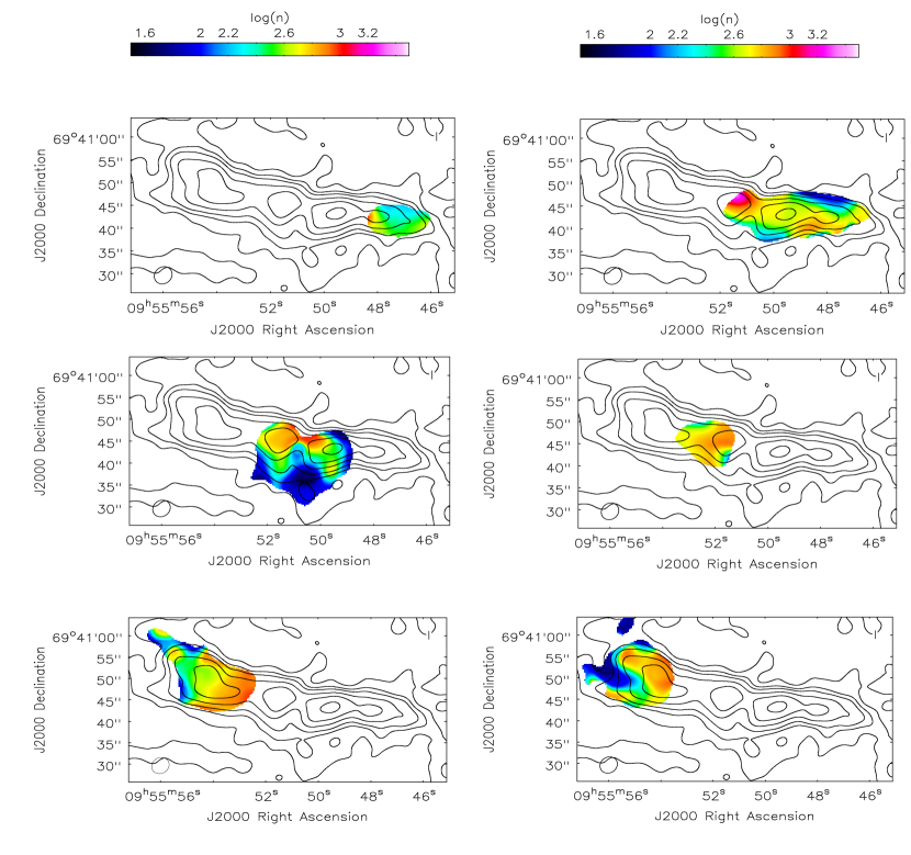
Figure 10.— Density channel maps with the ¹²CO(2-1) contours from Figure 1 overlaid to give a sense of position. The density is only displayed if the three CO lines are detected at more than a 1$\sigma$ significance level. The six maps are the same velocities as Figure 4: $-195$ km s^-1, $-140$ km s^-1, $-85$ km s^-1, $-30$ km s^-1, $+25$ km s^-1, and $+80$ km s^-1. S2 is seen in the $+25$ km s^-1 channel (lower left), and the bubble region is seen in the $-85$ km s^-1 channel (middle left).

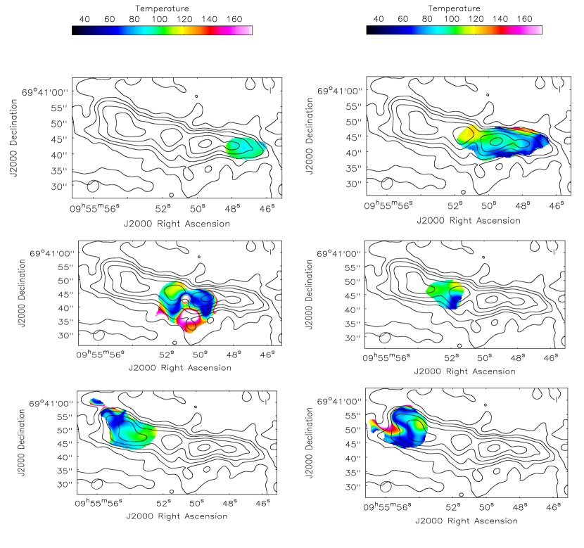
Figure 11.— Same as Figure 10, but for the H₂ temperature.

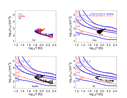
Figure 12.— A random sampling of pixels in the temperature-density plane for the full field of view (upper left), disc (upper right), bubble (lower left) and the S2 region (lower right). In the full field of view, we have color-coded the pixels by whether they are in the disc (gray), the super-bubble (red), or the S2 molecular streamer (blue). Lines of constant ¹²CO(2-1)/¹²CO(1-0) (blue lines) and ¹²CO(3-2)/¹²CO(2-1) (red dashed lines) ratios are shown in the single component panels, created using a constant log($N_{\mathrm{CO}}$[cm^-2]) = 19. The constant ratio lines are labeled near the lowest temperature of each curve.

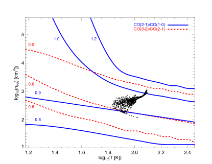
Figure 13.— Same as the disc panel from Figure 12 (upper right), but for a log($N_{\mathrm{CO}}$) = 19.3 (twice the column density of Figure 12). Generally, increasing log($N_{\mathrm{CO}}$) shifts these curves to lower densities, but the ¹²CO(2-1)/¹²CO(1-0) ratio evolves more rapidly than the ¹²CO(3-2)/¹²CO(2-1). $N_{\mathrm{CO}}$ can then be estimated by marginalizing over the density and temperature.

3.3. Shocked Gas

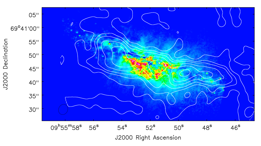
Figure 14.— HST [Fe II] emission map, overlaid with white ¹²CO(2-1) contours from Figure 1. Knots of [Fe II] emission are near the intersection of S2 (upper left portion of the disc), and along the starburst driven bubble.

[Fe II] is a forbidden transition, and requires densities greater than 10⁴ cm^-3 to populate the upper energy state (Mouri et al., 1990). Fast (>100 km s^-1) shocks create high temperatures and densities that collisionally excite Fe II, producing [Fe II] emission in the infrared (Mouri et al., 1990). [Fe II] is less susceptible to dust extinction than optical shock tracers (like [N II]) because of the lower dust attenuation in the infrared. Below, we primarily use these favorable characteristics to determine whether the molecular gas is shocked where S2 intersects the disc.

Figure 14 shows the [Fe II] emission map. The [Fe II] emission strongly peaks near the center of M 82, but the emission also traces the increased density enhancements and depressed temperatures of the super-bubble seen in the $-85$ km s^-1 channel of Figure 10. Intriguingly, there are knots of emission near the intersection of S2 and the disc (see the green X in Figure 1 and Figure 9 for the approximate location of this feature).

4. DISCUSSION

Here we discuss three intriguing physical regions in the CO observations that probe the three phases of the baryon cycle: (1) the disc (§ 4.1) (2) the expanding super-bubble (§ 4.2), and (3) the base of the S2 molecular streamer (§ 4.3). In each section we describe the region, its derived physical properties, how these properties compare to previous observations, and the mass of the feature. Finally, in § 4.4 we discuss how the three areas illustrate the baryon cycle within M 82.

4.1. The Disc

The molecular disc of M 82 is well studied (Weiß et al., 1999; Mao et al., 2000; Matsushita et al., 2000, 2005; Weiß et al., 2001; Walter et al., 2002; Weiß et al., 2005; Keto et al., 2005; Salak et al., 2013; Leroy et al., 2015), and here we use our observations to calculate the molecular gas mass of the disc. We define the disc as the area within the 15$\sigma$ contours of the ¹²CO(2-1) intensity map. We make this distinction to avoid contributions from the super-bubble and the molecular streamers, but it affects comparisons with other studies. To compare the total mass directly with previous studies, we also calculate the total mass within the 450 K km s^-1 ($\approx$3$\sigma$) contours of the ¹²CO(1-0) map, which accounts for all of the observed CO.

The disc has a mean temperature of $104~{}\pm~{}36$ K, and log($n_{\text{H2}}$[cm^-3]) of $2.6\pm 0.5$ dex. These values are consistent with values from Weiß et al. (2001) who use the IRAM Plateau de Bure Interferometer to derive mean temperatures and densities of $125\pm 50$ K and $3.4\pm 0.5$ dex, respectively.

We calculate the total H₂ mass in two ways: (1) by converting the ¹²CO(1-0) intensity into a total molecular mass using an $X_{\mathrm{CO}}$ factor, and (2) by using the CO column densities ($N_{\mathrm{CO}}$) from the RADEX calculations. Method 1 is primarily used to compare with previous results which use a constant $X_{\mathrm{CO}}$ (Matsushita et al., 2000; Weiß et al., 2001; Walter et al., 2002), while the second method uses all three transitions and the radiative transfer analysis to calculate the total H₂ mass. We focus on the results from method 2 while discussing the baryon cycle because it incorporates more of the known physics.

Figure 15.— Map of the $X_{\mathrm{CO}}$ factor (in units of 10¹⁹ cm^-2/(K km s^-1)), as calculated using the RADEX models and Equation 4 (Sakamoto, 1999). The median $X_{\mathrm{CO}}$ factor in the disc is 4$\times$10¹⁹ cm^-2(K km s^-1)^-1, nearly an order of magnitude lower than the Galactic $X_{\mathrm{CO}}$ value. The contours are the ¹²CO(2-1) zeroth moment map from Figure 1, and the beam size(68 pc$\times$ 58 pc) is given in the lower left.

Table 4Mass Calculations

(1)	(2)	(3)	(4)	(5)	(6)	(7)	(8)
Component	$A$	<$I_{10}$>	log10($N_{\mathrm{CO}}$)	log10($M_{H2}$) 1	log10($M_{H2}$) 2	$\nabla$	$\dot{M}$
	(pc2)	(K km s-1)	(cm-2)	(M⊙)	(M⊙)	(10-7yr-1)	(M⊙ yr-1)
Total	395467	831	20.10	8.96	8.32	–	–
Disc	137702	1199	20.30	8.67	8.06	–	–
Bubble	77368	503	19.68	8.04	7.19	10.6	17.1
S2	5650	708	19.81	7.41	6.18	9.03	1.4

Note. — Table of the values used to calculate the total mass of the individual components: the total field of view, the disc, the super-bubble, and the base of the S2 streamer. Column 2 gives the area of each feature (using 17.5 pc per arcsecond). Column 3 gives the average ¹²CO(1-0) intensity of the region, and column 4 gives the ¹²CO column density, calculated with RADEX (see § 3.2). Column 5 gives the total molecular mass from method 1 (see Equation 2), and Column 6 gives the total molecular mass using method 2 (see Equation 3). Column 7 gives the velocity gradient derived from the PV diagram (only for the bubble and S2). Column 8 gives the mass outflow (inflow) rate, calculated using the mass from method 2 (column 6). For these calculations we assume a CO-to-H₂ abundance ratio of $5\times 10^{-5}$ (see Table 5).

Table 5Constants Used in Mass Calculations

Constant	Value	units
$\bar{m}$	$1.96\times 10^{-57}$	M⊙/H2
$X_{CO}$	$1.5\times 10^{20}$	cm${}^{-2}(K~{}$km s${}^{-1})^{-1}$
Z[CO]	$5\times 10^{-5}$	CO/H2
$\Delta$ V	89	km s-1

Note. — Constants used to calculate masses.

Method 1 calculates the total H₂ mass as

$$M=X_{CO}<I_{10}>A\bar{m}$$ (2)

where $X_{\mathrm{CO}}$ converts the median ¹²CO(1-0) intensity ($<I_{10}>$) into a H₂ column density, $A$ is the area of the region (in cm²), and $\bar{m}$ is the average mass per H₂ molecule (see Table 5). To compare to previous studies (Matsushita et al., 2000; Weiß et al., 2001; Walter et al., 2002; Keto et al., 2005), we use an $X_{\mathrm{CO}}$ value that is half the Milky Way value (Solomon et al., 1987, Table 5). Using Method 1, the total H₂ mass within the 3$\sigma$ ¹²CO(1-0) contours is $9\times 10^{8}$ M_⊙ (see Table 4), similar to the $7\times 10^{8}$ M_⊙ Weiß et al. (2001) and Walter et al. (2002) calculate using the $X_{\mathrm{CO}}$ method.

Method 2 uses the RADEX derived $N_{\mathrm{CO}}$ to calculate the total H₂ mass as

$$M=\frac{N_{CO}A\bar{m}}{\Delta VZ[CO]}$$ (3)

where $\Delta V$ is the FWHM (89 km s^-1) and $Z[CO]$ is the CO-to-H₂ abundance ratio (see Table 5; Sakamoto, 1999). The total molecular gas mass within the field of view is 2.1$\times 10^{8}$ M_⊙ (see the first row of column 6 in Table 4), similar to the $2.7\times 10^{8}$ M_⊙ (Weiß et al., 2001) estimated using an LVG solution.

In the disc, there are $5\times 10^{8}$ M_⊙ and $1\times 10^{8}M_{\odot}$ of H₂, using methods 1 and 2, respectively (see Table 4). The two methods differ largely because the excitation of CO depends on the temperature and density of the gas. For example, the $X_{\mathrm{CO}}$ of an optically thick cloud in virial equilibrium scales as $T^{-1}n_{H2}^{1/2}$ (Maloney & Black, 1988; Weiß et al., 2001), and high H₂ temperatures within the disc decrease the conversion factor (Weiß et al., 2001; Bolatto et al., 2013; Leroy et al., 2015). Higher temperatures excite higher energy transitions (¹²CO(3-2) for example), causing the ¹²CO(1-0) transition to trace a lower fraction of the total H₂. This relation only holds for clouds in virial equilibrium, and is meant to illustrate possible ways to decrease $X_{\mathrm{CO}}$. Keto et al. (2005) use high resolution ORVO ¹²CO(2-1) observations and this $X_{\mathrm{CO}}$ value to show that the CO clouds are approximately in virial equilibrium, but it is unlikely that all of the diffuse gas (scales of kpc) in M 82 is in virial equilibrium. To illustrate how the $X_{\mathrm{CO}}$ value changes, we use equation 1 from Sakamoto (1999) to calculate the $X_{\mathrm{CO}}$ value within the disc as

$$X_{CO}=\frac{N_{CO}}{\Delta V~{}Z[CO]<I_{10}>}$$ (4)

In Figure 15 we find that the median disc value is $4.0\times 10^{19}$ cm^-2/(K km/s), roughly consistent with the $X_{\mathrm{CO}}$ factor derived by Weiß et al. (2001) using the LVG method. However, this $X_{\mathrm{CO}}$ factor is 4 times smaller than the value assumed in method 1, and almost an order of magnitude lower than the Milky Way value. The total mass is easily over-estimated if a constant $X_{\mathrm{CO}}$ factor is assumed, especially in regions with high temperatures and densities.

In summary, we calculate the total H₂ mass in two ways: with a constant conversion factor and with our radiative transfer calculations (see Table 4 for the values). Both methods are consistent within a factor of 2 with previous studies. We calculate the $X_{\mathrm{CO}}$ factor within the disc and find that it is also consistent with other studies that use radiative transfer techniques, however it is up to a factor of 4 lower than the constant value typically assumed. We now compare the total H₂ mass within the disc to the mass of the starburst driven super-bubble.

4.2. The Starburst Driven Bubble

The next feature that we discuss is the molecular super-bubble. At the center of the molecular bubble is an evolved 10⁶ M_⊙ super-star cluster dominated by red super-giants. An estimated $4\times 10^{3}$ supernovae have exploded throughout the lifetime of the cluster (Matsushita et al., 2000). This energy and momentum has created an X-ray emitting plasma (Griffiths et al., 2000; Matsushita et al., 2005) that adiabatically expands along the minor axis of the galaxy, and accelerates the cold molecular gas to velocities that reach $-139$ km s^-1(see Figure 3). The $-85$ km s^-1 channel maps (middle left panels in Figures 10 and 11) show that the super-bubble has two components: (1) a moderate density and temperature shell that traces the [Fe II] emission in Figure 14 and (2) a high temperature, low density flow. The temperature and log($n_{\text{H2}}$[cm^-3]) in the shell are $82\pm 17$ K and $2.64\pm 0.18$ dex, while the warm flow has a temperature of $159\pm 30$ K and log($n_{\text{H2}}$[cm^-3]) of $1.93\pm 0.15$ dex, significantly warmer and more rarefied than the disc. The dense shell is coincident with the strong [Fe II] emission (Figure 14), indicating that shocks have compressed the H₂ to form the dense shell.

Similar to the molecular disc, we calculate the total mass of the bubble in two ways using Equation 2, Equation 3, and the values from Table 4. To calculate the mass of the super-bubble we use the intensity and $N_{\mathrm{CO}}$ found within the $-85$ km s^-1 channel. This channel maximizes the emission from the bubble, while minimizing the contributions from the disc (see § 3.1). The total mass in the super-bubble is $1.1\times 10^{8}M_{\odot}$ for method 1. Using a similar $X_{\mathrm{CO}}$ factor, Matsushita et al. (2000) find a total molecular mass of $1.8\times 10^{8}$ M_⊙. Using method 2 we find a total H₂ mass of $1.5\times 10^{7}M_{\odot}$, 7% of the total H₂ mass within the galaxy.

We calculate the mass outflow rate using the velocity gradient from the PV diagram (see Figure 3). The bubble initially expands nearly isotropically because it is not pressure-confined by the disc, as shown by the shell-like structure in the position-velocity diagram. This isotropic expansion velocity corresponds to the velocity of the molecular outflow (Matsushita et al., 2000). The velocity gradient ($\nabla$) of the bubble extends from $-8$$\farcs$10 to 0$\farcs$76, with velocities from $-10$ to $-139$ km s^-1. Using the conversion factor that 1$\farcs$0 is 17.5 pc, we calculate $\nabla$ as

$$\nabla=\frac{\Delta v}{\Delta D}$$ (5)

with a value of $1.1\times 10^{-6}$ yr^-1. The total mass outflow rate ($\dot{M}$) is given by:

$$\dot{M}=M\nabla$$ (6)

for a $\dot{M}$ of 17 M_⊙ yr^-1, using the mass from method 2. We do not calculate $\dot{M}$ for method 1 because the discrepancies associated with a constant X_CO factor (see § 4.1).

Interestingly, the molecular mass outflow rate is similar to the large-scale atomic and ionized mass outflow rate calculated using the [O I] and [C II] emission lines (Contursi et al., 2013). However, the molecular, neutral, and ionized outflows are in quite different physical locations: the CO emission dominates the inner kpc of the outflow (Walter et al., 2002; Salak et al., 2013; Leroy et al., 2015), while the neutral and ionized emission extends further into the outflow (Shopbell & Bland-Hawthorn, 1998; Leroy et al., 2015). This suggests that the molecular outflow is the base of the galactic outflow. Initially the stellar energy and momentum creates a hot plasma the size of the star-cluster. This hot plasma expands adiabatically and encounters the surrounding dense molecular gas within the disc, shocking and accelerating the molecular gas into the observed shell structure. The hot plasma rapidly heats and dissociates the molecular gas, mixing the cold and hot gas. While the hot outflow initially contains a negligible amount of mass, the added molecular gas significantly increases the mass of the outflow (Chevalier & Clegg, 1985; Heckman et al., 1990; Cooper et al., 2008; Strickland & Heckman, 2009). This “mass-loading” transports cold gas out of the disc and into the halo through the galactic outflow, where it is later observed by warmer tracers like [O I], [C II], H$\alpha$, and metal absorption lines (Heckman et al., 2000; Veilleux et al., 2005; Contursi et al., 2013). Mass-conservation requires that the outflow rate at the base of the outflow (the molecular gas) is equal to the outflow rate at later times and larger distances (the neutral and ionized gas), which is consistent with the observations of the atomic and ionized gas.

X-ray emission probes the mass-loading because it arises in the interaction region between the hot plasma and the molecular gas (Strickland & Stevens, 2000; Cooper et al., 2008). The mass-loading factor ($\eta=\dot{M}_{o}/SFR$) measures the efficiency of the outflow, relative to the star formation rate. With a star formation rate of 13 $M_{\odot}$ yr^-1 (Förster Schreiber et al., 2003), M 82 has a molecular mass-loading factor of 1.3. Models of the X-ray Fe and S line fluxes of M 82 find that the mass-loading factor must be between 1.0 and 2.8 (Strickland & Heckman, 2009), consistent with the molecular gas mass-loading found here.

After the molecular gas has been ejected from the disc, what is the final location of the gas? Does the molecular gas have enough kinetic energy to overcome gravity, or will the gas fall back as a galactic fountain (Shapiro & Field, 1976)? The two scenarios illustrate very different implications for the baryon cycle: recycled gas can eventually be retained as stars, while escaping gas will decrease the fraction of baryons relative to the dark matter. Using a conservative estimate that the escape velocity is three times the circular velocity (Heckman et al., 2000) and a circular velocity of 136 km s^-1 (Yun et al., 1993), the escape velocity of M 82 is 408 km s^-1, significantly higher than the the CO outflow velocity of 139 km s^-1 from Figure 3. However, dissociated clouds of CO can be accelerated by ram pressure, and the clouds then may approach the escape velocity. Chisholm et al. (2016) find a shallow scaling relation between SFR and the centroid velocity of the Si IV absorption lines (a warm ionized gas tracer). Using 13 M_⊙ yr^-1, these scaling relations predict the Si IV velocity would be 222 km s^-1, implying that the molecular gas must accelerate 87 km s^-1 during the dissociation and ionization process. However, this velocity is still below the escape velocity, and the molecular gas is likely recycled. This result echoes the finding from Leroy et al. (2015) where the radial density profile of the gas and dust are too steep to produce a galactic outflow. The steep density profiles more naturally suggest that M 82’s molecular bubble ends as a galactic fountain rather than a large scale outflow.

4.3. The Bases of the Molecular Streamers

Walter et al. (2002) identify four "streamers" in the wide field CO images. These streamers are large scale structures that extend 2 kpc from the edge of the molecular disc (Salak et al., 2013; Leroy et al., 2015). While we detect S1 and S3 in the ¹²CO(2-1) and ¹²CO(3-2) images, the ¹²CO(1-0) field of view only provides adequate analysis of the base of the S2 streamer (the northeastern streamer). However, S2 is the base of a large H I trailing tail thought to have formed from the interaction of M 82 and M 81 (Yun et al., 1993, 1994). The S2 streamer has the highest H I column density of the observed streamers ($5.6\times 10^{20}$ cm^-2), and an estimated H I mass of $6.4\times 10^{7}M_{\odot}$ (Yun et al., 1993).

S2 is set apart from the disc as a moderately high density and temperature region in the full temperature and density plots (Figure 9). In the +25 km s^-1 channel map (lower left panel of Figure 11), S2 has a log($n_{\text{H2}}$[cm^-3]) of 2.3 dex and a temperature of 128 K. The kinematics of S2 also distinguish it from the disc, with S2 blueshifted $-37$ km s^-1 from the disc (see Figure 2).

Further, in § 3.3 we find that there is a strong knot of [Fe II] at the intersection of S2 and the disc, demonstrating that the gas is shocked at their intersection. The [Fe II] is not the only shock tracer available. Westmoquette et al. (2009a) find elevated [N II]/H$\alpha$ and [S II]/H$\alpha$ ratios near the base of S2, but caution that the elevated ratios could be due to Hydrogen absorption. Finally, García-Burillo et al. (2001) find that the two main sources of SiO in M 82 are the super-bubble, and the “chimney”, a large extended filament out of the disc. Figure 2 of García-Burillo et al. (2001) shows a third source of SiO emission northeast of the main chimney, at a position and velocity consistent with the intersection of S2 and the disc. SiO traces shocked gas because it is released after a shock destroys dust grains (Martin-Pintado et al., 1992). Therefore, the available shock diagnostics indicate that there is a shock at the intersection of S2 and the disc.

The distinct kinematics of S2 suggest that S2 is either an inflowing molecular filament, or a molecular outflow. These two scenarios are distinguished by the geometries of the system: if S2 is on the far side, the blueshifted emission implies that the gas is flowing onto the disc; whereas if S2 is on the near side, the blueshifted emission implies the gas is flowing out of the disc. Three observations lead us to hypothesize that S2 is an inflowing filament. First, if S2 is a molecular outflow there should be a burst of star formation that drives the CO out of the disc. There is not strong 100 GHz (Matsushita et al., 2005), H$\alpha$ (Westmoquette et al., 2009a), Pa-$\alpha$ (Alonso-Herrero et al., 2003), nor X-ray emission (Griffiths et al., 2000) in this region, implying that there is not a large amount of star formation in the vicinity. Secondly, there are strong shock indicators at the intersection of S2 and the disc. Gas flowing into a rotating disc will shock, but CO outflowing from the disc would not. Third, using the measured $N_{\mathrm{CO}}$ column density along S2, the CO-to-H₂ conversion factor, and a Calzetti extinction law (Calzetti et al., 2000), we would expect S2 to extinct the galaxy by an A_V of 28 magnitudes, which is not observed in optical images of S2 (Mutchler et al., 2007). Therefore, we assume that S2 is on the far side of the galaxy, and that S2 is a molecular inflow. In fact, S2 is likely the base of the large-scale gaseous streamer observed in H I that is created through the tidal interactions between M 82 and M 81 (Yun et al., 1993, 1994).

To calculate the molecular gas mass inflow rate, we use the area defined by the kinematically distinct region of the ¹²CO(2-1) velocity map (see the velocity map in Figure 2, and Figure 1 for the blue outline of the region). The total molecular gas mass of the base of S2, using method 1 (Equation 2), is $3\times 10^{7}M_{\odot}$, while the molecular gas mass is $2\times 10^{6}M_{\odot}$ using method 2 (Equation 3). The velocity gradient is measured from the PV diagram, and found to be $9\times 10^{-7}$ yr^-1, for a total molecular gas mass inflow rate of $1.4~{}M_{\odot}$ yr^-1 (see Table 4).

Here, we only observe the molecular accretion, but there are other contributions to the total baryon cycle in M 82. M 82 gains and loses neutral and ionized gas, while dissociation, ionization, and recombination convert the molecular, neutral, and ionized gas into other phases. This leads to a fluid, and complicated, inflow rate. Furthermore, the accretion we probe is only filamentary, and mostly due to the tidal interaction with M 82’s companions. Spherical accretion assuredly occurs in many of the phases. Unfortunately, spherical accretion is difficult to kinematically distinguish from disc gas because the velocities of both are set by the gravity of the galaxy. Therefore, the accretion rate we measure is a lower limit of both the molecular accretion rate and the total accretion rate.

4.4. The Molecular Baryon Cycle

In the past three sections we have outlined how gas is accreted onto (§ 4.3), resides within (§ 4.1), and ejected out (§ 4.2) of the nearby starburst M 82. Additionally, baryons can be locked into stars through star formation, and M 82 is forming stars at a rate of 13 $M_{\odot}$ yr^-1 (Förster Schreiber et al., 2003). This traces the entire molecular baryon cycle. To remain in a steady-state, M 82 requires a molecular inflow rate of 30 $M_{\odot}$ yr^-1 (SFR plus $\dot{M}$), but we only observe a molecular inflow rate of 1.4 $M_{\odot}$ yr^-1 from one – of the four known – molecular streamers.

Yun et al. (1993) find that the S2 streamer contains 40% of the observed H I mass in the streamers. If we assume that the H I is a proxy for the H₂ and that the other streamers accrete onto the disc at the same relative rate as S2, the total inferred molecular inflow rate is 3.5 M_⊙ yr^-1 (1.4 M_⊙ yr^-1/0.4). Using this accretion rate, we find that M 82 is consuming, and expelling molecular gas 9 times faster than it is acquiring molecular gas. The molecular baryon cycle in M 82 is running a deficit: if the current rates continue, M 82 will consume or expel all of the observed molecular gas in 7.8 Myr. With over $3\times 10^{8}$ M_⊙ of H I in and around the galaxy (Yun et al., 1993), converting H I into H₂ may extend this depletion timescale (Krumholz et al., 2008, 2009), but how efficiently H I is converted into H₂ is uncertain. Additionally, ionized gas can recombine and eventually cool to molecular gas, and spherical accretion of ionized gas may provide another source of molecular gas. However, if the molecular gas acquisition rate does not increase in the next 8 Myr, the star formation rate or the outflow rate must decrease, or M 82 will exhaust all of its molecular gas.

5. CONCLUSION

We present ¹²CO(2-1) and ¹²CO(3-2) observations of M 82, a nearby starburst galaxy. We combine these measurements with previous ¹²CO(1-0), and [Fe II] emission lines to illustrate the physical properties of the molecular gas. We calculate the molecular gas mass of three previously identified features: the disc, an expanding super-bubble, and the base of a molecular streamer (named S2). Using the kinematics, shock tracers (SiO emission and [Fe II] emission), and optical extinction, we argue that S2 is an inflowing filament of molecular gas that is shocked as it encounters the disc. We then compare the star formation rate (13 $M_{\odot}~{}$yr^-1), molecular mass outflow rate (17 $M_{\odot}$ yr^-1), and molecular mass inflow rate (3.5 $M_{\odot}$ yr^-1) to find that the molecular gas is consumed more rapidly than it is replenished by the inflow. We conclude that the baryon cycle in M 82 is running a deficit: unless more molecular gas is acquired, the star formation rate or outflow rate must decrease in the next eight million years.

References

- Alonso-Herrero et al. (2003) Alonso-Herrero, A., Rieke, G. H., Rieke, M. J., & Kelly, D. M. 2003, AJ, 125, 1210
- Beirão et al. (2015) Beirão, P., Armus, L., Lehnert, M. D., et al. 2015, MNRAS, 451, 2640
- Bigiel et al. (2008) Bigiel, F., Leroy, A., Walter, F., et al. 2008, AJ, 136, 2846
- Bland & Tully (1988) Bland, J., & Tully, B. 1988, Nature, 334, 43
- Bolatto et al. (2013) Bolatto, A. D., Wolfire, M., & Leroy, A. K. 2013, ARA&A, 51, 207
- Brinchmann et al. (2004) Brinchmann, J., Charlot, S., White, S. D. M., et al. 2004, MNRAS, 351, 1151
- Calzetti et al. (2000) Calzetti, D., Armus, L., Bohlin, R. C., et al. 2000, ApJ, 533, 682
- Chevalier & Clegg (1985) Chevalier, R. A., & Clegg, A. W. 1985, Nature, 317, 44
- Chisholm et al. (2016) Chisholm, J., Tremonti, C. A., Leitherer, C., Chen, Y., & Wofford, A. 2016, ArXiv e-prints, arXiv:1601.05090
- Chisholm et al. (2015) Chisholm, J., Tremonti, C. A., Leitherer, C., et al. 2015, ApJ, 811, 149
- Contursi et al. (2013) Contursi, A., Poglitsch, A., Grácia Carpio, J., et al. 2013, A&A, 549, A118
- Cooper et al. (2008) Cooper, J. L., Bicknell, G. V., Sutherland, R. S., & Bland-Hawthorn, J. 2008, ApJ, 674, 157
- Davé et al. (2011) Davé, R., Finlator, K., & Oppenheimer, B. D. 2011, MNRAS, 416, 1354
- Dekel et al. (2009) Dekel, A., Birnboim, Y., Engel, G., et al. 2009, Nature, 457, 451
- Di Matteo et al. (2005) Di Matteo, T., Springel, V., & Hernquist, L. 2005, Nature, 433, 604
- Feigelson & Jogesh Babu (2012) Feigelson, E. D., & Jogesh Babu, G. 2012, Modern Statistical Methods for Astronomy
- Finlator & Davé (2008) Finlator, K., & Davé, R. 2008, MNRAS, 385, 2181
- Förster Schreiber et al. (2003) Förster Schreiber, N. M., Genzel, R., Lutz, D., & Sternberg, A. 2003, ApJ, 599, 193
- Freedman et al. (1994) Freedman, W. L., Hughes, S. M., Madore, B. F., et al. 1994, ApJ, 427, 628
- García-Burillo et al. (2001) García-Burillo, S., Martín-Pintado, J., Fuente, A., & Neri, R. 2001, ApJ, 563, L27
- Genzel et al. (2010) Genzel, R., Tacconi, L. J., Gracia-Carpio, J., et al. 2010, MNRAS, 407, 2091
- Griffiths et al. (2000) Griffiths, R. E., Ptak, A., Feigelson, E. D., et al. 2000, Science, 290, 1325
- Heckman et al. (1990) Heckman, T. M., Armus, L., & Miley, G. K. 1990, ApJS, 74, 833
- Heckman et al. (2000) Heckman, T. M., Lehnert, M. D., Strickland, D. K., & Armus, L. 2000, ApJS, 129, 493
- Ho et al. (2004) Ho, P. T. P., Moran, J. M., & Lo, K. Y. 2004, ApJ, 616, L1
- Hopkins et al. (2006) Hopkins, P. F., Hernquist, L., Cox, T. J., et al. 2006, ApJS, 163, 1
- Hopkins et al. (2013) Hopkins, P. F., Kereš, D., Murray, N., et al. 2013, MNRAS, 433, 78
- Hopkins et al. (2011) Hopkins, P. F., Quataert, E., & Murray, N. 2011, MNRAS, 417, 950
- Katz et al. (2003) Katz, N., Keres, D., Dave, R., & Weinberg, D. H. 2003, in Astrophysics and Space Science Library, Vol. 281, The IGM/Galaxy Connection. The Distribution of Baryons at z=0, ed. J. L. Rosenberg & M. E. Putman, 185
- Kauffmann et al. (2003) Kauffmann, G., Heckman, T. M., White, S. D. M., et al. 2003, MNRAS, 341, 33
- Kennicutt (1998) Kennicutt, Jr., R. C. 1998, ApJ, 498, 541
- Kereš et al. (2009) Kereš, D., Katz, N., Fardal, M., Davé, R., & Weinberg, D. H. 2009, MNRAS, 395, 160
- Kereš et al. (2005) Kereš, D., Katz, N., Weinberg, D. H., & Davé, R. 2005, MNRAS, 363, 2
- Keto et al. (2005) Keto, E., Ho, L. C., & Lo, K.-Y. 2005, ApJ, 635, 1062
- Krumholz et al. (2008) Krumholz, M. R., McKee, C. F., & Tumlinson, J. 2008, ApJ, 689, 865
- Krumholz et al. (2009) —. 2009, ApJ, 693, 216
- Leroy et al. (2008) Leroy, A. K., Walter, F., Brinks, E., et al. 2008, AJ, 136, 2782
- Leroy et al. (2015) Leroy, A. K., Walter, F., Martini, P., et al. 2015, ApJ, 814, 83
- Lester et al. (1990) Lester, D. F., Gaffney, N., Carr, J. S., & Joy, M. 1990, ApJ, 352, 544
- Lynds & Sandage (1963) Lynds, C. R., & Sandage, A. R. 1963, ApJ, 137, 1005
- Maloney & Black (1988) Maloney, P., & Black, J. H. 1988, ApJ, 325, 389
- Mao et al. (2000) Mao, R. Q., Henkel, C., Schulz, A., et al. 2000, A&A, 358, 433
- Martin (2005) Martin, C. L. 2005, ApJ, 621, 227
- Martin-Pintado et al. (1992) Martin-Pintado, J., Bachiller, R., & Fuente, A. 1992, A&A, 254, 315
- Matsushita et al. (2005) Matsushita, S., Kawabe, R., Kohno, K., et al. 2005, ApJ, 618, 712
- Matsushita et al. (2000) Matsushita, S., Kawabe, R., Matsumoto, H., et al. 2000, ApJ, 545, L107
- McLeod (1997) McLeod, B. A. 1997, in The 1997 HST Calibration Workshop with a New Generation of Instruments, ed. S. Casertano, R. Jedrzejewski, T. Keyes, & M. Stevens, 281
- McMullin et al. (2007) McMullin, J. P., Waters, B., Schiebel, D., Young, W., & Golap, K. 2007, in Astronomical Society of the Pacific Conference Series, Vol. 376, Astronomical Data Analysis Software and Systems XVI, ed. R. A. Shaw, F. Hill, & D. J. Bell, 127
- Mihos & Hernquist (1994) Mihos, J. C., & Hernquist, L. 1994, ApJ, 431, L9
- Moster et al. (2010) Moster, B. P., Somerville, R. S., Maulbetsch, C., et al. 2010, ApJ, 710, 903
- Mouri et al. (1990) Mouri, H., Nishida, M., Taniguchi, Y., & Kawara, K. 1990, ApJ, 360, 55
- Mutchler et al. (2007) Mutchler, M., Bond, H. E., Christian, C. A., et al. 2007, PASP, 119, 1
- Ohyama et al. (2002) Ohyama, Y., Taniguchi, Y., Iye, M., et al. 2002, PASJ, 54, 891
- Oppenheimer & Davé (2008) Oppenheimer, B. D., & Davé, R. 2008, MNRAS, 387, 577
- Peeples et al. (2014) Peeples, M. S., Werk, J. K., Tumlinson, J., et al. 2014, ApJ, 786, 54
- Rupke et al. (2005) Rupke, D. S., Veilleux, S., & Sanders, D. B. 2005, ApJS, 160, 115
- Saintonge et al. (2012) Saintonge, A., Tacconi, L. J., Fabello, S., et al. 2012, ApJ, 758, 73
- Sakamoto (1999) Sakamoto, S. 1999, ApJ, 523, 701
- Salak et al. (2013) Salak, D., Nakai, N., Miyamoto, Y., Yamauchi, A., & Tsuru, T. G. 2013, PASJ, 65, doi:10.1093/pasj/65.3.66
- Shapiro & Field (1976) Shapiro, P. R., & Field, G. B. 1976, ApJ, 205, 762
- Sharp & Bland-Hawthorn (2010) Sharp, R. G., & Bland-Hawthorn, J. 2010, ApJ, 711, 818
- Shen & Lo (1995) Shen, J., & Lo, K. Y. 1995, ApJ, 445, L99
- Shopbell & Bland-Hawthorn (1998) Shopbell, P. L., & Bland-Hawthorn, J. 1998, ApJ, 493, 129
- Solomon et al. (1987) Solomon, P. M., Rivolo, A. R., Barrett, J., & Yahil, A. 1987, ApJ, 319, 730
- Springel et al. (2005) Springel, V., Di Matteo, T., & Hernquist, L. 2005, MNRAS, 361, 776
- Strickland & Heckman (2009) Strickland, D. K., & Heckman, T. M. 2009, ApJ, 697, 2030
- Strickland et al. (2004) Strickland, D. K., Heckman, T. M., Colbert, E. J. M., Hoopes, C. G., & Weaver, K. A. 2004, ApJS, 151, 193
- Strickland & Stevens (2000) Strickland, D. K., & Stevens, I. R. 2000, MNRAS, 314, 511
- Tremonti et al. (2004) Tremonti, C. A., Heckman, T. M., Kauffmann, G., et al. 2004, ApJ, 613, 898
- Tumlinson et al. (2011) Tumlinson, J., Thom, C., Werk, J. K., et al. 2011, Science, 334, 948
- van der Tak et al. (2007) van der Tak, F. F. S., Black, J. H., Schöier, F. L., Jansen, D. J., & van Dishoeck, E. F. 2007, A&A, 468, 627
- Veilleux et al. (2005) Veilleux, S., Cecil, G., & Bland-Hawthorn, J. 2005, ARA&A, 43, 769
- Walter et al. (2002) Walter, F., Weiss, A., & Scoville, N. 2002, ApJ, 580, L21
- Weiß et al. (2001) Weiß, A., Neininger, N., Hüttemeister, S., & Klein, U. 2001, A&A, 365, 571
- Weiß et al. (1999) Weiß, A., Walter, F., Neininger, N., & Klein, U. 1999, A&A, 345, L23
- Weiß et al. (2005) Weiß, A., Walter, F., & Scoville, N. Z. 2005, A&A, 438, 533
- Werk et al. (2014) Werk, J. K., Prochaska, J. X., Tumlinson, J., et al. 2014, ApJ, 792, 8
- Westmoquette et al. (2009a) Westmoquette, M. S., Gallagher, J. S., Smith, L. J., et al. 2009a, ApJ, 706, 1571
- Westmoquette et al. (2009b) Westmoquette, M. S., Smith, L. J., Gallagher, III, J. S., et al. 2009b, ApJ, 696, 192
- Wilson et al. (2012) Wilson, C. D., Warren, B. E., Israel, F. P., et al. 2012, MNRAS, 424, 3050
- Yun et al. (1993) Yun, M. S., Ho, P. T. P., & Lo, K. Y. 1993, ApJ, 411, L17
- Yun et al. (1994) —. 1994, Nature, 372, 530
- Zahid et al. (2014) Zahid, H. J., Dima, G. I., Kudritzki, R.-P., et al. 2014, ApJ, 791, 130