Measurement uncertainty relations for discrete observables: Relative entropy formulation

Abstract

We introduce a new information-theoretic formulation of quantum measurement uncertainty relations, based on the notion of relative entropy between measurement probabilities. In the case of a finite-dimensional system and for any approximate joint measurement of two target discrete observables, we define the entropic divergence as the maximal total loss of information occurring in the approximation at hand. For fixed target observables, we study the joint measurements minimizing the entropic divergence, and we prove the general properties of its minimum value. Such a minimum is our uncertainty lower bound: the total information lost by replacing the target observables with their optimal approximations, evaluated at the worst possible state. The bound turns out to be also an entropic incompatibility degree, that is, a good information-theoretic measure of incompatibility: indeed, it vanishes if and only if the target observables are compatible, it is state-independent, and it enjoys all the invariance properties which are desirable for such a measure. In this context, we point out the difference between general approximate joint measurements and sequential approximate joint measurements; to do this, we introduce a separate index for the tradeoff between the error of the first measurement and the disturbance of the second one. By exploiting the symmetry properties of the target observables, exact values, lower bounds and optimal approximations are evaluated in two different concrete examples: (1) a couple of spin-1/2 components (not necessarily orthogonal); (2) two Fourier conjugate mutually unbiased bases in prime power dimension. Finally, the entropic incompatibility degree straightforwardly generalizes to the case of many observables, still maintaining all its relevant properties; we explicitly compute it for three orthogonal spin-1/2 components.

1 Introduction

In the foundations of Quantum Mechanics, a remarkable achievement of the last years has been the clarification of the differences between preparation uncertainty relations (PURs) and measurement uncertainty relations (MURs) [1, 2, 3, 4, 6, 11, 13, 10, 7, 8, 12, 5, 9], both of them arising from Heisenberg’s heuristic considerations about the precision with which the position and the momentum of a quantum particle can be determined [14].

One speaks of PURs when some lower bound is given on the “spreads” of the distributions of two observables $\mathsf{A}$ and $\mathsf{B}$ measured in the same state $\rho$. The most known formulation of PURs, due to Robertson [15], involves the product of the two standard deviations; more recent formulations are given in terms of distances among probability distributions [10] or entropies [16, 17, 18, 21, 19, 20, 22, 13].

On the other hand, one refers to MURs when some lower bound is given on the “errors” of any approximate joint measurement $\mathsf{M}$ of two target observables $\mathsf{A}$ and $\mathsf{B}$. When $\mathsf{M}$ is realized as a sequence of two measurements, one for each target observable, MURs are regarded also as relations between the “error” allowed in an approximate measurement of the first observable and the “disturbance” affecting the successive measurement of the second one.

Although the recent developments of the theory of approximate quantum measurements [23, 24, 11, 26, 25] and nondisturbing quantum measurements [27, 28] have generated a considerable renewed interest in MURs, no agreement has yet been reached about the proper quantifications of the “error” or “disturbance” terms. Here, the main problem is how to compare the target observables $\mathsf{A}$ and $\mathsf{B}$ with their approximate or perturbed versions provided by the marginals $\mathsf{M}_{[1]}$ and $\mathsf{M}_{[2]}$ of $\mathsf{M}$; indeed, $\mathsf{A}$, $\mathsf{M}_{[1]}$, $\mathsf{M}_{[2]}$ and $\mathsf{B}$ may typically be incompatible. The proposals then range from operator formulations of the error [1, 2, 3, 4, 29, 30] to distances for probability distributions [6, 10, 7, 8, 12, 9, 11] and conditional entropies [31, 32, 33].

In this paper, we propose and develop a new approach to MURs based on the notion of relative entropy. Here we deal with the case of discrete observables for a finite dimensional quantum system. The extension to position and momentum is given in [34].

In the spirit of Busch, Lahti, Werner [6, 10, 7, 8, 9], we quantify the “error” in the approximation $\mathsf{A}\simeq\mathsf{M}_{[1]}$ by comparing the respective outcome distributions $\mathsf{A}^{\rho}$ and $\mathsf{M}_{[1]}^{\rho}$ in every possible state $\rho$; however, differently from [6, 10, 7, 8, 9], the comparison is done from the point of view of information theory. Then, the natural choice is to consider $S\big{(}\mathsf{A}^{\rho}\|\mathsf{M}_{[1]}^{\rho}\big{)}$, the relative entropy of $\mathsf{A}^{\rho}$ with respect to $\mathsf{M}_{[1]}^{\rho}$, as a quantification of the information loss when $\mathsf{A}^{\rho}$ is approximated with $\mathsf{M}_{[1]}^{\rho}$. Similarly, in order to quantify either the “error” or – if $\mathsf{A}$ and $\mathsf{B}$ are measured in sequence – the “disturbance” related to the approximation $\mathsf{B}\simeq\mathsf{M}_{[2]}$, we employ the relative entropy $S\big{(}\mathsf{B}^{\rho}\|\mathsf{M}_{[2]}^{\rho}\big{)}$. Relative entropy appears to be the fundamental quantity from which the other entropic notions can be derived, cf. [35, 36, 37]. It should be noticed that relative entropy, of classical or quantum type, has already been used in quantum measurement theory to give proper measures of information gains and losses in various scenarios [37, 38, 39, 40, 41].

The relative entropy formulation of MURs, given in Section 2.3, is: for every approximate joint measurement $\mathsf{M}$ of $\mathsf{A}$ and $\mathsf{B}$, there exists a state $\rho$ such that

$$S\big{(}\mathsf{A}^{\rho}\|\mathsf{M}^{\rho}_{[1]}\big{)}+S\big{(}\mathsf{B}^{\rho}\|\mathsf{M}^{\rho}_{[2]}\big{)}\geq c(\mathsf{A},\mathsf{B}),$$ (1)

where the uncertainty lower bound

$$c(\mathsf{A},\mathsf{B})=\inf_{\mathsf{M}}\sup_{\rho}\Big{\{}S\big{(}\mathsf{A}^{\rho}\|\mathsf{M}^{\rho}_{[1]}\big{)}+S\big{(}\mathsf{B}^{\rho}\|\mathsf{M}^{\rho}_{[2]}\big{)}\Big{\}}$$ (2)

depends on the allowed joint measurements $\mathsf{M}$. In the above definition, the same state $\rho$ appears in both error terms $S\big{(}\mathsf{A}^{\rho}\|\mathsf{M}^{\rho}_{[1]}\big{)}$ and $S\big{(}\mathsf{B}^{\rho}\|\mathsf{M}^{\rho}_{[2]}\big{)}$; thus, by making their sum, all possible error compensations are taken into account in the maximization. The quantity $\sup_{\rho}\left\{S\big{(}\mathsf{A}^{\rho}\|\mathsf{M}^{\rho}_{[1]}\big{)}+S\big{(}\mathsf{B}^{\rho}\|\mathsf{M}^{\rho}_{[2]}\big{)}\right\}$ gives a state-independent quantification of the total inefficiency of the approximate joint measurement $\mathsf{M}$ at hand, and we call it entropic divergence of $\mathsf{M}$ from $(\mathsf{A},\mathsf{B})$.

By considering any possible approximate joint measurement in the definition of $c(\mathsf{A},\mathsf{B})$, we get an uncertainty lower bound $c_{\rm inc}(\mathsf{A},\mathsf{B})$ that turns out to be a proper measure of the incompatibility of $\mathsf{A}$ and $\mathsf{B}$. On the other hand, by considering only sequential measurements, we derive an uncertainty lower bound $c_{\rm ed}(\mathsf{A},\mathsf{B})$ that provides a suitable quantification of the error/disturbance tradeoff for the two (sequentially ordered) target observables. Indeed, such lower bounds share a lot of desirable properties: they are zero if and only if the target observables are compatible (respectively, sequentially compatible); they are invariant under unitary transformations and relabelling of the output values of the measurements; and finally, they are bounded from above by a value that is independent of both the dimension of the Hilbert space and the number of the possible outcomes. As a main result, we show also that, for a generic couple of observables $\mathsf{A}$ and $\mathsf{B}$, considering only their sequential measurements is a real restriction, because in general $c_{\rm ed}(\mathsf{A},\mathsf{B})$ may be larger than $c_{\rm inc}(\mathsf{A},\mathsf{B})$; actually, the two indexes are guaranteed to coincide only if one makes some extra assumptions on $\mathsf{A}$ and $\mathsf{B}$ (e.g.  if the second observable $\mathsf{B}$ is supposed to be sharp).

Thus, every time $\mathsf{A}$ and $\mathsf{B}$ are incompatible, the total loss of information $S\big{(}\mathsf{A}^{\rho}\|\mathsf{M}^{\rho}_{[1]}\big{)}$ $+$ $S\big{(}\mathsf{B}^{\rho}\|\mathsf{M}^{\rho}_{[2]}\big{)}$ in the approximations $\mathsf{A}\simeq\mathsf{M}_{[1]}$ and $\mathsf{B}\simeq\mathsf{M}_{[2]}$ depends on both the joint measurement $\mathsf{M}$ and the state $\rho$; however, since $c_{\rm inc}(\mathsf{A},\mathsf{B})>0$, inequality (1) states that there is a minimum potential loss that no joint measurement $\mathsf{M}$ can avoid. Similar remarks hold for sequential measurements and the corresponding error/disturbance coefficient. Note that, even if $\mathsf{A}$ and $\mathsf{B}$ are incompatible, the left hand side of (1) can vanish if the state $\rho$ and the approximate joint measurement $\mathsf{M}$ are suitably chosen (see Section 2.3). Of course, this is not a contradiction, as the formulation (1), (2) of MURs is about the size of the total information loss in the worst – but not all – input states. In this sense, the bound (2) is a state-independent quantification of the minimal inefficiency of the approximations $\mathsf{A}\simeq\mathsf{M}_{[1]}$ and $\mathsf{B}\simeq\mathsf{M}_{[2]}$.

Our MURs directly compare with those of [6, 10, 7, 8, 9], from which however they differ in one essential aspect: the latter quantify the inaccuracy of the approximate joint measurement $\mathsf{M}$ by maximizing the errors of the approximations $\mathsf{A}^{\rho_{1}}\simeq\mathsf{M}^{\rho_{1}}_{[1]}$ and $\mathsf{B}^{\rho_{2}}\simeq\mathsf{M}^{\rho_{2}}_{[2]}$ over independently chosen states $\rho_{1}$ and $\rho_{2}$; instead, in (2) we maximize the total approximation error $S\big{(}\mathsf{A}^{\rho}\|\mathsf{M}^{\rho}_{[1]}\big{)}+S\big{(}\mathsf{B}^{\rho}\|\mathsf{M}^{\rho}_{[2]}\big{)}$ over a single state $\rho$. On the conceptual level, this amounts to say that our MURs are a statement about the inaccuracy of the approximation $(\mathsf{A},\mathsf{B})\simeq(\mathsf{M}_{[1]},\mathsf{M}_{[2]})$ that occurs in one preparation of the system; those of [6, 10, 7, 8, 9] rather refer to the inefficiencies of two separate uses of the approximate joint measurement $\mathsf{M}$, namely, for approximating $\mathsf{A}\simeq\mathsf{M}_{[1]}$ in a first preparation, and $\mathsf{B}\simeq\mathsf{M}_{[2]}$ in a second one. Similar considerations hold for the conditional entropy approach of [31, 32, 33], where the “noise” and “disturbance” terms are defined through different preparations in a sort of calibration procedure. In this respect, our MURs are reminiscent of the traditional entropic PURs, which relate the spreads of the distributions $\mathsf{A}^{\rho}$ and $\mathsf{B}^{\rho}$ evaluated at the same state $\rho$ (see Section 2.5).

Whenever $\mathsf{A}$ and $\mathsf{B}$ are incompatible, we will look for the exact value of $c_{\rm inc}(\mathsf{A},\mathsf{B})$, or at least some lower bound for it, as well as we will try to determine the optimal approximate joint measurements $\mathsf{M}$ which saturate the minimum. In particular, we will prove that in some relevant applications there is actually a unique such $\mathsf{M}$, thus showing that in these cases the entropic optimality criterium unambiguously fixes the best approximate joint measurement.

The generalization of our MURs to the case of more than two target observables is rather straightforward by the very structure of the relative entropy formulation. It is worth noticing that there are triples of observables whose optimal approximate joint measurements are not unique, even if all their possible pairings do have the corresponding binary uniqueness property (see e.g. the two and three orthogonal spin-1/2 components in Sections 3.2 and 4.2).

Now, we summarize the structure of the paper. In Section 2, we state our entropic MURs for two target observables, and we introduce and study the main mathematical objects which are involved in their formulation. In Section 3, we undertake the explicit computation of the incompatibility indexes $c_{\rm inc}(\mathsf{A},\mathsf{B})$ and $c_{\rm ed}(\mathsf{A},\mathsf{B})$ and their respective optimal approximate joint measurements $\mathsf{M}$ for several examples of incompatible target observables. Some general results are proved, which show how the symmetry properties of the quantum system can help in the task. Then, two cases are studied: two spin-1/2 components, which we do not assume to be necessarily orthogonal, and two Fourier conjugate observables associated with a pair of mutually unbiased bases (MUBs) in prime power dimension. In Section 4, we generalize the relative entropy formulation of MURs to the case of many target observables. As an example, the case of three orthogonal spin-1/2 components is completely solved. Finally, Section 5 contains a conclusive discussion and presents some open problems. Three further appendices are provided at the end of the paper: in Appendix A, a couple of examples show that the coefficients $c_{\rm inc}(\mathsf{A},\mathsf{B})$, $c_{\rm ed}(\mathsf{A},\mathsf{B})$ and $c_{\rm ed}(\mathsf{B},\mathsf{A})$ may be different in general; Appendices B and C collect all the technical details and proofs for the cases studied in Sections 3.2, 3.3, and 4.2.

1.1 Observables and instruments

We start by fixing our quantum system and recalling the notions and basic facts on observables and measurements that we will use in the article [42, 23, 43, 44, 24, 25, 27, 45].

The Hilbert space $\mathscr{H}$ and the spaces $\mathscr{L}(\mathscr{H}),\,\mathscr{T}(\mathscr{H}),\,\mathscr{S}(\mathscr{H})$

We consider a quantum system described by a finite-dimensional complex Hilbert space $\mathscr{H}$, with $\dim\mathscr{H}=d$; then, the spaces $\mathscr{L}(\mathscr{H})$ of all linear bounded operators on $\mathscr{H}$ and the trace-class $\mathscr{T}(\mathscr{H})$ coincide. Let $\mathscr{S}(\mathscr{H})$ denote the convex set of all states on $\mathscr{H}$ (positive, unit trace operators), which is a compact subset of $\mathscr{T}(\mathscr{H})$. The extreme points of $\mathscr{S}(\mathscr{H})$ are the pure states (rank-one projections) $\rho=\left|\,\psi\,\right\rangle\left\langle\,\psi\,\right|$, with $\psi\in\mathscr{H}$ and $\left\|\psi\right\|=1$.

The space of observables $\mathscr{M}(\mathscr{X})$ and the space of probabilities $\mathscr{P}(\mathscr{X})$

In the general formulation of quantum mechanics, an observable is identified with a positive operator valued measure (POVM). We will consider only observables with outcomes in a finite set $\mathscr{X}$. Then, a POVM on $\mathscr{X}$ is identified with its discrete density $\mathsf{A}:\mathscr{X}\to\mathscr{L}(\mathscr{H})$, whose values $\mathsf{A}(x)$ are positive operators on $\mathscr{H}$ such that $\sum_{x\in\mathscr{X}}\mathsf{A}(x)={\mathbbm{1}}$; here, the sum involves a finite number $\left|\mathscr{X}\right|$ of terms ($\left|\mathscr{X}\right|$ denotes the cardinality of $\mathscr{X}$). Similarly, a probability on $\mathscr{X}$ is identified with its discrete probability density (or mass function) $p:\mathscr{X}\to{\mathbb{R}}$, where $p(x)\geq 0$ and $\sum_{x\in\mathscr{X}}p(x)=1$.

For $\rho\in\mathscr{S}(\mathscr{H})$, the function $\mathsf{A}^{\rho}(x)={\rm Tr}\,\{\rho\mathsf{A}(x)\}$ is the discrete probability density on $\mathscr{X}$ which gives the outcome distribution in a measurement of the observable $\mathsf{A}$ performed on the quantum system prepared in the state $\rho$.

We denote by $\mathscr{M}(\mathscr{X})$ the set of the observables which are associated with the system at hand and have outcomes in $\mathscr{X}$; $\mathscr{M}(\mathscr{X})$ is a convex, compact subset of $\mathscr{L}(\mathscr{H})^{\mathscr{X}}$, the finite dimensional linear space of all functions from $\mathscr{X}$ to $\mathscr{L}(\mathscr{H})$. Both mappings $\rho\mapsto\mathsf{A}^{\rho}$ and $\mathsf{A}\mapsto\mathsf{A}^{\rho}$ are continuous and affine (i.e. preserving convex combinations) from the respective domains into the convex set $\mathscr{P}(\mathscr{X})$ of the probabilities on $\mathscr{X}$. As a subset of ${\mathbb{R}}^{\mathscr{X}}$, the set $\mathscr{P}(\mathscr{X})$ is convex and compact. The extreme points of $\mathscr{P}(\mathscr{X})$ are the (Kronecker) delta distributions $\delta_{x}$, with $x\in\mathscr{X}$.

Trivial and sharp observables

An observable $\mathsf{A}$ is trivial if $\mathsf{A}=p{\mathbbm{1}}$ for some probability $p$, where ${\mathbbm{1}}$ is the identity of $\mathscr{H}$. In particular, we will make use of the uniform distribution $u_{\mathscr{X}}$ on $\mathscr{X}$, $u_{\mathscr{X}}(x)=1/\left|\mathscr{X}\right|$, and the trivial uniform observable $\mathsf{U}_{\mathscr{X}}=u_{\mathscr{X}}{\mathbbm{1}}$.

An observable $\mathsf{A}$ is sharp if $\mathsf{A}(x)$ is a projection $\forall x\in\mathscr{X}$. Note that we allow $\mathsf{A}(x)=0$ for some $x$, which is required when dealing with sets of observables sharing the same outcome space. Of course, for every sharp observable we have $|\{x:\mathsf{A}(x)\neq 0\}|\leq d$.

Bi-observables and compatible observables

When the outcome set has the product form $\mathscr{X}\times\mathscr{Y}$, we speak of bi-observables. In this case, given the POVM $\mathsf{M}\in\mathscr{M}(\mathscr{X}\times\mathscr{Y})$, we can introduce also the marginal observables $\mathsf{M}_{[1]}\in\mathscr{M}(\mathscr{X})$ and $\mathsf{M}_{[2]}\in\mathscr{M}(\mathscr{Y})$ by

$$\mathsf{M}_{[1]}(x)=\sum_{y\in\mathscr{Y}}\mathsf{M}(x,y),\qquad\mathsf{M}_{[2]}(y)=\sum_{x\in\mathscr{X}}\mathsf{M}(x,y).$$

In the same way, for $p\in\mathscr{P}(\mathscr{X}\times\mathscr{Y})$, we get the marginal probabilities $p_{[1]}\in\mathscr{P}(\mathscr{X})$ and $p_{[2]}\in\mathscr{P}(\mathscr{Y})$. Clearly, $(\mathsf{M}_{[i]})^{\rho}=(\mathsf{M}^{\rho})_{[i]}$; hence there is no ambiguity in writing $\mathsf{M}^{\rho}_{[i]}$ for both probabilities.

Two observables $\mathsf{A}\in\mathscr{M}(\mathscr{X})$ and $\mathsf{B}\in\mathscr{M}(\mathscr{Y})$ are jointly measurable or compatible if there exists a bi-observable $\mathsf{M}\in\mathscr{M}(\mathscr{X}\times\mathscr{Y})$ such that $\mathsf{M}_{[1]}=\mathsf{A}$ and $\mathsf{M}_{[2]}=\mathsf{B}$; then, we call $\mathsf{M}$ a joint measurement of $\mathsf{A}$ and $\mathsf{B}$.

Two classical probabilities $p\in\mathscr{P}(\mathscr{X})$ and $q\in\mathscr{P}(\mathscr{Y})$ are always compatible, as they can be seen as the marginals of at least one joint probability in $\mathscr{P}(\mathscr{X}\times\mathscr{Y})$. Indeed, one can take the product probability $p\otimes q$ given by $(p\otimes q)(x,y)=p(x)q(y)$. Clearly, nothing similar can be defined for two non-commuting quantum observables, for which instead compatibility usually is a highly nontrivial requirement.

The space of instruments $\mathscr{J}(\mathscr{X})$

Given a pre-measurement state $\rho$, a POVM allows to compute the probability distribution of the measurement outcome. In order to describe also the state change produced by the measurement, we need the more general mathematical notion of instrument, i.e. a measure $\mathcal{J}$ on the outcome set $\mathscr{X}$ taking values in the set of the completely positive maps on $\mathscr{L}(\mathscr{H})$. In our case of finitely many outcomes, an instrument is described by its discrete density $x\mapsto\mathcal{J}_{x}$, $x\in\mathscr{X}$, whose general structure is $\mathcal{J}_{x}[\rho]=\sum_{\alpha}J^{\alpha}_{x}\rho J^{\alpha\,*}_{x}$, $\forall\rho\in\mathscr{S}(\mathscr{H})$; here, the Kraus operators $J^{\alpha}_{x}\in\mathscr{L}(\mathscr{H})$ are such that $\sum_{x\in\mathscr{X}}\sum_{\alpha}J^{\alpha\,*}_{x}J^{\alpha}_{x}={\mathbbm{1}}$ and, since $\mathscr{H}$ is finite-dimensional, the index $\alpha$ can be restricted to finitely many values. The adjoint instrument is given by $\mathcal{J}^{*}_{x}[F]=\sum_{\alpha}J^{\alpha\,*}_{x}FJ^{\alpha}_{x}$, $\forall F\in\mathscr{L}(\mathscr{H})$. The sum $\mathcal{J}_{\mathscr{X}}=\sum_{x\in\mathscr{X}}\mathcal{J}_{x}$ is a quantum channel, i.e. a completely positive trace preserving map on $\mathscr{S}(\mathscr{H})$. We denote by $\mathscr{J}(\mathscr{X})$ the convex and compact set of all $\mathscr{X}$-valued instruments for our quantum system.

By setting $\mathsf{A}(x)=\mathcal{J}_{x}^{*}[{\mathbbm{1}}]=\sum_{\alpha}J^{\alpha\,*}_{x}J^{\alpha}_{x}$, a POVM $\mathsf{A}\in\mathscr{M}(\mathscr{X})$ is defined, which is the observable measured by the instrument $\mathcal{J}$; we say that the instrument $\mathcal{J}$ implements the observable $\mathsf{A}$. The state of the system after the measurement, conditioned on the outcome $x$, is $\mathcal{J}_{x}[\rho]/\mathsf{A}^{\rho}(x)$. We recall that, given an observable $\mathsf{A}$, one can always find an instrument $\mathcal{J}$ implementing $\mathsf{A}$, but $\mathcal{J}$ is not uniquely determined by $\mathsf{A}$, i.e. different instruments $\mathcal{J}$, with different actions on the quantum system, may be used to measure the same observable $\mathsf{A}$.

Sequential measurements and sequentially compatible observables

Employing the notion of instrument, we can describe a measurement of an observables $\mathsf{A}\in\mathscr{M}(\mathscr{X})$ followed by a measurement of an observable $\mathsf{B}\in\mathscr{M}(\mathscr{Y})$: a sequential measurement of $\mathsf{A}$ followed by $\mathsf{B}$ is a bi-observable $\mathsf{M}(x,y)=\mathcal{J}^{*}_{x}[\mathsf{B}(y)]$, where $\mathcal{J}$ is any instrument implementing $\mathsf{A}$. Its marginals are $\mathsf{M}_{[1]}(x)=\mathcal{J}^{*}_{x}[{\mathbbm{1}}]=\mathsf{A}(x)$ and $\mathsf{M}_{[2]}(y)=\mathcal{J}^{*}_{\mathscr{X}}[\mathsf{B}(y)]$. We write $\mathsf{M}=\mathcal{J}^{*}(\mathsf{B})$, which is a measurement in which one first applies the instrument $\mathcal{J}$ to measure $\mathsf{A}$, and then he measures the observable $\mathsf{B}$ on the resulting output state; in this way, he obtains a joint measurement of $\mathsf{A}$ and $\mathcal{J}^{*}_{\mathscr{X}}[\mathsf{B}(\cdot)]$, a perturbed version of $\mathsf{B}$.

An observable $\mathsf{A}\in\mathscr{M}(\mathscr{X})$ can be measured without disturbing $\mathsf{B}\in\mathscr{M}(\mathscr{Y})$ [27], or shortly $\mathsf{A}$ and $\mathsf{B}$ are sequentially compatible observables, if there exists a sequential measurement $\mathsf{M}=\mathcal{J}^{*}(\mathsf{B})$ such that

$$\mathsf{M}_{[1]}\equiv\mathcal{J}^{*}_{\cdot}[{\mathbbm{1}}]=\mathsf{A},\qquad\mathsf{M}_{[2]}\equiv\mathcal{J}^{*}_{\mathscr{X}}[\mathsf{B}(\cdot)]=\mathsf{B}.$$

So, a measurement of $\mathsf{B}$ at time 1 (i.e. after the measurement of $\mathsf{A}$) has the same outcome distribution as a measurement of $\mathsf{B}$ at time 0 (i.e. before the measurement of $\mathsf{A}$).

If $\mathsf{A}$ and $\mathsf{B}$ are sequentially compatible observables, they clearly are also jointly measurable. However, the opposite is not true; two counterexamples are shown in [27] and are reported in Appendix A. This happens because we demand to measure just $\mathsf{B}$ at time 1, i.e. we do not content ourselves with getting at time 1 the same outcome distribution of a measurement of $\mathsf{B}$ performed at time 0. Indeed, this second requirement is weaker: it can be satisfied by any couple of jointly measurable observables $\mathsf{A}$ and $\mathsf{B}$, by measuring a suitable third observable $\mathsf{C}$ after $\mathsf{A}$ (with $\mathsf{A}$ implemented by an instrument $\mathcal{J}$ which possibly increases the dimension of the Hilbert space). The definition of sequentially compatible observables is not symmetric, and indeed there exist couples of observables such that $\mathsf{A}$ can be measured without disturbing $\mathsf{B}$, but for which the opposite is not true. This asymmetry is also reflected in the remarkable fact that, if the second observable is sharp, then the compatibility of $\mathsf{A}$ and $\mathsf{B}$ turns out to be equivalent to their sequential compatibility.

Target observables

In this paper, we fix two target observables with finitely many values, $\mathsf{A}\in\mathscr{M}(\mathscr{X})$ and $\mathsf{B}\in\mathscr{M}(\mathscr{Y})$, and we study how to characterize their uncertainty relations. For any $\rho\in\mathscr{S}(\mathscr{H})$, the associated probability distributions $\mathsf{A}^{\rho}$ and $\mathsf{B}^{\rho}$ can be estimated by measuring either $\mathsf{A}$ or $\mathsf{B}$ in many identical preparations of the quantum system in the state $\rho$. No joint or sequential measurement of $\mathsf{A}$ and $\mathsf{B}$ is required at this stage. In Section 2 we develop a general theory to quantify the error made by approximating $\mathsf{A}$ and $\mathsf{B}$ with compatible observables and we introduce the notion of optimal approximate joint measurement for $\mathsf{A}$ and $\mathsf{B}$.

1.2 Relative and Shannon entropies

In this paper, we will be concerned with entropic quantities of classical type [36, 35]; we express them in “bits”, which means to use logarithms with base 2: $\log\equiv\log_{2}$.

The fundamental quantity is the relative entropy; although it can be defined for general probability measures, here we only recall the discrete case. Given two probabilities $p,\,q\in\mathscr{P}(\mathscr{X})$, the relative entropy of $p$ with respect to $q$ is

$$S\big{(}p\|q\big{)}=\begin{cases}\displaystyle\sum_{x\in{\rm supp}\,p}p(x)\log\frac{p(x)}{q(x)}&\text{ if ${\rm supp}\,p\subseteq{\rm supp}\,q$,}\\ {}+\infty&\text{ otherwise;}\end{cases}$$ (3)

it defines an extended real valued function on the product set $\mathscr{P}(\mathscr{X})\times\mathscr{P}(\mathscr{X})$. Also the terms Kullback-Leibler divergence and information for discrimination are used for $S\big{(}p\|q\big{)}$.

The relative entropy $S\big{(}p\|q\big{)}$ is a measure of the inefficiency of assuming that the probability is $q$ when the true probability is $p$ [36, Sect. 2.3]; in other words, it is the amount of information lost when $q$ is used to approximate $p$ [35, p. 51]. It appears in data compression theory [36, Theor. 5.4.3], model selection problems [35], and it is related to the error probability in the context of hypothesis tests that discriminate the two distributions $p$ and $q$ [36, Theor. 11.8.3]. We stress that $S\big{(}p\|q\big{)}$ compares $p$ and $q$, but it is not a distance since it is not symmetric. As such, the use of $S$ is particularly convenient when the two probabilities have different roles; for instance, if $p$ is the true distribution of a given random variable, while $q$ is the distribution actually used as an approximation of $p$. This will be our case, where the role of $p$ is played by the distribution $\mathsf{A}^{\rho}$ (or $\mathsf{B}^{\rho}$) of the target observable $\mathsf{A}$ (or $\mathsf{B}$) and $q$ will be the distribution of some allowed approximation; in particular, no joint distribution of $p$ and $q$ is involved.

In comparing our results with entropic PURs, we need also the Shannon entropy of a probability $p\in\mathscr{P}(\mathscr{X})$. It is defined by

$$H(p)=-\sum_{x\in\mathscr{X}}p(x)\log p(x),$$ (4)

and it provides a measure of the uncertainty of a random variable with distribution $p$ [36, Sect. 2.1].

We collect in the following proposition the main properties of the relative and Shannon entropies [36, 35, 37, 43, 46]. For the definition and main properties of lower semicontinuous (LSC) functions, we refer to [47, Sect. 1.5].

Proposition 1.

The following properties hold.

1. $0\leq H(p)\leq\log\left|\mathscr{X}\right|$ and $S\big{(}p\|q\big{)}\geq 0$, for all $p,\,q\in\mathscr{P}(\mathscr{X})$.

2. $H(p)=0$ if and only if $p=\delta_{x}$ for some $x$, where $\delta_{x}$ is the delta distribution at $x$. $S\big{(}p\|q\big{)}=0$ if and only if $p=q$.

3. $H(u_{\mathscr{X}})=\log\left|\mathscr{X}\right|$, and $H(p)=\log\left|\mathscr{X}\right|-S\big{(}p\|u_{\mathscr{X}}\big{)}$ for all $p\in\mathscr{P}(\mathscr{X})$, where $u_{\mathscr{X}}$ is the uniform probability on $\mathscr{X}$.

4. $H$ and $S$ are invariant for relabelling of the outcomes; that is, if $f:\mathscr{X}^{\prime}\to\mathscr{X}$ is a bijective map, then $H(p\circ f)=H(p)$ and $S\big{(}p\circ f\|q\circ f\big{)}=S\big{(}p\|q\big{)}$.

5. $H$ is a concave function on $\mathscr{P}(\mathscr{X})$, and $S$ is jointly convex on $\mathscr{P}(\mathscr{X})\times\mathscr{P}(\mathscr{X})$, namely

   $$S\big{(}\lambda p_{1}+(1-\lambda)p_{2}\|\lambda q_{1}+(1-\lambda)q_{2}\big{)}\leq\lambda S\big{(}p_{1}\|q_{1}\big{)}+(1-\lambda)S\big{(}p_{2}\|q_{2}\big{)},\ \ \forall\lambda\in[0,1].$$

6. The function $p\mapsto H(p)$ is continuous on $\mathscr{P}(\mathscr{X})$. The function $(p,q)\mapsto S\big{(}p\|q\big{)}$ is LSC on $\mathscr{P}(\mathscr{X})\times\mathscr{P}(\mathscr{X})$.

7. If $p_{1},p_{2}\in\mathscr{P}(\mathscr{X})$ and $q_{1},q_{2}\in\mathscr{P}(\mathscr{Y})$, then $S\big{(}p_{1}\otimes q_{1}\|p_{2}\otimes q_{2}\big{)}=S\big{(}p_{1}\|p_{2}\big{)}+S\big{(}q_{1}\|q_{2}\big{)}$.

In order to derive some further specific properties of the relative entropy that will be needed in the following, it is useful to introduce the extended real function $s:[0,1]\times[0,1]\to[-(\log\mathrm{e})/\mathrm{e},+\infty]$, with

$$s(u,v)=\begin{cases}\displaystyle u\log\frac{u}{v}&\text{if }0<u\leq 1\text{ and }0<v\leq 1,\\ 0&\text{if }u=0\text{ and }0\leq v\leq 1,\\ +\infty&\text{if }u>0\text{ and }v=0.\end{cases}$$ (5)

In terms of $s$, the relative entropy can be rewritten as $S\big{(}p\|q\big{)}=\sum_{x\in\mathscr{X}}s(p(x),q(x))$. Note that, unlike the relative entropy, the function $s$ can take also negative values, and its minimum is $s(1/\mathrm{e},1)=-(\log\mathrm{e})/\mathrm{e}$. As a function of $(u,v)$, $s$ is continuous at all the points of the square $[0,1]\times[0,1]$ except at the origin $(0,0)$, where it is easily proved to be LSC.

Proposition 2.

For all $\lambda\in(0,1]$ and $q\in\mathscr{P}(\mathscr{X})$, the map $g_{\lambda}(p)=S\big{(}p\|\lambda p+(1-\lambda)q\big{)}$ is finite and continuous in $p\in\mathscr{P}(\mathscr{X})$. It attains the maximum value

$$\max_{p\in\mathscr{P}(\mathscr{X})}S\big{(}p\|\lambda p+(1-\lambda)q\big{)}=\log\frac{1}{\lambda+(1-\lambda)\min_{x\in\mathscr{X}}q(x)},$$ (6)

which is a strictly decreasing function of $\lambda\in(0,1]$.

Proof.

Let $\lambda\in(0,1]$. For all $u,v\in[0,1]$, the condition $u>0$ implies $\lambda u+(1-\lambda)v>0$, hence

$$s(u,\lambda u+(1-\lambda)v)=\begin{cases}\displaystyle u\log\frac{u}{\lambda u+(1-\lambda)v}&\text{if }0<u\leq 1,\\ 0&\text{if }u=0.\end{cases}$$

Clearly, this is a continuous function of $u\in(0,1]$. To see that it is continuous also at $0$, we take the limit

$$\lim_{u\to 0^{+}}u\log\frac{u}{\lambda u+(1-\lambda)v}=\lim_{u\to 0^{+}}u\log u-\lim_{u\to 0^{+}}u\log[\lambda u+(1-\lambda)v]\\ {}=-\lim_{u\to 0^{+}}u\log[\lambda u+(1-\lambda)v]=\begin{cases}\displaystyle 0&\text{if }v\neq 0,\\ -\frac{1}{\lambda}\lim_{u\to 0^{+}}\lambda u\log(\lambda u)=0&\text{if }v=0.\end{cases}$$

Since $g_{\lambda}(p)=\sum_{x}s\left(p(x),\lambda p(x)+(1-\lambda)q(x)\right)$, the continuity of $g_{\lambda}$ then follows. Since $g_{\lambda}$ is also convex on $\mathscr{P}(\mathscr{X})$ by Proposition 1, item (v), and the set $\mathscr{P}(\mathscr{X})$ is compact, the function $g_{\lambda}$ takes its maximum at some extreme point $\delta_{x}$ of $\mathscr{P}(\mathscr{X})$. It follows that

$$\sup_{p\in\mathscr{P}(\mathscr{X})}S\big{(}p\|\lambda p+(1-\lambda)q\big{)}=\max_{x\in\mathscr{X}}S\big{(}\delta_{x}\|\lambda\delta_{x}+(1-\lambda)q\big{)}\\ {}=\log\frac{1}{\lambda+(1-\lambda)\min_{x\in\mathscr{X}}q(x)}.$$

Setting $q_{\rm min}=\min_{x\in\mathscr{X}}q(x)$, the derivative in $\lambda$ of the last expression is

$$\frac{\mathrm{d}\ }{\mathrm{d}\lambda}\left(\log\frac{1}{\lambda+(1-\lambda)q_{\rm min}}\right)=\frac{\left(q_{\rm min}-1\right)\log\mathrm{e}}{(1-q_{\rm min})\lambda+q_{\rm min}}\,,$$

which is negative for all $\lambda\in(0,1]$ since $q_{\rm min}\leq 1/|\mathscr{X}|<1$. Thus, the right hand side of (6) is strictly decreasing in $\lambda$. ∎

Note that, if $\lambda=0$, then $g_{0}(p)=S\big{(}p\|q\big{)}$ is an extended real LSC function on $\mathscr{P}(\mathscr{X})$ by Proposition 1, item (vi). However, it is not difficult to show along the lines of the previous proof that the maximum in (6) is still attained, and

$$\max_{p\in\mathscr{P}(\mathscr{X})}S\big{(}p\|q\big{)}=\begin{cases}\displaystyle\log\frac{1}{\min_{x}q(x)}&\text{ if ${\rm supp}\,q=\mathscr{X}$,}\\ +\infty&\text{ otherwise}.\end{cases}$$

2 Entropic measurement uncertainty relations

In general, the two target observables $\mathsf{A}$ and $\mathsf{B}$, introduced at the end of Section 1.1, are incompatible, and only “approximate” joint measurements are possible for them. Moreover, any measurement of $\mathsf{A}$ may disturb a subsequent measurement of $\mathsf{B}$, in a way that the resulting distribution of $\mathsf{B}$ can be very far from its unperturbed version; this disturbance may be present even when the two observables are compatible. Typically, such a disturbance of $\mathsf{A}$ on $\mathsf{B}$ can not be removed, nor just made arbitrarily small, unless we drop the requirement of exactly measuring $\mathsf{A}$. However, in both cases, the measurement uncertainties on $\mathsf{A}$ and $\mathsf{B}$ can not always be made equally small. The quantum nature of $\mathsf{A}$ and $\mathsf{B}$ relates their measurement uncertainties, so that improving the approximation of $\mathsf{A}$ affects the quality of the corresponding approximation of $\mathsf{B}$ and vice versa. Incompatibility of $\mathsf{A}$ and $\mathsf{B}$ on the one hand, and the disturbance induced on $\mathsf{B}$ by a measurement of $\mathsf{A}$ on the other hand, are alternative manifestations of the quantum relation between the two observables, and as such deserve different approaches.

Our aim is now to quantify both these types of measurement uncertainty relations between $\mathsf{A}$ and $\mathsf{B}$ by means of suitable informational quantities. In the case of incompatible observables, we will find an entropic incompatibility degree, encoding the minimum total error affecting any approximate joint measurement of $\mathsf{A}$ and $\mathsf{B}$. Similarly, when the observable $\mathsf{B}$ is measured after an approximate version of $\mathsf{A}$, the resulting uncertainties on both observables will produce an error/disturbance tradeoff for $\mathsf{A}$ and $\mathsf{B}$. In both cases, we will look for an optimal bi-observable $\mathsf{M}$ whose marginals $\mathsf{M}_{[1]}$ and $\mathsf{M}_{[2]}$ are the best approximations of the two target observables $\mathsf{A}$ and $\mathsf{B}$. However, the different points of view will be reflected in the fact that we will optimize over $\mathsf{M}$ in two different sets, according to the case at hand.

2.1 Error function and entropic divergence for observables

We now regard any bi-observable $\mathsf{M}\in\mathscr{M}(\mathscr{X}\times\mathscr{Y})$ as an approximate joint measurement of $\mathsf{A}$ and $\mathsf{B}$ and we want an informational quantification of how far its marginals $\mathsf{M}_{[1]}$ and $\mathsf{M}_{[2]}$ are from correctly approximating the two target observables $\mathsf{A}$ and $\mathsf{B}$. Following [6, 7, 8], these two approximations will be judged by comparing (within our entropic approach) the distribution $\mathsf{M}_{[1]}^{\rho}$ with $\mathsf{A}^{\rho}$, and the distribution $\mathsf{M}_{[2]}^{\rho}$ with $\mathsf{B}^{\rho}$, for all states $\rho$. Note that we can not compare the output of $\mathsf{M}_{[1]}$ with that of $\mathsf{A}$, and the output of $\mathsf{M}_{[2]}$ with that of $\mathsf{B}$, in one and the same experiment. Indeed, although our bi-observable $\mathsf{M}$ is a joint measurement of $\mathsf{M}_{[1]}$ and $\mathsf{M}_{[2]}$, there is no way to turn it into a joint measurement of the four observables $\mathsf{A}$, $\mathsf{M}_{[1]}$, $\mathsf{M}_{[2]}$ and $\mathsf{B}$, when $\mathsf{A}$ and $\mathsf{B}$ are not compatible. Nevertheless, even if $\mathsf{A}$ and $\mathsf{B}$ are incompatible, each of them can be measured in independent repetitions of a preparation (state) $\rho$ of the system. Similarly, any bi-observable $\mathsf{M}$ can be measured in other independent repetitions of the same preparation. So, all the three probability distributions $\mathsf{A}^{\rho}$, $\mathsf{B}^{\rho}$, $\mathsf{M}^{\rho}$ can be estimated from independent experiments, and then they can be compared without any hypothesis of compatibility among $\mathsf{A}$, $\mathsf{B}$ and $\mathsf{M}$.

The first step is to quantify the inefficiency of the distribution approximations $\mathsf{A}^{\rho}\simeq\mathsf{M}_{[1]}^{\rho}$ and $\mathsf{B}^{\rho}\simeq\mathsf{M}_{[2]}^{\rho}$, given the bi-observable $\mathsf{M}$. According to the discussion in Section 1.2, the natural way to quantify the loss of information in each approximation is to use the relative entropy. Remarkably, the relative entropy properties allow us to give a single quantification for the whole couple approximation $(\mathsf{A}^{\rho},\mathsf{B}^{\rho})\simeq(\mathsf{M}_{[1]}^{\rho},\mathsf{M}_{[2]}^{\rho})$: since $S\big{(}\mathsf{A}^{\rho}\|\mathsf{M}_{[1]}^{\rho}\big{)}$ and $S\big{(}\mathsf{B}^{\rho}\|\mathsf{M}_{[2]}^{\rho}\big{)}$ are homogeneous and dimensionless, they can be added to give the total amount of information loss.

Definition 1.

For any bi-observable $\mathsf{M}\in\mathscr{M}(\mathscr{X}\times\mathscr{Y})$, the error function of the approximation $(\mathsf{A},\mathsf{B})$ $\simeq(\mathsf{M}_{[1]},\mathsf{M}_{[2]})$ is the state-dependent quantity

$$S[\mathsf{A},\mathsf{B}\|\mathsf{M}](\rho)=S\big{(}\mathsf{A}^{\rho}\|\mathsf{M}^{\rho}_{[1]}\big{)}+S\big{(}\mathsf{B}^{\rho}\|\mathsf{M}^{\rho}_{[2]}\big{)}.$$ (7)

Note that the approximating distributions $\mathsf{M}^{\rho}_{[i]}$ appear in the second entry of the relative entropy, consistently with the discussion following its definition (3).

By Proposition 1, item (vii), we can rewrite (7) in the form

$$S[\mathsf{A},\mathsf{B}\|\mathsf{M}](\rho)=S\big{(}\mathsf{A}^{\rho}\otimes\mathsf{B}^{\rho}\|\mathsf{M}^{\rho}_{[1]}\otimes\mathsf{M}^{\rho}_{[2]}\big{)}.$$ (8)

It is important to note that the error function itself is a relative entropy; this can be mathematically useful in some situations (see e.g. the proof of Theorem 8). Note that, whether $\mathsf{A}$ and $\mathsf{B}$ are compatible or not, $\mathsf{A}^{\rho}\otimes\mathsf{B}^{\rho}$ is the distribution of their measurements in two independent preparations of the same state $\rho$.

The second step is to quantify the inefficiency of the observable approximations $\mathsf{A}\simeq\mathsf{M}_{[1]}$ and $\mathsf{B}\simeq\mathsf{M}_{[2]}$ by means of the marginals of a given bi-observable $\mathsf{M}$, without reference to any particular state. In order to construct a state-independent quantity, we take the worst case in (7) with respect to the system state $\rho$.

Definition 2.

The entropic divergence of $\mathsf{M}\in\mathscr{M}(\mathscr{X}\times\mathscr{Y})$ from $(\mathsf{A},\mathsf{B})$ is the quantity

$$D\big{(}\mathsf{A},\mathsf{B}\|\mathsf{M}\big{)}=\sup_{\rho\in\mathscr{S}(\mathscr{H})}S[\mathsf{A},\mathsf{B}\|\mathsf{M}](\rho)\equiv\sup_{\rho\in\mathscr{S}(\mathscr{H})}\left\{S\big{(}\mathsf{A}^{\rho}\|\mathsf{M}^{\rho}_{[1]}\big{)}+S\big{(}\mathsf{B}^{\rho}\|\mathsf{M}^{\rho}_{[2]}\big{)}\right\}.$$ (9)

The entropic divergence $D\big{(}\mathsf{A},\mathsf{B}\|\mathsf{M}\big{)}$ quantifies the worst total loss of information due to the couple approximation $(\mathsf{A},\mathsf{B})\simeq(\mathsf{M}_{[1]},\mathsf{M}_{[2]})$. Note that there is a unique supremum over $\rho$, so that $D\big{(}\mathsf{A},\mathsf{B}\|\mathsf{M}\big{)}$ takes into account any possible balancing and compensation between the information losses in the first and in the second approximation. The entropic divergence depends only on $\mathsf{M}_{[1]}$ and $\mathsf{M}_{[2]}$, and so it is the same for different bi-observables with equal marginals. If $\mathsf{A}$ and $\mathsf{B}$ are compatible and $\mathsf{M}$ is any of their joint measurements, then $D\big{(}\mathsf{A},\mathsf{B}\|\mathsf{M}\big{)}=0$ by Proposition 1, item (ii).

Theorem 3.

Let $\mathsf{A}\in\mathscr{M}(\mathscr{X})$, $\mathsf{B}\in\mathscr{M}(\mathscr{Y})$ be the target observables. The error function and the entropic divergence defined above have the following properties.

1. The function $S[\mathsf{A},\mathsf{B}\|\mathsf{M}]:\mathscr{S}(\mathscr{H})\to[0,+\infty]$ is convex and LSC, $\forall\mathsf{M}\in\mathscr{M}(\mathscr{X}\times\mathscr{Y})$.

2. The function $D\big{(}\mathsf{A},\mathsf{B}\|\cdot\big{)}:\mathscr{M}(\mathscr{X}\times\mathscr{Y})\to[0,+\infty]$ is convex and LSC.

3. For any $\mathsf{M}\in\mathscr{M}(\mathscr{X}\times\mathscr{Y})$, the following three statements are equivalent:

   1. $D\big{(}\mathsf{A},\mathsf{B}\|\mathsf{M}\big{)}<+\infty$,

   2. $\operatorname{ker}\mathsf{M}_{[1]}(x)\subseteq\operatorname{ker}\mathsf{A}(x),\ \forall x,\quad\text{and}\quad\operatorname{ker}\mathsf{M}_{[2]}(y)\subseteq\operatorname{ker}\mathsf{B}(y),\ \forall y$,

   3. $S[\mathsf{A},\mathsf{B}\|\mathsf{M}]$ is bounded and continuous.

4. $\displaystyle D\big{(}\mathsf{A},\mathsf{B}\|\mathsf{M}\big{)}=\max_{\rho\in\mathscr{S}(\mathscr{H}),\ \rho\ \mathrm{pure}}S[\mathsf{A},\mathsf{B}\|\mathsf{M}](\rho)$, where the maximum can be any value in the extended interval $[0,+\infty]$.

5. The error $S[\mathsf{A},\mathsf{B}\|\mathsf{M}](\rho)$ is invariant under an overall unitary conjugation of $\mathsf{A}$, $\mathsf{B}$, $\mathsf{M}$ and $\rho$, and a relabelling of the outcome spaces $\mathscr{X}$ and $\mathscr{Y}$.

6. The entropic divergence $D\big{(}\mathsf{A},\mathsf{B}\|\mathsf{M}\big{)}$ is invariant under an overall unitary conjugation of $\mathsf{A}$, $\mathsf{B}$ and $\mathsf{M}$, and a relabelling of the outcome spaces $\mathscr{X}$ and $\mathscr{Y}$.

Proof.

(i) The function $S[\mathsf{A},\mathsf{B}\|\mathsf{M}]$ is the sum of two terms which are convex, because the mapping $\rho\mapsto\mathsf{X}^{\rho}$ is affine for any observable $\mathsf{X}$ and by Proposition 1, item (v); hence $S[\mathsf{A},\mathsf{B}\|\mathsf{M}]$ is convex. Moreover, each term is LSC, since $\rho\mapsto\mathsf{X}^{\rho}$ is continuous and because of Proposition 1, item (vi); so the sum $S[\mathsf{A},\mathsf{B}\|\mathsf{M}]$ is LSC by [47, Prop. 1.5.12].

(ii) Each mapping $\mathsf{M}\mapsto\mathsf{M}_{[i]}^{\rho}$ is affine and continuous, and the functions $S\big{(}\mathsf{A}^{\rho}\|\cdot\big{)}$, $S\big{(}\mathsf{B}^{\rho}\|\cdot\big{)}$ are convex and LSC by Proposition 1, items (v) and (vi). It follows that $\mathsf{M}\mapsto S\big{(}\mathsf{A}^{\rho}\|\mathsf{M}_{[1]}^{\rho}\big{)}$ and $\mathsf{M}\mapsto S\big{(}\mathsf{B}^{\rho}\|\mathsf{M}_{[2]}^{\rho}\big{)}$ are also convex and LSC functions on $\mathscr{M}(\mathscr{X}\times\mathscr{Y})$; hence, such are their sum and the supremum $D\big{(}\mathsf{A},\mathsf{B}\|\cdot\big{)}$ [47, Prop. 1.5.12].

(iii) Let us show (a)$\Rightarrow$(b)$\Rightarrow$(c)$\Rightarrow$(a).
(a)$\Rightarrow$(b). If $\operatorname{ker}\mathsf{M}_{[1]}(x)\nsubseteq\operatorname{ker}\mathsf{A}(x)$ for some $x$, then we could take a pure state $\rho=\left|\,\psi\,\right\rangle\left\langle\,\psi\,\right|$ with $\psi$ belonging to $\operatorname{ker}\mathsf{M}_{[1]}(x)$ but not to $\operatorname{ker}\mathsf{A}(x)$, so that $\mathsf{M}_{[1]}^{\rho}(x)=0$ while $\mathsf{A}^{\rho}(x)>0$; thus, we would get $S\big{(}\mathsf{A}^{\rho}\|\mathsf{M}^{\rho}_{[1]}\big{)}=+\infty$ and the contradiction $D\big{(}\mathsf{A},\mathsf{B}\|\mathsf{M}\big{)}=+\infty$.
(b)$\Rightarrow$(c). The function $S[\mathsf{A},\mathsf{B}\|\mathsf{M}]$ is a finite sum of terms of the kind $s\big{(}\mathsf{A}^{\rho}(x),\mathsf{M}^{\rho}_{[1]}(x)\big{)}$ or $s\big{(}\mathsf{B}^{\rho}(y),\mathsf{M}^{\rho}_{[2]}(y)\big{)}$, where $s$ is the function defined in (5). Under the hypothesis (b), each of these terms is a bounded and continuous function of $\rho$ by Lemma 4 below. We thus conclude that $S[\mathsf{A},\mathsf{B}\|\mathsf{M}]$ is bounded and continuous.
(c)$\Rightarrow$(a). Trivial, as $D\big{(}\mathsf{A},\mathsf{B}\|\mathsf{M}\big{)}=\sup_{\rho\in\mathscr{S}(\mathscr{H})}S[\mathsf{A},\mathsf{B}\|\mathsf{M}](\rho)$.

(iv) If $D\big{(}\mathsf{A},\mathsf{B}\|\mathsf{M}\big{)}<+\infty$, then $S[\mathsf{A},\mathsf{B}\|\mathsf{M}]$ is a bounded and continuous function on the compact set $\mathscr{S}(\mathscr{H})$ by item (iii) above, and thus it attains a maximum; moreover, $S[\mathsf{A},\mathsf{B}\|\mathsf{M}]$ is convex, hence it has at least a maximum point among the extreme points of $\mathscr{S}(\mathscr{H})$, which are the pure states. If instead $D\big{(}\mathsf{A},\mathsf{B}\|\mathsf{M}\big{)}=+\infty$, then $\operatorname{ker}\mathsf{M}_{[1]}(x)\nsubseteq\operatorname{ker}\mathsf{A}(x)$ for some $x$, or $\operatorname{ker}\mathsf{M}_{[2]}(y)\nsubseteq\operatorname{ker}\mathsf{B}(y)$ for some $y$ again by item (iii). In this case, every pure state $\rho=\left|\,\psi\,\right\rangle\left\langle\,\psi\,\right|$ with $\psi\in\operatorname{ker}\mathsf{M}_{[1]}(x)\setminus\operatorname{ker}\mathsf{A}(x)$, or $\psi\in\operatorname{ker}\mathsf{M}_{[2]}(y)\setminus\operatorname{ker}\mathsf{B}(y)$, is such that $S[\mathsf{A},\mathsf{B}\|\mathsf{M}](\rho)=+\infty$, and thus it is a maximum point of $S[\mathsf{A},\mathsf{B}\|\mathsf{M}]$.

(v) For any unitary operator $U$ on $\mathscr{H}$, we have $(U^{*}\mathsf{A}U)^{U^{*}\rho U}=\mathsf{A}^{\rho}$, $(U^{*}\mathsf{B}U)^{U^{*}\rho U}=\mathsf{B}^{\rho}$, and, since $(U^{*}\mathsf{M}U)_{[i]}=U^{*}\mathsf{M}_{[i]}U$, also $(U^{*}\mathsf{M}U)_{[i]}^{U^{*}\rho U}=\mathsf{M}_{[i]}^{\rho}$. Therefore, by the definition (7) of the error function, we get the equality

$$S[U^{*}\mathsf{A}U,\,U^{*}\mathsf{B}U\|U^{*}\mathsf{M}U](U^{*}\rho U)=S[\mathsf{A},\mathsf{B}\|\mathsf{M}](\rho).$$

The invariance under relabelling of the outcomes is an immediate consequence of the analogous property of the relative entropy (Proposition 1, item (iv)).

(vi) The two invariances immediately follow by the previous item. We check only the first one:

$$D\big{(}U^{*}\mathsf{A}U,\,U^{*}\mathsf{B}U\|U^{*}\mathsf{M}U\big{)}=\sup_{\rho\in\mathscr{S}(\mathscr{H})}S[U^{*}\mathsf{A}U,\,U^{*}\mathsf{B}U\|U^{*}\mathsf{M}U](\rho)$$

$$\qquad\qquad=\sup_{\rho\in\mathscr{S}(\mathscr{H})}S[U^{*}\mathsf{A}U,\,U^{*}\mathsf{B}U\|U^{*}\mathsf{M}U](U^{*}\rho U)=\sup_{\rho\in\mathscr{S}(\mathscr{H})}S[\mathsf{A},\mathsf{B}\|\mathsf{M}](\rho)$$

$$\qquad\qquad=D\big{(}\mathsf{A},\mathsf{B}\|\mathsf{M}\big{)},$$

where in the second equality we have used the fact that $U\mathscr{S}(\mathscr{H})U^{*}=\mathscr{S}(\mathscr{H})$. ∎

An essential step in the last proof is the following lemma.

Lemma 4.

Suppose $A,B\in\mathscr{L}(\mathscr{H})$ are such that $0\leq A\leq{\mathbbm{1}}$ and $0\leq B\leq{\mathbbm{1}}$, and assume that $\ker B\subseteq\ker A$. Let $A^{\rho}={\rm Tr}\,\{A\rho\}$, $B^{\rho}={\rm Tr}\,\{B\rho\}$, and let $s$ be the function defined in (5). Then, the function $s_{A,B}:\mathscr{S}(\mathscr{H})\to[0,+\infty]$, with $s_{A,B}(\rho)=s(A^{\rho},B^{\rho})$, is bounded and continuous.

Proof.

We will show that $s_{A,B}$ is a continuous function on $\mathscr{S}(\mathscr{H})$; since $\mathscr{S}(\mathscr{H})$ is compact, this will also imply that $s_{A,B}$ is bounded. The case $B=0$ is trivial, hence we will suppose $B\neq 0$. By the hypotheses, the condition $B^{\rho}=0$ implies that $A^{\rho}=0$. The definition (5) of $s$ then gives

$$s_{A,B}(\rho)=\begin{cases}\displaystyle A^{\rho}\log\frac{A^{\rho}}{B^{\rho}}&\text{if }A^{\rho}>0\text{ and }B^{\rho}>0\\ 0&\text{if }A^{\rho}=0\text{ and }B^{\rho}>0\\ 0&\text{if }A^{\rho}=0\text{ and }B^{\rho}=0\end{cases}\ =\ \begin{cases}\displaystyle B^{\rho}h\left(\frac{A^{\rho}}{B^{\rho}}\right)&\text{if }B^{\rho}>0\\ 0&\text{if }B^{\rho}=0\end{cases}$$

where we have introduced the continuous function $h:[0,+\infty)\to[-(\log\mathrm{e})/\mathrm{e},+\infty)$, with $h(t)=t\log t$ if $t>0$, and $h(0)=0$. The function $s_{A,B}$ is clearly continuous on the open subset $\mathscr{U}=\{\rho\in\mathscr{S}(\mathscr{H}):B^{\rho}>0\}$ of the state space $\mathscr{S}(\mathscr{H})$. It remains to show that it is also continuous at all the points of the set $\mathscr{U}^{\rm c}=\{\rho\in\mathscr{S}(\mathscr{H}):B^{\rho}=0\}$. To this aim, observe that

$$A\leq c_{\rm max}(A)P_{A}\leq c_{\rm max}(A)P_{B}\qquad\text{and}\qquad B\geq c_{\rm min}(B)P_{B},$$

where $c_{\rm max}(A)$ is the maximum eigenvalue of $A$, $c_{\rm min}(B)$ is the minimum positive eigenvalue of $B$, and we denote by $P_{A}$ and $P_{B}$ the orthogonal projections onto $\ker A^{\perp}$ and $\ker B^{\perp}$, respectively. Since $P_{B}^{\rho}\neq 0$ for all $\rho$ such that $B^{\rho}>0$, it follows that

$$0\leq\frac{A^{\rho}}{B^{\rho}}\leq\frac{c_{\rm max}(A)}{c_{\rm min}(B)}\,,\qquad\forall\rho\in\mathscr{U}.$$

Hence, by continuity of $h$ and boundedness of the interval $[0,c_{\rm max}(A)/c_{\rm min}(B)]$, there is a constant $M>0$ such that

$$|s_{A,B}(\rho)|=\left|B^{\rho}h\left(\frac{A^{\rho}}{B^{\rho}}\right)\right|\leq MB^{\rho},\qquad\forall\rho\in\mathscr{U}.$$

On the other hand, for $\rho\in\mathscr{U}^{c}$ we have $s_{A,B}(\rho)=0$. If $(\rho_{k})_{k}$ is a sequence in $\mathscr{S}(\mathscr{H})$ converging to $\rho_{0}\in\mathscr{U}^{c}$, then $|s_{A,B}(\rho_{k})-s_{A,B}(\rho_{0})|\leq MB^{\rho_{k}}\displaystyle\operatornamewithlimits{\longrightarrow}_{k\to\infty}0$, which shows that $s_{A,B}$ is continuous at $\rho_{0}$. ∎

2.2 Incompatibility degree, error/disturbance coefficient, and optimal approximate joint measurements

After introducing the error function $S[\mathsf{A},\mathsf{B}\|\mathsf{M}](\rho)$, which describes the total information lost by measuring the bi-observable $\mathsf{M}$ in place of $\mathsf{A}$ and $\mathsf{B}$ in the state $\rho$, and after defining its maximum value $D\big{(}\mathsf{A},\mathsf{B}\|\mathsf{M}\big{)}$ over all states, the third step is to quantify the intrinsic measurement uncertainties between $\mathsf{A}$ and $\mathsf{B}$, dropping any reference to a particular state or approximating joint measurement. When we are interested in incompatibility, this is done by taking the minimum of the divergence $D\big{(}\mathsf{A},\mathsf{B}\|\mathsf{M}\big{)}$ over all possible bi-observables $\mathsf{M}\in\mathscr{M}(\mathscr{X}\times\mathscr{Y})$. The resulting quantity is the minimum inefficiency which can not be avoided when the (possibly incompatible) observables $\mathsf{A}$ and $\mathsf{B}$ are approximated by the compatible marginals $\mathsf{M}_{[1]}$ and $\mathsf{M}_{[2]}$ of any bi-observable $\mathsf{M}$. This minimum can be understood as an “incompatibility degree” of the two observables $\mathsf{A}$ and $\mathsf{B}$.

Definition 3.

The entropic incompatibility degree $c_{\rm inc}(\mathsf{A},\mathsf{B})$ of the observables $\mathsf{A}$ and $\mathsf{B}$ is

$$c_{\rm inc}(\mathsf{A},\mathsf{B})=\inf_{\mathsf{M}\in\mathscr{M}(\mathscr{X}\times\mathscr{Y})}D\big{(}\mathsf{A},\mathsf{B}\|\mathsf{M}\big{)}\equiv\inf_{\mathsf{M}\in\mathscr{M}(\mathscr{X}\times\mathscr{Y})}\sup_{\rho\in\mathscr{S}(\mathscr{H})}S[\mathsf{A},\mathsf{B}\|\mathsf{M}](\rho).$$ (10)

The definition is consistent, as obviously $c_{\rm inc}(\mathsf{A},\mathsf{B})\geq 0$, and $c_{\rm inc}(\mathsf{A},\mathsf{B})=0$ when $\mathsf{A}$ and $\mathsf{B}$ are compatible. As the notion of incompatibility is symmetric by exchanging the observables $\mathsf{A}$ and $\mathsf{B}$, we would expect that also the incompatibility degree satisfies the property $c_{\rm inc}(\mathsf{A},\mathsf{B})=c_{\rm inc}(\mathsf{B},\mathsf{A})$. Indeed, this is actually true, as $D\big{(}\mathsf{A},\mathsf{B}\|\mathsf{M}\big{)}=D\big{(}\mathsf{B},\mathsf{A}\|\mathsf{M}^{\prime}\big{)}$ for all $\mathsf{M}\in\mathscr{M}(\mathscr{X}\times\mathscr{Y})$, where $\mathsf{M}^{\prime}\in\mathscr{M}(\mathscr{Y}\times\mathscr{X})$ is defined by $\mathsf{M}^{\prime}(y,x)=\mathsf{M}(x,y)$. Note that the symmetry of $c_{\rm inc}$ comes from the fact that, in defining the error function $S[\mathsf{A},\mathsf{B}\|\mathsf{M}]$, we have chosen equal weights for the contributions of the two approximation errors of $\mathsf{A}$ and $\mathsf{B}$.

On the other hand, when we deal with the error/disturbance uncertainty relation, our analysis is restricted to the bi-observables describing sequential measurements of an approximate version $\mathsf{A}^{\prime}$ of $\mathsf{A}$, followed by an exact measurement of $\mathsf{B}$. In other words, we focus on

$$\mathscr{M}(\mathscr{X};\mathsf{B})=\{\mathcal{J}^{*}(\mathsf{B}):\mathcal{J}\in\mathscr{J}(\mathscr{X})\}\\ =\{\mathsf{M}\in\mathscr{M}(\mathscr{X}\times\mathscr{Y}):\mathsf{M}(x,y)=\mathcal{J}^{*}_{x}[\mathsf{B}(y)]\ \forall x,y,\ \text{for some}\ \mathcal{J}\in\mathscr{J}(\mathscr{X})\},$$ (11)

the subset of $\mathscr{M}(\mathscr{X}\times\mathscr{Y})$ consisting of the sequential measurements where the first outcome set $\mathscr{X}$ and the second observable $\mathsf{B}$ are fixed. If $\mathsf{M}=\mathcal{J}^{*}(\mathsf{B})\in\mathscr{M}(\mathscr{X};\mathsf{B})$, then $\mathsf{A}^{\prime}=\mathsf{M}_{[1]}=\mathcal{J}^{*}_{\cdot}[{\mathbbm{1}}]$ is the observable approximating $\mathsf{A}$, and $\mathsf{B}^{\prime}=\mathcal{J}^{*}_{\mathscr{X}}[\mathsf{B}(\cdot)]$ is the version of $\mathsf{B}$ perturbed by the measurement of $\mathsf{A}^{\prime}$. In general, it may equally well be $\mathsf{A}^{\prime}\neq\mathsf{A}$ and $\mathsf{B}^{\prime}\neq\mathsf{B}$, unless the observable $\mathsf{A}$ can be measured without disturbing $\mathsf{B}$ [27].

In order to quantify the measurement uncertainties due to the error/disturbance tradeoff, we then consider the minimum of the entropic divergence $D\big{(}\mathsf{A},\mathsf{B}\|\mathsf{M}\big{)}$ for $\mathsf{M}\in\mathscr{M}(\mathscr{X};\mathsf{B})$. If we read $S\big{(}\mathsf{A}^{\rho}\|\mathsf{M}^{\rho}_{[1]}\big{)}$ as the error made by $\mathcal{J}$ in measuring $\mathsf{A}$ in the state $\rho$, and $S\big{(}\mathsf{B}^{\rho}\|\mathsf{M}^{\rho}_{[2]}\big{)}$ as the amount of disturbance introduced by $\mathcal{J}$ on the subsequent measurement of $\mathsf{B}$, then the divergence $D\big{(}\mathsf{A},\mathsf{B}\|\mathsf{M}\big{)}$ expresses the sum error $+$ disturbance maximized over all states for the sequential measurement $\mathsf{M}$. Minimizing $D\big{(}\mathsf{A},\mathsf{B}\|\mathsf{M}\big{)}$ over all sequential measurements, we then obtain the following entropic quantification of the error/disturbance tradeoff between $\mathsf{A}$ and $\mathsf{B}$.

Definition 4.

The entropic error/disturbance coefficient $c_{\rm ed}(\mathsf{A},\mathsf{B})$ of $\mathsf{A}$ followed by $\mathsf{B}$ is

$$c_{\rm ed}(\mathsf{A},\mathsf{B})=\inf_{\mathsf{M}\in\mathscr{M}(\mathscr{X};\mathsf{B})}D\big{(}\mathsf{A},\mathsf{B}\|\mathsf{M}\big{)}\equiv\inf_{\mathsf{M}\in\mathscr{M}(\mathscr{X};\mathsf{B})}\sup_{\rho\in\mathscr{S}(\mathscr{H})}S[\mathsf{A},\mathsf{B}\|\mathsf{M}](\rho).$$ (12)

Similarly to the incompatibility degree, the error/disturbance coefficient is always nonnegative, and $c_{\rm ed}(\mathsf{A},\mathsf{B})=0$ when $\mathsf{A}$ can be measured without disturbing $\mathsf{B}$, i.e. $\mathsf{A}$ and $\mathsf{B}$ are sequentially compatible. Contrary to $c_{\rm inc}$, we stress that in general the two indexes $c_{\rm ed}(\mathsf{A},\mathsf{B})$ and $c_{\rm ed}(\mathsf{B},\mathsf{A})$ can be different, as shown in Remark 1 below.

When the approximate measurement of the first observable $\mathsf{A}$ is described by the instrument $\mathcal{J}$, the measurement of the second fixed observable $\mathsf{B}$ could be preceded by any kind of correction taking into account the observed outcome $x$ [7]. This can be formalized by inserting a quantum channel $\mathcal{C}_{x}$ in between the measurements of $\mathsf{A}$ and $\mathsf{B}$. As the composition $\mathcal{J}^{\prime}_{x}=\mathcal{C}_{x}\circ\mathcal{J}_{x}$ gives again an instrument $\mathcal{J}^{\prime}\in\mathscr{J}(\mathscr{X})$, we then see that any possible correction is considered when we take the infimum in $\mathscr{M}(\mathscr{X};\mathsf{B})$. The latter fact shows that Definition 4 is consistent, since only by taking into account all possible corrections we can properly speak of pure unavoidable disturbance and of error/disturbance tradeoff.

Comparing the two indexes $c_{\rm inc}$ and $c_{\rm ed}$, the inequality $c_{\rm inc}(\mathsf{A},\mathsf{B})\leq c_{\rm ed}(\mathsf{A},\mathsf{B})$ trivially follows from the inclusion $\mathscr{M}(\mathscr{X};\mathsf{B})\subseteq\mathscr{M}(\mathscr{X}\times\mathscr{Y})$. This means that, even if one is interested in $c_{\rm ed}$, the most symmetric index $c_{\rm inc}$ is at least a lower bound for it. We stress that the inclusion $\mathscr{M}(\mathscr{X};\mathsf{B})\subseteq\mathscr{M}(\mathscr{X}\times\mathscr{Y})$ may be strict in general. For example, there may exist observables which are compatible with $\mathsf{B}$, but can not be measured before $\mathsf{B}$ without disturbing it. Then, taken such an observable $\mathsf{A}$, a joint measurement of $\mathsf{A}$ and $\mathsf{B}$ clearly belongs to $\mathscr{M}(\mathscr{X}\times\mathscr{Y})$ but can not be in $\mathscr{M}(\mathscr{X};\mathsf{B})$. When $\mathscr{M}(\mathscr{X};\mathsf{B})\subsetneq\mathscr{M}(\mathscr{X}\times\mathscr{Y})$, the incompatibility and error/disturbance approaches definitely are not equivalent. Nevertheless, there is one remarkable situation in which they are the same.

Proposition 5.

If $\mathsf{B}\in\mathscr{M}(\mathscr{Y})$ is a sharp observable, then $\mathscr{M}(\mathscr{X};\mathsf{B})=\mathscr{M}(\mathscr{X}\times\mathscr{Y})$.

Proof.

The proof directly follows from the argument at the end of [27, Sect. II.D]. Indeed, for any $\mathsf{M}\in\mathscr{M}(\mathscr{X}\times\mathscr{Y})$, we can define the instrument $\mathcal{J}\in\mathscr{J}(\mathscr{X})$ with

$$\mathcal{J}_{x}[\rho]=\sum_{y\in\mathscr{Y}:\mathsf{B}(y)\neq 0}{\rm Tr}\,\left\{\rho\mathsf{M}(x,y)\right\}\frac{\mathsf{B}(y)}{{\rm Tr}\,\left\{\mathsf{B}(y)\right\}}.$$

For such an instrument, the equality $\mathsf{M}(x,y)=\mathcal{J}^{*}_{x}[\mathsf{B}(y)]$ is immediate. ∎

As an immediate consequence of this result, we have $c_{\rm ed}(\mathsf{A},\mathsf{B})=c_{\rm inc}(\mathsf{A},\mathsf{B})$ whenever the second measured observable $\mathsf{B}$ is sharp.

By Theorem 6 below, the two infima in the definitions of $c_{\rm inc}(\mathsf{A},\mathsf{B})$ and $c_{\rm ed}(\mathsf{A},\mathsf{B})$ are actually two minima. It is convenient to give a name to the corresponding sets of minimizing bi-observables:

$$\mathscr{M}_{\rm inc}(\mathsf{A},\mathsf{B})=\operatornamewithlimits{arg\,min}_{\mathsf{M}\in\mathscr{M}(\mathscr{X}\times\mathscr{Y})}D\big{(}\mathsf{A},\mathsf{B}\|\mathsf{M}\big{)},\qquad\mathscr{M}_{\rm ed}(\mathsf{A},\mathsf{B})=\operatornamewithlimits{arg\,min}_{\mathsf{M}\in\mathscr{M}(\mathscr{X};\mathsf{B})}D\big{(}\mathsf{A},\mathsf{B}\|\mathsf{M}\big{)}.$$

We can say that $\mathscr{M}_{\rm inc}(\mathsf{A},\mathsf{B})$ is the set of the optimal approximate joint measurements of $\mathsf{A}$ and $\mathsf{B}$. Similarly, $\mathscr{M}_{\rm ed}(\mathsf{A},\mathsf{B})$ contains the sequential measurements optimally approximating $\mathsf{A}$ and $\mathsf{B}$.

The next theorem summarizes the main properties of $c_{\rm inc}$ and $c_{\rm ed}$ contained in the above discussion, and states some further relevant facts about the two indexes.

Theorem 6.

Let $\mathsf{A}\in\mathscr{M}(\mathscr{X})$, $\mathsf{B}\in\mathscr{M}(\mathscr{Y})$ be the target observables. For the entropic coefficients defined above the following properties hold.

1. The coefficients $c_{\rm inc}(\mathsf{A},\mathsf{B})$ and $c_{\rm ed}(\mathsf{A},\mathsf{B})$ are invariant under an overall unitary conjugation of the observables $\mathsf{A}$ and $\mathsf{B}$, and they do not depend on the labelling of the outcomes in $\mathscr{X}$ and $\mathscr{Y}$.

2. The incompatibility degree has the exchange symmetry $c_{\rm inc}(\mathsf{A},\mathsf{B})=c_{\rm inc}(\mathsf{B},\mathsf{A})$.

3. We have    $\displaystyle 0\leq c_{\rm inc}(\mathsf{A},\mathsf{B})\leq c_{\rm ed}(\mathsf{A},\mathsf{B})\leq\log\left|\mathscr{X}\right|-\inf_{\rho\in\mathscr{S}(\mathscr{H})}H(\mathsf{A}^{\rho})$   and

   $\displaystyle c_{\rm inc}(\mathsf{A},\mathsf{B})\leq\log\left|\mathscr{Y}\right|-\inf_{\rho\in\mathscr{S}(\mathscr{H})}H(\mathsf{B}^{\rho})$.

4. The sets $\mathscr{M}_{\rm inc}(\mathsf{A},\mathsf{B})$ and $\mathscr{M}_{\rm ed}(\mathsf{A},\mathsf{B})$ are nonempty convex compact subsets of $\mathscr{M}(\mathscr{X}\times\mathscr{Y})$.

5. $c_{\rm inc}(\mathsf{A},\mathsf{B})=0$ if and only if the observables $\mathsf{A}$ and $\mathsf{B}$ are compatible, and in this case $\mathscr{M}_{\rm inc}(\mathsf{A},\mathsf{B})$ is the set of all their joint measurements.

6. $c_{\rm ed}(\mathsf{A},\mathsf{B})=0$ if and only if the observables $\mathsf{A}$ and $\mathsf{B}$ are sequentially compatible, and in this case $\mathscr{M}_{\rm ed}(\mathsf{A},\mathsf{B})$ is the set of all the sequential measurements of $\mathsf{A}$ followed by $\mathsf{B}$.

7. If $\mathsf{B}$ is sharp, then $\mathscr{M}_{\rm inc}(\mathsf{A},\mathsf{B})=\mathscr{M}_{\rm ed}(\mathsf{A},\mathsf{B})$ and $c_{\rm inc}(\mathsf{A},\mathsf{B})=c_{\rm ed}(\mathsf{A},\mathsf{B})$.

Proof.

(i) The invariance under unitary conjugation follows from the corresponding property of the entropic divergence (Theorem 3, item (vi)). We will prove it only for $c_{\rm ed}$, the case of $c_{\rm inc}$ being even simpler. We have

$$c_{\rm ed}(U^{*}\mathsf{A}U,U^{*}\mathsf{B}U)=\inf_{\mathsf{M}\in\mathscr{M}(\mathscr{X};U^{*}\mathsf{B}U)}D\big{(}U^{*}\mathsf{A}U,U^{*}\mathsf{B}U\|\mathsf{M}\big{)}=\inf_{\mathsf{M}^{\prime}\in U\mathscr{M}(\mathscr{X};U^{*}\mathsf{B}U)U^{*}}D\big{(}\mathsf{A},\mathsf{B}\|\mathsf{M}^{\prime}\big{)},$$

and, in order to show that $c_{\rm ed}(U^{*}\mathsf{A}U,U^{*}\mathsf{B}U)=c_{\rm ed}(\mathsf{A},\mathsf{B})$, it only remains to prove the set equality $U\mathscr{M}(\mathscr{X};U^{*}\mathsf{B}U)U^{*}=\mathscr{M}(\mathscr{X};\mathsf{B})$. If $\mathsf{M}=\mathcal{J}^{*}(U^{*}\mathsf{B}U)\in\mathscr{M}(\mathscr{X};U^{*}\mathsf{B}U)$, then, defining the instrument $\mathcal{J}^{\prime}_{x}[\rho]=U\mathcal{J}_{x}[U^{*}\rho U]U^{*}$, $\forall\rho,x$, we have $U\mathsf{M}U^{*}=\mathcal{J}^{\prime*}(\mathsf{B})\in\mathscr{M}(\mathscr{X};\mathsf{B})$, as claimed. In a similar way, the invariance under relabelling of the outcomes is a consequence of the analogous property of the entropic divergence.

(ii) This property has already been noticed.

(iii) The positivity and the inequality between the two indexes have already been noticed. Then, let $\mathcal{U}\in\mathscr{J}(\mathscr{X})$ be the trivial uniform instrument $\mathcal{U}_{x}[\rho]=u_{\mathscr{X}}(x)\rho$. Taking the sequential measurement $\mathcal{U}^{*}(\mathsf{B})\in\mathscr{M}(\mathscr{X};\mathsf{B})$, we get $\mathcal{U}^{*}(\mathsf{B})^{\rho}=u_{\mathscr{X}}\otimes\mathsf{B}^{\rho}$ and

$$S\big{(}\mathsf{A}^{\rho}\|\mathcal{U}^{*}(\mathsf{B})^{\rho}_{[1]}\big{)}+S\big{(}\mathsf{B}^{\rho}\|\mathcal{U}^{*}(\mathsf{B})^{\rho}_{[2]}\big{)}=S\big{(}\mathsf{A}^{\rho}\|u_{\mathscr{X}}\big{)}=\log\left|\mathscr{X}\right|-H\big{(}\mathsf{A}^{\rho}\big{)},$$

where the last equality follows from Proposition 1, item (iii). By taking the supremum over all the states, we get  $D\big{(}\mathsf{A},\mathsf{B}\|\mathcal{U}^{*}(\mathsf{B})\big{)}=\log\left|\mathscr{X}\right|-\inf_{\rho\in\mathscr{S}(\mathscr{H})}H(\mathsf{A}^{\rho})$,  hence  $c_{\rm ed}(\mathsf{A},\mathsf{B})\leq\log\left|\mathscr{X}\right|-\inf_{\rho\in\mathscr{S}(\mathscr{H})}H(\mathsf{A}^{\rho})$ by definition. The last inequality then follows by item (ii).

(iv) By item (ii) of Theorem 3 and item (iii) just above, $D\big{(}\mathsf{A},\mathsf{B}\|\cdot\big{)}$ is a convex LSC proper (i.e. not identically $+\infty$) function on the compact set $\mathscr{M}(\mathscr{X}\times\mathscr{Y})$. This implies that $\mathscr{M}_{\rm inc}(\mathsf{A},\mathsf{B})\neq\emptyset$ [47, Exerc. E.1.6]. Closedness and convexity of $\mathscr{M}_{\rm inc}(\mathsf{A},\mathsf{B})$ are then easy and standard consequences of $D\big{(}\mathsf{A},\mathsf{B}\|\cdot\big{)}$ being convex and LSC. On the other hand, the set $\mathscr{M}(\mathscr{X};\mathsf{B})$ is a convex and compact subset of $\mathscr{M}(\mathscr{X}\times\mathscr{Y})$; indeed, this follows from convexity and compactness of $\mathscr{J}(\mathscr{X})$ and continuity of the mapping $\mathcal{J}\mapsto\mathcal{J}^{*}(\mathsf{B})$ in the definition (11). The proof that the subset $\mathscr{M}_{\rm ed}(\mathsf{A},\mathsf{B})\subseteq\mathscr{M}(\mathscr{X};\mathsf{B})$ is nonempty, convex and compact then follows along the same lines of $\mathscr{M}_{\rm inc}(\mathsf{A},\mathsf{B})$.

(v) Assume $c_{\rm inc}(\mathsf{A},\mathsf{B})=0$. Then $\mathscr{M}_{\rm inc}(\mathsf{A},\mathsf{B})$ exactly consists of all the joint measurements of $\mathsf{A}$ and $\mathsf{B}$, which therefore turn out to be compatible, as $\mathscr{M}_{\rm inc}(\mathsf{A},\mathsf{B})\neq\emptyset$ by (iv). Indeed, if $\mathsf{M}\in\mathscr{M}_{\rm inc}(\mathsf{A},\mathsf{B})$, then $0=c_{\rm inc}(\mathsf{A},\mathsf{B})=D\big{(}\mathsf{A},\mathsf{B}\|\mathsf{M}\big{)}$, which gives $S\big{(}\mathsf{A}^{\rho}\|\mathsf{M}_{[1]}^{\rho}\big{)}=S\big{(}\mathsf{B}^{\rho}\|\mathsf{M}_{[2]}^{\rho}\big{)}=0$ for all $\rho$. By Proposition 1, item (ii), this yields $\mathsf{A}^{\rho}=\mathsf{M}_{[1]}^{\rho}$, $\mathsf{B}=\mathsf{M}_{[2]}^{\rho}$, $\forall\rho$, and so $\mathsf{A}=\mathsf{M}_{[1]}$, $\mathsf{B}=\mathsf{M}_{[2]}$, which means that $\mathsf{M}$ is a joint measurement of $\mathsf{A}$ and $\mathsf{B}$. The converse implication was already noticed in the text.

(vi) Similarly to the previous item, if $c_{\rm ed}(\mathsf{A},\mathsf{B})=0$, then $\mathscr{M}_{\rm ed}(\mathsf{A},\mathsf{B})$ consists exactly of all the sequential measurements of $\mathsf{A}$ followed by $\mathsf{B}$. Indeed, by the same argument of (v), if $\mathsf{M}\in\mathscr{M}_{\rm ed}(\mathsf{A},\mathsf{B})$, then $\mathsf{M}$ is a joint measurement of $\mathsf{A}$ and $\mathsf{B}$; since $\mathscr{M}_{\rm ed}(\mathsf{A},\mathsf{B})\subseteq\mathscr{M}(\mathscr{X};\mathsf{B})$, such a $\mathsf{M}$ is also a sequential measurement. As $\mathscr{M}_{\rm ed}(\mathsf{A},\mathsf{B})\neq\emptyset$ by (iv), this proves that $\mathsf{A}$ and $\mathsf{B}$ are sequentially compatible. The other implication is trivial and was already remarked.

(vii) As observed above, if $\mathsf{B}$ is sharp, then by Proposition 5 we have $\mathscr{M}(\mathscr{X};\mathsf{B})=\mathscr{M}(\mathscr{X}\times\mathscr{Y})$, which implies the claim. ∎

Item (iii) implies that the two indexes $c_{\rm inc}$ and $c_{\rm ed}$ are always finite, although the relative entropy $S\big{(}p\|q\big{)}$ is infinite whenever ${\rm supp}\,q\nsupseteq{\rm supp}\,p$. Actually, such a feature of $S$ has a role: because of Theorem 3, item (iii), a bi-observable $\mathsf{M}$ is immediately discarded as a very bad approximation of $\mathsf{A}$ and $\mathsf{B}$ whenever $\operatorname{ker}\mathsf{M}_{[1]}(x)\nsubseteq\operatorname{ker}\mathsf{A}(x)$ for some $x$, or $\operatorname{ker}\mathsf{M}_{[2]}(y)\nsubseteq\operatorname{ker}\mathsf{B}(y)$ for some $y$.

We see in items (v) and (vi) that $c_{\rm inc}$ and $c_{\rm ed}$ have the desirable feature of being zero exactly when the two observables $\mathsf{A}$ and $\mathsf{B}$ satisfy the corresponding compatibility or nondisturbance property. We also stress that, by their very definitions, $c_{\rm inc}(\mathsf{A},\mathsf{B})$ and $c_{\rm ed}(\mathsf{A},\mathsf{B})$ are independent of both the preparations $\rho$ and the approximating bi-observables $\mathsf{M}$, as well as they satisfy the natural invariance properties of item (i). In view of these facts, we are allowed once more to say that the two bounds $c_{\rm inc}(\mathsf{A},\mathsf{B})$ and $c_{\rm ed}(\mathsf{A},\mathsf{B})$ are proper quantifications of the intrinsic incompatibility and error/disturbance affecting the two observables $\mathsf{A}$ and $\mathsf{B}$.

We stress that the definitions of $c_{\rm inc}(\mathsf{A},\mathsf{B})$ and $c_{\rm ed}(\mathsf{A},\mathsf{B})$ are rather implicit. Indeed, even if we proved that they are strictly positive when $\mathsf{A}$ and $\mathsf{B}$ are incompatible (or sequentially incompatible), their evaluation requires the two optimizations “sup” on the states and “inf” on the measurements. Nevertheless, in some cases explicit computations are possible (even including the evaluation of the optimal approximate joint measurements) or explicit lower bounds can be exhibited, see Sections 3.2 and 3.3.

Remark 1.

Item (vii) of Theorem 6 says that the two indexes coincide in the important case in which $\mathsf{B}$ is sharp. However, this is not true in general, as shown e.g. by the two examples in Appendix A (taken from [27]). In the first example, $\dim\mathscr{H}=3$, $\left|\mathscr{X}\right|=2$, $\left|\mathscr{Y}\right|=5$, and we have $c_{\rm ed}(\mathsf{A},\mathsf{B})>c_{\rm ed}(\mathsf{B},\mathsf{A})=c_{\rm inc}(\mathsf{A},\mathsf{B})=0$. The second example is more symmetric and simpler ($\left|\mathscr{X}\right|=\left|\mathscr{Y}\right|=2$), and it yields $c_{\rm ed}(\mathsf{A},\mathsf{B})>c_{\rm inc}(\mathsf{A},\mathsf{B})=0$ and also $c_{\rm ed}(\mathsf{B},\mathsf{A})>0$.

2.3 Entropic MURs

By definition, the two coefficients (10) and (12) are lower bounds for the entropic divergence (9) of every bi-observable $\mathsf{M}$ from $(\mathsf{A},\mathsf{B})$:

$$\begin{split}&D\big{(}\mathsf{A},\mathsf{B}\|\mathsf{M}\big{)}\geq c_{\rm inc}(\mathsf{A},\mathsf{B}),\quad\forall\mathsf{M}\in\mathscr{M}(\mathscr{X}\times\mathscr{Y});\\ &D\big{(}\mathsf{A},\mathsf{B}\|\mathsf{M}\big{)}\geq c_{\rm ed}(\mathsf{A},\mathsf{B}),\quad\forall\mathsf{M}\in\mathscr{M}(\mathscr{X};\mathsf{B}).\end{split}$$ (13)

By items (v) and (vi) of Theorem 6, the two inequalities are non trivial and, by item (iv), both bounds are tight. As $D\big{(}\mathsf{A},\mathsf{B}\|\mathsf{M}\big{)}$ is a state-independent quantification of the inefficiency of the observable approximations $\mathsf{A}\simeq\mathsf{M}_{[1]}$ and $\mathsf{B}\simeq\mathsf{M}_{[2]}$, the inequalities (13) are two state-independent formulations of entropic MURs.

Since the definition of $D\big{(}\mathsf{A},\mathsf{B}\|\mathsf{M}\big{)}$ involves a unique supremum over $\rho$, by Theorem 3, item (iv), we can also reformulate the entropic MURs (13) as statements about the total loss of information that occurs in one preparation of the system:

$$\begin{split}\forall\mathsf{M}\in\mathscr{M}(\mathscr{X}\times\mathscr{Y}),\ \ \exists\rho\in\mathscr{S}(\mathscr{H}):\ \ &S\big{(}\mathsf{A}^{\rho}\|\mathsf{M}^{\rho}_{[1]}\big{)}+S\big{(}\mathsf{B}^{\rho}\|\mathsf{M}^{\rho}_{[2]}\big{)}\geq c_{\rm inc}(\mathsf{A},\mathsf{B});\\ \forall\mathsf{M}\in\mathscr{M}(\mathscr{X};\mathsf{B}),\ \ \exists\rho\in\mathscr{S}(\mathscr{H}):\ \ &S\big{(}\mathsf{A}^{\rho}\|\mathsf{M}^{\rho}_{[1]}\big{)}+S\big{(}\mathsf{B}^{\rho}\|\mathsf{M}^{\rho}_{[2]}\big{)}\geq c_{\rm ed}(\mathsf{A},\mathsf{B}).\end{split}$$ (14)

So, in an approximate joint measurement of $\mathsf{A}$ and $\mathsf{B}$, the total loss of information can not be arbitrarily reduced: it depends on the state $\rho$, but potentially it can be as large as $c_{\rm inc}(\mathsf{A},\mathsf{B})$. Similarly, in a sequential measurement of $\mathsf{A}$ and $\mathsf{B}$, there is a tradeoff between the information lost in the first measurement (because of the approximation error) and the information lost in the second measurement (because of the disturbance): they both depend on the state $\rho$, but potentially their sum can be as large as $c_{\rm ed}(\mathsf{A},\mathsf{B})$.

The indexes $c_{\rm inc}(\mathsf{A},\mathsf{B})$ and $c_{\rm ed}(\mathsf{A},\mathsf{B})$ are state-independent by their very definitions; however, the corresponding MURs (14) only refer to the worst possible state $\rho$ for the measurement $\mathsf{M}$ at hand. Such a state-dependency is a general feature of MURs [7, Sect. C]: no MUR can provide a non trivial bound for the error of the approximation $(\mathsf{A}^{\rho},\mathsf{B}^{\rho})\simeq(\mathsf{M}_{[1]}^{\rho},\mathsf{M}_{[2]}^{\rho})$, holding for all states $\rho$ in any approximate joint measurement $\mathsf{M}$. Indeed, for a fixed $\rho\in\mathscr{S}(\mathscr{H})$, the trivial bi-observable $\mathsf{M}(x,y)=\mathsf{A}^{\rho}(x)\mathsf{B}^{\rho}(y){\mathbbm{1}}$ gives $(\mathsf{A}^{\rho},\mathsf{B}^{\rho})=(\mathsf{M}_{[1]}^{\rho},\mathsf{M}_{[2]}^{\rho})$; hence, it perfectly approximates the target observables in the state $\rho$ whatever criterion one chooses for defining the error.

Here, in some detail, let us compare our MURs with Busch, Lahti and Werner’s approach based on Wasserstein (or transport) distances (in the following, BLW approach; see [6, 7, 8]). As for BLW, our starting point is just giving a quantification of the error in the distribution approximation $\mathsf{A}^{\rho}\simeq\mathsf{M}_{[1]}^{\rho}$ (or $\mathsf{B}^{\rho}\simeq\mathsf{M}_{[2]}^{\rho}$). Anyway, employing the relative entropy in place of a Wasserstein distance reflects a different point of view, with some immediate consequences. BLW use a Wasserstein distance $d(\mathsf{A}^{\rho},\mathsf{M}^{\rho}_{[1]})$ because they want that the error reflects the metric structure of the underlying outputs $\mathscr{X}$; since the units of measurement of $\mathscr{X}$ and $\mathscr{Y}$ may not be homogeneous, this essentially leads to quantifying the error of the whole couple approximation $(\mathsf{A}^{\rho},\mathsf{B}^{\rho})\simeq(\mathsf{M}_{[1]}^{\rho},\mathsf{M}_{[2]}^{\rho})$ with the dimensional pair $\big{(}d(\mathsf{A}^{\rho},\mathsf{M}^{\rho}_{[1]}),d(\mathsf{B}^{\rho},\mathsf{M}^{\rho}_{[2]})\big{)}$. On the contrary, the relative entropy is homogeneous and scale invariant; thus, it allows us to quantify the error of the couple approximation $(\mathsf{A}^{\rho},\mathsf{B}^{\rho})\simeq(\mathsf{M}_{[1]}^{\rho},\mathsf{M}_{[2]}^{\rho})$ with the single, dimensionless and scalar total error $S\big{(}\mathsf{A}^{\rho}\|\mathsf{M}^{\rho}_{[1]}\big{)}+S\big{(}\mathsf{B}^{\rho}\|\mathsf{M}^{\rho}_{[2]}\big{)}$.

A second difference arises in the quantification of the inefficiency of the observable approximations $\mathsf{A}\simeq\mathsf{M}_{[1]}$ and $\mathsf{B}\simeq\mathsf{M}_{[2]}$. The BLW approach naturally leads to using the two deviations $d(\mathsf{A},\mathsf{M}_{[1]})=\sup_{\rho}d(\mathsf{A}^{\rho},\mathsf{M}^{\rho}_{[1]})$ and $d(\mathsf{B},\mathsf{M}_{[2]})=\sup_{\rho}d(\mathsf{B}^{\rho},\mathsf{M}^{\rho}_{[2]})$, that is, the dimensional couple $\big{(}d(\mathsf{A},\mathsf{M}_{[1]}),d(\mathsf{B},\mathsf{M}_{[2]})\big{)}$. Instead, the entropic approach gives the entropic divergence $D\big{(}\mathsf{A},\mathsf{B}\|\mathsf{M}\big{)}$ as a natural, dimensionless and scalar measure of the approximation inefficiency.

Note that, for fixed $\mathsf{M}$, the divergence $D\big{(}\mathsf{A},\mathsf{B}\|\mathsf{M}\big{)}$ tells us how badly $\mathsf{M}^{\rho}$ can approximate the probabilities $\mathsf{A}^{\rho}$ and $\mathsf{B}^{\rho}$ when the three observables are measured in one state $\rho$, but the same is not true for $\big{(}d(\mathsf{A},\mathsf{M}_{[1]}),d(\mathsf{B},\mathsf{M}_{[2]})\big{)}$. Indeed, BLW evaluate the worst possible errors separately, so that the two suprema for the Wasserstein distances $d(\mathsf{A}^{\rho_{1}},\mathsf{M}^{\rho_{1}}_{[1]})$ and $d(\mathsf{B}^{\rho_{2}},\mathsf{M}^{\rho_{2}}_{[2]})$ are attained at possibly different states $\rho_{1}$ and $\rho_{2}$.

Now, when MURs are derived, the difference of the two approaches is reflected in the distinct aims of the respective statements.

For BLW, proving a MUR means showing that the two deviations $d(\mathsf{A},\mathsf{M}_{[1]})$ and $d(\mathsf{B},\mathsf{M}_{[2]})$ can not both be too small; that is, all the couples $\big{(}d(\mathsf{A},\mathsf{M}_{[1]}),d(\mathsf{B},\mathsf{M}_{[2]})\big{)}$ must lie above some curve in the real plane, away from the origin. One can even look for the exact characterisation of all the admissible points

$$\Big{\{}\big{(}d(\mathsf{A},\mathsf{M}_{[1]}),d(\mathsf{B},\mathsf{M}_{[2]})\big{)}:\mathsf{M}\in\mathscr{M}(\mathscr{X}\times\mathscr{Y})\Big{\}};$$

this is the uncertainty region (or diagram) of $\mathsf{A}$ and $\mathsf{B}$. Then, any constraint on the shape of the uncertainty region yields a relation between the worst errors occurring in two separate uses of an approximate joint measurement $\mathsf{M}$: namely, for approximating $\mathsf{A}\simeq\mathsf{M}_{[1]}$ in a first preparation, and $\mathsf{B}\simeq\mathsf{M}_{[2]}$ in a second one.

On the other hand, in our entropic approach, proving a MUR amounts to giving a strictly positive lower bound for $D\big{(}\mathsf{A},\mathsf{B}\|\mathsf{M}\big{)}$; the sharpest statements are achieved when $c_{\rm inc}(\mathsf{A},\mathsf{B})$ or $c_{\rm ed}(\mathsf{A},\mathsf{B})$ are explicitly evaluated. This is the state-independent formulation (13); it can be further rephrased as the statement (14) about the inefficiency of an arbitrary approximation $(\mathsf{A},\mathsf{B})\simeq(\mathsf{M}_{[1]},\mathsf{M}_{[2]})$ that occurs in one preparation of the system, the same for both observables.

2.4 Noisy observables and uncertainty upper bounds

Before trying to exactly compute $c_{\rm inc}(\mathsf{A},\mathsf{B})$ and $c_{\rm ed}(\mathsf{A},\mathsf{B})$ in some concrete examples, let us improve their general upper bound given in Theorem 6, item (iii). For this task, we introduce an important class of bi-observables $\mathsf{M}$ that are known to give good approximations of $\mathsf{A}$ and $\mathsf{B}$. Even if these $\mathsf{M}$ were not optimal, we expect that they should have a small divergence from $(\mathsf{A},\mathsf{B})$ and thus they should give a good upper bound for its minimum.

Two incompatible observables $\mathsf{A}$ and $\mathsf{B}$ can always be turned into a compatible pair by adding enough classical noise to their measurements. Indeed, for any choice of trivial observables $\mathsf{T}_{\mathsf{A}}=p_{\mathsf{A}}{\mathbbm{1}}$, $p_{\mathsf{A}}\in\mathscr{P}(\mathscr{X})$, and $\mathsf{T}_{\mathsf{B}}=p_{\mathsf{B}}{\mathbbm{1}}$, $p_{\mathsf{B}}\in\mathscr{P}(\mathscr{Y})$, the observables $\lambda\mathsf{A}+(1-\lambda)\mathsf{T}_{\mathsf{A}}$ and $\gamma\mathsf{B}+(1-\gamma)\mathsf{T}_{\mathsf{B}}$, which are noisy versions of $\mathsf{A}$ and $\mathsf{B}$ with noise intensities $1-\lambda$ and $1-\gamma$, are compatible for all $\lambda,\gamma\in[0,1]$ such that $\lambda+\gamma\leq 1$ (sufficient condition) [48, Prop. 1]. A bi-observable with the given marginals is

$$\mathsf{M}(x,y)=\lambda\mathsf{A}(x)p_{\mathsf{B}}(y)+\gamma p_{\mathsf{A}}(x)\mathsf{B}(y)+\Big{(}1-\lambda-\gamma\Big{)}p_{\mathsf{A}}(x)p_{\mathsf{B}}(y){\mathbbm{1}}.$$

Anyway, depending on $\mathsf{A}$, $\mathsf{B}$, $p_{\mathsf{A}}$ and $p_{\mathsf{B}}$, it may be possible to go outside the region $\lambda+\gamma\leq 1$, and so reduce the noise intensities. In the following, for every $0\leq\lambda\leq 1$, we will consider the couple of equally noisy observables

$$\begin{aligned} \mathsf{A}_{\lambda}(x)&=\lambda\mathsf{A}(x)+(1-\lambda)\mathsf{A}^{\rho_{0}}(x){\mathbbm{1}},\\ \mathsf{B}_{\lambda}(y)&=\lambda\mathsf{B}(y)+(1-\lambda)\mathsf{B}^{\rho_{0}}(y){\mathbbm{1}},\end{aligned}$$ (15)

where $\rho_{0}=(1/d){\mathbbm{1}}$ is the maximally chaotic state. Note that, if $\mathsf{A}$ is a rank-one sharp observable, then $\mathsf{A}^{\rho_{0}}=u_{\mathscr{X}}$; a similar consideration holds for $\mathsf{B}$. If $\lambda\leq 1/2$, the two observables are compatible, but, depending on the specific $\mathsf{A}$ and $\mathsf{B}$, they could be compatible also for larger $\lambda$. In any case, by (6) and (9) we get the bound

$$c_{\rm inc}(\mathsf{A},\mathsf{B})\leq D\big{(}\mathsf{A},\mathsf{B}\|\mathsf{M}\big{)}\\ {}\leq\log\frac{1}{\lambda+(1-\lambda)\min_{x\in\mathscr{X}}\mathsf{A}^{\rho_{0}}(x)}+\log\frac{1}{\lambda+(1-\lambda)\min_{y\in\mathscr{Y}}\mathsf{B}^{\rho_{0}}(y)}$$ (16)

for all $\lambda\in[0,1]$ such that $\mathsf{A}_{\lambda}$ and $\mathsf{B}_{\lambda}$ are compatible, and any joint measurement $\mathsf{M}$ of $\mathsf{A}_{\lambda}$ and $\mathsf{B}_{\lambda}$. Since the two terms in the right hand side of (16) are decreasing functions of $\lambda$, in order to obtain the best bound we are led to find the maximal value $\lambda_{\rm max}$ of $\lambda$ for which the noisy observables $\mathsf{A}_{\lambda}$ and $\mathsf{B}_{\lambda}$ are compatible. This problem was addressed in [49], where a complete solution was given for a couple of Fourier conjugate sharp observables. Moreover, it was shown that in the general case a nontrivial lower bound for $\lambda_{\rm max}$ can always be achieved by means of optimal approximate cloning [50].

Following the same idea, we are going to find a nontrivial upper bound for $c_{\rm inc}(\mathsf{A},\mathsf{B})$ by means of the optimal approximate $2$-cloning channel

$$\Phi:\mathscr{S}(\mathscr{H})\to\mathcal{S}(\mathscr{H}\otimes\mathscr{H}),\qquad\Phi(\rho)=\frac{2}{d+1}\,S_{2}(\rho\otimes{\mathbbm{1}})S_{2},$$

where $S_{2}:\mathscr{H}\otimes\mathscr{H}\to\mathscr{H}\otimes\mathscr{H}$ is the orthogonal projection of $\mathscr{H}\otimes\mathscr{H}$ onto its symmetric subspace Sym$(\mathscr{H}\otimes\mathscr{H})$, defined by $S_{2}(\phi_{1}\otimes\phi_{2})=(\phi_{1}\otimes\phi_{2}+\phi_{2}\otimes\phi_{1})/2$. Performing a measurement of the tensor product observable $\mathsf{A}\otimes\mathsf{B}$ in the state $\Phi(\rho)$ then amounts to measure the bi-observable $\mathsf{M}_{\rm cl}=\Phi^{*}(\mathsf{A}\otimes\mathsf{B})$ in $\rho$; its marginals are (see [51])

$$\mathsf{M}_{{\rm cl}\,[1]}=\mathsf{A}_{\lambda_{\rm cl}}\qquad\text{and}\qquad\mathsf{M}_{{\rm cl}\,[2]}=\mathsf{B}_{\lambda_{\rm cl}}\qquad\text{where}\qquad\lambda_{\rm cl}=\frac{d+2}{2(d+1)}.$$

Of course $\lambda_{\rm cl}\leq\lambda_{\rm max}$, but the important point is that $\lambda_{\rm cl}>1/2$. Inserting the above $\lambda_{\rm cl}$ in the bound (16) and using $d\mathsf{A}^{\rho_{0}}(x)={\rm Tr}\,\left\{\mathsf{A}(x)\right\}$, we obtain

$$c_{\rm inc}(\mathsf{A},\mathsf{B})\leq D\big{(}\mathsf{A},\mathsf{B}\|\mathsf{M}_{\rm cl}\big{)}\leq\log\frac{2(d+1)}{d+2+\min_{x}{\rm Tr}\,\left\{\mathsf{A}(x)\right\}}+\log\frac{2(d+1)}{d+2+\min_{y}{\rm Tr}\,\left\{\mathsf{B}(y)\right\}},$$

holding for all observables $\mathsf{A}$ and $\mathsf{B}$.

It is worth noticing that the bi-observable $\mathsf{M}_{\rm cl}$ describes a sequential measurement having $\mathsf{B}$ as second measured observable. Indeed, define the instrument $\mathcal{J}\in\mathscr{J}(\mathscr{X})$, with

$$\mathcal{J}_{x}[\rho]={\rm Tr}_{1}\left\{(\mathsf{A}(x)\otimes{\mathbbm{1}})\Phi(\rho)\right\},$$

where ${\rm Tr}_{1}$ denotes the partial trace with respect to the first factor. It is easy to check that $\mathsf{M}_{\rm cl}=\mathcal{J}^{*}(\mathsf{B})$, so that $\mathsf{M}_{\rm cl}\in\mathscr{M}_{\rm ed}(\mathscr{X};\mathsf{B})$. Therefore, the upper bound we have found for $D\big{(}\mathsf{A},\mathsf{B}\|\mathsf{M}_{\rm cl}\big{)}$ actually provides a bound also for the entropic error/disturbance coefficient $c_{\rm ed}(\mathsf{A},\mathsf{B})$.

Summarizing the above discussion, we thus arrive at the main conclusion of this section.

Theorem 7.

For any couple of observables $\mathsf{A}$ and $\mathsf{B}$, we have

$$c_{\rm inc}(\mathsf{A},\mathsf{B})\leq c_{\rm ed}(\mathsf{A},\mathsf{B})\leq\log\frac{2(d+1)}{d+2+\min_{x\in\mathscr{X}}{\rm Tr}\,\left\{\mathsf{A}(x)\right\}}\\ +\log\frac{2(d+1)}{d+2+\min_{y\in\mathscr{Y}}{\rm Tr}\,\left\{\mathsf{B}(y)\right\}}\leq 2\log\frac{2(d+1)}{d+k}\leq 2,$$ (17)

where in the second to last expression, $k=2$ in general, or even $k=3$ if $|\mathscr{X}|=|\mathscr{Y}|=d$ and both $\mathsf{A}$ and $\mathsf{B}$ are sharp with ${\rm rank}\,\mathsf{A}(x)={\rm rank}\,\mathsf{B}(y)=1$ for all $x,y$.

The striking result is that the two uncertainty indexes lie between 0 and 2, independently of the target observables $\mathsf{A}$ and $\mathsf{B}$, the numbers $\left|\mathscr{X}\right|$ and $\left|\mathscr{Y}\right|$ of the possible outcomes, and the Hilbert space dimension $d$. Note that the bound $2\log[2(d+1)]/(d+k)$ tends to $2$ from below as $d\to\infty$.

For sharp observables, the bound (17) is much better than the bound given in Theorem 6, item (iii). However, the case of two trivial uniform observables $\mathsf{A}=\mathsf{U}_{\mathscr{X}}$ and $\mathsf{B}=\mathsf{U}_{\mathscr{Y}}$ is an example where the bound of Theorem 6 is better than the bound (17).

As a final consideration, we will later show that there are observables $\mathsf{A}$ and $\mathsf{B}$ such that their compatible noisy versions (15) do not optimally approximate $\mathsf{A}$ and $\mathsf{B}$. Equivalently, for these observables all the elements $\mathsf{M}\in\mathscr{M}_{\rm inc}(\mathsf{A},\mathsf{B})$ (or $\mathsf{M}\in\mathscr{M}_{\rm ed}(\mathsf{A},\mathsf{B})$) have marginals $\mathsf{M}_{[1]}\neq\mathsf{A}_{\lambda}$ and $\mathsf{M}_{[2]}\neq\mathsf{B}_{\lambda}$ for all $\lambda\in[0,1]$. Indeed, an example is provided by the two nonorthogonal sharp spin-1/2 observables in Section 3.2. The motivation of this feature comes from the fact that we are not making any extra assumption about our approximate joint measurements, as we optimize over the whole sets $\mathscr{M}(\mathscr{X}\times\mathscr{Y})$ or $\mathscr{M}(\mathscr{X};\mathsf{B})$, according to the case at hand. This is the main difference with the approach e.g. of [49, 45], where a degree of compatibility is defined by considering the minimal noise which one needs to add to $\mathsf{A}$ and $\mathsf{B}$ in order to make them compatible. It should also be remarked that the non-optimality of the noisy versions is true also in other contexts [26].

2.5 Connections with preparation uncertainty

The entropic incompatibility degree and error/disturbance coefficient are the non trivial and tight lower bounds of the entropic MURs stated in Section 2.3. As we recalled in the Introduction, MURs are different from PURs, which have been formulated in the information-theoretic framework by using different types of entropies (Shannon, Rényi,…) [16, 17, 18, 21, 19, 20, 22]. Here we consider only the Shannon entropy (4), and, to facilitate the connections with our indexes, we introduce the entropic preparation uncertainty coefficient

$$c_{\rm prep}(\mathsf{A},\mathsf{B})=\inf_{\rho\in\mathscr{S}(\mathscr{H})}\left[H(\mathsf{A}^{\rho})+H(\mathsf{B}^{\rho})\right].$$ (18)

According to the previous sections, the target observables $\mathsf{A}$ and $\mathsf{B}$ are general POVMs. With this definition, the lower bound proved in [18, Cor. 2.6] can be written as

$$c_{\rm prep}(\mathsf{A},\mathsf{B})\geq-\log\max_{x\in\mathscr{X},\ y\in\mathscr{Y}}\left\|\mathsf{A}(x)^{1/2}\mathsf{B}(y)^{1/2}\right\|^{2}.$$ (19)

When the observables are sharp, this lower bound reduces to the one conjectured in [16] and proved in [17].

Note that the infimum in (18) actually is a minimum, because the two entropies are continuous in $\rho$. Moreover, the equality $c_{\rm prep}(\mathsf{A},\mathsf{B})=0$ is attained if and only if there exist two outcomes $x$ and $y$ such that both positive operators $\mathsf{A}(x)$ and $\mathsf{B}(y)$ have at least one common eigenvector with eigenvalue $1$.

For sharp observables, we immediately deduce that the absence of measurement uncertainty implies the absence of preparation uncertainty. Indeed, $c_{\rm inc}(\mathsf{A},\mathsf{B})=0$ is the same as $\mathsf{A}$ and $\mathsf{B}$ being compatible, which in turn is equivalent to the existence of a whole basis of common eigenvectors $\{\psi_{i}:i=1,\ldots,d\}$ for which both distributions $\langle\psi_{i}|\mathsf{A}(x)\psi_{i}\rangle$ and $\langle\psi_{i}|\mathsf{B}(y)\psi_{i}\rangle$ reduce to Kronecker deltas [52, Cor. 5.3]. Therefore, we have the implication $c_{\rm inc}(\mathsf{A},\mathsf{B})=0\implies c_{\rm prep}(\mathsf{A},\mathsf{B})=0$. However, the same relation fails for general POVMs: for any couple of trivial observables $\mathsf{A}$ and $\mathsf{B}$ such that $\mathsf{A}\neq\delta_{x}{\mathbbm{1}}$ or $\mathsf{B}\neq\delta_{y}{\mathbbm{1}}$, we have $c_{\rm inc}(\mathsf{A},\mathsf{B})=0$ and $c_{\rm prep}(\mathsf{A},\mathsf{B})>0$. On the converse direction, the example of two non commuting sharp observables with a common eigenspace shows that in general $c_{\rm prep}(\mathsf{A},\mathsf{B})=0\centernot\implies c_{\rm inc}(\mathsf{A},\mathsf{B})=0$. The failure of this implication exhibits a striking difference between preparation and measurement uncertainties: actually, the entropic incompatibility degree vanishes if and only if the two observables are compatible (Theorem 6, item (v)), while in the preparation case nothing similar happens.

Nevertheless, there exists a link between the entropic incompatibility degree $c_{\rm inc}$ and the preparation uncertainty coefficient $c_{\rm prep}$. Indeed, let us consider the trivial uniform bi-observable $\mathsf{U}\in\mathscr{M}(\mathscr{X}\times\mathscr{Y})$, with $\mathsf{U}=(u_{\mathscr{X}}\otimes u_{\mathscr{Y}}){\mathbbm{1}}$ and $\mathsf{U}_{[1]}=u_{\mathscr{X}}{\mathbbm{1}}$,  $\mathsf{U}_{[2]}=u_{\mathscr{Y}}{\mathbbm{1}}$. By Proposition 1, item (iii), we have

$$S\big{(}\mathsf{A}^{\rho}\|\mathsf{U}^{\rho}_{[1]}\big{)}+S\big{(}\mathsf{B}^{\rho}\|\mathsf{U}^{\rho}_{[2]}\big{)}=\log\left|\mathscr{X}\right|+\log\left|\mathscr{Y}\right|-H(\mathsf{A}^{\rho})-H(\mathsf{B}^{\rho}).$$

By taking the supremum over all states, Definitions 2 and 3 give

$$c_{\rm inc}(\mathsf{A},\mathsf{B})\leq D\big{(}\mathsf{A},\mathsf{B}\|\mathsf{U}\big{)}=\log\left|\mathscr{X}\right|+\log\left|\mathscr{Y}\right|-c_{\rm prep}(\mathsf{A},\mathsf{B}).$$

The final result is the following tradeoff bound:

$$c_{\rm inc}(\mathsf{A},\mathsf{B})+c_{\rm prep}(\mathsf{A},\mathsf{B})\leq\log\left|\mathscr{X}\right|+\log\left|\mathscr{Y}\right|.$$ (20)

Note that this bound is saturated at least in the trivial case $\mathsf{A}=u_{\mathscr{X}}{\mathbbm{1}}$, $\mathsf{B}=u_{\mathscr{Y}}{\mathbbm{1}}$, for which we have $c_{\rm prep}(\mathsf{A},\mathsf{B})=\log\left|\mathscr{X}\right|+\log\left|\mathscr{Y}\right|$ and $c_{\rm inc}(\mathsf{A},\mathsf{B})=0$. We also remark that (20) is not the trivial sum of the two upper bounds $c_{\rm inc}(\mathsf{A},\mathsf{B})\leq 2$ (Theorem 7) and $c_{\rm prep}(\mathsf{A},\mathsf{B})\leq\log\left|\mathscr{X}\right|+\log\left|\mathscr{Y}\right|$ (following from the definition (18) of $c_{\rm prep}$ and the bound for the Shannon entropy of Proposition 1, item (i)).

3 Symmetries and uncertainty lower bounds

In quantum mechanics, many fundamental observables are directly related to symmetry properties of the quantum system at hand. That is, in many concrete situations there is some symmetry group $G$ acting on both the measurement outcome space and the set of system states, in such a way that the two group actions naturally intertwine. The observables that preserve the symmetry structure are usually called $G$-covariant.

In the present setting, covariance will help us to find the incompatibility degree $c_{\rm inc}(\mathsf{A},\mathsf{B})$ and characterize the optimal set $\mathscr{M}_{\rm inc}(\mathsf{A},\mathsf{B})$ for a couple of sharp observables $\mathsf{A}$ and $\mathsf{B}$ sharing suitable symmetry properties. In Section 3.1 below we provide a general result in this sense, which we then apply to the cases of two spin-1/2 components (Section 3.2) and two observables that are conjugated by the Fourier transform of a finite field (Section 3.3).

3.1 Symmetries and optimal approximate joint measurments

We now suppose that the joint outcome space $\mathscr{X}\times\mathscr{Y}$ carries the action of a finite group $G$, acting on the left, so that each $g\in G$ is associated with a bijective map on the finite set $\mathscr{X}\times\mathscr{Y}$. Moreover, we also assume that there is a projective unitary representation $U$ of $G$ on $\mathscr{H}$. The following natural left actions are then defined for all $g\in G$:

1. on $\mathscr{S}(\mathscr{H})$: $g\rho=U(g)\rho U(g)^{*}$;

2. on $\mathscr{P}(\mathscr{X}\times\mathscr{Y})$: $gp(x,y)=p(g^{-1}(x,y))$ for all $(x,y)\in\mathscr{X}\times\mathscr{Y}$;

3. on $\mathscr{M}(\mathscr{X}\times\mathscr{Y})$: $g\mathsf{M}(x,y)=U(g)\mathsf{M}(g^{-1}(x,y))U(g)^{*}$ for all $(x,y)\in\mathscr{X}\times\mathscr{Y}$.

While the two actions on $\mathscr{S}(\mathscr{H})$ and $\mathscr{P}(\mathscr{X}\times\mathscr{Y})$ have a clear physical interpretation, the action on $\mathscr{M}(\mathscr{X}\times\mathscr{Y})$ is understood by means of the fundamental relation

$$g(\mathsf{M}^{\rho})=(g\mathsf{M})^{g\rho},$$ (21)

which asserts that $g\mathsf{M}$ is defined in such a way that measuring it on the transformed state $g\rho$ just gives the translated probability $g(\mathsf{M}^{\rho})$. Note that the parenthesis order actually matters in (21).

A fixed point $\mathsf{M}$ for the action of $G$ on $\mathscr{M}(\mathscr{X}\times\mathscr{Y})$ is a $G$-covariant observable, i.e. $U(g)\mathsf{M}(x,y)U(g)^{*}=\mathsf{M}(g(x,y))$ for all $(x,y)\in\mathscr{X}\times\mathscr{Y}$ and $g\in G$. On the other hand, if $\mathsf{M}\in\mathscr{M}(\mathscr{X}\times\mathscr{Y})$ is any observable, then

$$\mathsf{M}_{G}=\frac{1}{|G|}\sum_{g\in G}g\mathsf{M}$$ (22)

is a $G$-covariant element in $\mathscr{M}(\mathscr{X}\times\mathscr{Y})$, which we call the covariant version of $\mathsf{M}$.

Now we state some sufficient conditions on the observables $\mathsf{A},\mathsf{B}$ and the action of the group $G$ ensuring that the entropic divergence $D\big{(}\mathsf{A},\mathsf{B}\|\cdot\big{)}$ is $G$-invariant, and then we derive their consequences on the optimal approximate joint measurements of $\mathsf{A}$ and $\mathsf{B}$.

Note that the relative entropy is always invariant for a group action, that is,

$$S\big{(}gp\|gq\big{)}=S\big{(}p\|q\big{)},\qquad\forall p,q\in\mathscr{P}(\mathscr{X}\times\mathscr{Y}),\quad g\in G,$$ (23)

by Proposition 1, (iv). Note also that, for $p\in\mathscr{P}(\mathscr{X}\times\mathscr{Y})$, the expression $gp_{[i]}=(gp)_{[i]}$ is unambiguous, as the action of $g$ is defined on $\mathscr{P}(\mathscr{X}\times\mathscr{Y})$ and not on $\mathscr{P}(\mathscr{X})$ or $\mathscr{P}(\mathscr{Y})$.

Theorem 8.

Let $\mathsf{A}\in\mathscr{M}(\mathscr{X})$, $\mathsf{B}\in\mathscr{M}(\mathscr{Y})$ be the target observables. Let $G$ be a finite group, acting on $\mathscr{X}\times\mathscr{Y}$ and with a projective unitary representation $U$ on $\mathscr{H}$. Suppose the group $G$ is generated by a subset $S_{G}\subseteq G$, such that each $g\in S_{G}$ satisfies either one condition between:

1. there exist maps $f_{g,\mathscr{X}}:\mathscr{X}\to\mathscr{X}$ and $f_{g,\mathscr{Y}}:\mathscr{Y}\to\mathscr{Y}$ such that, for all $x\in\mathscr{X}$ and $y\in\mathscr{Y}$,

   1. $g(x,y)=(f_{g,\mathscr{X}}(x),f_{g,\mathscr{Y}}(y))$

   2. $U(g)\mathsf{A}(x)U(g)^{*}=\mathsf{A}(f_{g,\mathscr{X}}(x))$ and $U(g)\mathsf{B}(y)U(g)^{*}=\mathsf{B}(f_{g,\mathscr{Y}}(y))$;

2. there exist maps $f_{g,\mathscr{X}}:\mathscr{X}\to\mathscr{Y}$ and $f_{g,\mathscr{Y}}:\mathscr{Y}\to\mathscr{X}$ such that, for all $x\in\mathscr{X}$ and $y\in\mathscr{Y}$,

   1. $g(x,y)=(f_{g,\mathscr{Y}}(y),f_{g,\mathscr{X}}(x))$

   2. $U(g)\mathsf{A}(x)U(g)^{*}=\mathsf{B}(f_{g,\mathscr{X}}(x))$ and $U(g)\mathsf{B}(y)U(g)^{*}=\mathsf{A}(f_{g,\mathscr{Y}}(y))$ .

Then, $D\big{(}\mathsf{A},\mathsf{B}\|g\mathsf{M}\big{)}=D\big{(}\mathsf{A},\mathsf{B}\|\mathsf{M}\big{)}$ for all $\mathsf{M}\in\mathscr{M}(\mathscr{X}\times\mathscr{Y})$ and $g\in G$.

Proof.

If two elements $g_{1},g_{2}\in G$ satisfy the above hypotheses, so does their product $g_{1}g_{2}$. Since $S_{G}$ generates $G$, we can then assume that $S_{G}=G$. In this case, condition (i.a) or (ii.a) easily implies the relation

$$gp_{[1]}\otimes gp_{[2]}=g(p_{[1]}\otimes p_{[2]}),\qquad\forall p\in\mathscr{P}(\mathscr{X}\times\mathscr{Y}),\,g\in G.$$ (24)

On the other hand, by condition (i.b) or (ii.b), we get

$$\mathsf{A}^{g\rho}\otimes\mathsf{B}^{g\rho}=g(\mathsf{A}^{\rho}\otimes\mathsf{B}^{\rho}),\qquad\forall\rho\in\mathscr{S}(\mathscr{H}),\,g\in G.$$ (25)

For any $\mathsf{M}\in\mathscr{M}(\mathscr{X}\times\mathscr{Y})$, we then have

$$S[\mathsf{A},\mathsf{B}\|g^{-1}\mathsf{M}](\rho) =S\big{(}\mathsf{A}^{\rho}\otimes\mathsf{B}^{\rho}\|(g^{-1}\mathsf{M})_{[1]}^{\rho}\otimes(g^{-1}\mathsf{M})_{[2]}^{\rho}\big{)}$$ by (8)

$$=S\big{(}\mathsf{A}^{\rho}\otimes\mathsf{B}^{\rho}\|g^{-1}(\mathsf{M}^{g\rho})_{[1]}\otimes g^{-1}(\mathsf{M}^{g\rho})_{[2]}\big{)}$$ by (21)

$$=S\big{(}\mathsf{A}^{\rho}\otimes\mathsf{B}^{\rho}\|g^{-1}(\mathsf{M}^{g\rho}_{[1]}\otimes\mathsf{M}^{g\rho}_{[2]})\big{)}$$ by (24)

$$=S\big{(}g(\mathsf{A}^{\rho}\otimes\mathsf{B}^{\rho})\|\mathsf{M}^{g\rho}_{[1]}\otimes\mathsf{M}^{g\rho}_{[2]}\big{)}$$ by (23)

$$=S\big{(}\mathsf{A}^{g\rho}\otimes\mathsf{B}^{g\rho}\|\mathsf{M}^{g\rho}_{[1]}\otimes\mathsf{M}^{g\rho}_{[2]}\big{)}$$ by (25)

$$=S[\mathsf{A},\mathsf{B}\|\mathsf{M}](g\rho).$$

Taking the supremum over $\rho$ and observing that $\mathscr{S}(\mathscr{H})=g\mathscr{S}(\mathscr{H})$, it follows that
$D\big{(}\mathsf{A},\mathsf{B}\|g^{-1}\mathsf{M}\big{)}=D\big{(}\mathsf{A},\mathsf{B}\|\mathsf{M}\big{)}$. ∎

Remark 2.

1. The occurrence of either hypothesis (i) or (ii) may depend on the generator $g\in S_{G}$; however, in both cases $g$ does not mix the $\mathscr{X}$ and $\mathscr{Y}$ outcomes together.

2. Conditions (i.a), (ii.a) are hypotheses about the action of $G$ on the outcome space $\mathscr{X}\times\mathscr{Y}$. Note that each one implies that the maps $f_{g,\mathscr{X}}$ and $f_{g,\mathscr{Y}}$ are bijective. In particular, one can have some generator $g$ satisfying (ii.a) only if $|\mathscr{X}|=|\mathscr{Y}|$.

3. Conditions (i.b), (ii.b) involve also the observables $\mathsf{A}$ and $\mathsf{B}$. Even if $\mathsf{A}$ and $\mathsf{B}$ are not compatible, they are required to behave as if they were the marginals of a covariant bi-observable.

4. The symmetries allowed in hypothesis (ii) of Theorem 8 essentially are of permutational nature. They directly follow from the exchange symmetry of the error function (7), in which the approximation errors $S\big{(}\mathsf{A}^{\rho}\|\mathsf{M}^{\rho}_{[1]}\big{)}$ and $S\big{(}\mathsf{B}^{\rho}\|\mathsf{M}^{\rho}_{[2]}\big{)}$ are equally weighted.

Corollary 9.

Under the hypotheses of Theorem 8,

1. the set $\mathscr{M}_{\rm inc}(\mathsf{A},\mathsf{B})$ is $G$-invariant;

2. for any $\mathsf{M}\in\mathscr{M}_{\rm inc}(\mathsf{A},\mathsf{B})$, we have $\mathsf{M}_{G}\in\mathscr{M}_{\rm inc}(\mathsf{A},\mathsf{B})$;

3. there exists a $G$-covariant observable in $\mathscr{M}_{\rm inc}(\mathsf{A},\mathsf{B})$.

Proof.

Since $D\big{(}\mathsf{A},\mathsf{B}\|\cdot\big{)}$ is $G$-invariant by Theorem 8, then the set $\mathscr{M}_{\rm inc}(\mathsf{A},\mathsf{B})$ is $G$-invariant. This fact and the convexity of $\mathscr{M}_{\rm inc}(\mathsf{A},\mathsf{B})$ implies that $\mathsf{M}_{G}\in\mathscr{M}_{\rm inc}(\mathsf{A},\mathsf{B})$ for all $\mathsf{M}\in\mathscr{M}_{\rm inc}(\mathsf{A},\mathsf{B})$. Since the latter set is nonempty by Theorem 6, item (iv), it then always contains a $G$-covariant observable. ∎

Remark 3.

Since the covariance requirement reduces the many degrees of freedom in the choice of a bi-observable $\mathsf{M}\in\mathscr{M}(\mathscr{X}\times\mathscr{Y})$, we expect that the larger is the symmetry group $G$, the fewer amount of free parameters will be needed to describe a $G$-covariant element $\mathsf{M}$. This will be a big help in the computation of $c_{\rm inc}(\mathsf{A},\mathsf{B})$, as Corollary 9 allows to minimize $D\big{(}\mathsf{A},\mathsf{B}\|\cdot\big{)}$ just on the set of $G$-covariant bi-observables. More precisely, under the hypotheses of Theorem 8,

$$c_{\rm inc}(\mathsf{A},\mathsf{B})=\min_{\begin{subarray}{c}\mathsf{M}\in\mathscr{M}(\mathscr{X}\times\mathscr{Y})\\ \mathsf{M}\text{ $G$-covariant}\end{subarray}}\max_{\begin{subarray}{c}\rho\in\mathscr{S}(\mathscr{H})\\ \rho\text{ pure}\end{subarray}}\left\{S\big{(}\mathsf{A}^{\rho}\|\mathsf{M}_{[1]}^{\rho}\big{)}+S\big{(}\mathsf{B}^{\rho}\|\mathsf{M}_{[2]}^{\rho}\big{)}\right\},$$

where the minimum has to be computed only with respect to the parameters describing a $G$-covariant bi-observable $\mathsf{M}$. In particular, it is only the dependence of the marginals $\mathsf{M}_{[1]}$ and $\mathsf{M}_{[2]}$ on such parameters that comes into play. Of course, solving this double optimization problem yields the value of $c_{\rm inc}(\mathsf{A},\mathsf{B})$ and all the covariant optimal joint measurement of $\mathsf{A}$ and $\mathsf{B}$, but not the whole optimal set $\mathscr{M}_{\rm inc}(\mathsf{A},\mathsf{B})$.

In the cases of two othogonal spin-1/2 components (Section 3.2.1) and two Fourier conjugate observables (Section 3.3), covariance will reduce the number of parameters to just a single one.

If $\mathsf{B}$ is not sharp, the two sets $\mathscr{M}_{\rm inc}(\mathsf{A},\mathsf{B})$ and $\mathscr{M}_{\rm ed}(\mathsf{A},\mathsf{B})$ may be different, and we need a specific corollary for $\mathscr{M}_{\rm ed}(\mathsf{A},\mathsf{B})$. Indeed, stronger hypotheses are required to ensure that the sequential measurement set $\mathscr{M}(\mathscr{X};\mathsf{B})$ is $G$-invariant.

Corollary 10.

Under the hypotheses of Theorem 8, and supposing in addition that all the generators $g\in S_{G}$ enjoy only condition (i) of that theorem,

1. the set $\mathscr{M}(\mathscr{X};\mathsf{B})$ is $G$-invariant;

2. the set $\mathscr{M}_{\rm ed}(\mathsf{A},\mathsf{B})$ is $G$-invariant;

3. for any $\mathsf{M}\in\mathscr{M}_{\rm ed}(\mathsf{A},\mathsf{B})$, we have $\mathsf{M}_{G}\in\mathscr{M}_{\rm ed}(\mathsf{A},\mathsf{B})$;

4. there exists a $G$-covariant observable in $\mathscr{M}_{\rm ed}(\mathsf{A},\mathsf{B})$.

Proof.

We know that $D\big{(}\mathsf{A},\mathsf{B}\|\cdot\big{)}$ is $G$-invariant by Theorem 8, and so we only have to prove that $\mathscr{M}(\mathscr{X};\mathsf{B})$ is $G$-invariant; then the subsequent claims follow as in Corollary 9. Since we can assume $S_{G}=G$, any element $g\in G$ maps a sequential measurement $\mathsf{M}=\mathcal{J}^{*}(\mathsf{B})$ to another sequential measurement $\mathcal{J}^{\prime*}(\mathsf{B})$, due to condition (i) of Theorem 8:

$$g\mathsf{M}(x,y)=U(g)\mathsf{M}\Big{(}g^{-1}(x,y)\Big{)}U(g)^{*}=U(g)\mathsf{M}\Big{(}f_{g,\mathscr{X}}^{-1}(x),f_{g,\mathscr{Y}}^{-1}(y)\Big{)}U(g)^{*}\\ {}=U(g)\mathcal{J}^{*}_{f_{g,\mathscr{X}}^{-1}(x)}\Big{[}\mathsf{B}(f_{g,\mathscr{Y}}^{-1}(y))\Big{]}U(g)^{*}=U(g)\mathcal{J}^{*}_{f_{g,\mathscr{X}}^{-1}(x)}\Big{[}U(g)^{*}\mathsf{B}(y)U(g)\Big{]}U(g)^{*}=:\mathcal{J}^{\prime*}(\mathsf{B})(x,y).$$

∎

Remark 4.

Corollary 10 does not admit elements $g$ satisfying condition (ii) of Theorem 8 because this hypothesis alone can not guarantee the $G$-invariance of the set $\mathscr{M}(\mathscr{X};\mathsf{B})$. Of course, it works for a sharp $\mathsf{B}$, but it could fail, for example, for a trivial $\mathsf{B}$. Indeed, take $\mathscr{X}=\mathscr{Y}$ and $\mathsf{A}=\mathsf{B}=\mathsf{U}_{\mathscr{X}}$; then $\mathscr{M}(\mathscr{X};\mathsf{B})=\{\mathsf{M}\in\mathscr{M}(\mathscr{X}\times\mathscr{Y}):\mathsf{M}(x,y)=\mathsf{M}_{1}(x)u_{\mathscr{X}}(y),\ \forall x,y,\text{ for some }\mathsf{M}_{1}\in\mathscr{M}(\mathscr{X})\}$, and $\mathsf{M}_{[2]}(y)=\mathsf{B}(y)$ has rank $d$ for every $\mathsf{M}\in\mathscr{M}(\mathscr{X};\mathsf{B})$ and $y\in\mathscr{Y}$. Nevertheless, if $g$ satisfies (ii.a), then (ii.b) is obvious, but $g$ could send a sequential measurement $\mathsf{M}$ outside $\mathscr{M}(\mathscr{X};\mathsf{B})$. Indeed, $(g\mathsf{M})_{[2]}(y)=U(g)\mathsf{M}_{1}\Big{(}f_{g,\mathscr{X}}^{-1}(y)\Big{)}U(g)^{*}$ has rank equal to the rank of $\mathsf{M}_{1}\Big{(}f_{g,\mathscr{X}}^{-1}(y)\Big{)}$, which can be chosen smaller than $d$.

3.2 Two spin-1/2 components

As a first application of Theorem 8 and its corollaries, we take as target observables two spin-1/2 components along the directions defined by two unit vectors $\vec{a}$ and $\vec{b}$ in ${\mathbb{R}}^{3}$. They are represented by the sharp observables

$$\mathsf{A}(x)=\frac{1}{2}\left({\mathbbm{1}}+x\,\vec{a}\cdot\vec{\sigma}\right),\quad\mathsf{B}(y)=\frac{1}{2}\left({\mathbbm{1}}+y\,\vec{b}\cdot\vec{\sigma}\right),$$ (26)

where $\vec{\sigma}=(\sigma_{1}\,,\sigma_{2}\,,\sigma_{3})$ is the vector of the three Pauli matrices on $\mathscr{H}={\mathbb{C}}^{2}$, and $\mathscr{X}=\mathscr{Y}=\{-1,+1\}$. Let $\alpha\in[0,\pi]$ be the angle formed by $\vec{a}$ and $\vec{b}$; by item (i) of Theorem 6, the coefficient $c_{\rm inc}(\mathsf{A},\mathsf{B})$ does not depend on the choice of the values of the outcomes, and this allows us to take $\alpha\in[0,\pi/2]$. Indeed, when $\alpha>\pi/2$, it is enough to change $y\to-y$ and $\vec{b}\to-\vec{b}$ to recover the previous case. Without loss of generality, we take the two spin directions in the $\vec{i}\vec{j}$-plane and choose the $\vec{i}$- and $\vec{j}$-axes in such a way that the bisector of the angle formed by $\vec{a}$ and $\vec{b}$ coincides with the bisector $\vec{n}$ of the first quadrant; $\vec{m}$ is the bisector of the second quadrant. This choice is illustrated in Figure 1, where $\alpha\in\left[0,\pi/2\right]$,  $a_{1}^{\,2}+a_{2}^{\,2}=1$, and

$$\begin{split}&\vec{a}=a_{1}\vec{i}+a_{2}\vec{j},\qquad\vec{b}=a_{2}\vec{i}+a_{1}\vec{j},\qquad\vec{n}=\frac{\vec{i}+\vec{j}}{\sqrt{2}},\qquad\vec{m}=\frac{\vec{j}-\vec{i}}{\sqrt{2}},\\ &a_{1}=\sqrt{\frac{1+\sin\alpha}{2}}\in\left[\frac{1}{\sqrt{2}}\,,\,1\right],\qquad a_{2}=\frac{\cos\alpha}{\sqrt{2(1+\sin\alpha)}}\in\left[0,\,\frac{1}{\sqrt{2}}\right].\end{split}$$ (27)

Figure 1: The unit vectors $\vec{a}$ and $\vec{b}$ characterizing the target spin-1/2 observables (26).

In the next part, we will see that the compatible observables optimally approximating the two target spins (26) are noisy versions of another two spin-1/2 components; however, in general their directions may be different from the original $\vec{a}$ and $\vec{b}$. For this reason, we need to introduce the family of observables $\mathsf{A}_{\vec{c}},\mathsf{B}_{\vec{c}}\in\mathscr{M}(\{+1,-1\})$, with

$$\mathsf{A}_{\vec{c}}(x)=\frac{1}{2}\left[{\mathbbm{1}}+x\left(c_{1}\sigma_{1}+c_{2}\sigma_{2}\right)\right],\quad\mathsf{B}_{\vec{c}}(y)=\frac{1}{2}\left[{\mathbbm{1}}+y\left(c_{2}\sigma_{1}+c_{1}\sigma_{2}\right)\right],$$ (28)

where $\vec{c}=c_{1}\vec{i}+c_{2}\vec{j}$, $c_{i}\in{\mathbb{R}}$. Note that the components of $\vec{c}$ appear in $\mathsf{A}_{\vec{c}}$ and $\mathsf{B}_{\vec{c}}$ in the reverse order; moreover, $\mathsf{A}=\mathsf{A}_{\vec{a}}$ and $\mathsf{B}=\mathsf{B}_{\vec{a}}$. Formula (28) defines two observables if and only if $\left|\vec{c}\right|\leq 1$, that is, $\vec{c}$ belongs to the disk

$$C=\big{\{}c_{1}\vec{i}+c_{2}\vec{j}:c_{1}^{2}+c_{2}^{2}\leq 1\big{\}}.$$ (29)

Note that, for $\left|\vec{c}\right|=1$, the observable $\mathsf{A}_{\vec{c}}$ is sharp, and it is the spin-1/2 component along the direction $\vec{c}$; on the other hand, for $\left|\vec{c}\right|\in(0,1)$, $\mathsf{A}_{\vec{c}}$ is a noisy version of $\mathsf{A}_{\vec{c}/\left|\vec{c}\right|}$ with noise intensity $1-\lambda=1-\left|\vec{c}\right|$ (cf. (15)). Analogue considerations hold for $\mathsf{B}_{\vec{c}}$.

3.2.1 Entropic incompatibility degree and optimal measurements

When the angle between the spin directions $\vec{a}$ and $\vec{b}$ is $\alpha=\pi/2$, the target observables become the two orthogonal spin-1/2 components along the $\vec{i}$- and $\vec{j}$-axes:

$$\mathsf{A}(x)=\mathsf{X}(x)=\frac{1}{2}\,({\mathbbm{1}}+x\sigma_{1}),\qquad\mathsf{B}(y)=\mathsf{Y}(y)=\frac{1}{2}\,({\mathbbm{1}}+y\sigma_{2}).$$ (30)

In Appendix B.2, we use Theorem 8 and the many rotational symmetries of these observables to drastically simplify the problem of finding both the value of $c_{\rm inc}(\mathsf{X},\mathsf{Y})$ and the explicit expression of a bi-observable in $\mathscr{M}_{\rm inc}(\mathsf{X},\mathsf{Y})$. Remarkably, it also turns out that $\mathscr{M}_{\rm inc}(\mathsf{X},\mathsf{Y})$ is a singleton set. Indeed, the following theorem is proved.

Theorem 11.

Let $\mathsf{X}$ and $\mathsf{Y}$ be the two orthogonal spin-1/2 components (30). Then, there is a unique optimal approximate joint measurement of $\mathsf{X}$ and $\mathsf{Y}$, that is the bi-observable

$$\mathsf{M}_{0}(x,y)=\frac{1}{4}\left({\mathbbm{1}}+\frac{x}{\sqrt{2}}\,\sigma_{1}+\frac{y}{\sqrt{2}}\,\sigma_{2}\right),$$ (31)

i.e.  $\mathscr{M}_{\rm inc}(\mathsf{X},\mathsf{Y})=\{\mathsf{M}_{0}\}$. If $\rho_{e}$ is the projection on any eigenvector of $\sigma_{1}$ or $\sigma_{2}$, then

$$c_{\rm inc}(\mathsf{X},\mathsf{Y})=S[\mathsf{X},\mathsf{Y}\|\mathsf{M}_{0}](\rho_{e})=\log\left[2\left(2-\sqrt{2}\right)\right]\simeq 0.228447\,.$$ (32)

Note that $\mathsf{M}_{0}(x,y)$ is a rank-one operator for all $(x,y)\in\mathscr{X}\times\mathscr{Y}$, and its marginals

$$\mathsf{M}_{0\,[1]}(x)=\frac{1}{2}\left({\mathbbm{1}}+\frac{x}{\sqrt{2}}\,\sigma_{1}\right),\qquad\mathsf{M}_{0\,[2]}(y)=\frac{1}{2}\left({\mathbbm{1}}+\frac{y}{\sqrt{2}}\,\sigma_{2}\right)$$

turn out to be the noisy versions $\mathsf{X}_{1/\sqrt{2}}$, $\mathsf{Y}_{1/\sqrt{2}}$ of the target observables $\mathsf{X}$, $\mathsf{Y}$ (cf. (15)).

When the two spin directions $\vec{a}$ and $\vec{b}$ are not orthogonal, the system loses the $180^{\circ}$ rotational symmetries around the $\vec{i}$- and $\vec{j}$-axes. According to Remark 3, this makes the evaluation of $c_{\rm inc}(\mathsf{A},\mathsf{B})$ a more difficult task. The best we can do is to express $c_{\rm inc}(\mathsf{A},\mathsf{B})$ as the solution of a maximization/minimization (minimax) problem for an explicit function of two parameters. The analysis of the symmetries of two nonorthogonal spin-1/2 components, and the consequent proof of the next theorem are given in Appendix B.1.

Theorem 12.

Let $\mathsf{A}$ and $\mathsf{B}$ be the spin-1/2 components (26) with the angle $\alpha\in[0,\pi/2]$. For all $\phi\in[0,2\pi)$, $\gamma\in[-1,1]$ and $x,y\in\{-1,+1\}$, define

$$\rho(\phi)=\frac{1}{2}\left({\mathbbm{1}}+\cos\phi\,\sigma_{1}+\sin\phi\,\sigma_{2}\right),\qquad\vec{c}(\gamma)=\frac{\vec{i}+\gamma\vec{j}}{\sqrt{2}},$$ (33)

$$\mathsf{M}_{\gamma}(x,y)=\frac{1}{4}\left[\left(1+\gamma xy\right){\mathbbm{1}}+\frac{1}{\sqrt{2}}\left(x\sigma_{1}+y\sigma_{2}\right)+\frac{\gamma}{\sqrt{2}}\left(y\sigma_{1}+x\sigma_{2}\right)\right].$$ (34)

Then, $\mathsf{M}_{\gamma}\in\mathscr{M}(\mathscr{X}\times\mathscr{Y})$, and we have

$$c_{\rm inc}(\mathsf{A},\mathsf{B})=\min_{\gamma\in[-1,1]}\max_{\phi\in[0,2\pi)}S[\mathsf{A},\mathsf{B}\|\mathsf{M}_{\gamma}](\rho(\phi)),$$ (35)

$$S[\mathsf{A},\mathsf{B}\|\mathsf{M}_{\gamma}](\rho)=S\big{(}\mathsf{A}^{\rho}\|\mathsf{A}_{\vec{c}(\gamma)}^{\rho}\big{)}+S\big{(}\mathsf{B}^{\rho}\|\mathsf{B}_{\vec{c}(\gamma)}^{\rho}\big{)}.$$ (36)

Moreover, $\gamma$ solves the minimization problem (35) if and only if $\mathsf{M}_{\gamma}\in\mathscr{M}_{\rm inc}(\mathsf{A},\mathsf{B})$.

In Section 3.2.2, we provide a numerical evaluation of the entropic incompatibility degree (35) for some angles $\alpha\in[0,\pi/2]$. Moreover, using the family of approximate joint measurements in (34), we analytically find a lower bound for $c_{\rm inc}(\mathsf{A},\mathsf{B})$. Note that, for $\alpha\in(0,\pi/2)$, it is not clear if there is a unique $\gamma$ solving (35), and if the set $\mathscr{M}_{\rm inc}(\mathsf{A},\mathsf{B})$ is only made up of the corresponding bi-observables $\mathsf{M}_{\gamma}$ (see also Remark 7 in Appendix B.1).

The noisy spin-1/2 components $\mathsf{A}_{\vec{c}(\gamma)}$ and $\mathsf{B}_{\vec{c}(\gamma)}$ appearing in (36) are the two marginals of the bi-observable $\mathsf{M}_{\gamma}$ in (34). When $\mathsf{M}_{\gamma}$ is optimal, we stress that for $\alpha\neq\pi/2$ they may not be noisy versions of the target observables $\mathsf{A}$ and $\mathsf{B}$. Indeed, in Table 1 below and the subsequent discussion, we numerically show this for the case $\alpha=\pi/4$.

It is worth noticing that every bi-observable (31) or (34) can be rewritten as a mixture (convex combination) of two sharp joint measurements of compatible spin components, along the bisector $\vec{n}$ in the case of the first bi-observable, and along the bisector $\vec{m}$ for the other one. More precisely, we introduce the sharp bi-observables

$$\mathsf{M}_{+}(x,y) =\left[\frac{1}{2}({\mathbbm{1}}+x\vec{n}\cdot\vec{\sigma})\right]\left[\frac{1}{2}({\mathbbm{1}}+y\vec{n}\cdot\vec{\sigma})\right]\equiv\mathsf{A}_{\vec{n}}(x)\mathsf{B}_{\vec{n}}(y),$$ (37)

$$\mathsf{M}_{-}(x,y) =\left[\frac{1}{2}({\mathbbm{1}}-x\vec{m}\cdot\vec{\sigma})\right]\left[\frac{1}{2}({\mathbbm{1}}+y\vec{m}\cdot\vec{\sigma})\right]\equiv\mathsf{A}_{-\vec{m}}(x)\mathsf{B}_{-\vec{m}}(y).$$

Then, we have

$$\mathsf{M}_{0}=\frac{1}{2}(\mathsf{M}_{+}+\mathsf{M}_{-}),\qquad\mathsf{M}_{\gamma}=\frac{1+\gamma}{2}\,\mathsf{M}_{+}+\frac{1-\gamma}{2}\,\mathsf{M}_{-}.$$ (38)

In terms of $\mathsf{M}_{0}$, the bi-observable $\mathsf{M}_{\gamma}$ can be expressed also as the mixture

$$\mathsf{M}_{\gamma}=\begin{cases}\gamma\mathsf{M}_{+}+(1-\gamma)\mathsf{M}_{0}&\quad\text{if $\gamma\geq 0$},\\ \left|\gamma\right|\mathsf{M}_{-}+(1-\left|\gamma\right|)\mathsf{M}_{0}&\quad\text{if $\gamma\leq 0$}.\end{cases}$$

3.2.2 Numerical and analytical results for nonorthogonal components

In the case of two arbitrarily oriented spin components, the minimax problem (35), giving $c_{\rm inc}$ and $\gamma$ for the optimal bi-observable $\mathsf{M}_{\gamma}$, is hard to be solved analytically. Nevertheless, the double optimization over the angle $\phi$ and the parameter $\gamma$ can be tackled numerically, and the resulting $c_{\rm inc}(\mathsf{A},\mathsf{B})$ for $100$ equally distant values $\alpha$ in the interval $[0,\pi/2]$ are plotted in Figure 2.

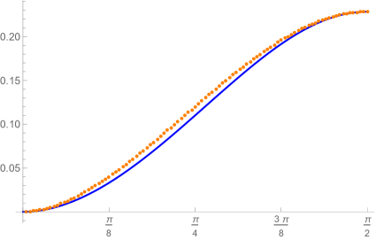
Figure 2: Dots: numerical evaluations of $c_{\rm inc}(\mathsf{A},\mathsf{B})$ as a function of $\alpha$. Continuous line: the analytical lower bound $LB(\alpha)$ in (43).

A good analytical lower bound for $c_{\rm inc}(\mathsf{A},\mathsf{B})$ can be found by fixing a trial state $\rho(\phi)$, considering the bi-observables $\mathsf{M}_{\gamma}$ of (34), and then minimizing the error function $S[\mathsf{A},\mathsf{B}\|\mathsf{M}_{\gamma}](\rho(\phi))$ with respect to $\gamma\in[-1,1]$. Indeed, equation (35) yields the inequality $c_{\rm inc}(\mathsf{A},\mathsf{B})\geq\min_{\gamma\in[-1,1]}S[\mathsf{A},\mathsf{B}\|\mathsf{M}_{\gamma}](\rho(\phi))$ for all $\phi\in[0,2\pi)$. A convenient choice for $\phi$, suggested by the results in the case of two orthogonal components, is to take $\phi\in\{\pi/4\pm\alpha/2,\,5\pi/4\pm\alpha/2\}$, so that the corresponding state $\rho(\phi)$ is any eigenprojection of $\vec{a}\cdot\vec{\sigma}$ or $\vec{b}\cdot\vec{\sigma}$; say we take the eigenprojection $\rho_{e}=\rho(\pi/4-\alpha/2)$ of $\vec{a}\cdot\vec{\sigma}$ with positive eigenvalue. Then, we get

$$c_{\rm inc}(\mathsf{A},\mathsf{B})\geq\min_{\gamma\in[-1,1]}S[\mathsf{A},\mathsf{B}\|\mathsf{M}_{\gamma}](\rho_{e})=:LB(\alpha).$$ (39)

In Appendix B.3, the explicit expression of $S[\mathsf{A},\mathsf{B}\|\mathsf{M}_{\gamma}](\rho_{e})$ is given in (83), its minimum over $\gamma$ is computed and, for $\alpha\neq\pi/2$, it is found at the point

$$\gamma=\frac{\sqrt{2}\ell-a_{2}}{a_{1}},$$ (40)

where

$$\ell=\frac{1}{2\sqrt{2}\,a_{2}}\left(\sqrt{u^{2}+8(1+u)a_{2}^{\,2}}-u\right),$$ (41)

$$u=\left(a_{1}+\frac{1}{\sqrt{2}}\right)\frac{a_{1}^{\,2}-a_{2}^{\,2}}{\sqrt{2}}=\left(1+\sqrt{1+\sin\alpha}\right)\frac{\sin\alpha}{2}\,.$$ (42)

In particular, the value (40) for $\gamma$, together with the fact that the bi-observable $\mathsf{M}_{\gamma}$ has marginals $\mathsf{M}_{\gamma\,[1]}=\mathsf{A}_{\vec{c}(\gamma)}$ and $\mathsf{M}_{\gamma\,[2]}=\mathsf{B}_{\vec{c}(\gamma)}$, show that the marginals of the bi-observable giving the lower bound (39) are not noisy versions of the target observables $\mathsf{A}$ and $\mathsf{B}$; indeed, $\vec{c}(\gamma)\not\propto\vec{a}$ in this case. Finally, the lower bound turns out to be

$$LB(\alpha)=-\log{w}+\frac{1}{2}\left(1+\cos\alpha\right)\log\frac{1+\cos\alpha}{1+\ell}+\frac{1}{2}\left(1-\cos\alpha\right)\log\frac{1-\cos\alpha}{1-\ell}\,,$$ (43)

with

$$w=\frac{1}{2}+\frac{\sqrt{u^{2}+8(1+u)a_{2}^{\,2}}}{4\sqrt{2}\,a_{1}}+\frac{\sin\alpha}{8}\left(\frac{3}{\sqrt{2}\,a_{1}}-1\right).$$ (44)

The plot of $LB(\alpha)$ is the continuous line in Figure 2.

For $\alpha=0$, the target observables are compatible and $c_{\rm inc}(\mathsf{A},\mathsf{B})=0$. For $\alpha\to 0$ the previous formulae give $u=0$, $\ell=1$, $\vec{c}(\gamma)=\vec{a}\equiv\vec{n}$, and one can check that also the lower bound (43) vanishes, as it must be.

For two orthogonal components, i.e. $\alpha=\pi/2$, the expression (43) gives the exact value (32) of the entropic incompatibility degree, and it is not only a lower bound. This value can be computed by going to the limit $\alpha\to\pi/2$ in (43), or directly by Remark 8 in Appendix B.3.

For $\alpha\in(0,\pi/2)$, Figure 2 shows that the analytical lower bound (43) is not so far from the numerical value.

We now compare our optimal approximate joint measurements with other proposals coming from different approaches. Of course, every approximate joint measurement $\mathsf{M}$ that is optimal with respect to some other criterium will have a divergence from the target observables $(\mathsf{A},\mathsf{B})$ larger or equal than $c_{\rm inc}(\mathsf{A},\mathsf{B})$. We stress that the other two proposals we will consider yield optimal bi-observables of the form $\mathsf{M}_{\gamma}$, in which however the parameter $\gamma$ is different from ours.

We have seen that, when $\alpha=\pi/2$, the incompatibility degree of $\mathsf{A}$ and $\mathsf{B}$, as well as their unique optimal approximate joint measurement $\mathsf{M}_{0}$, can be evaluated analytically. In this special case, it turns out that $\mathsf{M}_{0}$ is optimal also with respect to the other criteria we are going to consider in this section. However, as already said, this is not true for general $\alpha$. In order to show it, we fix the angle $\alpha=\pi/4$, and compare the results of the different criteria in Table 1. We also add a $LB$ column summarizing the parameters for the analytical lower bound (39). The rows provide: (1) the parameter $\gamma$ characterizing the measurement $\mathsf{M}_{\gamma}$; (2) the angle characterizing the pure state $\rho(\phi)$ at which $S[\mathsf{A},\mathsf{B}\|\mathsf{M}_{\gamma}]$ is computed, that is the trial angle $\pi/4-\alpha/2$ in the first column, and the angle maximizing $S[\mathsf{A},\mathsf{B}\|\mathsf{M}_{\gamma}](\rho(\phi))$ in the other ones; (3) the value of $S[\mathsf{A},\mathsf{B}\|\mathsf{M}_{\gamma}](\rho(\phi))$ for the parameters chosen in (1) and (2), which gives $LB(\pi/4)$ in the first column and the entropic divergence $D\big{(}\mathsf{A},\mathsf{B}\|\mathsf{M}_{\gamma}\big{)}$ in the other ones.

Table 1: Incompatibility degree and its bounds for $\alpha=\pi/4$.

criterium	$LB$	$c_{\rm inc}$	BLW	NV
measurement: $\gamma\simeq$	0.795559	0.743999	0.541195	0.414213
state: $\phi\simeq$	0.392699	0.282743	0.391128	0.416889
value: $S[\mathsf{A},\mathsf{B}\|\mathsf{M}_{\gamma}](\rho(\phi))\simeq$	0.110081	0.120035	0.160886	0.212079

The description of the columns is as follows.

$LB$: The choice of the parameters is the one described in the computation of the analytical lower bound for $c_{\rm inc}$. The parameter $\gamma$ comes from (40), the angle $\phi=\pi/8$ corresponds to the trial state $\rho_{e}=\rho(\pi/8)$ (i.e. the eigenprojection of $\vec{a}\cdot\vec{\sigma}$ for $\alpha=\pi/4$), and the corresponding value of $S[\mathsf{A},\mathsf{B}\|\mathsf{M}_{\gamma}](\rho_{e})$ is the lower bound $LB(\pi/4)$.

$c_{\rm inc}$: The parameters are chosen following the relative entropy approach to MURs. They are the numerical solution of the minimax problem (35). Thus, the value of $S[\mathsf{A},\mathsf{B}\|\mathsf{M}_{\gamma}](\rho(\phi))$ is the one found numerically for $c_{\rm inc}(\mathsf{A},\mathsf{B})$, i.e. the dot at $\alpha=\pi/4$ in Figure 2; $\gamma$ is the corresponding minimum point giving the optimal approximate joint measurement $\mathsf{M}_{\gamma}$ of $\mathsf{A}$ and $\mathsf{B}$; the angle $\phi$ corresponds to the state at which the error function $S[\mathsf{A},\mathsf{B}\|\mathsf{M}_{\gamma}]$ attains its maximum.

BLW: As discussed in Section 2.3, in [6, 7, 8] a different approach is proposed. In particular, its application to the case of two spin-1/2 components is given in [9] (see also [26], where the same final results are obtained in a slightly different context). There, the authors find a strictly positive lower bound for the sum $d(\mathsf{A},\mathsf{M}_{[1]})^{2}+d(\mathsf{B},\mathsf{M}_{[2]})^{2}$, which holds for all approximate joint measurements $\mathsf{M}$. Moreover, they find a couple of compatible observables $(\mathsf{A}_{\vec{c}},\mathsf{B}_{\vec{c}})$ saturating the lower bound, and thus optimally approximating the target observables $(\mathsf{A},\mathsf{B})$; this couple is given by a vector $\vec{c}$ yielding compatible $\mathsf{A}_{\vec{c}}$ and $\mathsf{B}_{\vec{c}}$, and lying as close as possible to the target direction $\vec{a}$. Referring to Figure 3 in Appendix B.1, this amounts to requiring that $\vec{c}$ is the orthogonal projection of $\vec{a}$ on the right edge of the square $Q$ in the $\vec{i}\vec{j}$-plane; such a square is the region of the plane where the approximating observables $\mathsf{A}_{\vec{c}}$ and $\mathsf{B}_{\vec{c}}$ are compatible (see Proposition 17, item (ii), in Appendix B.1). Using the parametrization $\vec{c}(\gamma)$ given in (33) for the right edge of $Q$, we see that this approach fixes $\gamma=\sqrt{2}a_{2}$. The entropic divergence of the corresponding bi-observable $\mathsf{M}_{\gamma}$ from $(\mathsf{A},\mathsf{B})$ and the angle of the state $\rho(\phi)$ at which it is attained are the content of the BLW column.

NV: At the end of Section 2.4, we briefly discussed the proposal of [45, 49] to use approximating joint measurements whose marginals are noisy versions (NV) of the two target observables. In this approach, one approximates the target observables by means of a compatible couple $(\mathsf{A}_{\vec{c}},\mathsf{B}_{\vec{c}})$ with $\vec{c}\parallel\vec{a}$. Still making reference to Figure 3 in the appendix, the best choice is then picking $\vec{c}$ as large as possible; in this way, $\vec{c}$ lies where the right edge of the compatibility square $Q$ intersects the line joining $\vec{a}$ and the origin. With our parametrization $\vec{c}(\gamma)$ of the edge, this implies $\gamma=a_{2}/a_{1}$. The results for this choice (together with the corresponding maximizing state) are reported in the last column.

3.3 Two conjugate observables in prime power dimension

We now consider two complementary observables in prime power dimension, realized by a couple of MUBs that are conjugated by the Fourier transform of a finite field. In general, the construction of a maximal set of MUBs in a prime power dimensional Hilbert space by using finite fields is well known since Wootters and Fields’ seminal paper [53]; see also [54, Sect. 2] for a review, and [55, 56, 57] for a group theoretic perspective on the topic.

Let $\mathbb{F}$ be a finite field with characteristic $p$. We refer to [58, Sect. V.5] for the basic notions on finite fields. Here we only recall that $p$ is a prime number, and $\mathbb{F}$ has cardinality $|\mathbb{F}|=p^{n}$ for some positive integer $n$. We need also the field trace  ${\rm tr}\,:\mathbb{F}\to{\mathbb{Z}}_{p}$ defined by ${\rm tr}\,{x}=\sum_{k=0}^{n-1}x^{p^{k}}$ (see [58, Sect. VI.5] for its definition and properties).

We consider the Hilbert space $\mathscr{H}=\ell^{2}(\mathbb{F})$, with dimension $d=p^{n}$, and we let our target observables be the two sharp rank-one observables $\mathsf{Q}$ and $\mathsf{P}$ with outcome spaces $\mathscr{X}=\mathscr{Y}=\mathbb{F}$, given by

$$\mathsf{Q}(x)=\left|\,\delta_{x}\,\right\rangle\left\langle\,\delta_{x}\,\right|,\qquad\mathsf{P}(y)=\left|\,\omega_{y}\,\right\rangle\left\langle\,\omega_{y}\,\right|,\qquad\forall x,y\in\mathbb{F}.$$ (45)

In this formula, $\delta_{x}$ is the delta function at $x$, and

$$\omega_{y}(z)=\frac{1}{\sqrt{d}}\,\mathrm{e}^{\frac{2\pi\mathrm{i}}{p}\,{\rm tr}\,yz}\equiv(F^{*}\delta_{y})(z)\quad\text{with}\quad F\phi(z)=\frac{1}{\sqrt{d}}\sum_{t\in\mathbb{F}}\mathrm{e}^{-\frac{2\pi\mathrm{i}}{p}\,{\rm tr}\,zt}\phi(t).$$ (46)

Since $|\left\langle\,\delta_{x}\,|\,\omega_{y}\,\right\rangle|=1/\sqrt{d}$ for all $x$ and $y$, the two orthonormal bases $\{\delta_{x}\}_{x\in\mathbb{F}}$ and $\{\omega_{y}\}_{y\in\mathbb{F}}$ satisfy the MUB condition. In particular, as a consequence of the bound in [17], their preparation uncertainty coefficient (18) is

$$c_{\rm prep}(\mathsf{Q},\mathsf{P})=\log d.$$ (47)

In (46), the operator $F:\mathscr{H}\to\mathscr{H}$ is the unitary discrete Fourier transform over the field $\mathbb{F}$. The observables $\mathsf{Q}$ and $\mathsf{P}$ are then an example of Fourier conjugate MUBs, as $\mathsf{P}(y)=F^{*}\mathsf{Q}(y)F$ for all $y\in\mathbb{F}$.

The definitions (45) and (46) should be compared with the analogous ones for MUBs that are conjugated by means of the Fourier transform over the cyclic ring ${\mathbb{Z}}_{d}$, see e.g. [59]. In the latter case, the Hilbert space is $\mathscr{H}=\ell^{2}({\mathbb{Z}}_{d})$, and the operator $F$ in (46) is replaced by

$$\mathcal{F}\phi(z)=\frac{1}{\sqrt{d}}\sum_{t\in{\mathbb{Z}}}\mathrm{e}^{-\frac{2\pi\mathrm{i}}{d}\,zt}\phi(t)$$ (48)

(cf. [59, Eq. (4)]; note that no field trace appears in this formula). The two definitions are clearly the same if $\mathbb{F}$ coincides with the cyclic field ${\mathbb{Z}}_{p}$ (i.e. $n=1$ and so $d=p$), but they are essentially different in general. Indeed, as observed in [54, Sect. 5.3], they are inequivalent already for $d=2^{2}$.

The following theorem is the main result of this section.

Theorem 13.

For the two sharp observables $\mathsf{Q}$ and $\mathsf{P}$ defined in (45), we have

$$\log\frac{2\sqrt{d}}{\sqrt{d}+1}\leq c_{\rm inc}(\mathsf{Q},\mathsf{P})=\max_{\begin{subarray}{c}\rho\in\mathscr{S}(\mathscr{H})\\ \rho\ \mathrm{pure}\end{subarray}}\left[S\big{(}\mathsf{Q}^{\rho}\|\mathsf{Q}^{\rho}_{\lambda_{0}}\big{)}+S\big{(}\mathsf{P}^{\rho}\|\mathsf{P}^{\rho}_{\lambda_{0}}\big{)}\right]\leq 2\log\frac{2(d+1)}{d+3}\,,$$ (49)

where $\mathsf{Q}_{\lambda_{0}}=\lambda_{0}\mathsf{Q}+(1-\lambda_{0})\mathsf{U}_{\mathbb{F}}$ and $\mathsf{P}_{\lambda_{0}}=\lambda_{0}\mathsf{P}+(1-\lambda_{0})\mathsf{U}_{\mathbb{F}}$ are the uniformly noisy versions of the observables $\mathsf{Q}$ and $\mathsf{P}$ with noise intensity

$$1-\lambda_{0}=\frac{\sqrt{d}}{2(\sqrt{d}+1)}\,.$$ (50)

An optimal approximate joint measurement $\mathsf{M}\in\mathscr{M}_{\rm inc}(\mathsf{A},\mathsf{B})$ is given by

$$\mathsf{M}_{0}(x,y)=\frac{1}{2(d+\sqrt{d})}\left|\,\psi_{x,y}\,\right\rangle\left\langle\,\psi_{x,y}\,\right|\quad\text{with}\quad\psi_{x,y}=\delta_{x}+\mathrm{e}^{-\frac{2\pi\mathrm{i}}{p}\,{\rm tr}\,xy}F\delta_{-y}.$$ (51)

If $p\neq 2$, then $\mathsf{M}_{0}$ is the unique optimal approximate joint measurement of $\mathsf{Q}$ and $\mathsf{P}$, i.e.  $\mathscr{M}_{\rm inc}(\mathsf{Q},\mathsf{P})=\{\mathsf{M}_{0}\}$.

As in the case of the two spin-1/2 components, the proof of this theorem relies on a detailed study of the symmetries of the pair of observables $(\mathsf{Q},\mathsf{P})$, and a subsequent application of Theorem 8. The symmetries and the proof of the theorem are given in Appendix C. Here we briefly comment on its statements and provide a simple example.

Remark 5.

1. Since $\mathsf{Q}$ and $\mathsf{P}$ are sharp, the inequality (49) also gives a bound for the index $c_{\rm ed}(\mathsf{Q},\mathsf{P})=c_{\rm inc}(\mathsf{Q},\mathsf{P})$.

2. The two bounds in (49) are not asymptotically optimal for $d\to\infty$, as the lower bound tends to $1$ while the upper bound goes to $2$.

3. The value in (50) is the minimal noise intensity making the two uniformly noisy observables $\mathsf{Q}_{\lambda_{0}}$ and $\mathsf{P}_{\lambda_{0}}$ compatible [59, Prop. 5 and Ex. 1].

4. In the terminology of [24, 25], the bi-observable in (51) is the covariant phase-space observable generated by the state $[\sqrt{d}/(2\sqrt{d}+2)]\left|\,\psi_{0,0}\,\right\rangle\left\langle\,\psi_{0,0}\,\right|=d\mathsf{M}_{0}(0,0)$ (see (89) and the discussion below it for further details on covariant phase-space observables).

5. Our choice of using the field $\mathbb{F}$ instead of the ring ${\mathbb{Z}}_{d}$ in defining the Fourier operator in (46), and the consequent restriction to only prime power dimensional systems, comes from the fact that the resulting MUBs (45) share dilational symmetries that are not present in the $\mathcal{F}$-conjugate ones. These extra symmetries drastically reduce the number of parameters to be optimized for finding an element of $\mathscr{M}_{\rm inc}(\mathsf{A},\mathsf{B})$ (see Remark 10.2 for further details).

6. The uniqueness property of the optimal approximate joint measurement $\mathsf{M}_{0}$ in odd prime power dimensions should be compared with the measurement uncertainty region for two qudit observables found in [10, Sect. 5.3]. In particular, we remark that there is a whole family of covariant phase-space observables saturating the uncertainty bound of [10, Eq. (38)]. Our optimal bi-observable $\mathsf{M}_{0}$ just corresponds to one of them, that is, the one generated by the state $\rho=d\mathsf{M}_{0}(0,0)$.

7. When $d=2^{n}$ with $n\geq 2$, it is not clear whether or not the set $\mathscr{M}_{\rm inc}(\mathsf{Q},\mathsf{P})$ is made up of a unique bi-observable. However, in the simplest case $d=2$ we have already shown that $\mathscr{M}_{\rm inc}(\mathsf{Q},\mathsf{P})=\{\mathsf{M}_{0}\}$ (see Theorem 11).

Example 1 (Two orthogonal spin-1/2 components).

Let us consider as target observables the two sharp spin-1/2 components $\mathsf{X},\mathsf{Y}\in\mathscr{M}(\{+1,-1\})$ associated with the first two Pauli matrices, defined in (30). This is the easiest example of two Fourier conjugate MUBs. To see this, take the cyclic field $\mathbb{F}={\mathbb{Z}}_{2}\equiv\{0,1\}$, corresponding to the choice $d=p=2$, $n=1$, ${\rm tr}\,x=x$, and identify the observables $\mathsf{Q}(x)=\mathsf{X}\left((-1)^{x}\right)$ and $\mathsf{P}(y)=\mathsf{Y}\left((-1)^{y}\right)$ ($x,y=0,1$) by setting $\sigma_{1}=|\delta_{0}\rangle\langle\delta_{0}|-|\delta_{1}\rangle\langle\delta_{1}|$, and $\sigma_{2}=|\delta_{0}\rangle\langle\delta_{1}|+|\delta_{1}\rangle\langle\delta_{1}|$. With this identification, the discrete Fourier transform becomes $F=\left(\sigma_{1}+\sigma_{2}\right)/\sqrt{2}\equiv\mathrm{i}\exp\{-\mathrm{i}\pi\vec{n}\cdot\vec{\sigma}/2\}$. We have already found in (31) the optimal joint observable of $\mathsf{X}$ and $\mathsf{Y}$, together with the value of the entropic incompatibility degree. These are precisely the bi-observable and the lower bound found in Theorem 13.

4 Entropic measurement uncertainty relations for $n$ observables

Uncertainty relations have been studied also in the case of more than two observables, see e.g. [13, 22, 19] for the case of entropic PURs. Both our entropic coefficients (10) and (12) (and the related MURs) can be generalized to the case of $n>2$ target observables. However, in the case of $c_{\rm ed}(\mathsf{A}_{1},\ldots,\mathsf{A}_{n})$ an order of observation has to be fixed, and one needs to point out the subset of the observables for which imprecise measurements are allowed (the analogues of the observable $\mathsf{A}$ in the binary case of $c_{\rm ed}(\mathsf{A},\mathsf{B})$) from those observables that are kept fixed and get disturbed by the other measurements (similar to $\mathsf{B}$ in $c_{\rm ed}(\mathsf{A},\mathsf{B})$). Thus, different definitions of $c_{\rm ed}$ are possible in the $n$-observable case. This leads us to generalize only the entropic incompatibility degree $c_{\rm inc}(\mathsf{A}_{1},\ldots,\mathsf{A}_{n})$, whose definition is straightforward and gives a lower bound for $c_{\rm ed}$, independently of its possible definitions.

4.1 Entropic incompatibility degree and MURs

Let $\mathsf{A}_{1},\ldots,\mathsf{A}_{n}$ be $n$ fixed observables with outcome sets $\mathscr{X}_{1},\ldots,\mathscr{X}_{n}$, respectively. As usual, we assume that all the sets $\mathscr{X}_{i}$ are finite. The observables with outcomes in the product set $\mathscr{X}_{1\cdots n}=\mathscr{X}_{1}\times\cdots\times\mathscr{X}_{n}$ are called multi-observables, and we use the notation $\mathscr{M}(\mathscr{X}_{1\cdots n})$ for the set of all such observables. If $\mathsf{M}\in\mathscr{M}(\mathscr{X}_{1\cdots n})$, its $i$-th marginal observable is the element $\mathsf{M}_{[i]}\in\mathscr{M}(\mathscr{X}_{i})$, with

$$\mathsf{M}_{[i]}(x)=\sum_{x_{j}\in\mathscr{X}_{j}:j\neq i}\mathsf{M}(x_{1},\ldots,x_{i-1},x,x_{i+1},\ldots,x_{n}).$$

The notion of compatibility straightforwardly extends to the case of $n$ observables.

As in the $n=2$ case, we regard any $\mathsf{M}\in\mathscr{M}(\mathscr{X}_{1\cdots n})$ as an approximate joint measurement of $\mathsf{A}_{1},\ldots$, $\mathsf{A}_{n}$. For all $\rho\in\mathscr{S}(\mathscr{H})$, the total amount of information loss in the distribution approximations $\mathsf{A}_{i}^{\rho}\simeq\mathsf{M}_{[i]}^{\rho}$, $i=1,\ldots,n$, is the sum of the respective relative entropies. Then, we have the following generalization of Definitions 1, 2 and 3.

Definition 5.

For any multi-observable  $\mathsf{M}\in\mathscr{M}(\mathscr{X}_{1\cdots n})$,  the error function of the approximation
$(\mathsf{A}_{1},\ldots,\mathsf{A}_{n})\simeq(\mathsf{M}_{[1]},\ldots,\mathsf{M}_{[n]})$ is the state-dependent quantity

$$S[\mathsf{A}_{1},\ldots,\mathsf{A}_{n}\|\mathsf{M}](\rho)=\sum_{i=1}^{n}S\big{(}\mathsf{A}^{\rho}_{i}\|\mathsf{M}^{\rho}_{[i]}\big{)}.$$ (52)

The entropic divergence of $\mathsf{M}\in\mathscr{M}(\mathscr{X}_{1\cdots n})$ from $(\mathsf{A}_{1},\ldots,\mathsf{A}_{n})$ is

$$D\big{(}\mathsf{A}_{1},\ldots,\mathsf{A}_{n}\|\mathsf{M}\big{)}=\sup_{\rho\in\mathscr{S}(\mathscr{H})}S[\mathsf{A}_{1},\ldots,\mathsf{A}_{n}\|\mathsf{M}](\rho).$$ (53)

The entropic incompatibility degree of the observables $\mathsf{A}_{1},\ldots,\mathsf{A}_{n}$ is

$$c_{\rm inc}\big{(}\mathsf{A}_{1},\ldots,\mathsf{A}_{n}\big{)}=\inf_{\mathsf{M}\in\mathscr{M}(\mathscr{X}_{1\cdots n})}D\big{(}\mathsf{A}_{1},\ldots,\mathsf{A}_{n}\|\mathsf{M}\big{)}.$$ (54)

We still denote by

$$\mathscr{M}_{\rm inc}(\mathsf{A}_{1},\ldots,\mathsf{A}_{n})=\operatornamewithlimits{arg\,min}_{\mathsf{M}\in\mathscr{M}(\mathscr{X}_{1\cdots n})}D\big{(}\mathsf{A}_{1},\ldots,\mathsf{A}_{n}\|\mathsf{M}\big{)}$$

the set of the optimal approximate joint measurements of $\mathsf{A}_{1},\ldots,\mathsf{A}_{n}$. As in the case with $n=2$, the optimality of a multi-observable $\mathsf{M}$ depends only on its marginals $\mathsf{M}_{[i]}$, since the entropic divergence itself depends only on such marginals.

We have the following extension of Theorems 3, 6 and 7.

Theorem 14.

Let $\mathsf{A}_{i}\in\mathscr{M}(\mathscr{X}_{i})$, $i=1,\ldots,n$, be the target observables. The error function, entropic divergence and incompatibility degree satisfy the following properties.

1. The function $S[\mathsf{A}_{1},\ldots,\mathsf{A}_{n}\|\mathsf{M}]:\mathscr{S}(\mathscr{H})\to[0,+\infty]$ is convex and LSC, $\forall\mathsf{M}\in\mathscr{M}(\mathscr{X}_{1\cdots n})$.

2. The function $D\big{(}\mathsf{A}_{1},\ldots,\mathsf{A}_{n}\|\cdot\big{)}:\mathscr{M}(\mathscr{X}_{1\cdots n})\to[0,+\infty]$ is convex and LSC.

3. For any $\mathsf{M}\in\mathscr{M}(\mathscr{X}_{1\cdots n})$, the following three statements are equivalent:

   1. $D\big{(}\mathsf{A}_{1},\ldots,\mathsf{A}_{n}\|\mathsf{M}\big{)}<+\infty$,

   2. $\operatorname{ker}\mathsf{M}_{[i]}(x)\subseteq\operatorname{ker}\mathsf{A}_{i}(x)\quad\forall x,\ \forall i$,

   3. $S[\mathsf{A}_{1},\ldots,\mathsf{A}_{n}\|\mathsf{M}]$ is bounded and continuous.

4. $\displaystyle D\big{(}\mathsf{A}_{1},\ldots,\mathsf{A}_{n}\|\mathsf{M}\big{)}=\max_{\rho\in\mathscr{S}(\mathscr{H}),\ \rho\ \mathrm{pure}}S[\mathsf{A}_{1},\ldots,\mathsf{A}_{n}\|\mathsf{M}](\rho)$, where the maximum can be any value in the extended interval $[0,+\infty]$.

5. The quantities $S[\mathsf{A},\mathsf{B}\|\mathsf{M}](\rho)$, $D\big{(}\mathsf{A}_{1},\ldots,\mathsf{A}_{n}\|\mathsf{M}\big{)}$ and $c_{\rm inc}(\mathsf{A}_{1},\ldots,\mathsf{A}_{n})$ are invariant under an overall unitary conjugation of the state $\rho$ and the observables $\mathsf{A}_{1},\ldots,\mathsf{A}_{n}$ and $\mathsf{M}$, and they do not depend on the labelling of the outcomes in $\mathscr{X}_{1},\ldots,\mathscr{X}_{n}$.

6. $c_{\rm inc}(\mathsf{A}_{\sigma(1)},\ldots,\mathsf{A}_{\sigma(n)})=c_{\rm inc}(\mathsf{A}_{1},\ldots,\mathsf{A}_{n})$ for any permutation $\sigma$ of the index set $\{1,\ldots,n\}$.

7. The entropic incompatibility coefficient $c_{\rm inc}(\mathsf{A}_{1},\ldots,\mathsf{A}_{n})$ is always finite, and it satisfies the bounds

   $$c_{\rm inc}(\mathsf{A}_{1},\ldots,\mathsf{A}_{n})\leq\sum_{i=1}^{n}\log|\mathscr{X}_{i}|-\inf_{\rho\in\mathscr{S}(\mathscr{H})}\sum_{i=1}^{n}H(\mathsf{A}_{i}^{\rho}),$$ (55)

   $$c_{\rm inc}(\mathsf{A}_{1},\ldots,\mathsf{A}_{n})\leq\sum_{i=1}^{n}\log\frac{n(d+1)}{d+n+(n-1)\min_{x\in\mathscr{X}_{i}}{\rm Tr}\,\{\mathsf{A}_{i}(x)\}}\\ {}\leq n\log\frac{n(d+1)}{d+n}\leq n\log n.$$ (56)

8. The set $\mathscr{M}_{\rm inc}(\mathsf{A}_{1},\ldots,\mathsf{A}_{n})$ is a nonempty convex compact subset of $\mathscr{M}(\mathscr{X}_{1\cdots n})$.

9. $c_{\rm inc}(\mathsf{A}_{1},\ldots,\mathsf{A}_{n})=0$ if and only if the observables $\mathsf{A}_{1},\ldots,\mathsf{A}_{n}$ are compatible, and in this case $\mathscr{M}_{\rm inc}(\mathsf{A}_{1},\ldots,\mathsf{A}_{n})$ is the set of all the joint measurements of $\mathsf{A}_{1},\ldots,\mathsf{A}_{n}$.

10. If $\mathsf{A}_{n+1}\in\mathscr{M}(\mathscr{X}_{n+1})$ is another observable, then we have $c_{\rm inc}(\mathsf{A}_{1},\ldots,\mathsf{A}_{n+1})\geq c_{\rm inc}(\mathsf{A}_{1},\ldots,\mathsf{A}_{n})$.

Proof.

The proofs of items (i)–(vi), (viii) and (ix) are straightforward extensions of the analogous ones for two observables.

In item (vii), the upper bound (55) follows by evaluating the entropic divergence of the uniform observable $\mathsf{U}=(u_{\mathscr{X}_{1}}\otimes\cdots\otimes u_{\mathscr{X}_{n}})\,{\mathbbm{1}}$ from $(\mathsf{A}_{1},\ldots,\mathsf{A}_{n})$:

$$c_{\rm inc}(\mathsf{A}_{1},\ldots,\mathsf{A}_{n}) \leq D\big{(}\mathsf{A}_{1},\ldots,\mathsf{A}_{n}\|\mathsf{U}\big{)}=\sup_{\rho\in\mathscr{S}(\mathscr{H})}\sum_{i=1}^{n}S\big{(}\mathsf{A}^{\rho}_{i}\|u_{\mathscr{X}_{i}}\big{)}$$

$$=\sup_{\rho\in\mathscr{S}(\mathscr{H})}\sum_{i=1}^{n}\left[\log|\mathscr{X}_{i}|-H(\mathsf{A}^{\rho}_{i})\right]\qquad\text{by Proposition \ref{prop:propHSrel}, item (\ref{HSrel});}$$

this yields (55).

The upper bound (56) follows by using an approximate cloning argument, just as in the case of only two observables. Indeed, the optimal approximate $n$-cloning channel is the map

$$\Phi:\mathscr{S}(\mathscr{H})\to\mathcal{S}(\mathscr{H}^{\otimes n}),\qquad\Phi(\rho)=\frac{d!n!}{(d+n-1)!}S_{n}(\rho\otimes{\mathbbm{1}}^{\otimes(n-1)})S_{n},$$

where $S_{n}$ is the orthogonal projection of $\mathscr{H}^{\otimes n}$ onto its symmetric subspace ${\rm Sym}(\mathscr{H}^{\otimes n})$ [50]. Evaluating the marginals of the multi-observable $\mathsf{M}_{\rm cl}=\Phi^{*}(\mathsf{A}_{1}\otimes\cdots\otimes\mathsf{A}_{n})$, we obtain the noisy versions

$$\mathsf{M}_{{\rm cl}\,[i]}=\mathsf{A}_{i\,\lambda_{\rm cl}},\qquad\text{where}\qquad\lambda_{\rm cl}=\frac{d+n}{n(d+1)}$$

(see [51]). Since $c_{\rm inc}(\mathsf{A}_{1},\ldots,\mathsf{A}_{n})\leq D\big{(}\mathsf{A}_{1},\ldots,\mathsf{A}_{n}\|\mathsf{M}_{\rm cl}\big{)}$, a computation similar to the one for obtaining the bound (17) in Section 2.4 then yields the bounds (56).

Finally, in order to prove item (x), take any $\mathsf{M}^{\prime}\in\mathscr{M}(\mathscr{X}_{1}\times\cdots\times\mathscr{X}_{n+1})$, and let

$$\mathsf{M}(x_{1},\ldots,x_{n})=\sum_{x\in\mathscr{X}_{n+1}}\mathsf{M}^{\prime}(x_{1},\ldots,x_{n},x).$$

We have $\mathsf{M}^{\prime}_{[i]}=\mathsf{M}_{[i]}$ for all $i=1,\ldots,n$, hence

$$c_{\rm inc}(\mathsf{A}_{1},\ldots,\mathsf{A}_{n})\leq D\big{(}\mathsf{A}_{1},\ldots,\mathsf{A}_{n}\|\mathsf{M}\big{)}=\sup_{\rho}\sum_{i=1}^{n}S\big{(}\mathsf{A}_{i}^{\rho}\|\mathsf{M}^{\rho}_{[i]}\big{)}\\ {}\leq\sup_{\rho}\sum_{i=1}^{n+1}S\big{(}\mathsf{A}_{i}^{\rho}\|\mathsf{M}^{\prime\rho}_{[i]}\big{)}=D\big{(}\mathsf{A}_{1},\ldots,\mathsf{A}_{n+1}\|\mathsf{M}^{\prime}\big{)}.$$

Item (x) then follows by taking the infimum over $\mathsf{M}^{\prime}$. ∎

The monotonicity property (x), which is specific of the many observable case, is another desirable feature for an incompatibility coefficient: the amount of incompatibility cannot decrease when an extra observable is added.

Remark 6 (MURs).

Theorem 14 gives the following extension of the entropic MURs (13) and (14):

$$D\big{(}\mathsf{A}_{1},\ldots,\mathsf{A}_{n}\|\mathsf{M}\big{)}\geq c_{\rm inc}(\mathsf{A}_{1},\ldots,\mathsf{A}_{n}),\qquad\forall\mathsf{M}\in\mathscr{M}(\mathscr{X}_{1\cdots n}),$$ (57)

$$\forall\mathsf{M}\in\mathscr{M}(\mathscr{X}_{1\cdots n}),\ \ \exists\rho\in\mathscr{S}(\mathscr{H}):\ \ \sum_{i=1}^{n}S\big{(}\mathsf{A}_{i}^{\rho}\|\mathsf{M}^{\rho}_{[i]}\big{)}\geq c_{\rm inc}(\mathsf{A}_{1},\ldots,\mathsf{A}_{n}).$$ (58)

Finally, suppose the product space $\mathscr{X}_{1\cdots n}$ carries the action of a finite symmetry group $G$, which also acts on the quantum system Hilbert space $\mathscr{H}$ by means of a projective unitary representation $U$. These actions then extend to the set of states $\mathscr{S}(\mathscr{H})$, the set of probabilities $\mathscr{P}(\mathscr{X}_{1\cdots n})$ and the set of multi-observables $\mathscr{M}(\mathscr{X}_{1\cdots n})$ exactly as in Section 3.1. Similarly, for any $\mathsf{M}\in\mathscr{M}(\mathscr{X}_{1\cdots n})$, we can define its covariant version $\mathsf{M}_{G}$. Then, the content of Theorem 8 and Corollary 9 can be translated to the case of $n$ observables as follows.

Theorem 15.

Let $\mathsf{A}_{i}\in\mathscr{M}(\mathscr{X}_{i})$, $i=1,\ldots,n$, be the target observables. Suppose the finite group $G$ acts on both the output space $\mathscr{X}_{1\cdots n}$ and the index set $\{1,\ldots,n\}$, and it also acts with a projective unitary representation $U$ on $\mathscr{H}$. Moreover, assume that $G$ is generated by a subset $S_{G}\subseteq G$ such that, for every $g\in S_{G}$ and $i\in\{1,\ldots,n\}$, there exists a bijective map $f_{g,i}:\mathscr{X}_{i}\to\mathscr{X}_{gi}$ for which

1. $g(x_{1},\ldots,x_{n})_{gi}=f_{g,i}(x_{i})$ for all $(x_{1},\ldots,x_{n})\in\mathscr{X}_{1\cdots n}$,

2. $U_{g}\mathsf{A}_{i}(x_{i})U_{g}^{*}=\mathsf{A}_{gi}(f_{g,i}(x_{i}))$ for all $x_{i}\in\mathscr{X}_{i}$.

Then,

1. $D\big{(}\mathsf{A}_{1},\ldots,\mathsf{A}_{n}\|g\mathsf{M}\big{)}=D\big{(}\mathsf{A}_{1},\ldots,\mathsf{A}_{n}\|\mathsf{M}\big{)}$ for all $\mathsf{M}\in\mathscr{M}(\mathscr{X}_{1\cdots n})$ and $g\in G$;

2. the set $\mathscr{M}_{\rm inc}(\mathsf{A}_{1},\ldots,\mathsf{A}_{n})$ is $G$-invariant;

3. for any $\mathsf{M}\in\mathscr{M}_{\rm inc}(\mathsf{A}_{1},\ldots,\mathsf{A}_{n})$, we have $\mathsf{M}_{G}\in\mathscr{M}_{\rm inc}(\mathsf{A}_{1},\ldots,\mathsf{A}_{n})$;

4. there exists a $G$-covariant observable in $\mathscr{M}_{\rm inc}(\mathsf{A}_{1},\ldots,\mathsf{A}_{n})$.

Proof.

As in the proof of Theorem 8, it is not restrictive to assume that $S_{G}=G$. For all $p\in\mathscr{P}(\mathscr{X}_{1\cdots n})$, condition (a) implies

$$gp_{[i]}(x_{i}) =\sum_{\begin{subarray}{c}x_{j}\in\mathscr{X}_{j}\\ \text{s.t.\leavevmode\nobreak\ }j\neq i\end{subarray}}gp(x_{1},\ldots,x_{n})=\sum_{\begin{subarray}{c}x_{gj}\in\mathscr{X}_{gj}\\ \text{s.t.\leavevmode\nobreak\ }gj\neq i\end{subarray}}p(f_{g^{-1},g1}(x_{g1}),\ldots,f_{g^{-1},gn}(x_{gn}))$$

$$=\sum_{\begin{subarray}{c}y_{j}\in\mathscr{X}_{j}\\ \text{s.t.\leavevmode\nobreak\ }gj\neq i\end{subarray}}p(y_{1},\ldots,y_{n})\qquad\qquad\text{where $y_{j}=f_{g^{-1},gj}(x_{gj})$}$$

$$=\sum_{\begin{subarray}{c}y_{j}\in\mathscr{X}_{j}\\ \text{s.t.\leavevmode\nobreak\ }j\neq g^{-1}i\end{subarray}}p(y_{1},\ldots,y_{n})=p_{[g^{-1}i]}(y_{g^{-1}i})$$

$$=p_{[g^{-1}i]}(f_{g^{-1},i}(x_{i})),$$

and hence

$$(gp_{[1]}\otimes\cdots\otimes gp_{[n]})(x_{1},\ldots,x_{n})=\prod_{i=1}^{n}gp_{[i]}(x_{i})=\prod_{i=1}^{n}p_{[g^{-1}i]}(f_{g^{-1},i}(x_{i}))\\ {}=\prod_{i=1}^{n}p_{[i]}(f_{g^{-1},gi}(x_{gi}))=g(p_{[1]}\otimes\cdots\otimes p_{[n]})(x_{1},\ldots,x_{n}).$$

Therefore,

$$gp_{[1]}\otimes\cdots\otimes gp_{[n]}=g(p_{[1]}\otimes\cdots\otimes p_{[n]}).$$ (59)

On the other hand, by condition (b) we have $\mathsf{A}^{g\rho}_{i}(x_{i})=\mathsf{A}^{\rho}_{g^{-1}i}(f_{g^{-1},i}(x_{i}))$, and then

$$(\mathsf{A}_{1}^{g\rho}\otimes\cdots\otimes\mathsf{A}_{n}^{g\rho})(x_{1},\ldots,x_{n})=\prod_{i=1}^{n}\mathsf{A}^{\rho}_{g^{-1}i}(f_{g^{-1},i}(x_{i}))=\prod_{i=1}^{n}\mathsf{A}^{\rho}_{i}(f_{g^{-1},gi}(x_{gi}))$$

$$\qquad\qquad\qquad\qquad=g(\mathsf{A}_{1}^{\rho}\otimes\cdots\otimes\mathsf{A}_{n}^{\rho})(x_{1},\ldots,x_{n}),$$

that is,

$$\mathsf{A}_{1}^{g\rho}\otimes\cdots\otimes\mathsf{A}_{n}^{g\rho}=g(\mathsf{A}_{1}^{\rho}\otimes\cdots\otimes\mathsf{A}_{n}^{\rho}).$$ (60)

Having established (59) and (60), the proof of the equality $D\big{(}\mathsf{A}_{1},\ldots,\mathsf{A}_{n}\|g\mathsf{M}\big{)}=D\big{(}\mathsf{A}_{1},\ldots,\mathsf{A}_{n}\|\mathsf{M}\big{)}$ follows along the same lines of the proof of Theorem 8. The remaining statements are then proved as in Corollary 9. ∎

In the next section we will use Theorem 15 to solve the case of $n=3$ orthogonal target spin-1/2 components. This is the basic example of a maximal set of $d+1$ MUBs in a $d$-dimensional Hilbert space. It is an open problem whether similar arguments lead to find the incompatibility index $c_{\rm inc}(\mathsf{Q}_{1},\ldots,\mathsf{Q}_{d+1})$ of a maximal set of $d+1$ MUBs $\mathsf{Q}_{1},\ldots,\mathsf{Q}_{d+1}$ whenever such a set of MUBs is known to exist, that is, for all prime powers $d$.

4.2 Three orthogonal spin-1/2 components

Let the target observables $\mathsf{A}_{1}$, $\mathsf{A}_{2}$, $\mathsf{A}_{3}$ be three mutually orthogonal spin-1/2 components, that is, the sharp observables $\mathsf{X}$, $\mathsf{Y}$, $\mathsf{Z}\in\mathscr{M}(\{+1,-1\})$ associated with the three Pauli matrices; the observables $\mathsf{X},\mathsf{Y}$ are given in (30), and

$$\mathsf{Z}(z)=\frac{1}{2}\left({\mathbbm{1}}+z\sigma_{3}\right),\qquad\forall z\in\mathscr{Z}=\{+1,-1\}.$$ (61)

Then, we have the following three-spin version of Theorem 11.

Theorem 16.

Let $\mathsf{X}$, $\mathsf{Y}$ and $\mathsf{Z}$ be the three orthogonal spin-1/2 components (30), (61). Then, for the following two tri-observables $\mathsf{M}_{0},\mathsf{M}_{1}\in\mathscr{M}(\mathscr{X}\times\mathscr{Y}\times\mathscr{Z})$

$$\mathsf{M}_{0}(x,y,z)=\frac{1}{8}\left[{\mathbbm{1}}+\frac{1}{\sqrt{3}}(x\sigma_{1}+y\sigma_{2}+z\sigma_{3})\right],$$ (62)

$$\begin{gathered}\mathsf{M}_{1}(1,1,-1)=2\mathsf{M}_{0}(1,1,-1),\quad\mathsf{M}_{1}(1,-1,1)=2\mathsf{M}_{0}(1,-1,1),\\ \mathsf{M}_{1}(-1,1,1)=2\mathsf{M}_{0}(-1,1,1),\quad\mathsf{M}_{1}(-1,-1,-1)=2\mathsf{M}_{0}(-1,-1,-1),\\ \mathsf{M}_{1}(x,y,z)=0\quad\text{ otherwise,}\end{gathered}$$ (66)

we have $\mathsf{M}_{0},\mathsf{M}_{1}\in\mathscr{M}_{\rm inc}(\mathsf{X},\mathsf{Y},\mathsf{Z})$. If $\rho_{e}$ is the projection on any eigenvector of $\sigma_{1}$, $\sigma_{2}$ or $\sigma_{3}$, then, for $i=0,1$,

$$c_{\rm inc}(\mathsf{X},\mathsf{Y},\mathsf{Z})=S[\mathsf{X},\mathsf{Y},\mathsf{Z}\|\mathsf{M}_{i}](\rho_{e})=\log\left(3-\sqrt{3}\right)\simeq 0.342497\,.$$ (67)

The description of the symmetry group of $\mathsf{X}$, $\mathsf{Y}$ and $\mathsf{Z}$, and the consequent application of Theorem 15 yielding the proof of Theorem 16, are provided in Appendix B.4.

Note that, differently from the case with only $n=2$ spins, for $n=3$ orthogonal spin-1/2 components there is not a unique optimal approximate joint measurement. It should be also remarked that, although $\mathsf{M}_{0}\neq\mathsf{M}_{1}$, both optimal approximate joint measurements given in (62), (66) have the same marginals, so that $S[\mathsf{X},\mathsf{Y},\mathsf{Z}\|\mathsf{M}_{0}]=S[\mathsf{X},\mathsf{Y},\mathsf{Z}\|\mathsf{M}_{1}]$. Indeed, they are the equally noisy observbles

$$\mathsf{M}_{0[1]}=\mathsf{M}_{1[1]}=\mathsf{X}_{\frac{1}{\sqrt{3}}},\qquad\mathsf{M}_{0[2]}=\mathsf{M}_{1[2]}=\mathsf{Y}_{\frac{1}{\sqrt{3}}},\qquad\mathsf{M}_{0[3]}=\mathsf{M}_{1[3]}=\mathsf{Z}_{\frac{1}{\sqrt{3}}}.$$ (68)

The construction of the tri-observable $\mathsf{M}_{1}$ is taken from [60, Sect. VI]. It is an open question whether $\left(\mathsf{X}_{1/\sqrt{3}},\mathsf{Y}_{1/\sqrt{3}},\mathsf{Z}_{1/\sqrt{3}}\right)$ is the unique triple of compatible observables optimally approximating $(\mathsf{X},\mathsf{Y},\mathsf{Z})$; see also Remark 9 in Appendix B.4 for further comments.

5 Conclusions

We have formulated and proved entropic MURs for discrete observables in a finite-dimensional Hilbert space. In doing so, we have considered target observables $\mathsf{A}$ and $\mathsf{B}$ described by general POVMs, not only sharp observables. Our formulation employs the relative entropy to quantify the total amount of information that is lost when $\mathsf{A}$ and $\mathsf{B}$ are approximated with the marginals $\mathsf{M}_{[1]}$ and $\mathsf{M}_{[2]}$ of a bi-observable $\mathsf{M}$. Such an information loss is the state-dependent error (8); maximizing it over all states $\rho$ and then minimizing the result over the bi-observables $\mathsf{M}$, we have derived our MURs (14): for every approximating bi-observable $\mathsf{M}$, there is always a state $\rho$ such that the total information loss of the approximation $(\mathsf{A}^{\rho},\mathsf{B}^{\rho})\simeq(\mathsf{M}^{\rho}_{[1]},\mathsf{M}^{\rho}_{[2]})$ is not less than a minimal threshold $c(\mathsf{A},\mathsf{B})$, independent of $\mathsf{M}$ and strictly positive when the target observables are incompatible.

Minimizing over different sets of bi-observables yields MURs with different meanings. If $\mathsf{M}$ varies over all the POVMs on the product set of the $\mathsf{A}$- and $\mathsf{B}$-outcomes, then the resulting index $c_{\rm inc}(\mathsf{A},\mathsf{B})$ is the minimal error potentially affecting all possible approximate joint measurements of $\mathsf{A}$ and $\mathsf{B}$. On the other hand, if $\mathsf{M}$ is only allowed to vary over the subset of all the sequential measurements of an approximation of $\mathsf{A}$ followed by $\mathsf{B}$, we obtain the minimal information loss $c_{\rm ed}(\mathsf{A},\mathsf{B})$ due to the error/disturbance tradeoff. We have proved that the two indexes remarkably coincide when the second observable $\mathsf{B}$ is sharp; we have also given explicit examples, involving general POVMs, where the two indexes actually differ.

The two coefficients $c_{\rm inc}$ and $c_{\rm ed}$ play a double role: on the one side, they are the lower bounds of our entropic MURs, as just described above; on the other side, they also properly quantify the degree of (total or sequential) incompatibility of the target observables. The latter interpretation is justified since $c_{\rm inc}$ and $c_{\rm ed}$ only depend on $\mathsf{A}$ and $\mathsf{B}$, as well as by the remarkable properties of the two indexes (Theorem 6). In particular, the existence of an index allows to establish whether a couple of observables is more or less incompatible than another one. For instance, the incompatibility degree of two spin-1/2 components grows by increasing the angle between their directions, as naturally expected (see Figure 2).

Due to the double optimization in the definitions of $c_{\rm inc}(\mathsf{A},\mathsf{B})$ and $c_{\rm ed}(\mathsf{A},\mathsf{B})$, it is not easy to explicitly compute them and their corresponding optimal approximate joint measurements. Anyway, in Theorem 8 we have shown how one can use general symmetry arguments in order to simplify the problem. We have then applied this method to two spin-1/2 components (Theorems 11 and 12), and two Fourier conjugate MUBs in prime power dimension (Theorem 13).

A peculiar feature of our MURs is that in several cases there is actually a unique optimal approximate joint measurement. Indeed, in the two spin and MUB examples, we have uniqueness for all the cases in which we have managed to completely characterize the sets $\mathscr{M}_{\rm inc}$ and $\mathscr{M}_{\rm ed}$ of the optimally approximating joint measurements. We conjecture that this is still true also for the two nonorthogonal spin-1/2 components, and the Fourier conjugated MUBs in even prime power dimensions, for which up to now we have only partial results.

One nice aspect of our approach is that it naturally and easily generalizes to more than two observables. We have done this extension only for the entropic incompatibility degree $c_{\rm inc}$ (Theorems 14 and 15), as the multi-observable interpretation of $c_{\rm ed}$ is less transparent. As an application, we have computed the index $c_{\rm inc}$ for three orthogonal spin-1/2 components $\mathsf{X}$, $\mathsf{Y}$ and $\mathsf{Z}$; although in this case there is still a unique covariant approximate joint measurement, the main difference with the two spin case is that $\mathscr{M}_{\rm inc}(\mathsf{X},\mathsf{Y},\mathsf{Z})$ is not a singleton set now.

Many problems still remain open, as it is not clear how to analytically or at least numerically compute $c_{\rm inc}$ and $c_{\rm ed}$ and the corresponding optimal approximate joint measurements for an arbitrary couple of target observables. Explicit results would be desirable for physically relevant observables other than those considered in Sections 3.2, 3.3 and 4.2 (e.g. two or more spin-$s$ components with $s>1/2$, two or more MUBs in arbitrary dimensions and possibly not Fourier conjugate, etc.). A possible generalization is to include also systems in presence of “quantum memories”; indeed, this extension has recently been studied in the case of entropic PURs [61, 62, 22]. More importantly, the theory we have developed is restricted to discrete observables in a finite-dimensional Hilbert space. The bound $c_{\rm inc}(\mathsf{A}_{1},\ldots,\mathsf{A}_{n})\leq n\log n$ appearing in (17) and (56), which is independent of the number of the outcomes and the dimension of $\mathscr{H}$, suggests that it would be possible to generalize the theory to arbitrary observables in a separable Hilbert space. However, this is not a straightforward extension; indeed, the first results on position and momentum [34] already show that the error function (7) needs to be restricted to only particular classes of states, in order to avoid $c_{\rm inc}=+\infty$, merely due to classical effects.

Appendix A Examples of compatible but not sequentially compatible observables

First example from [27]

Apart from an exchange of $\mathsf{A}$ and $\mathsf{B}$ and some explicit computations, this example is taken from [27, Sect. III.C, and the end of Sect. III.A]. With $\mathscr{H}={\mathbb{C}}^{3}$, $\mathscr{X}=\{1,2\}$ and $\mathscr{Y}=\{1,\ldots,5\}$, the two target observables are defined by

$$\mathsf{A}(1)=\frac{1}{2}\begin{pmatrix}2&0&0\\ 0&0&0\\ 0&0&1\end{pmatrix},\qquad\mathsf{A}(2)=\frac{1}{2}\begin{pmatrix}0&0&0\\ 0&2&0\\ 0&0&1\end{pmatrix};$$

$$\mathsf{B}(1)=\frac{1}{4}\begin{pmatrix}2&0&-\sqrt{2}\\ 0&0&0\\ -\sqrt{2}&0&1\end{pmatrix},\quad\mathsf{B}(2)=\frac{1}{10}\begin{pmatrix}0&0&0\\ 0&1&-2\\ 0&-2&4\end{pmatrix},\quad\mathsf{B}(3)=\frac{1}{2}\begin{pmatrix}0&0&0\\ 0&1&0\\ 0&0&0\end{pmatrix},$$

$$\mathsf{B}(4)=\frac{1}{10}\begin{pmatrix}0&0&0\\ 0&4&2\\ 0&2&1\end{pmatrix},\qquad\mathsf{B}(5)=\frac{1}{4}\begin{pmatrix}2&0&\sqrt{2}\\ 0&0&0\\ \sqrt{2}&0&1\end{pmatrix}.$$

These two observables are compatible, and one can check that a joint observable is

$$\mathsf{M}(1,1)=\mathsf{B}(1),\quad\mathsf{M}(1,5)=\mathsf{B}(5),\quad\mathsf{M}(2,2)=\mathsf{B}(2),\quad\mathsf{M}(2,3)=\mathsf{B}(3),$$

$$\mathsf{M}(2,4)=\mathsf{B}(4),\\ \qquad\mathsf{M}(1,2)=\mathsf{M}(1,3)=\mathsf{M}(1,4)=\mathsf{M}(2,1)=\mathsf{M}(2,5)=0.$$

This implies $c_{\rm inc}(\mathsf{A},\mathsf{B})=0$. Moreover, in [27, Sect. III.C] it is proved that: (1) there exists an instrument implementing $\mathsf{B}$ which does not disturb $\mathsf{A}$; (2) any instrument implementing $\mathsf{A}$ disturbs $\mathsf{B}$. By Theorem 6, item (vi), this implies $c_{\rm ed}(\mathsf{B},\mathsf{A})=0$ and $c_{\rm ed}(\mathsf{A},\mathsf{B})>0$.

Second example from [27]

This is the first example of [27, Sect. III.A], which we report in the particular case in which the noise parameters are fixed and equal; let us call them $\lambda$, with $\lambda\in\left(\frac{1}{2}\,,\,\frac{2}{3}\right]$. The observables are two-valued $(\mathscr{X}=\mathscr{Y}=\{1,2\})$, and they are built up by using two noncommuting orthogonal projections $P$ and $Q$:  $[P,Q]\neq 0$. The joint observable $\mathsf{M}$ and its marginals are given by

$$\mathsf{M}(1,1)=(1-\lambda){\mathbbm{1}},\qquad\mathsf{M}(1,2)=(2\lambda-1)P,\qquad\mathsf{M}(2,1)=(2\lambda-1)Q,$$

$$\mathsf{M}(2,2)=\left(1-\frac{3}{2}\,\lambda\right)(P+Q)+\frac{\lambda}{2}\left({\mathbbm{1}}-P+{\mathbbm{1}}-Q\right),$$

$$\mathsf{A}(1)=\mathsf{M}_{[1]}(1)=\lambda P+(1-\lambda)({\mathbbm{1}}-P),\quad\mathsf{A}(2)=\mathsf{M}_{[1]}(2)=\lambda({\mathbbm{1}}-P)+(1-\lambda)P,$$

$$\mathsf{B}(1)=\mathsf{M}_{[2]}(1)=\lambda Q+(1-\lambda)({\mathbbm{1}}-Q),\quad\mathsf{B}(2)=\mathsf{M}_{[2]}(2)=\lambda({\mathbbm{1}}-Q)+(1-\lambda)Q.$$

The observables $\mathsf{A}$ and $\mathsf{B}$ are compatible by construction, and so $c_{\rm inc}(\mathsf{A},\mathsf{B})=0$. In [27], it is proved that there does not exist any instrument implementing $\mathsf{A}$ which does not disturb $\mathsf{B}$; it follows that $c_{\rm ed}(\mathsf{A},\mathsf{B})>0$ and, by exchanging $P$ and $Q$, $c_{\rm ed}(\mathsf{B},\mathsf{A})>0$.

Appendix B Symmetries and proofs for target spin-1/2 components

In this appendix, we describe the symmetry groups for two arbitrary and three orthogonal spin-1/2 components. Then, by using Theorem 8, we prove our main Theorems 12 (Appendix B.1), 11 (Appendix B.2) and 16 (Appendix B.4), and we provide the missing calculations in Section 3.2.2. Since the proof of Theorem 11 follows from Theorem 12 with the angle $\alpha=\pi/2$, here we prefer to reverse the order of the two proofs.

B.1 Incompatibility degree and optimal measurements for two spin-1/2 components

In this section, $\mathsf{A}$ and $\mathsf{B}$ are the spin-1/2 components defined in (26), with directions spanning an arbitrary angle $\alpha\in[0,\pi/2]$; the respective outcome spaces are $\mathscr{X}=\mathscr{Y}=\{-1,+1\}$. The symmetry group of $\mathsf{A}$ and $\mathsf{B}$ is the order $4$ dihedral group $D_{2}\subset SO(3)$ generated by the rotations $S_{D_{2}}=\{R_{\vec{n}}(\pi),\,R_{\vec{m}}(\pi)\}$, i.e. the $180^{\circ}$ rotations around the bisectors $\vec{n}$ and $\vec{m}$ of the first two quadrants (see Figure 1). Here and in the following, our reference for the discrete subgroups of the rotation group is [63, pp. 77–79]. The natural action of the group $D_{2}$ on the outcome space $\mathscr{X}\times\mathscr{Y}$ is given by

$$R_{\vec{n}}(\pi)\,(x,y)=(y,x),\quad R_{\vec{m}}(\pi)\,(x,y)=(-y,-x),\qquad\forall(x,y)\in\mathscr{X}\times\mathscr{Y}.$$ (69a)

We then see that condition (ii.a) of Theorem 8 is satisfied for all $$g\in S_{D_{2}} U D_{2} {\mathbb{C}}^{2} SO(3)$$. As the representation of on , we take the restriction of the usual spin-1/2 projective representation of ; this gives

$$U\big{(}R_{\vec{n}}(\pi)\big{)}=\mathrm{e}^{-\mathrm{i}\pi\,{\vec{n}}\cdot\vec{\sigma}/2}\equiv-\mathrm{i}\,{\vec{n}}\cdot\vec{\sigma},\quad U\big{(}R_{\vec{m}}(\pi)\big{)}=\mathrm{e}^{-\mathrm{i}\pi\,{\vec{m}}\cdot\vec{\sigma}/2}\equiv-\mathrm{i}\,{\vec{m}}\cdot\vec{\sigma}.$$ (69b)

It is easy to see that the observables $\mathsf{A}$ and $\mathsf{B}$ satisfy the relations

$$\begin{split}&U\big{(}R_{\vec{n}}(\pi)\big{)}\mathsf{A}(x)U\big{(}R_{\vec{n}}(\pi)\big{)}^{*}=\mathsf{B}(x),\quad U\big{(}R_{\vec{m}}(\pi)\big{)}\mathsf{A}(x)U\big{(}R_{\vec{m}}(\pi)\big{)}^{*}=\mathsf{B}(-x),\\ &U\big{(}R_{\vec{n}}(\pi)\big{)}\mathsf{B}(y)U\big{(}R_{\vec{n}}(\pi)\big{)}^{*}=\mathsf{A}(y),\quad U\big{(}R_{\vec{m}}(\pi)\big{)}\mathsf{B}(y)U\big{(}R_{\vec{m}}(\pi)\big{)}^{*}=\mathsf{A}(-y).\end{split}$$ (70)

This implies that also condition (ii.b) of Theorem 8 is fulfilled for all $g\in S_{D_{2}}$. Then, because of Remark 3, in order to find $c_{\rm inc}(\mathsf{A},\mathsf{B})$, we are led to study the most general form of a $D_{2}$-covariant bi-observable and its marginals.

Proposition 17.

Let the dihedral group $D_{2}$ act on $\mathscr{X}\times\mathscr{Y}$ and $\mathscr{H}$ as in (69). Then, the following facts hold.

1. The most general $D_{2}$-covariant bi-observable on $\mathscr{X}\times\mathscr{Y}$ is

   $$\mathsf{M}(x,y)=\frac{1}{4}\left[\left(1+\gamma xy\right){\mathbbm{1}}+\left(c_{1}x+c_{2}y\right)\sigma_{1}+\left(c_{2}x+c_{1}y\right)\sigma_{2}\right],$$ (71)

   with $\gamma\in{\mathbb{R}}$ and $\vec{c}=c_{1}\vec{i}+c_{2}\vec{j}\in{\mathbb{R}}^{2}$ such that

   $$\sqrt{2}\left|c_{1}+c_{2}\right|-1\leq\gamma\leq 1-\sqrt{2}\left|c_{1}-c_{2}\right|.$$ (72)

   The marginals of $\mathsf{M}$ are $\mathsf{M}_{[1]}=\mathsf{A}_{\vec{c}}$ and $\mathsf{M}_{[2]}=\mathsf{B}_{\vec{c}}$, with $\mathsf{A}_{\vec{c}}$, $\mathsf{B}_{\vec{c}}$ defined in (28).

2. Equation (28) defines the marginals of a $D_{2}$-covariant bi-observable on $\mathscr{X}\times\mathscr{Y}$ if and only if the vector $\vec{c}$ belongs to the square

   $$Q=\{c_{1}\vec{i}+c_{2}\vec{j}:|c_{1}|\leq 1/\sqrt{2},\ |c_{2}|\leq 1/\sqrt{2}\}.$$ (73)

Proof.

(i) The set $\mathscr{M}(\mathscr{X}\times\mathscr{Y})$ is a subset of the linear space $\mathscr{L}({\mathbb{C}}^{2})^{\mathscr{X}\times\mathscr{Y}}={\mathbb{C}}^{\mathscr{X}\times\mathscr{Y}}\otimes\mathscr{L}({\mathbb{C}}^{2})$, where the set of the 16 products between one of the functions $1,\,x,\,y,\,xy$ and one of the operators ${\mathbbm{1}},\sigma_{1},\sigma_{2},\sigma_{3}$ provides a basis of linearly independent elements. Then, the most general bi-observable on $\mathscr{X}\times\mathscr{Y}$ is a linear combination of such products; it is easy to see that the covariance under the rotation $R_{\vec{n}}(\pi)R_{\vec{m}}(\pi)$ implies the vanishing of the coefficients of the products $x{\mathbbm{1}}$, $y{\mathbbm{1}}$, $xy\sigma_{1}$, $xy\sigma_{2}$, $1\sigma_{1}$, $1\sigma_{2}$, $x\sigma_{3}$, $y\sigma_{3}$. By taking into account also the normalization and selfadjointness conditions, we are left with

$$\mathsf{M}(x,y)=\frac{1}{4}\left[\left(1+\gamma xy\right){\mathbbm{1}}+\left(c_{1}x+c_{2}y\right)\sigma_{1}+\left(c^{\prime}_{1}x+c^{\prime}_{2}y\right)\sigma_{2}+\left(c_{3}+c_{4}xy\right)\sigma_{3}\right],$$

with real coefficients $\gamma$, $c_{i}$ and $c^{\prime}_{i}$. By imposing the covariance under $R_{\vec{n}}(\pi)$, we get $c^{\prime}_{1}=c_{2}$, $c^{\prime}_{2}=c_{1}$, $c_{3}=c_{4}=0$, and (71) is obtained. Finally, since $R_{\vec{m}}(\pi)=R_{\vec{n}}(\pi)R_{\vec{m}}(\pi)R_{\vec{n}}(\pi)$, the bi-observable (71) is covariant with respect to the whole group $D_{2}$. To impose the positivity of the operators $\mathsf{M}(x,y)$, it is enough to study the diagonal elements and the determinant of the $2\times 2$–matrix representing (71). The positivity of the diagonal elements $\forall(x,y)$ gives $\gamma\in[-1,1]$. By the positivity of the determinant,

$$\left(1+\gamma xy\right)^{2}\geq\left(c_{1}x+c_{2}y\right)^{2}+\left(c_{2}x+c_{1}y\right)^{2},\qquad\forall(x,y)\in\mathscr{X}\times\mathscr{Y}.$$

The latter two conditions are equivalent to (72). Evaluating the marginals of (71) immediately yields the observables (28).

(ii) We begin by noticing that $\vec{c}\in Q$ is equivalent to

$$\sqrt{2}\left|c_{1}+c_{2}\right|-1\leq 1-\sqrt{2}\left|c_{1}-c_{2}\right|.$$ (74)

For the marginals $\mathsf{A}_{\vec{c}}$ and $\mathsf{B}_{\vec{c}}$ of a $D_{2}$-covariant bi-observable, inequalities (72) trivially imply (74), and so $\vec{c}\in Q$ holds; alternatively, the same result follows from [26, Prop. 3]. Conversely, if $\mathsf{A}_{\vec{c}}$ and $\mathsf{B}_{\vec{c}}$ are as in (28) with $\vec{c}\in Q$, then by (74) we can always find $\gamma$ as in (72). The $D_{2}$-covariant bi-observable corresponding to $\gamma,c_{1},c_{2}$ then has marginals $\mathsf{A}_{\vec{c}}$ and $\mathsf{B}_{\vec{c}}$. ∎

Now we tackle the problem of evaluating the lower bound $c_{\rm inc}(\mathsf{A},\mathsf{B})$ and finding the optimal covariant approximate joint measurements of the target spin-1/2 components (26). By Remark 3 and Proposition 17,

$$c_{\rm inc}(\mathsf{A},\mathsf{B}) =\min_{\begin{subarray}{c}\mathsf{M}\in\mathscr{M}(\mathscr{X}\times\mathscr{Y})\\ \mathsf{M}\ \text{$D_{2}$-covariant}\end{subarray}}\,\max_{\begin{subarray}{c}\rho\in\mathscr{S}(\mathscr{H})\\ \rho\text{ pure}\end{subarray}}\{S\big{(}\mathsf{A}^{\rho}\|\mathsf{M}_{[1]}^{\rho}\big{)}+S\big{(}\mathsf{B}^{\rho}\|\mathsf{M}_{[2]}^{\rho}\big{)}\}$$ (75)

$$=\min_{\vec{c}\in Q}\,\max_{\begin{subarray}{c}\rho\in\mathscr{S}(\mathscr{H})\\ \rho\text{ pure}\end{subarray}}\{S\big{(}\mathsf{A}^{\rho}\|\mathsf{A}^{\rho}_{\vec{c}}\big{)}+S\big{(}\mathsf{B}^{\rho}\|\mathsf{B}^{\rho}_{\vec{c}}\big{)}\},$$

where $Q$ is the square (73). Thus, the value of $c_{\rm inc}(\mathsf{A},\mathsf{B})$ can be found by minimizing the function

$$D(\vec{c})=\max_{\begin{subarray}{c}\rho\in\mathscr{S}(\mathscr{H})\\ \rho\text{ pure}\end{subarray}}\left\{S\big{(}\mathsf{A}^{\rho}\|\mathsf{A}_{\vec{c}}^{\rho}\big{)}+S\big{(}\mathsf{B}^{\rho}\|\mathsf{B}_{\vec{c}}^{\rho}\big{)}\right\}$$ (76)

for $\vec{c}$ ranging inside $Q$.

Note that the domain of the function $D$ can be extended to the whole disk $C$ introduced in (29). In the domain $C$, $D(\vec{c})=0$ if and only if $\mathsf{A}_{\vec{c}}=\mathsf{A}$ and $\mathsf{B}_{\vec{c}}=\mathsf{B}$, which is equivalent to $\vec{c}=\vec{a}$. The regions $C$ and $Q$ in the $\vec{i}\vec{j}$-plane are depicted in Figure 3.

Figure 3: The existence disk (29) for the observables $\mathsf{A}_{\vec{c}}$ and $\mathsf{B}_{\vec{c}}$, and their compatibility square (73). The disk is the domain of the function $D$ defined in (76), and the square is the subset over which $D$ is minimized in (77).

We are now ready to prove our main result for the case of $\mathsf{A}$ and $\mathsf{B}$ being two arbitrary spin-1/2 components. Indeed, the key point is that, by convexity arguments, the minimization of the function $D$ over the square $Q$ fixes $c_{1}=1/\sqrt{2}$. This considerably simplifies the search of an optimal $D_{2}$-covariant bi-observable, as it reduces the involved parameters from the number of three (see (71)) to a single one (see (34)).

Proof of Theorem 12.

By (75), we have

$$c_{\rm inc}(\mathsf{A},\mathsf{B})=\min_{\vec{c}\in Q}D(\vec{c}).$$ (77)

Let us start with the case $\alpha\neq 0$. For $\vec{c}\in Q$, the observables $\mathsf{A}_{\vec{c}}$ and $\mathsf{B}_{\vec{c}}$ are compatible, and $D(\vec{c})=D\big{(}\mathsf{A},\mathsf{B}\|\mathsf{M}\big{)}$ for any of their joint measurements $\mathsf{M}$. By Theorem 3, item (iii), $D(\vec{c})$ is finite if and only if $\ker\mathsf{A}_{\vec{c}}(x)\subseteq\ker\mathsf{A}(x)$ and $\ker\mathsf{B}_{\vec{c}}(y)\subseteq\ker\mathsf{B}(y)$ for all $x,y$. In turn, this is equivalent to $\vec{c}$ not being any of the vertices $V$ of the square $Q$, since $\mathsf{A}_{\vec{c}}=\left|\vec{c}\right|\mathsf{A}_{\vec{c}/\left|\vec{c}\right|}+(1-\left|\vec{c}\right|)\mathsf{U}_{\mathscr{X}}$ and $\mathsf{B}_{\vec{c}}=\left|\vec{c}\right|\mathsf{B}_{\vec{c}/\left|\vec{c}\right|}+(1-\left|\vec{c}\right|)\mathsf{U}_{\mathscr{Y}}$. Therefore, in the minimum (77) we can assume that $\vec{c}\notin V$, and so $D(\vec{c})<+\infty$.

The mappings $\vec{c}\mapsto\mathsf{A}_{\vec{c}}^{\rho}$ and $\vec{c}\mapsto\mathsf{B}_{\vec{c}}^{\rho}$ are affine on the disk $C$ for all $\rho\in\mathscr{S}(\mathscr{H})$, which, together with the convexity of the relative entropy, implies that the mappings $\vec{c}\mapsto S\big{(}\mathsf{A}^{\rho}\|\mathsf{A}_{\vec{c}}^{\rho}\big{)}$ and $\vec{c}\mapsto S\big{(}\mathsf{B}^{\rho}\|\mathsf{B}_{\vec{c}}^{\rho}\big{)}$ are convex; hence, such are their sum and the supremum $D$ in (76). Moreover, we have already noticed that $D(\vec{c})=0$ if and only if $\vec{c}=\vec{a}$.

Making reference to Figure 3, let us take $\vec{c}\in Q\setminus V$ and introduce the line segment joining $\vec{c}$ and $\vec{a}$: $\vec{c}_{\lambda}=(1-\lambda)\vec{c}+\lambda\vec{a}$, $\lambda\in[0,1]$. By defining $D(\lambda)=D(\vec{c}_{\lambda})$, a simple convexity argument (see Lemma 18 below) shows that the function $\lambda\mapsto D(\lambda)$ is finite and strictly decreasing on $[0,1]$. Then, the minimum of $D(\vec{c}_{\lambda})$ with respect to $\vec{c}_{\lambda}\in Q$ is attained where the line segment crosses the right side of the square, i.e. for $(\vec{c}_{\lambda})_{1}=1/\sqrt{2}$. This is true for every point $\vec{c}$ in the set $Q\setminus V$. Therefore, the points $\vec{c}$ minimizing (77) need to be on the right edge $\{1/\sqrt{2}\vec{i}+c_{2}\vec{j}:\left|c_{2}\right|\leq 1/\sqrt{2}\}$ $=\{\vec{c}(\gamma):\gamma\in[-1,1]\}$ of the square $Q$; in the second equality, we have used the parametrization in (33). In conclusion,

$$c_{\rm inc}(\mathsf{A},\mathsf{B})=\min_{\gamma\in[-1,1]}D\left(\vec{c}(\gamma)\right).$$ (78)

Note that (78) is true also in the case $\alpha=0$ (compatible $\mathsf{A}$ and $\mathsf{B}$), for which we have $D(\vec{c}(1))=0$.

Now, for $\gamma\in[-1,1]$, define $\mathsf{M}_{\gamma}$ as in (34). Then, $\mathsf{M}_{\gamma}$ has the form (71) with $\vec{c}=\vec{c}(\gamma)$. In particular, since $\gamma$, $c_{1}=1/\sqrt{2}$ and $c_{2}=\gamma/\sqrt{2}$ satisfy (72), item (i) of Proposition 17 implies that $\mathsf{M}_{\gamma}$ is a POVM, and $\mathsf{M}_{\gamma\,[1]}=\mathsf{A}_{\vec{c}(\gamma)}$ and $\mathsf{M}_{\gamma\,[2]}=\mathsf{B}_{\vec{c}(\gamma)}$. Equation (36) then follows from the definition (7) of the error function. Moreover, by (36) and (76), we have $D\big{(}\mathsf{A},\mathsf{B}\|\mathsf{M}_{\gamma}\big{)}=D(\vec{c}(\gamma))$, hence $\mathsf{M}_{\gamma}\in\mathscr{M}_{\rm inc}(\mathsf{A},\mathsf{B})$ if and only if $\gamma$ attains the minimum in (78).

In order complete the proof, it only remains to show that the minimization problem (78) is equivalent to (35). Indeed, for $\rho=({\mathbbm{1}}+\vec{v}\cdot\vec{\sigma})/2$ and $\rho^{\prime}=({\mathbbm{1}}+\vec{v}^{\prime}\cdot\vec{\sigma})/2$, with $\vec{v}=(v_{1}\,,v_{2}\,,v_{3})$ and $\vec{v}^{\prime}=(v_{1}\,,v_{2}\,,0)$, we have $S[\mathsf{A},\mathsf{B}\|\mathsf{M}_{\gamma}](\rho)=S[\mathsf{A},\mathsf{B}\|\mathsf{M}_{\gamma}](\rho^{\prime})$ by (36). Therefore, by defining $\rho(\phi)$ as in (33),

$$D(\vec{c}(\gamma)) =\max_{\begin{subarray}{c}\rho\in\mathscr{S}(\mathscr{H})\\ \rho\text{ pure}\end{subarray}}S[\mathsf{A},\mathsf{B}\|\mathsf{M}_{\gamma}](\rho)$$ by (36), (76)

$$=\max_{\phi\in[0,2\pi)}S[\mathsf{A},\mathsf{B}\|\mathsf{M}_{\gamma}](\rho(\phi)).$$

By inserting this expression into (78), we get the desired equivalence. ∎

Remark 7.

The last proof shows that the bi-observables $\mathsf{M}_{\gamma}$ given by (34) with $\gamma$ yielding the minimum in (35) actually exhaust all $D_{2}$-covariant elements in $\mathscr{M}_{\rm inc}(\mathsf{A},\mathsf{B})$. Indeed, for the most general $D_{2}$-covariant bi-observable $\mathsf{M}$ parameterized with $\gamma$ and $\vec{c}$ as in (71), we have $D\big{(}\mathsf{A},\mathsf{B}\|\mathsf{M}\big{)}=D(\vec{c})>c_{\rm inc}(\mathsf{A},\mathsf{B})$ if $c_{1}\neq 1/\sqrt{2}$, or, equivalently, $\mathsf{M}\neq\mathsf{M}_{\gamma}$. However, it is not clear whether any optimal bi-observables needs to be $D_{2}$-covariant, and, if this is the case, the minimum (35) is attained at a unique $\gamma$.

In the proof Theorem 12, we have made use of the following lemma, which will turn out useful also later.

Lemma 18.

Let $a\leq 0$, and suppose $D:[a,1]\to[0,+\infty]$ is a convex function such that $D(1)=0$ and $D(0)<+\infty$. Then, $D$ is nonincreasing on the interval $[a,0]$, and it is finite and strictly decreasing on $[0,1]$.

Proof.

For $a\leq x<y<1$, the convexity of $D$ implies

$$D(y) \leq\frac{1-y}{1-x}D(x)+\frac{y-x}{1-x}D(1)=\frac{1-y}{1-x}D(x).$$ (79)

In particular, $D(y)\leq D(x)$, and, choosing $x=0$, $D(y)<+\infty$ for all $y\in(0,1)$. Then, another application of (79), now with $0\leq x<y<1$, yields $D(y)<D(x)$. Since the latter inequality implies $D(x)>0$, for all $x\in[0,1)$, its extension to $y=1$ is clear. ∎

B.2 The case of two orthogonal components

When the target observables are the orthogonal spin-1/2 components $\mathsf{X}$ and $\mathsf{Y}$ in (30), the symmetries of our system increase from $D_{2}$ to the enlarged dihedral group $D_{4}$. Here we recall that $D_{4}\subset SO(3)$ is the order $8$ group of the $90^{\circ}$ rotations around the $\vec{k}$-axis, together with the $180^{\circ}$ rotations around $\vec{i}$, $\vec{j}$, $\vec{n}$ and $\vec{m}$; clearly, $D_{2}\subset D_{4}$. Now, the two rotations $S_{D_{4}}=\{R_{\vec{i}}(\pi),R_{\vec{n}}(\pi)\}$ generate $D_{4}$; for instance, we have $R_{\vec{j}}(\pi)=R_{\vec{n}}(\pi)R_{\vec{i}}(\pi)R_{\vec{n}}(\pi)$, $R_{\vec{m}}(\pi)=R_{\vec{i}}(\pi)R_{\vec{n}}(\pi)R_{\vec{i}}(\pi)$, $R_{\vec{k}}(\pi/2)=R_{\vec{m}}(\pi)R_{\vec{j}}(\pi)$.

The action of the group element $R_{\vec{n}}(\pi)$ on $\mathscr{X}\times\mathscr{Y}$, $\mathscr{H}$, $\mathsf{A}=\mathsf{X}$ and $\mathsf{B}=\mathsf{Y}$ is still given by (69) and (70); we have already seen that these actions satisfy condition (ii) of Theorem 8. Further, by introducing the natural actions

$$R_{\vec{i}}(\pi)\,(x,y)=(x,-y),\qquad U\big{(}R_{\vec{i}}(\pi)\big{)}=\mathrm{e}^{-\mathrm{i}\pi\,{\vec{i}}\cdot\vec{\sigma}/2}\equiv-\mathrm{i}\,{\vec{i}}\cdot\vec{\sigma},$$ (80)

we have

$$U\big{(}R_{\vec{i}}(\pi)\big{)}\mathsf{X}(x)U\big{(}R_{\vec{i}}(\pi)\big{)}^{*}=\mathsf{X}(x),\qquad U\big{(}R_{\vec{i}}(\pi)\big{)}\mathsf{Y}(y)U\big{(}R_{\vec{i}}(\pi)\big{)}^{*}=\mathsf{Y}(-y).$$

In particular, we see that $R_{\vec{i}}(\pi)$ fulfills condition (i) of the same theorem. Therefore, all $g\in S_{D_{4}}$ satisfy the hypotheses of Theorem 8.

Again, in view of Remark 3, now we look for the general expression of a $D_{4}$-covariant bi-observable.

Proposition 19.

Let the dihedral group $D_{4}$ act on $\mathscr{X}\times\mathscr{Y}$ and $\mathscr{H}$ by (69) and (80). Then, the most general $D_{4}$-covariant bi-observable on $\mathscr{X}\times\mathscr{Y}$ is given by (71) with $\gamma=0$, $c_{2}=0$ and $\left|c_{1}\right|\leq 1/\sqrt{2}$, that is,

$$\mathsf{M}(x,y)=\frac{1}{4}\left[{\mathbbm{1}}+c_{1}\left(x\sigma_{1}+y\sigma_{2}\right)\right],\qquad\left|c_{1}\right|\leq 1/\sqrt{2}.$$ (81)

Proof.

By applying the extra transformation (80) to the $D_{2}$-covariant bi-observable (71) we get

$$R_{\vec{i}}(\pi)\mathsf{M}(x,y) =U\big{(}R_{\vec{i}}(\pi)\big{)}\mathsf{M}(x,-y)U\big{(}R_{\vec{i}}(\pi)\big{)}^{*}$$

$$=\frac{1}{4}\left[\left(1-\gamma xy\right){\mathbbm{1}}+\left(c_{1}x-c_{2}y\right)\sigma_{1}-\left(c_{2}x-c_{1}y\right)\sigma_{2}\right].$$

In order to have covariance also under this transformation, it must be $\gamma=0$ and $c_{2}=0$; then, condition (72) reduces to the inequality in (81). ∎

We are now ready to prove our main theorem for two orthogonal spin components.

Proof of Theorem 11.

By Theorem 8, there is at least one $D_{4}$-covariant bi-observable $\mathsf{M}\in\mathscr{M}_{\rm inc}(\mathsf{X},\mathsf{Y})$, which is necessarily of the form (81) by Proposition 19. Comparing it with (34), we see that they coincide if and only if $c_{1}=1/\sqrt{2}$ and $\gamma=0$, and in this case both of them equal $\mathsf{M}_{0}$ in (31). Thus, by Theorem 12, $\gamma=0$ solves the minimization problem (35), and $\mathsf{M}_{0}$ is the unique $D_{4}$-covariant element in $\mathscr{M}_{\rm inc}(\mathsf{X},\mathsf{Y})$. In particular, by (35) and (36) we have

$$\begin{gathered}c_{\rm inc}(\mathsf{X},\mathsf{Y})=\max_{\phi\in[0,2\pi)}S[\mathsf{A},\mathsf{B}\|\mathsf{M}_{0}](\rho(\phi))\\ S[\mathsf{A},\mathsf{B}\|\mathsf{M}_{0}](\rho(\phi))=\tilde{s}(\cos\phi)+\tilde{s}(\sin\phi),\end{gathered}$$ (82)

where we have introduced the function

$$\tilde{s}(v)=\frac{1}{2}\sum_{k=\pm 1}(1+kv)\log\frac{1+kv}{1+kv/\sqrt{2}},\qquad\left|v\right|\leq 1.$$

In (82), the best way to maximize $\tilde{s}(\cos\phi)+\tilde{s}(\sin\phi)$ is by means of a suitable integral representation. Namely, by direct inspection, we have

$$\tilde{s}(v)=\frac{1}{2\ln 2}\int_{\frac{1}{\sqrt{2}}}^{1}\frac{2v^{2}(1-\lambda)}{1-\lambda^{2}v^{2}}\,\mathrm{d}\lambda.$$

Then, by differentiation and simple computations, we get

$$f(\phi)=\frac{\mathrm{d}\ }{\mathrm{d}\phi}\left(\tilde{s}(\cos\phi)+\tilde{s}(\sin\phi)\right)=-\frac{\sin(4\phi)}{2\ln 2}\int_{1/\sqrt{2}}^{1}\frac{\lambda^{2}(1-\lambda)(2-\lambda^{2})}{\left(1-\lambda^{2}(\sin\phi)^{2}\right)^{2}\left(1-\lambda^{2}(\cos\phi)^{2}\right)^{2}}\,\mathrm{d}\lambda.$$

The integrand is nonnegative for all $\lambda\in[1/\sqrt{2},1]$ and $\phi\in[0,2\pi)$. We then see that $f(\phi)<0$ for $0<\phi<\pi/4$, $f(\pi/4)=0$, $f(\phi)>0$ for $\pi/4<\phi<\pi/2$. So, for $\phi\in[0,\pi/2]$, the point $\phi=\pi/4$ gives a minimum of $\tilde{s}(\cos\phi)+\tilde{s}(\sin\phi)$, while we have two equal maxima at $\phi=0$ and $\phi=\pi/2$; as $\tilde{s}$ is a continuous even function on $[-1,1]$, the maximum (82) is attained at $\phi=0,\pi/2,\pi,3\pi/2$. Such angles correspond to $\rho(\phi)$ being the eigenprojections of $\sigma_{1}$ or $\sigma_{2}$; this gives the first equality in (32). Then, in the last two ones, the numerical values follow by direct computation.

Finally, we still have to prove the uniqueness of $\mathsf{M}_{0}$ in the set $\mathscr{M}_{\rm inc}(\mathsf{X},\mathsf{Y})$. Let $\mathsf{M}$ be any bi-observable in $\mathscr{M}_{\rm inc}(\mathsf{X},\mathsf{Y})$. By Corollary 9, its covariant version $\mathsf{M}_{D_{4}}$ is still in $\mathscr{M}_{\rm inc}(\mathsf{X},\mathsf{Y})$, and hence $\mathsf{M}_{D_{4}}=\mathsf{M}_{0}$ since $\mathsf{M}_{0}$ is the unique $D_{4}$-covariant element of $\mathscr{M}_{\rm inc}(\mathsf{X},\mathsf{Y})$. Definition (22) implies $g\mathsf{M}(x,y)\leq|D_{4}|\mathsf{M}_{D_{4}}(x,y)$ for all $g$ and $x,y$, hence in particular $\mathsf{M}(x,y)\leq|D_{4}|\mathsf{M}_{D_{4}}(x,y)=8\mathsf{M}_{0}(x,y)$ for all $x,y$. Since $\mathsf{M}_{0}(x,y)$ has rank $1$, it must then be $\mathsf{M}(x,y)=f(x,y)\mathsf{M}_{0}(x,y)$, $\forall x,y$, for some nonnegative coefficients $f(x,y)$. Writing $f$ in the linear basis $1$, $x$, $y$, $xy$ of ${\mathbb{C}}^{\mathscr{X}\times\mathscr{Y}}$, the normalization constraint $\sum_{x,y}\mathsf{M}(x,y)=\sum_{x,y}f(x,y)\mathsf{M}_{0}(x,y)={\mathbbm{1}}$ gives $f(x,y)=1+\epsilon xy$ for some real parameter $\epsilon$. For all $x,y$, we have the positivity constraint $\mathsf{M}(x,y)=f(x,y)\mathsf{M}_{0}(x,y)\geq 0$, which implies $f(x,y)\geq 0$; this gives $-1\leq\epsilon\leq 1$.

Summing up, if $\mathsf{M}\in\mathscr{M}_{\rm inc}(\mathsf{X},\mathsf{Y})$, then $\mathsf{M}(x,y)=(1+\epsilon xy)\mathsf{M}_{0}(x,y)$ for some $\epsilon\in[-1,1]$. Let us show that the only possible parameter is $\epsilon=0$. Indeed, the marginals of $\mathsf{M}$ are

$$\mathsf{M}_{[1]}=\mathsf{A}_{\vec{c}(\epsilon)},\qquad\mathsf{M}_{[2]}=\mathsf{B}_{\vec{c}(\epsilon)},\qquad\text{with}\qquad\vec{c}(\epsilon)=\frac{\vec{i}+\epsilon\vec{j}}{\sqrt{2}}.$$

Their distributions in the state $\rho_{e}=\left({\mathbbm{1}}+\sigma_{1}\right)/2$ are

$$\mathsf{M}_{[1]}^{\rho_{e}}=\frac{1}{\sqrt{2}}\,\delta_{1}+\left(1-\frac{1}{\sqrt{2}}\right)u_{\mathscr{X}},\qquad\mathsf{M}_{[2]}^{\rho_{e}}=\frac{\epsilon}{\sqrt{2}}\,\delta_{1}+\left(1-\frac{\epsilon}{\sqrt{2}}\right)u_{\mathscr{Y}}.$$

On the other hand, we have $\mathsf{X}^{\rho_{e}}=\delta_{1}$ and $\mathsf{Y}^{\rho_{e}}=u_{\mathscr{Y}}$, so that

$$c_{\rm inc}(\mathsf{X},\mathsf{Y})=D\big{(}\mathsf{X},\mathsf{Y}\|\mathsf{M}\big{)}\geq S[\mathsf{X},\mathsf{Y}\|\mathsf{M}](\rho_{e})=S\big{(}\mathsf{X}^{\rho_{e}}\|\mathsf{M}_{[1]}^{\rho_{e}}\big{)}+S\big{(}\mathsf{Y}^{\rho_{e}}\|\mathsf{M}_{[2]}^{\rho_{e}}\big{)}\\ {}=\log\frac{2\sqrt{2}}{1+\sqrt{2}}+S\big{(}\mathsf{Y}^{\rho_{e}}\|\mathsf{M}_{[2]}^{\rho_{e}}\big{)}=c_{\rm inc}(\mathsf{X},\mathsf{Y})+S\big{(}\mathsf{Y}^{\rho_{e}}\|\mathsf{M}_{[2]}^{\rho_{e}}\big{)},$$

which implies $S\big{(}\mathsf{Y}^{\rho_{e}}\|\mathsf{M}_{[2]}^{\rho_{e}}\big{)}=0$. Hence, $\mathsf{Y}^{\rho_{e}}=\mathsf{M}_{[2]}^{\rho_{e}}$, and $\epsilon=0$ then follows. ∎

B.3 A lower bound for the incompatibility degree

In order to compute the lower bound (39), we have to minimize the following quantity over $\gamma$:

$$S[\mathsf{A},\mathsf{B}\|\mathsf{M}_{\gamma}](\rho_{e})=\log\frac{2}{1+(a_{1}+a_{2}\gamma)/\sqrt{2}}+\frac{1+2a_{1}a_{2}}{2}\,\log\frac{1+2a_{1}a_{2}}{1+(a_{1}\gamma+a_{2})/\sqrt{2}}\\ {}+\frac{1-2a_{1}a_{2}}{2}\,\log\frac{1-2a_{1}a_{2}}{1-(a_{1}\gamma+a_{2})/\sqrt{2}}\,.$$ (83)

By setting $\ell=(a_{1}\gamma+a_{2})/\sqrt{2}$ and $f(\ell)=(\ln 2)S[\mathsf{A},\mathsf{B}\|\mathsf{M}_{\gamma}](\rho_{e})$, we get

$$f(\ell)=\ln\frac{2\sqrt{2}\,a_{1}}{\sqrt{2}\,a_{1}+\sqrt{2}\,a_{2}\ell+a_{1}^{\,2}-a_{2}^{\,2}}\\ {}+\frac{1}{2}\left(1+2a_{1}a_{2}\right)\ln\frac{1+2a_{1}a_{2}}{1+\ell}+\frac{1}{2}\left(1-2a_{1}a_{2}\right)\ln\frac{1-2a_{1}a_{2}}{1-\ell}\,,$$ (84)

whose derivative is

$$f^{\prime}(\ell)=-\frac{\sqrt{2}\,a_{2}}{\sqrt{2}\,a_{1}+\sqrt{2}\,a_{2}\ell+a_{1}^{\,2}-a_{2}^{\,2}}+\frac{\ell-2a_{1}a_{2}}{1-\ell^{2}}\,.$$

Remark 8.

For $\alpha=\pi/2$, i.e. $a_{1}=1$ and $a_{2}=0$, we immediately get that the expression (84) has a unique minimum at $\ell=0$, which gives $\gamma=0$ and the value (32) for the incompatibility degree.

For $\alpha\neq\pi/2$, the zeros of $f^{\prime}(\ell)$ satisfy the algebraic equation $\ell^{2}+u\ell/(\sqrt{2}\,a_{2})-1-u=0$, where $u$ is defined in (42). By solving the algebraic equation and studying the sign of the derivative, we find that the minimum of (84) is at the point (41) and that the corresponding value of $\gamma$ is (40). By using this result and $2a_{1}a_{2}=\cos\alpha$, we get the lower bound (43).

B.4 Incompatibility degree and optimal measurements for three orthogonal spin-1/2 components

Here the target observables are $\mathsf{X}$, $\mathsf{Y}$ and $\mathsf{Z}$ defined in (30) and (61). Their symmetry group is the order $24$ octahedron group $O\subset SO(3)$, generated by the $90^{\circ}$ rotations around the three coordinate axes: $S_{O}=\{R_{\vec{i}}(\pi/2),\,R_{\vec{j}}(\pi/2),\,R_{\vec{k}}(\pi/2)\}$. Note that for the dihedral groups introduced before we have $D_{2}\subset D_{4}\subset O$. Let us denote the three generators of $O$ by $g_{1}=R_{\vec{i}}(\pi/2)$, $g_{2}=R_{\vec{j}}(\pi/2)$, $g_{3}=R_{\vec{k}}(\pi/2)$. By using again the spin-1/2 projective representation of $SO(3)$, which we now restrict to $O$, we have the relations

$$\begin{split}U_{g_{1}}\mathsf{X}(x)U_{g_{1}}^{\;*}=\mathsf{X}(x),\qquad&U_{g_{1}}\mathsf{Y}(y)U_{g_{1}}^{\;*}=\mathsf{Z}(y),\qquad\ \ U_{g_{1}}\mathsf{Z}(z)U_{g_{1}}^{\;*}=\mathsf{Y}(-z),\\ U_{g_{2}}\mathsf{X}(x)U_{g_{2}}^{\;*}=\mathsf{Z}(-x),\qquad&U_{g_{2}}\mathsf{Y}(y)U_{g_{2}}^{\;*}=\mathsf{Y}(y),\qquad\ \ U_{g_{2}}\mathsf{Z}(z)U_{g_{2}}^{\;*}=\mathsf{X}(z),\\ U_{g_{3}}\mathsf{X}(x)U_{g_{3}}^{\;*}=\mathsf{Y}(x),\qquad&U_{g_{3}}\mathsf{Y}(y)U_{g_{3}}^{\;*}=\mathsf{X}(-y),\qquad U_{g_{3}}\mathsf{Z}(z)U_{g_{3}}^{\;*}=\mathsf{Z}(z).\end{split}$$

Moreover, the natural action of $O$ on the outcome space $\mathscr{X}\times\mathscr{Y}\times\mathscr{Z}=\{+1,-1\}^{3}$ is

$$g_{1}\,(x,y,z)=(x,-z,y),\qquad g_{2}\,(x,y,z)=(z,y,-x),\qquad g_{3}\,(x,y,z)=(-y,x,z),$$

and the action on the index set is

$$g_{i}i=i,\quad g_{1}2=3,\quad g_{1}3=2,\quad g_{2}1=3,\quad g_{2}3=1,\quad g_{3}1=2,\quad g_{3}2=1.$$

Then, the hypotheses of Theorem 15 are satisfied by setting

$$f_{g_{1},1}(x)=x,\quad f_{g_{1},2}(y)=y,\quad f_{g_{1},3}(z)=-z,\quad f_{g_{2},1}(x)=-x,$$

$$f_{g_{2},2}(y)=y,\quad f_{g_{2},3}(z)=z,\quad f_{g_{3},1}(x)=x,\quad f_{g_{3},2}(y)=-y,\quad f_{g_{3},3}(z)=z.$$

Therefore, we can apply Theorem 15 in order to prove the main result of Section 4.2.

Proof of Theorem 16.

By similar arguments as in the proofs of Propositions 17 and 19, one can prove that the most general $O$-covariant tri-observable in $\mathscr{M}(\mathscr{X}\times\mathscr{Y}\times\mathscr{Z})$ has the form

$$\mathsf{M}(x,y,z)=\frac{1}{8}\left[{\mathbbm{1}}+c(x\sigma_{1}+y\sigma_{2}+z\sigma_{3})\right]\qquad\text{with}\qquad\left|c\right|\leq\frac{1}{\sqrt{3}}\,.$$ (85)

Writing its marginals as

$$\mathsf{M}_{[1]}=\mathsf{X}_{c},\qquad\mathsf{M}_{[2]}=\mathsf{Y}_{c},\qquad\mathsf{M}_{[3]}=\mathsf{Z}_{c},$$

we have

$$D\big{(}\mathsf{X},\mathsf{Y},\mathsf{Z}\|\mathsf{M}\big{)}=\max_{\begin{subarray}{c}\rho\in\mathscr{S}(\mathscr{H})\\ \rho\ \mathrm{pure}\end{subarray}}\left[S\big{(}\mathsf{X}^{\rho}\|\mathsf{X}_{c}^{\rho}\big{)}+S\big{(}\mathsf{Y}^{\rho}\|\mathsf{Y}_{c}^{\rho}\big{)}+S\big{(}\mathsf{Z}^{\rho}\|\mathsf{Z}_{c}^{\rho}\big{)}\right]$$

for all $c\in[-1/\sqrt{3},1/\sqrt{3}]$. Denote by $D(c)$ the right hand side of the previous equation; then, the function $D$ can be extended to all $c$’s such that $\mathsf{X}_{c}$, $\mathsf{Y}_{c}$ and $\mathsf{Z}_{c}$ define three POVMs on $\{-1,+1\}$. In particular, it is naturally defined also in the interval $(1/\sqrt{3},1]$, where $\mathsf{X}_{c}$, $\mathsf{Y}_{c}$ and $\mathsf{Z}_{c}$ are the equally noisy versions of the sharp observables $\mathsf{X}$, $\mathsf{Y}$ and $\mathsf{Z}$ (cf. (15)). We thus obtain a function $D:[-1/\sqrt{3},1]\to[0,+\infty]$. The mappings $c\mapsto\mathsf{X}^{\rho}_{c}$, $c\mapsto\mathsf{Y}^{\rho}_{c}$ and $c\mapsto\mathsf{Z}^{\rho}_{c}$ are affine on the interval $[-1/\sqrt{3},1]$, which, together with the convexity of the relative entropy, implies that such are the sum and the supremum in $D$. Moreover, $D(0)=D\big{(}\mathsf{X},\mathsf{Y},\mathsf{Z}\|\mathsf{U}_{\mathscr{X}\times\mathscr{Y}\times\mathscr{Z}}\big{)}<+\infty$ and $D(1)=0$. Then, by Lemma 18, the divergence $D\big{(}\mathsf{X},\mathsf{Y},\mathsf{Z}\|\mathsf{M}\big{)}$, with $\mathsf{M}$ given by (85), attains its unique minimum when $c=1/\sqrt{3}$; for such $c$, $\mathsf{M}=\mathsf{M}_{0}$ defined in (62). Since $\mathscr{M}_{\rm inc}(\mathsf{X},\mathsf{Y},\mathsf{Z})$ contains at least one $O$-covariant tri-observable by Theorem 15, then $\mathsf{M}_{0}$ is the unique $O$-covariant element in $\mathscr{M}_{\rm inc}(\mathsf{X},\mathsf{Y},\mathsf{Z})$. The fact that also $\mathsf{M}_{1}$ given by (66) is optimal follows since $\mathsf{M}_{0}$ and $\mathsf{M}_{1}$ have the same marginals (see (68)).

For the optimal approximate joint measurements $\mathsf{M}_{0}$ and $\mathsf{M}_{1}$, we have

$$c_{\rm inc}(\mathsf{X},\mathsf{Y},\mathsf{Z})=D\big{(}\mathsf{X},\mathsf{Y},\mathsf{Z}\|\mathsf{M}_{i}\big{)}=\max_{\begin{subarray}{c}\rho\in\mathscr{S}(\mathscr{H})\\ \rho\ \mathrm{pure}\end{subarray}}S[\mathsf{X},\mathsf{Y},\mathsf{Z}\|\mathsf{M}_{i}](\rho)\\ {}=\max_{\begin{subarray}{c}\rho\in\mathscr{S}(\mathscr{H})\\ \rho\ \mathrm{pure}\end{subarray}}\left[S\big{(}\mathsf{X}^{\rho}\|\mathsf{X}^{\rho}_{1/\sqrt{3}}\big{)}+S\big{(}\mathsf{Y}^{\rho}\|\mathsf{Y}^{\rho}_{1/\sqrt{3}}\big{)}+S\big{(}\mathsf{Z}^{\rho}\|\mathsf{Z}^{\rho}_{1/\sqrt{3}}\big{)}\right]\\ {}=\max_{\begin{subarray}{c}\phi\in[0,2\pi)\\ \theta\in[0,\pi)\end{subarray}}\left[\tilde{s}(\cos\phi\sin\theta)+\tilde{s}(\sin\phi\sin\theta)+\tilde{s}(\cos\theta)\right],$$ (86)

where we have used the parametrization $\rho=({\mathbbm{1}}+\cos\phi\sin\theta\,\sigma_{1}+\sin\phi\sin\theta\,\sigma_{2}+\cos\theta\,\sigma_{3})/2$, inserted the marginals (68) of $\mathsf{M}_{0}$, and introduced the function

$$\tilde{s}(v)=\frac{1}{2}\sum_{k=\pm 1}(1+kv)\log\frac{1+kv}{1+kv/\sqrt{3}}=\frac{1}{2\ln 2}\int_{\frac{1}{\sqrt{3}}}^{1}\frac{2v^{2}(1-\lambda)}{1-\lambda^{2}v^{2}}\,\mathrm{d}\lambda,\qquad\left|v\right|\leq 1.$$

By using the integral representation of $\tilde{s}$,

$$\frac{\partial\ }{\partial\phi}\bigl{(}\tilde{s}(\cos\phi\,\sin\theta)+\tilde{s}(\sin\phi\,\sin\theta)+\tilde{s}(\cos\theta)\bigr{)}\\ {}=-\frac{\sin(4\phi)(\sin\theta)^{4}}{2\ln 2}\int_{1/\sqrt{3}}^{1}\frac{\lambda^{2}(1-\lambda)(2-\lambda^{2})}{\left(1-\lambda^{2}v_{1}^{\,2}\right)^{2}\left(1-\lambda^{2}v_{2}^{\,2}\right)^{2}}\,\mathrm{d}\lambda;$$

similar computations give the derivative with respect to $\theta$. By the same arguments as in the case of two components, we obtain that in (86) the maximum is attained at all angles $\phi,\theta$ corresponding to $\rho$ being an eigenprojection of $\sigma_{1}$, $\sigma_{2}$ or $\sigma_{3}$. This fact and a final straightforward computation give (67). ∎

Remark 9.

The last proof actually shows that $\mathsf{M}_{0}$ given in (62) is the unique $O$-covariant optimal approximate joint measurement of $\mathsf{X}$, $\mathsf{Y}$ and $\mathsf{Z}$.

Appendix C Symmetries and proofs for two Fourier conjugate MUBs

The natural symmetry group for the two Fourier conjugate observable $\mathsf{Q}$ and $\mathsf{P}$ of (45) is the group of the translations in the finite phase-space of the system, together with all its symplectic transformations; as usual, we identify the latter symplectic group with the group $SL(2,\mathbb{F})$ of the $2\times 2$ matrices with entries in $\mathbb{F}$ and unit determinant. However, just a smaller subgroup of $SL(2,\mathbb{F})$ will be enough for us. Namely, for all $a\in\mathbb{F}_{*}=\mathbb{F}\setminus\{0\}$, we denote by $\mathsf{d}(a)$ and $\mathsf{f}(a)$ the $SL(2,\mathbb{F})$-matrices

$$\mathsf{d}(a)=\begin{pmatrix}a&0\\ 0&a^{-1}\end{pmatrix},\qquad\mathsf{f}(a)=\begin{pmatrix}0&a\\ -a^{-1}&0\end{pmatrix}.$$

Then, the set $H=\{\mathsf{d}(a),\mathsf{f}(a)\mid a\in\mathbb{F}_{*}\}$ is an order $2(d-1)$ subgroup of the order $d(d^{2}-1)$ group $SL(2,\mathbb{F})$. It naturally acts by left multiplication on the additive abelian group $V=\mathbb{F}^{2}$ of the $\mathbb{F}$-valued $2$-entries column vectors $\vec{u}=(u_{1},u_{2})^{T}$. We can then form the semidirect product group $G=H\rtimes V$, whose composition law is $(\mathsf{h},\vec{u})(\mathsf{k},\vec{v})=(\mathsf{h}\mathsf{k},\mathsf{k}^{-1}\vec{u}+\vec{v})$.

The group $G$ has a natural left action on the joint outcome space $\mathscr{X}\times\mathscr{Y}=\mathbb{F}^{2}$: by writing the points of $\mathscr{X}\times\mathscr{Y}=\mathbb{F}^{2}$ as columns, we have

$$(\mathsf{h},\vec{u})\begin{pmatrix}x\\ y\end{pmatrix}=\mathsf{h}\begin{pmatrix}x+u_{1}\\ y+u_{2}\end{pmatrix}.$$ (87)

In this context, the joint outcome space $\mathscr{X}\times\mathscr{Y}$ is called the finite phase-space of the system, and the subgroup $V\subset G$ is the group of its translations $(\mathsf{d}(1),\vec{u})$. The elements $(\mathsf{d}(a),\vec{0})\in H$ are diagonal symplectic transformations, while $(\mathsf{f}(1),\vec{0})$ just reverses the components $x$ and $y$ changing the sign of $x$ (see e.g. [57] for more details on finite phase-spaces and their symmetries).

On the other hand, the group $G$ has also a natural projective unitary representation on $\mathscr{H}$. In order to describe it, we first introduce the following unitary operators:

$$W(\vec{u})\phi(z) =\mathrm{e}^{\frac{2\pi\mathrm{i}}{p}\,{\rm tr}\,{u_{2}(z-u_{1})}}\phi(z-u_{1}),\qquad\forall\vec{u}\in\mathbb{F}^{2},$$

$$D(a)\phi(z) =\phi(a^{-1}z),\qquad\forall a\in\mathbb{F}_{*}=\mathbb{F}\setminus\{0\}.$$

The operators $W(\vec{u})$ constitute the Weyl operators associated with the phase-space translations, and $D(a)$ are the squeezing operators by the nonzero scalars. Collected together with the Fourier transform $F$, they satisfy the composition rules

$$W(\vec{u})W(\vec{v})=\mathrm{e}^{\frac{2\pi\mathrm{i}}{p}\,{\rm tr}\,{u_{2}v_{1}}}W(\vec{u}+\vec{v}), D(a)D(b)=D(ab),$$

$$F^{2}=D_{-1}, FD(a)F^{*}=D(a^{-1}),$$

$$D(a)W(\vec{u})D(a)^{*}=W(\mathsf{d}(a)\vec{u}), FW(\vec{u})F^{*}=\mathrm{e}^{-\frac{2\pi\mathrm{i}}{p}\,{\rm tr}\,{u_{1}u_{2}}}W(\mathsf{f}(1)\vec{u}).$$

Setting

$$U(\mathsf{d}(a),\vec{u})=D(a)W(\vec{u}),\qquad\qquad U(\mathsf{f}(a),\vec{u})=D(a)FW(\vec{u}),$$

we obtain a projective unitary representation of $G$ on $\mathscr{H}$. It is easily checked that

$$U(\mathsf{d}(a),\vec{u})\mathsf{Q}(x)U(\mathsf{d}(a),\vec{u})^{*}=\mathsf{Q}(a(x+u_{1})),$$ (88)

$$U(\mathsf{d}(a),\vec{u})\mathsf{P}(y)U(\mathsf{d}(a),\vec{u})^{*}=\mathsf{P}(a^{-1}(y+u_{2})),$$

$$U(\mathsf{f}(a),\vec{u})\mathsf{Q}(x)U(\mathsf{f}(a),\vec{u})^{*}=\mathsf{P}(-a^{-1}(x+u_{1})),$$

$$U(\mathsf{f}(a),\vec{u})\mathsf{P}(y)U(\mathsf{f}(a),\vec{u})^{*}=\mathsf{Q}(a(y+u_{2})).$$

The action (87) satisfies conditions (i.a) / (ii.a) of Theorem 8, with $S_{G}=G$. Moreover, by (88) the two sharp observables $\mathsf{A}=\mathsf{Q}$ and $\mathsf{B}=\mathsf{P}$ satisfy conditions (i.b) / (ii.b) of the same theorem. Therefore, by Corollary 9 we conclude that the set $\mathscr{M}_{\rm inc}(\mathsf{Q},\mathsf{P})$ contains a $G$-covariant element $\mathsf{M}_{0}$.

Since in particular the bi-observable $\mathsf{M}_{0}$ is covariant with respect to the group $V$ of the phase-space translations, it must be of the form

$$\mathsf{M}_{\tau}(x,y)=\frac{1}{d}\,W((x,y)^{T})\tau W((x,y)^{T})^{*},\qquad\forall x,y\in\mathbb{F},$$ (89)

i.e. $\mathsf{M}_{0}=\mathsf{M}_{\tau_{0}}$ for some state $\tau_{0}\in\mathscr{S}(\mathscr{H})$ [42, Theor. 4.5.3]. According to [24, 25], we call an observable $\mathsf{M}_{\tau}$ of the form (89) the $V$-covariant phase-space observable generated by the state $\tau$. Since $\mathsf{M}_{0}$ is also $H$-covariant and $H$ is the stability subgroup of $G$ at $(0,0)$, we see that $\tau_{0}=d\,\mathsf{M}_{0}(0,0)$ can be any state commuting with the restriction $\left.U\right|_{H}$ of the representation $U$ to $H$.

By [64, Props. 1 and 2], the marginals of a $V$-covariant phase-space observable $\mathsf{M}_{\tau}$ are

$$\mathsf{M}_{\tau\,[1]}(x)=\sum_{z\in\mathbb{F}}\mathsf{Q}^{\tau}(z-x)\mathsf{Q}(z),\qquad\mathsf{M}_{\tau\,[2]}(y)=\sum_{z\in\mathbb{F}}\mathsf{P}^{\tau}(z-y)\mathsf{P}(z).$$ (90)

Now, the fact that $\tau_{0}$ commutes with $\left.U\right|_{H}$ and the covariance relations (88) imply

$$\mathsf{Q}^{\tau_{0}}(x)={\rm Tr}\,\left[\tau_{0}U(\mathsf{f}(-1),\vec{0})\mathsf{Q}(x)U(\mathsf{f}(-1),\vec{0})^{*}\right]=\mathsf{P}^{\tau_{0}}(x),\qquad\forall x\in\mathbb{F},$$

$$\mathsf{Q}^{\tau_{0}}(x)={\rm Tr}\,\left[\tau_{0}U(\mathsf{d}(a),\vec{0})\mathsf{Q}(x)U(\mathsf{d}(a),\vec{0})^{*}\right]=\mathsf{Q}^{\tau_{0}}(ax),\qquad\forall x\in\mathbb{F},\,a\in\mathbb{F}_{*}.$$

By the second relation, the probability $\mathsf{Q}^{\tau_{0}}$ is constant on the two subsets $\{0\}$ and $\mathbb{F}_{*}$ of $\mathbb{F}$, which are the orbits of the action of the multiplicative group $\mathbb{F}_{*}$ on $\mathbb{F}$. Therefore, we can write $\mathsf{Q}^{\tau_{0}}$ as a linear combination of the two functions $\delta_{0}$ and $u_{\mathbb{F}}-\delta_{0}/d$. The normalization of $\mathsf{Q}^{\tau_{0}}$ requires

$$\mathsf{Q}^{\tau_{0}}=\lambda_{0}\delta_{0}+(1-\lambda_{0})u_{\mathbb{F}}$$

for some real $\lambda_{0}$. On the other hand, we must have $\lambda_{0}\in[-1/(d-1)\,,\,1]$ by the positivity constraint. Equations (90) with $\tau=\tau_{0}$ then give

$$\mathsf{M}_{0\,[1]}=\lambda_{0}\mathsf{Q}+(1-\lambda_{0})\mathsf{U}_{\mathbb{F}}=:\mathsf{Q}_{\lambda_{0}}\,,\qquad\qquad\mathsf{M}_{0\,[2]}=\lambda_{0}\mathsf{P}+(1-\lambda_{0})\mathsf{U}_{\mathbb{F}}=:\mathsf{P}_{\lambda_{0}},$$

where $\mathsf{U}_{\mathbb{F}}$ is the trivial uniform observable on $\mathbb{F}$. If $\lambda_{0}\geq 0$, then $\mathsf{Q}_{\lambda_{0}}$ and $\mathsf{P}_{\lambda_{0}}$ have the simple physical interpretation as uniformly noisy versions of $\mathsf{Q}$ and $\mathsf{P}$ with noise intensities $1-\lambda_{0}$, as it was explained in Section 2.4 (cf. (15)). However, we can not exclude that $\lambda_{0}$ takes its value in the negative interval $[-1/(d-1)\,,\,0)$, where this interpretation does not apply.

We finally come to the proof of our main result for two Fourier conjugate target observables.

Proof of Theorem 13.

For $\lambda\in[0,1]$, a straightforward extension of the argument in [59, Prop. 5] from the cyclic field ${\mathbb{Z}}_{p}$ to the finite field $\mathbb{F}$ yields that the minimal noise intensity making the two noisy observables $\mathsf{Q}_{\lambda}$ and $\mathsf{P}_{\lambda}$ compatible is

$$1-\lambda\geq 1-\lambda_{*}=\frac{\sqrt{d}}{2(\sqrt{d}+1)}$$ (91)

(see also Example 1 therein). Moreover, the same extension also proves that when in the previous bound the equality is attained, $\mathsf{Q}_{\lambda_{*}}$ and $\mathsf{P}_{\lambda_{*}}$ have a unique joint measurement in the whole set $\mathscr{M}(\mathscr{X}\times\mathscr{Y})$; it is the $V$-covariant phase-space observable $\mathsf{M}_{\tau_{*}}$ generated by the pure state

$$\tau_{*}=\frac{\sqrt{d}}{2(1+\sqrt{d})}\left|\,\psi_{0,0}\,\right\rangle\left\langle\,\psi_{0,0}\,\right|,$$

with $\psi_{0,0}$ given in (51). As a consequence, for the two marginals $\mathsf{Q}_{\lambda_{0}}$ and $\mathsf{P}_{\lambda_{0}}$ of the optimal approximate joint measurement $\mathsf{M}_{0}$, the inequalities $-1/(d-1)\leq\lambda_{0}\leq\lambda_{*}$ must hold. Note that the state $\tau_{*}$ commutes with $\left.U\right|_{H}$, hence it is a valid candidate for generating the $G$-covariant phase-space observable $\mathsf{M}_{0}$.

Now, by optimality of $\mathsf{M}_{0}$ we have

$$c_{\rm inc}(\mathsf{Q},\mathsf{P})=D\big{(}\mathsf{Q},\mathsf{P}\|\mathsf{M}_{0}\big{)}=\sup_{\rho}\left[S\big{(}\mathsf{Q}^{\rho}\|\mathsf{Q}^{\rho}_{\lambda_{0}}\big{)}+S\big{(}\mathsf{P}^{\rho}\|\mathsf{P}^{\rho}_{\lambda_{0}}\big{)}\right]=:D(\lambda_{0}).$$

The map $\lambda\mapsto D(\lambda)=\sup_{\rho}\left[S\big{(}\mathsf{Q}^{\rho}\|\mathsf{Q}^{\rho}_{\lambda}\big{)}+S\big{(}\mathsf{P}^{\rho}\|\mathsf{P}^{\rho}_{\lambda}\big{)}\right]$ is defined for all $\lambda\in{\mathbb{R}}$ such that $\mathsf{Q}_{\lambda}$ and $\mathsf{P}_{\lambda}$ are two POVMs. By affinity, these $\lambda$’s form an interval $I$, which necessarily contains the subinterval $[0,1]$. On the interval $I$, the function $D$ is nonnegative; moreover, the mappings $\lambda\mapsto\mathsf{Q}^{\rho}_{\lambda}$ and $\lambda\mapsto\mathsf{P}^{\rho}_{\lambda}$ are affine on $I$, which, together with the convexity of the relative entropy, implies that such are the sum and the supremum in $D$. Since $D(0)=D\big{(}\mathsf{Q},\mathsf{P}\|\mathsf{U}_{\mathscr{X}\times\mathscr{Y}}\big{)}<+\infty$ and $D(1)=0$, by Lemma 18 the function $D$ is nonincreasing on $I$, and finite and strictly decreasing on $[0,1]$. This fact and inequality (91) for compatible $\mathsf{Q}_{\lambda}$ and $\mathsf{P}_{\lambda}$ then imply $\lambda_{0}=\lambda_{*}$. Moreover, the fact that $\mathsf{M}_{\tau_{*}}$ is the unique joint observable of $\mathsf{Q}_{\lambda_{*}}$ and $\mathsf{P}_{\lambda_{*}}$ imposes $\tau_{0}=\tau_{*}$, that is $\mathsf{M}_{0}=\mathsf{M}_{\tau_{*}}$, which is (51). Therefore, $\mathsf{M}_{\tau_{*}}$ is the unique $G$-covariant observable in $\mathscr{M}_{\rm inc}(\mathsf{Q},\mathsf{P})$, and

$$c_{\rm inc}(\mathsf{Q},\mathsf{P}) =D(\lambda_{*})=\sup_{\rho}\left[S\big{(}\mathsf{Q}^{\rho}\|\mathsf{Q}^{\rho}_{\lambda_{*}}\big{)}+S\big{(}\mathsf{P}^{\rho}\|\mathsf{P}^{\rho}_{\lambda_{*}}\big{)}\right].$$

The first inequality in (49) then follows by evaluating the sum inside the $\sup$ at any eigenprojection $\rho=\left|\,\delta_{x}\,\right\rangle\left\langle\,\delta_{x}\,\right|$ of $\mathsf{Q}$. On the other hand, the second inequality is the general bound for $c_{\rm inc}(\mathsf{Q},\mathsf{P})$ given in (17).

We finally prove the uniqueness of the optimal approximate joint measurement (51) in the case $p\neq 2$. If $\mathsf{M}$ is any observable in the optimal set $\mathscr{M}_{\rm inc}(\mathsf{Q},\mathsf{P})$, its covariant version $\mathsf{M}_{G}$ is still in $\mathscr{M}_{\rm inc}(\mathsf{Q},\mathsf{P})$ by Corollary 9, hence $\mathsf{M}_{G}=\mathsf{M}_{\tau_{*}}$ by the previous part. By (22), $\mathsf{M}(x,y)\leq|G|\mathsf{M}_{G}(x,y)=|G|\mathsf{M}_{\tau_{*}}(x,y)$ for all $x,y$. Since $\mathsf{M}_{\tau_{*}}(x,y)$ has rank $1$, it must then be $\mathsf{M}(x,y)=f(x,y)\mathsf{M}_{\tau_{*}}(x,y)$ for some function $f:\mathbb{F}^{2}\to[0,|G|]$. The two normalization requirements $\sum_{x,y}\mathsf{M}_{\tau_{*}}(x,y)={\mathbbm{1}}$ and $\sum_{x,y}f(x,y)\mathsf{M}_{\tau_{*}}(x,y)=\sum_{x,y}\mathsf{M}(x,y)={\mathbbm{1}}$ impose constraints on the coefficients $f(x,y)$. If $d=p^{n}$ is odd, these constraints are enough to imply that $f(x,y)=1$ for all $x,y$. Indeed, this follows since in this case the observable $\mathsf{M}_{\tau_{*}}$ is informationally complete. For $d=p$ odd, this is proved in [59, Prop. 9]. In the more general case $d=p^{n}$ odd, the same proof still holds, as it relies on the fact that the inverse Weyl transform of $\tau_{*}$

$$\hat{\tau}_{*}(\vec{u}):={\rm Tr}\,\left\{\tau_{*}W(\vec{u})\right\}=\frac{\sqrt{d}}{2(1+\sqrt{d})}\left[\delta_{0}(u_{1})+\delta_{0}(u_{2})+\frac{1}{\sqrt{d}}\left(\mathrm{e}^{-\frac{2\pi i}{p}{\rm tr}\,{u_{1}u_{2}}}+1\right)\right]$$

is nonzero for all $\vec{u}\in\mathbb{F}^{2}$ (see [65, Prop. 12]). The uniqueness statement is thus proved, and this concludes the proof of Theorem 13. ∎

Remark 10.

1. In the case $p=2$, the above proof only shows that $\mathsf{M}_{0}$ defined in (51) is the unique $G$-covariant observable in the set $\mathscr{M}_{\rm inc}(\mathsf{Q},\mathsf{P})$.

2. In the proof of Theorem 13, the dilational symmetries $\{\mathsf{d}(a)\mid a\in\mathbb{F}_{*}\}$ simplified the problem of characterizing the set $\mathscr{M}_{\rm inc}(\mathsf{Q},\mathsf{P})$, reducing it to the optimization of the single parameter $\lambda$.

References

- [1] Ozawa, M.: Position measuring interactions and the Heisenberg uncertainty principle, Phys. Lett. A 299 (2002) 1–7.
- [2] Ozawa, M.: Physical content of Heisenberg’s uncertainty relation: limitation and reformulation, Phys. Lett. A 318 (2003) 21–29.
- [3] Ozawa, M.: Universally valid reformulation of the Heisenberg uncertainty principle on noise and disturbance in measurement, Phys. Rev. A 67 (2003) 042105.
- [4] Ozawa, M.: Uncertainty relations for joint measurements of noncommuting observables, Phys. Lett. A 320 (2004) 367–374.
- [5] Ozawa, M.: Heisenberg’s original derivation of the uncertainty principle and its universally valid reformulations, Curr. Sci. 109 (2015) 2006–2016.
- [6] Werner, R.F.: The uncertainty relation for joint measurement of position and momentum, Quantum Inf. Comput. 4 (2004) 546–562.
- [7] Busch, P., Lahti, P., Werner, R.F.: Measurement uncertainty relations, J. Math. Phys. 55 (2014) 042111.
- [8] Busch, P., Lahti, P., Werner, R.F.: Quantum root-mean-square error and measurement uncertainty relations, Rev. Mod. Phys. 86 (2014) 1261–1281.
- [9] Busch, P., Lahti, P., Werner, R.F.: Heisenberg uncertainty for qubit measurements, Phys. Rev. A 89 (2014) 012129.
- [10] Werner, R.F.: Uncertainty relations for general phase spaces, Front. Phys. 11 (2016) 110305.
- [11] Busch, P., Heinonen, T., Lahti, P.: Heisenberg’s Uncertainty Principle, Phys. Rep. 452 (2007) 155–176.
- [12] Dammeier, L., Schwonnek, R., Werner, R.F.: Uncertainty relations for angular momentum, New J. Phys. 17 (2015) 093046.
- [13] Abbott, A.A., Alzieu, P.-L. , Hall, M.J.W., Branciard, C.: Tight state-independent uncertainty relations for qubits, Mathematics, 4 (2016) 8.
- [14] Heisenberg, W.: Über den anschaulichen Inhalt der quantentheoretischen Kinematik und Mechanik, Zeitschr. Phys. 43 (1927) 172–198.
- [15] Robertson, H.: The uncertainty principle, Phys. Rev. 34 (1929) 163–164.
- [16] Kraus, K.: Complementary observables and uncertainty relations, Phys. Rev. D 35 (1987) 3070–3075.
- [17] Maassen, H., Uffink, J.B.M.: Generalized entropic uncertainty relations, Phys. Rev. Lett. 60 (1988) 1103–1106.
- [18] Krishna, M., Parthasarathy, K.R.: An Entropic Uncertainty Principle for Quantum Measurements, Sankhya: Indian J. Stat. 64 (2002) 842–851.
- [19] Wehner, S., Winter, A.: Entropic uncertainty relations — a survey, New J. Phys. 12 (2010) 025009.
- [20] Kaniewski, J., Tomamichel, M., Wehner. S.: Entropic uncertainty from effective anticommutators, Phys. Rev. A 90 (2014) 012332.
- [21] Abdelkhalek, K., Schwonnek, R., Maassen, H., Furrer, F., Duhme, J., Raynal, P., Englert, B-G., Werner, R.F.: Optimality of entropic uncertainty relations, Int. J. Quantum Inf. 13 (2015) 1550045.
- [22] Coles, P.J., Berta, M., Tomamichel, M., Whener, S.: Entropic uncertainty relations and their applications, Rev. Mod. Phys. 89 (2017) 015002.
- [23] Holevo, A.S.: Statistical Structure of Quantum Theory, Lecture Notes in Physics m 67 (Springer, Berlin, 2001).
- [24] Busch, P., Grabowski, M., Lahti, P.: Operational Quantum Physics (Springer, Berlin, 1997).
- [25] Busch, P., Lahti, P., Pellonpää, J.-P., Ylinen, K.: Quantum Measurement (Springer, Berlin, 2016).
- [26] Busch, P., Heinosaari, T.: Approximate joint measurements of qubit observables, Quantum Inf. Comp. 8 (2008) 797–818.
- [27] Heinosaari, T., Wolf, M.M.: Nondisturbing quantum measurements, J. Math. Phys. 51 (2010) 092201.
- [28] Heinosaari, T., Miyadera, T.: Universality of sequential quantum measurements, Phys. Rev. 91 (2015) 022110.
- [29] Appleby, D.M.: Error principle, Int. J. Theoret. Phys. 37 (1998) 2557–2572.
- [30] Appleby, D.M.: Quantum Errors and Disturbances: Response to Busch, Lahti and Werner, Entropy 18 (2016) 174.
- [31] Buscemi, F., Hall, M.J.W., Ozawa, M., Wilde, M.M.: Noise and disturbance in quantum measurements: an information-theoretic approach, Phys. Rev. Lett. 112 (2014) 050401.
- [32] Abbot, A.A., Branciard, C.: Noise and disturbance of Qubit measurements: An information-theoretic characterisation, Phys. Rev. A 94 (2016) 062110.
- [33] Coles, P.J., Furrer, F.: State-dependent approach to entropic measurement-disturbance relations, Phys. Lett. A 379 (2015) 105–112.
- [34] Barchielli, A., Gregoratti, M., Toigo, A.: Measurement uncertainty relations for position and momentum: Relative entropy formulation, Entropy 19 (2017) 301.
- [35] Burnham, K.P., Anderson D.R.: Model Selection and Multi-Model Inference, 2nd edition (Springer, New York, 2002).
- [36] Cover, T.M., Thomas, J.A.: Elements of Information Theory, 2nd edition (Wiley, Hoboken, New Jersey, 2006).
- [37] Ohya, M., Petz, D.: Quantum entropy and its use (Springer, Berlin, 1993).
- [38] Barchielli, A., Lupieri, G.: Instruments and channels in quantum information theory, Opt. Spectrosc. 99 (2005) 425–432.
- [39] Barchielli, A., Lupieri, G.: Quantum measurements and entropic bounds on information transmission, Quantum Inf. Comput. 6 (2006) 16–45.
- [40] Barchielli, A., Lupieri, G.: Instruments and mutual entropies in quantum information, Banach Center Publ. 73 (2006) 65–80.
- [41] Maccone, L.: Entropic information-disturbance tradeoff, Europhys. Lett. 77 (2007) 40002.
- [42] Davies, E.B.: Quantum Theory of Open Systems (Academic, London, 1976).
- [43] Holevo, A.S.: Quantum Systems, Channels, Information (de Gruiter, Berlin, 2012).
- [44] Heinosaari, T., Ziman, M.: The mathematical language of quantum theory: From uncertainty to entanglement (Cambridge University Press, Cambridge, 2012).
- [45] Heinosaari, T., Miyadera, T., Ziman, M.: An invitation to quantum incompatibility, J. Phys. A: Math. Theor. 49 (2016) 123001.
- [46] Topsøe, F.: Basic concepts, identities and inequalities — the toolkit of Information Theory, Entropy 3 (2001) 162–190.
- [47] Pedersen, G.K.: Analysis now (Springer-Verlag, New York, 1989).
- [48] Busch, P., Heinosaari, T., Schultz, J., Stevens, N.: Comparing the degrees of incompatibility inherent in probabilistic physical theories, Europhys. Lett. 103 (2013) 10002.
- [49] Heinosaari, T., Schultz, J., Toigo, A., Ziman, M.: Maximally incompatible quantum observables, Phys. Lett. A 378 (2014) 1695–1699.
- [50] Keyl, M., Werner, R.F.: Optimal cloning of pure states, testing single clones, J. Math. Phys. 40 (1999) 3283–3299.
- [51] Werner, R.F.: Optimal cloning of pure states, Phys. Rev. A 58 (1998) 1827–1832.
- [52] P. Lahti, Coexistence and Joint Measurability in Quantum Mechanics, Int. J. Theor. Phys. 42 (2003) 893–906.
- [53] Wootters, W.K., Fields, D.B.: Optimal state-determination by mutually unbiased measurements, Ann. Phys. 191 (1989) 363–381.
- [54] Durt, T., Englert, B.-G., Bengtsson, I., Zyczkowsky, K.: On mutually unbiased bases, Int. J. Quantum Inf. 8 (2010) 535–640.
- [55] Bandyopadhyay, S., Boykin, P.O., Roychowdhury, V., Vatan, F.: A new proof for the existence of mutually unbiased bases, Algorithmica 34 (2002) 512–528.
- [56] Appleby, D.M.: Properties of the extended Clifford group with applications to SIC-POVMs and MUBs, arXiv:0909.5233.
- [57] Carmeli, C., Schultz, J., Toigo, A.: Covariant mutually unbiased bases, Rev. Math. Phys. 28 (2016) 1650009.
- [58] Lang, S.: Algebra, 3rd edition, Graduate Texts in Mathematics, 211 (Springer, New York, 2002).
- [59] Carmeli, C., Heinosaari, T., Toigo, A.: Informationally complete joint measurements on finite quantum systems, Phys. Rev. A 85 (2012) 012109.
- [60] Heinosaari, T., Jivulescu, M.A., Reitzner, D., Ziman, M.: Approximating incompatible von Neumann measurements simultaneously, Phys. Rev. A 82 (2010) 032328.
- [61] Berta, M., Christandl, M., Colbeck, R., Renes, J.M., Renner, R.: The uncertainty principle in the presence of quantum memory, Nat. Phys. 6 (2010) 659.
- [62] Frank, R. L., Lieb, E.H.: Extended Quantum Conditional Entropy and Quantum Uncertainty Inequalities, Commun. Math. Phys. 323 (2013) 487–495.
- [63] Weyl, H.: Symmetry (Princeton University Press, Princeton, 1952).
- [64] Carmeli, C., Heinosaari, T., Toigo, A.: Sequential measurements of conjugate observables, J. Phys. A: Math. Theor. 44 (2011) 285304.
- [65] Carmeli, C., Heinosaari, T., Schultz, J., Toigo, A.: Tasks and premises in quantum state determination, J. Phys. A: Math. Theor. 47 (2014) 075302.