Characterization of a scintillating lithium glass ultra-cold neutron detector

Abstract

A ⁶Li glass based scintillation detector developed for the TRIUMF neutron electric dipole moment experiment was characterized using the ultra-cold neutron source at the Paul Scherrer Institute (PSI). The data acquisition system for this detector was demonstrated to perform well at rejecting backgrounds. An estimate of the absolute efficiency of background rejection of $99.7\pm 0.1$% is made. For variable ultra-cold neutron rate (varying from $<$ 1 kHz to approx. 100 kHz per channel) and background rate seen at the Paul Scherrer Institute, we estimate that the absolute detector efficiency is $89.7^{+1.3}_{-1.9}$%. Finally a comparison with a commercial Cascade detector was performed for a specific setup at the West-2 beamline of the ultra-cold neutron source at PSI.

Research

1 Introduction

Determining the neutron Electric Dipole Moment (nEDM) limits theories beyond the Standard Model [1]. Ultra-Cold Neutrons (UCN) provide a good means to search for a nEDM. As a result, there are various nEDM experiments around the world utilizing UCN that are either running or being planned [2, 3, 4, 5, 6, 7, 8, 9, 10, 11]. Measurements are limited mainly by UCN statistics. Increasing the efficiency of the detection system is therefore important.

The UCN source at the Research Centre for Nuclear Physics (RCNP) in Osaka successfully demonstrated UCN production in super-fluid helium and extraction through cold windows in 2013 [12]. This source is in the process of being moved from RCNP to TRIUMF, in Vancouver, over the coming year where a new UCN facility is being prepared. A neutron Electric Dipole Moment (nEDM) experiment is planned as the first experiment after the source will be installed at TRIUMF [13].

A UCN detector using ⁶Li glass has been designed and built for the nEDM experiment. This detector must fulfill several performance requirements. The first requirement is to be able to count UCN with a stability of 0.03% ($1/\sqrt{10^{7}}$) over the hour required to measure a few Ramsey cycles in an nEDM experiment. A second requirement is to dependably count UCN at high rates ( $>$ 1 MHz). Finally the detector’s sensitivity to backgrounds, needs to be well known or measurable during periods without UCN. In order to determine the detector’s performance, the detector has been bench-marked against a Cascade UCN detector using the UCN source at the Paul Scherrer Institute (PSI) in Switzerland [14, 15, 16].

This paper describes the ⁶Li based scintillation detector in Section 2. One goal of the tests is to estimate the overall detection efficiency and background rejection capabilities of the ⁶Li detector. A simulation of the UCN detection and background detection was prepared, as described in Section 4. To get an estimate of the absolute detector efficiency, described in Section 5, we have taken account of the neutron selection cut efficiency, along with estimates of the geometrical acceptance, and neutrons lost to the lithium depleted layer of glass on top of the detector. A comparison of the detector measurement to a Cascade UCN detector is described in Section 6.

2 Overview of Detector Technology

2.1 ⁶Li Scintillating Glass Detector

The scintillating glass is doped with ⁶Li, which has a high neutron capture cross-section of order $10^{5}$ bn at UCN energies. The charged particles in the reaction:

$${}^{6}{\rm Li}+n\rightarrow\alpha(2.05\ {\tt MeV})+{\rm t}(2.73\ {\tt MeV})$$ (1)

are detected.

In order to reduce the effect of an $\alpha$ or triton escaping the glass, two optically-bonded pieces of scintillating glass are used. This type of scintillating stack detector was pioneered by the group at LPC Caen [17, 18, 19, 20]. The upper layer is $60$ $\mu$m thick depleted ⁶Li glass (GS30), and the lower layer is $120$ $\mu$m thick doped ⁶Li glass (GS20), which allows the resultant particles to deposit their full energy within the scintillating glass. The ⁶Li content and density of these scintillators is summarized in Table 1.

Table 1: Properties of the glass scintillators

Scintillator	GS20	GS30
	6Li enriched	6Li depleted
Total Li content (%)	6.6	6.6
6Li fraction (%)	95	0.01
6Li density (cm-3)[21]	1.716$\times$1022	1.806$\times$1018

Optical contacting of the two layers was performed by Thales-Seso in France, and a method of checking the doped side of the glass was developed at the University of Winnipeg [22]. The scintillation light is then guided via ultra-violet transmitting acrylic light-guide to its corresponding photomultiplier tube outside the detector vacuum region. Each of the nine tiles of scintillating glass’s light is detected by a Hamamatsu R7600U Photomultiplier Tube (PMT). The scintillation following neutron capture gives a fast event signal with rise time of 6 ns and a fall time of about 55 ns [23, 24, 25]. There is also a slower decaying light component up to 2 $\mu$s.

The detector design is similar to the detector developed for the nEDM experiment at PSI, and also employed at PSI for UCN monitoring [20, 26]. These detectors have some sensitivity to gamma-ray and thermal neutron backgrounds. Background contamination largely due to gamma-ray interactions in the light-guides is discussed further in the paper in Sections 4.1 and 5.3.

Making the scintillating Li glass as thin as possible reduces this sensitivity to both thermal neutron captures and to $\gamma$-ray scintillation backgrounds. The mean range of the $\alpha$ is 5.3 $\mu$m and the mean range of the triton is 34.7 $\mu$m, meaning that thinner than about $50$ $\mu$m could also result in an efficiency loss as the charged particles produced in the neutron capture escape the glass before stopping. In addition, the gamma ray interactions in the light-guides can be rejected by Pulse-Shape Discrimination (PSD) since these signals do not have a slow decaying component and are therefore shorter (FWHM approx. 20 ns) than the scintillation signal from the lithium glass.

In order to handle UCN rates up to $\sim$1 MHz, the ⁶Li detector face is segmented into 9 tiles. This reduces pile-up. A photograph and a drawing of the detector are show in Fig. 1. Details about the detector readout are presented in Section 2.2.

The detector enclosure was machined from Al, and an adapter flange which has a rim which UCN can hit was coated with $1$ $\mu$m of natural abundance Ni. The ⁶Li glass tile side lengths are 29 mm, and the opening on the adapter flange is 81 mm.

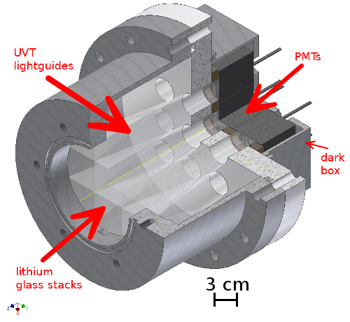
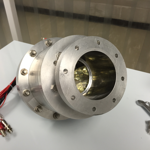
Figure 1: Three dimensional drawing of the UCN detector and enclosure (top), and a photo of the detector (bottom). The detector enclosure is made of Al, and the rim of the adapter flange which UCN can hit is coated with $1$ $\mu$m Ni by thermal evaporation (colour online).

2.2 ⁶Li Detector Signal Treatment

Signals from the PMTs are amplified by a Phillips 775 octal $10\times$ preamplifier and read out directly by 8-channel CAEN V1720 digitizers.

The CAEN V1720 has a PSD firmware that triggers on pulses below a certain threshold independently for each channel. The digitizer samples the waveforms every 4 ns, and for each sample digitizes the voltage on a $2$ V scale into an ADC value between 0 and 4096. Each channel of the digitizer triggers when a pulse goes some number of ADC counts below a pedestal value. The digitizer threshold for triggering was set at 250 ADC ($\sim-125$ mV).

The digitizer can be run with a fixed pedestal, or a pedestal taken from an average over the last 32 samples (128 ns). This self calculated pedestal is called a baseline in the digitizer documentation, and once a trigger happens, the baseline is held constant until the end of a specified gate time. The self-calculated baseline was used for the detector tests described in this paper.

For each trigger, the PSD firmware calculates the sum of the signal below the baseline starting from the trigger time for a short gate width, $t_{s}=40$ ns, and for a long gate width, $t_{L}=200$ ns. The short gate time has been chosen to contain all of the charge for gamma ray interactions in the light-guides. The ADC sum below the baseline within the short gate is called, $Q_{S}$, and the sum within the long gate is called, $Q_{L}$. The charge $Q_{L}$ contains the total charge deposit for neutron capture events. The PSD value is also calculated, and defined as:

$${\tt PSD}=\frac{(Q_{L}-Q_{S})}{Q_{L}}.$$ (2)

After each trigger, the digitizer channel is busy for a 150 ns dead-time. A cut on $Q_{L}$ and PSD provides a rejection of gamma interactions in the light-guides as described in Section 4.1. The PSD variable has been chosen to cancel out channel to channel variations in gain by making a ratio of charges. Also the PSD is sensitive to the difference in shape of the scintillation signals, and the signals from interactions in the light-guides.

The digitizer firmware stores only the $Q_{S}$, $Q_{L}$, PSD, baseline, and trigger time for each pulse, thereby permitting the V1720 to handle data rates up to $\sim$2 MHz without saturating the data path. The first seven tiles of the detector are read out on one digitizer, and the last two tiles are read out on a second digitizer. Each of the digitizers was connected by an independent optical fibre to a CAEN A3818 PCI Express card on the Data Acquisition (DAQ) computer for readout, allowing data rates up to 85 MB/s.

The time-stamp provided by the digitizer is a clock cycle count in 4 ns ticks up to 17 seconds. To help keep track of the time-stamp wrap-around, and check the digitizer synchronization, a $1$ Hz pulser was fed into the last channel of each of the two digitizers. In addition a signal from the PSI proton beam timing was sent into one of the channels of the detector to be used to determine the times when the proton beam arrived.

The DAQ software used the MIDAS system that is commonly used at PSI and TRIUMF. A MIDAS frontend for the CAEN V1720 was written to collect the PSD data from the digitizers and save it into MIDAS banks.

3 Detector tests with UCN

We used the two beamlines called “West-1” and “West-2” at the PSI UCN source [27]. West-2 offers the distinct feature that UCN have a dropping height of minimum 120 cm before reaching the detector. West-1 in a horizontal configuration provides UCN with energies starting above 54 neV given by the safety AlMg₃ foil in the beamline.

3.1 Time distribution

During August 2015 there was a 300 s UCN cycle at PSI, where the rate of UCN is highest right after a 3 second proton beam bunch on a neutron spallation target. For the next 297 seconds after the proton beam is turned off the UCN rate falls, going from rates of tens of kHz down to 20 Hz as seen in Fig. 2.

UCN rates on the West-1 beamline are a factor of 10 higher than on West-2. The operation mode was given by the priority of the nEDM experiment measuring at the third beam-port. Typically, UCN were only delivered to the West-1 beamport after 30 seconds, when the nEDM experiment stopped its filling period. During the UCN cycles the UCN propagate down the beam line to the experiment area. Typical UCN detector rates during 300 second UCN cycles in West-1 and West-2 measured in Aug. 2015 with our scintillation detector are shown in Fig. 2.

Note that our detector’s 75 mm diameter aperture does not match the 180 mm aperture of the West-1 beam-line, and that it can only see UCN above the Fermi potential of the scintillating glass (103.4 neV). This means that we see relatively more UCN from the vertical source, which has a spectrum starting at about 120 neV, matching our detector Fermi potential, than from the softer source of the horizontal West-1 beam. The PSI group has made measurements showing that on West-1, about 32% of the UCN are between 54 neV and 120 neV. Also, the two UCN cycles shown in the figure were taken on different days, and we know from measurements that during that time, the UCN source saw about a 15% decrease in the delivered UCN intensity. Therefore, we expect to see less than the 10$\times$ difference in UCN rate when comparing the distributions in Fig. 2.

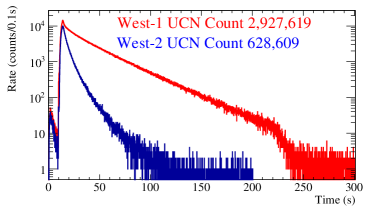
Figure 2: UCN observed during one UCN cycle, as detected with the ⁶Li UCN detector on West-1 (red) and West-2 (blue). The small peak before the main peak is caused by a 7 ms long pilot proton beam bunch used for checking the beam centering before the main beam bunch on the spallation target (colour online).

3.2 Charge measurement

The PSD versus $Q_{L}$ distribution from a UCN data run on West-1 beamline is shown in Fig. 3. The UCN signal events are centered around a PSD of 0.5 and $Q_{L}\sim 5000$ to $\sim 12000$, and signals from $\gamma$-rays in the lightguides are around $PSD\sim 0$. The values between these are due to pile-up effects, events right after the dead-time and late-light events. Further details on these effects are discussed in Section 4. Note that the negative PSD values come from pile-up and dead-time events. In these events, the average baseline calculated by the digitizer firmware is too large, resulting in the integrated $Q_{L}$ that it calculated becoming smaller than the $Q_{S}$. This feature of the PSD is also seen in simulations as described in Section 4.1.

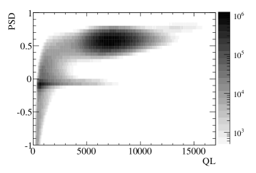
Figure 3: Event counts per bin are shown by the greyscale as a function of PSD and $Q_{L}$ from UCN data taken on the West-1 beamline.

The $Q_{L}$ distribution from each of the nine channels of the detector, with a PSD cut at 0.3 to eliminate the light-guide backgrounds, is shown in Fig. 4. These data are from twelve UCN cycles collected from the horizontal West-1 beamline. It is clear from these distributions that there is very little background remaining. The different numbers of counts seen is explained by the geometry of the detector. The corner square tiles are shadowed the most by the round aperture of the detector opening, giving them the lowest count.

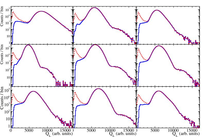
Figure 4: Event count per $Q_{L}$ bin from each of the nine channels of the ⁶Li scintillation detector from twelve cycles of UCN beam on the horizontal West-1 beamline. The distribution without a cut on PSD is shown as a dashed-red line, and with a cut on PSD$>0.3$ as the solid-blue line (colour online).

3.3 Channel to channel comparisons

In order to determine the rate stability of the detector, the ratio of the rates $R_{r}$ in the outer channels to the central channel is calculated. This ratio of rates is compared to the ratio of area ($R_{a}$) of the outer channel as measured from the photograph in Fig. 11 to the area of the central channel.

During each UCN cycle on the West-1 beamline that was used for this comparison, the ⁶Li detector counted $\sim 3\times 10^{6}$ neutrons corresponding to $\pm 0.06$% statisitical uncertainty. An overnight run containing 114 UCN cycles (9.5 hours) was taken to assess the rate stability. The count for each UCN cycle in each channel, and the ratio of counts per UCN cycle in each channel over the central channel was plotted versus UCN cycle to assess the rate stability. Fitting the ratio of count rates in each of the outer channels to a constant yielded an acceptable $\chi^{2}$ per degree of freedom as summarized in Table 2. The difference between the relative area and relative rate ($R_{a}-R_{r}$) is also tabulated.

We make two conclusions from these measurements. First is that the difference in efficiency between the channels is at most 5%. These differences could be due to differences in surface contamination or differences in the number and energy of UCN reaching the different tiles. In addition the good $\chi^{2}$/DOF demonstrates that the rate observed in each of the channels is stable. The statitstical uncertainty in the fit to a flat ratio of rates demonstrates an overall rate stability of 0.01% over the whole measurement period, and the statistical uncertainty on each cycle’s ratio of rates implies an uncertainty per cycle of 0.06%. The overall rate stability easily meets our goal of 0.03%, however the statistical uncertainty per cycle is not sufficient to evaluate whether short time scale variations are present at this level.

Table 2: Area relative to the central channel $R_{a}$, rate relative to the central channel $R_{r}$ as fit to 114 UCN cycles, $\chi^{2}$/DOF from the fit to a constant relative rate, and difference between the relative area and relative rate.

Channel	Rel. area ($R_{a}$)	Rel. rate ($R_{r}$)	$\chi^{2}$/DOF	$(R_{a}-R_{r})$
0	0.7490 $\pm$ 0.0018	0.7065 $\pm$ 0.0001	104.2/113	0.0425 $\pm$ 0.0018
1	0.2876 $\pm$ 0.0007	0.2849 $\pm$ 0.0001	119.7/113	0.0027 $\pm$ 0.0007
2	0.7634 $\pm$ 0.0018	0.7115 $\pm$ 0.0001	120.9/113	0.0519 $\pm$ 0.0018
3	0.3033 $\pm$ 0.0006	0.2809 $\pm$ 0.0001	119.4/113	0.0224 $\pm$ 0.0006
4	0.7495 $\pm$ 0.0017	0.7481 $\pm$ 0.0001	103.1/113	0.0014 $\pm$ 0.0017
5	0.2650 $\pm$ 0.0006	0.2771 $\pm$ 0.0001	132.9/113	-0.0121 $\pm$ 0.0006
6	0.7307 $\pm$ 0.0018	0.7075 $\pm$ 0.0001	100.3/113	0.0232 $\pm$ 0.0018
7	0.2672 $\pm$ 0.0007	0.2579 $\pm$ 0.0001	90.39/113	0.0093 $\pm$ 0.0007

4 Scintillation and light-guide background simulation

4.1 Digitizer simulation

In order to build probability distribution functions for scintillation due to neutron capture, $\gamma$-ray interactions in the the lightguides, late-light events, multiple signal events, and combinations of signal and background events, a detailed simulation of the voltage pulses from the lithium glass and of the digitizer PSD was developed. A single photo-electron (p.e.) in the PMT was assumed to produce a Gaussian pulse with a width, $\sigma_{pe}=6.4$ ns, an amplitude drawn from a Gaussian with mean and width, $A=20$ mV, with a minimum amplitude for a single p.e. of 4 mV. The pulse width $\sigma_{pe}$ was chosen to match the rise time of the scintillation signal in the lithium glass.

A single scintillation signal event’s pulse was then built assuming that the arrival times of each photo-electron from the scintillation signal followed a rise time, $\tau_{R}=6.4$ ns, a fast scintillation fall time, $\tau_{F}=41.7$ ns, and a slow scintillation fall time, $\tau_{S}=2000$ ns. The probability, $P(t)$, of having a photo-electron at a given time, $t$, when the scintillation light starts arriving at time, $T$, was drawn from the Probability Distribution Function (PDF):

$$P(t)=\left\{\begin{array}[]{l}A(1-{\tt e}^{-(t-T)/\tau_{R}}),\ \ T<t<T+5\tau_{R}\\ A((1-f_{L}){\tt e}^{-(t-T-5\tau_{R})/\tau_{F}}+\\ \ \ f_{L}{\tt e}^{-(t-T-5\tau_{R})/\tau_{S}}),\ \ t>=T+5\tau_{R}.\end{array}\right.$$ (3)

The number of photo-electrons for a single neutron event was drawn from a Poisson distribution with a mean number of photo-electrons of 83. The fraction of the scintillation light in the late-light was $f_{L}=1$%[28].

All of the values used in the simulation, as described above, were chosen to best match the PSD and $Q_{L}$ distributions in the data. This tuning was done by plotting the mean, sigma and mean over sigma of the $Q_{L}$ and PSD distributions in single dimension scans of the simulation parameters until the distributions matched these same values from the data distributions. The distribution of scintillation photo-electron arrival times along with a sample pulse is shown in the top panel of Fig. 5. Note that positive pulses with a threshold above a baseline were used in our simulation, while in the data the pulses are negative, and the threshold is some number of ADC below the baseline.

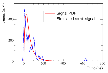
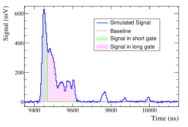
Figure 5: Simulated scintillation signal (blue dashed) and distribution function used to generate it (red solid) is shown in the top panel. The bottom panel shows the digitizer treatment of another simulated signal (solid line), where the baseline calculation (red dot-dashed line), signal within the short gate (green right-diagonal fill) and signal within the long gate (magenta left-diagonal fill) are shown (colour online).

The number of photo-electrons for the background signal was drawn from an exponential distribution with an average of $7.5$ photo-electrons. This distribution was chosen to match the dominant component of the background observed in data.

The matching of the single gamma background from the simulation and from data during times without UCN is shown in Fig. 6. The data distribution is used to represent the single gamma ray background from interactions in the scintillator and light-guide, as well as backgrounds from thermal neutrons. The distribution in the data has more counts at high $Q_{L}$ due to the presence of scintillation events in the lithium glass due to gamma-ray and thermal neutron interactions. The gamma ray background simulation is used for the simulation of pile-up of the gamma signals with themselves, and with the neutron signals.

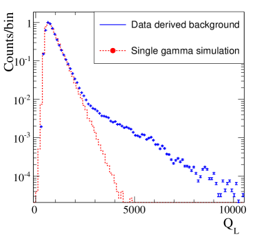
Figure 6: Background counts as a function of $Q_{L}$ from data taken during periods without UCN are shown as blue crosses, and is overlaid with the single gamma ray background shown as a red-dashed line (colour online).

These simulated data were then sent to a digitizer simulation described in the following section. The simulation of the pulses was used to generate 0.1 second long sets of data where the signal and background pulses were generated at a specified random rate.

4.2 Probability distribution functions from the simulations

Seven categories of events are considered. Self explanatory categories are single neutrons (1n), single backgrounds (1$\gamma$), pile-up of multiple signal neutrons (Nn), pile-up of multiple backgrounds (N$\gamma$), and pile-up of a single neutron with a background (1n1$\gamma$). After the end of a triggered event the digitizer channel is busy for 150 ns beyond the end of the long gate. If a neutron comes during this dead-time, part of its charge is not collected. We call these events single neutrons during the deadtime (1n deadtime). The last event type constitutes triggers on late-light from the scintillator (0n0$\gamma$).

Simulated electronic pulses for each of these possible combinations are shown in Fig. 7 and Fig. 8.

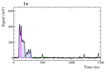
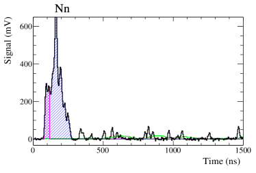
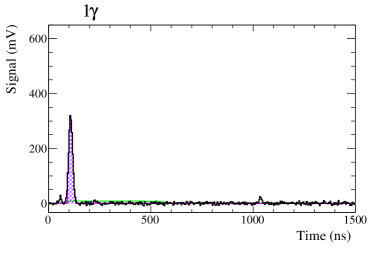
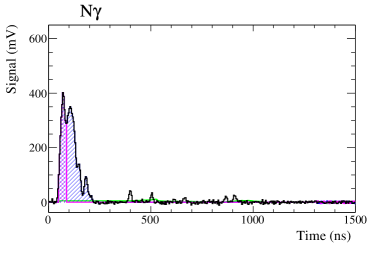
Figure 7: Simulated signals for different combinations of signal and background events. The magenta left-diagonal-hatched region represents the $Q_{S}$ portion of the signal, the blue right-diagonal-hatched region represents $Q_{L}$, and the green line (colour online) represents the average baseline. From top to bottom the plots show: 1n, Nn (2 neutrons), 1$\gamma$, and N$\gamma$ (3 $\gamma$) (colour online).

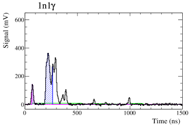
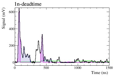
Figure 8: From top to bottom these plots show: a single signal plus single background event, a dead-time event, and a late-light re-trigger event (colour online).

The combination of the signal and background pulse simulations with the digitizer simulation is used to generate PDFs in the PSD versus $Q_{L}$ space for single neutron events, gamma events and different possible combinations pile up of events.

In the simulation, a a fixed (random) rate of 10 kHz of $\gamma$ interactions in the light-guides and 10 kHz of neutron interactions in the scintillator has been chosen. We separate out triggers that are from single interactions and put them in singles PDFs (1n, or 1$\gamma$ ). Triggers that have multiple interactions in the long-gate are put in multiples PDFs (Nn, N$\gamma$, and 1n1$\gamma$). By allowing the normalizations of these PDFs to be changed we approximately account for the varying rate during the UCN cycle.

In the case of the single background event, it was possible to use the data from cycles when no UCN are produced, as shown in Fig. 6. In our model we are assuming that background components from thermal neutrons and gamma-rays interacting in the scintillators are present in this PDF derived from data. The rest of the PDFs are derived from the simulations described above.

The PDFs for the different combinations of signal and background as found by the simulation are shown in Fig. 9 and 10.

The single neutron (1n) pulses extend out to the long gate integration time, meaning that their $Q_{L}$ will be larger than $Q_{S}$. The PSD is therefore greater than zero, and in this case is observed to be $\sim$0.5. A pile-up of two or more neutrons (Nn) has pulses at least as large as a single neutron, and can extend out to later time depending on the time separation between the two neutrons within the long integration time. The Nn events therefore have larger $Q_{L}$ than the 1n events, while $Q_{S}$ is unchanged. The Nn events therefore, on average, have a slightly higher PSD than the 1n events.

The single gamma (1$\gamma$) pulses fit within the short integration time, therefore they have similar $Q_{S}$ and $Q_{L}$ values. The PSD for these events is near zero. In fact, due to the settings of the digitizer, the PSD is slightly below zero due to the baseline shifting slightly down before the trigger time. This negative PSD effect becomes even more pronounced when looking at N$\gamma$, 1n deadtime, and 0n0$\gamma$ events where the baseline is shifted low due to the previous pulse on the channel. The 1n1$\gamma$ sample looks fairly similar to the 1n distribution, but there is some tail to higher $Q_{L}$ due to the additional light from the $\gamma$.

The 1n deadtime events do not integrate the full charge from the neutron pulse due to the trigger coming too late. For that reason the $Q_{L}$ for these events is lower than for the 1n events. These triggers come soon after the previous trigger, so the baseline is sometimes shifted low due to possible late-light of the previous pulse. The baseline shift can cause $Q_{L}$ to be lower than $Q_{S}$ causing some of these events to have negative PSD values.

Finally, the late-light pulses have low $Q_{L}$ and low $Q_{S}$, since they are triggers just above threshold. The small charges, and possible baseline shift leads to these events having a wide range of PSD values.

The data contain all of these different event categories, and some combination of these PDFs fills in the PSD versus $Q_{L}$ distribution observed in data. A template fit of these PDFs to estimate amount of signal and background in the data is possible.

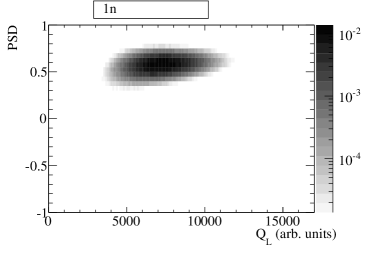
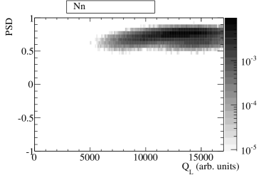
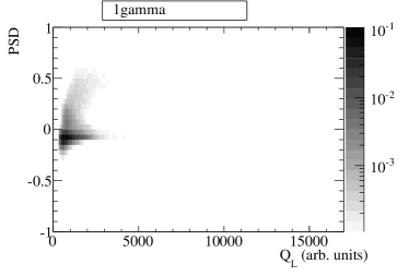
Figure 9: Event count (or relative event count) as a function of PSD and $Q_{L}$. From top to bottom: single neutron simulation, multiple neutron simulation, and background (from data from cycles without proton beam).

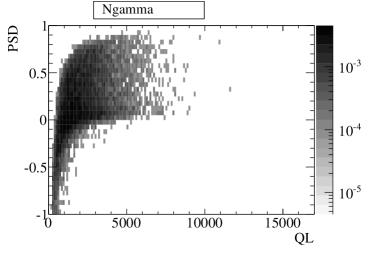
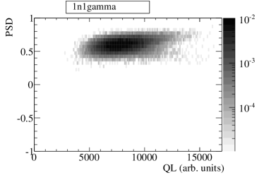
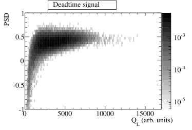
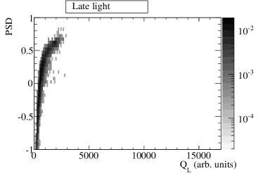
Figure 10: Event count (or relative event count) as a function of PSD and $Q_{L}$. From top to bottom: multiple background simulation, single neutron plus single background simulation, dead-time neutron simulation, and re-trigger on late-light simulation.

5 Estimate of the absolute detector efficiency and background contamination

To determine the ⁶Li detector’s UCN detection efficiency we consider the active area of the detector, losses due to absorption in the front face including the ⁷Li(n,$\gamma$)⁸Li reaction, and the transmission of the ⁶Li depleted layer. Neutrons lost due to the background rejection cuts are also considered. The effects of surface impurities is not straight forward to estimate and may affect the efficiency. The effects of surface impurities is estimated to be bounded by the 5% differences in relative rates of the channels presented in Section 3.3. The spectrum of UCN that are being detected also needs to be taken into account. Here we will assume that we want to know the efficiency for detecting UCN with kinetic energy far enough above the effective Fermi potential of the GS20 lithium glass ($\sim$ $103.4$ neV) so that we can neglect UCN reflection. The efficiency for detecting UCN with a known energy spectrum could then be estimated using a model for UCN reflection from a Fermi potential of 103.4 neV. Note that the Fermi potential of the GS30 (83 neV) is lower, and so should have negligible effect.

5.1 Detector effective area

The estimate of the detector’s effective area comes from a photograph of the detector’s front face, where the side length of each ⁶Li glass tile is $29.0\pm 0.1$ mm. Using this length the number of pixels in the photograph that make up the circular aperture of the detector are counted as the denominator, and the count of pixels containing ⁶ Li glass tiles as the numerator. From the photograph of the detector face shown in Fig. 11 in gray scale, the active area of the detector is estimated to be $97.4\pm 0.1$%.

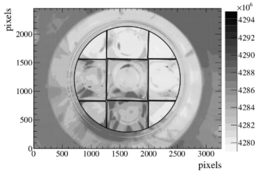
Figure 11: Picture of the detector face used for estimating the areal efficiency of the detector. The detector aperture and edges of the lithium glass are identified by the black lines.

5.2 Estimation of UCN absorption in Li depleted layer

Measurements of the transmission of UCN through different thicknesses of GS30 have been conducted by the LPC Caen group at the Institute Laue-Langevin in Grenoble [20]. Using their measurements for a $55\pm 10$ $\mu$m GS30 layer the UCN transmission is $92.6^{+1.2}_{-1.8}$%. The uncertainty is asymmetric due to the exponential nature of the attenuation through a layer with uncertain thickness. These results depend on the surface roughness and impurity present in the detectors of the LPC Caen group. Our detector’s lithium glass and surfaces were prepared by the same companies used by the LPC Caen group and therefore forms a good estimate for UCN losses in trasmission trough the depleted layer.

Part of the losses in the depleted layer occur due to the 6.6% of ⁷Li in the layer which allows neutron capture via ⁷Li(n,$\gamma$)⁸Li. Assuming a $1/v$ law for neutron cross sections from cold down to 100 neV UCN energy we estimate the UCN capture cross section on ⁷Li to be $\sigma\sim 6.0$ barns [29]. The effect is therefore fairly negligible since the fraction of UCN making it through $55$ $\mu$m GS30 due to (n,$\gamma$) reactions is 99.94%.

We conclude that the total UCN transmission of $92.6^{+1.2}_{-1.8}$% based on experimental results of the LPC Caen group accounts for all effects leading to losses of UCN in the GS30 layer.

5.3 PSD cut efficiency and background rejection

Estimates of the signal efficiency and background rejection due to the PSD versus $Q_{L}$ cut are estimated using an extended maximum likelihood fit of the PDF templates described in Section 4. The PDFs, binned in PSD and $Q_{L}$, are labelled as $P_{i}(PSD,Q_{L})$, where $i$=( 1n, Nn, 1$\gamma$, N$\gamma$, 1n1$\gamma$, 1n deadtime, or 0n0$\gamma$). The number of each type of event is estimated as $N_{i}$ by minimizing a negative log likelihood that is calculated as a sum over all $M$ of the PSD^j and $Q_{L}^{j}$ measurements in the data as:

$$-\ln{(L)}=\sum_{i}^{7}N_{i}-\sum_{j}^{M}\ln{\sum_{i}^{7}P_{i}(PSD^{j},Q_{L}^{j})}.$$ (4)

The data used were taken on West-1 for the time period from the start of the three second proton beam. Data were taken from all channels for times 10 s to 280 s as shown in Fig. 2. The first three seconds of this data include a gamma flash and fast neutrons. Note that the single gamma background should include these backgrounds as well, since they are taken over the sime time period where the proton pulse has come, but the UCN gate valve was closed.

A projection of the fit results onto the PSD and $Q_{L}$ axes is shown in Fig. 12. All of the features seen in the data are reproduced in the fit, although the chi-squared per degree of freedom (DOF) of the fit is rather poor ($\chi^{2}$/DOF $=775596/140$ in $Q_{L}$ and $\chi^{2}$/DOF $=6.68\times 10^{8}/20$ in PSD). We attribute the differences between the simulation and data to details that are not properly modelled, such as any contribution from light leaks, and PMT after-pulsing. For the $Q_{L}$ distribution, differences in gain between the nine channels of the detector may contribute.

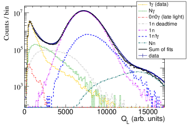
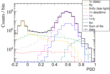
Figure 12: Template fit results in the one dimensional projections along the total event charge (top) and along the PSD (bottom) (colour online). These data are from the start of the main proton beam pulse, from 10 s to 280 s in the UCN cycle.

5.4 Cut detection efficiency and background rejection estimates

Using the template fit, the neutron detection efficiency and background contamination are computed for different cut values in PSD and $Q_{L}$. The PDFs representing neutron signals include single neutron (1n), multiple neutrons (Nn), dead-time neutrons (1n deadtime), and single neutron single gamma (1n1$\gamma$). The background rates are extracted from the single gamma (1$\gamma$), late-light (0n0$\gamma$), and multiple gamma (N$\gamma$) templates. If the total number of neutrons in the templates is $N_{n}$, and the number of neutrons above a given cut value is $N_{n}^{cut}$, then the neutron efficiency due to background rejection cuts is defined as:

$$\epsilon_{n}=\frac{N_{n}^{cut}}{N_{n}}.$$ (5)

If the number of events in the background templates above a given cut value is $N_{\gamma}^{cut}$, then the background contamination fraction is defined as:

$$\eta_{\gamma}=\frac{N_{\gamma}^{cut}}{N_{n}},$$ (6)

and the background rejection as:

$$\epsilon_{\gamma}=1-\eta_{\gamma}.$$ (7)

Figure 13 shows the neutron efficiency and background contamination during the entire UCN cycle for two PSD cut values. For higher cut values, the efficiency is slightly reduced, but the background contamination is also reduced.

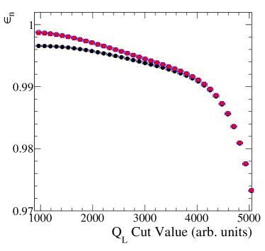
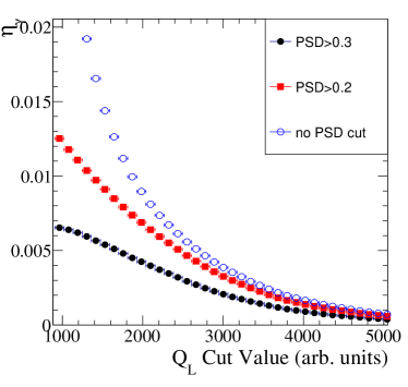
Figure 13: Neutron cut efficiency (top panel) and background contamination (bottom panel) for different cuts on $Q_{L}$. In both panels the blue open circles have no PSD cut, the red squares are with cut on PSD$>0.2$, and the black circles are for a cut on PSD$>0.3$ (colour online).

The neutron and background rates vary over UCN cycle. To study the neutron detection efficiency and background contamination at different rates on the West-1 beamline, the data was split into three time periods during the UCN cycle: high rates of 100 kHz to 50 kHz at times between 0 s an 10 s after the proton beam arrives, middle rates of 50 kHz to 20 kHz at times between 10 s and 40 s, and low rates of 20 kHz to 100 Hz beetween 40 and 270 s. Each of these data sets was fit using the template fit and then the efficiency was calculated with cut on PSD$>0.3$ using the parameters from each fit. As shown in Fig. 14, the high rate data had more background contamination than the other rates, due to the larger fraction of events with pile-up effects, and due to the proton beam being on for the first three seconds. The lowest rate data has a higher contamination than the mid-rate events due to the higher ratio of background to signal events. Using a cut on $Q_{L}>3000$ ADC and PSD$>0.3$, the neutron efficiency was $99.5\pm 0.5$% and the background contamination was $0.3\pm 0.1$%.

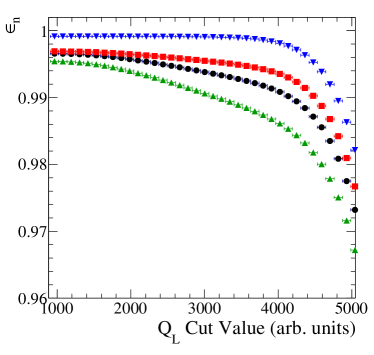
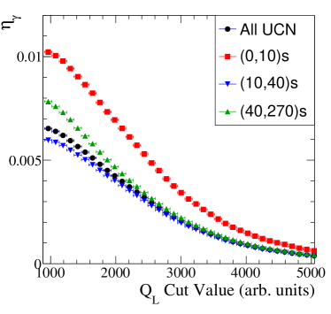
Figure 14: Neutron cut efficiency (top panel) and background contamination (bottom panel) for different times since the UCN production. Shown in black are all UCN from 0 s to 270 s after the proton beam turns off. The red boxes are for high rate over the first 10 s after the proton beam starts, the blue downward-triangles are for middle rate UCN over the next 30 s, and the green upward-triangles are for low rates over the last 230 s. These plots have a cut PSD$>0.3$ (colour online).

The ⁶Li detector therefore has a very good background rejection due to the signal shape variation between light-guide background (Cerenkov events) and the scintillation events from the lithium glass.

5.5 Overall Detector Efficiency Estimate

The overall detection efficiency, for the UCN rates and energies available at the West-2 beamport, including effects of GS30 transmission, effective area, and background rejection, is $89.7^{+1.3}_{-1.9}$%, which is dominated by the uncertainty in the absorption in the GS30 layer. The transmission measurement of the GS30 was performed by the CAEN group at ILL, with a different UCN energy spectrum, and so there remains the caveat that this efficiency is for UCN energies above the Fermi potential of the ⁶Li glass. The effects of surface imperfections is not included in this estimate, and is a possibly the source of the differences between the relative rates observed between the different channels of the detectors when compared to the area they present to the UCN beamline.

The rate dependent portion of the uncertainty, which is most concerning to measurements requiring a stable rate, could be improved by applying the statistics of random signals and backgrounds to model the expected rates. This would represent an improvement to the simple fit with unconstrained fractions of different types of pile-up described in this paper.

6 Relative rate comparison

6.1 Comparison to Cascade detector

A y-shaped UCN beam splitter to divide the UCN evenly into two ports was used on the West-2 beamline at PSI to compare the rates of UCN detected by a Cascade detector and our ⁶Li detector. The detectors in this y-configuration are shown in Fig. 15.

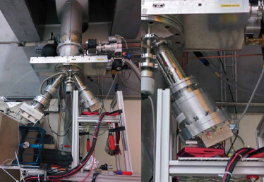
Figure 15: Configuration for splitting the UCN into two detectors on the West-2 beamline. The Cascade detector is on the left and the ⁶Li detector is on the right (colour online).

The connection of the ⁶Li detector to the y-shaped beam splitter was a 20 cm long NiMo coated guide with a diameter of 75 mm. The Cascade detector has a 110 mm diameter aperture, and two adapter flanges were needed to go from 110 mm to 70 mm to 75 mm to connect to the other side of the y-configuration. The Cascade detector therefore sits $\sim 20$ cm lower than the lithium glass detector and has a longer path for the UCN to pass.

6.2 Cascade Detector

The Cascade UCN detector is a GEM-based neutron detector with a single 200 nm thick layer of ¹⁰B deposited on a 100 $\mu$m thick aluminum entrance foil. The boron captures neutrons and releases an $\alpha$ and ⁷Li particle,

$${}^{10}B+n\rightarrow\alpha+{{}^{7}}Li.$$ (8)

An Ar/CO₂ mixture is used as a detection gas. Due to the low Z materials, this detector picks up negligible $\gamma$ background. The employed detector has a $10\times 10$ cm² square shaped sensitive area which is divided into 64 individually read out pixels. The detector comes with its own proprietary data acquisition system. The data acquisition is based on a complex pattern recognition algorithm which is performed online in the detector’s FPGA electronics. This allows the software to define what patterns are accepted as a neutron event.

6.3 Overview of the Measurement Method

Both detectors were placed in the y-configuration at the West-2 port to allow for a comparison of the averaged UCN rate over the course of the beam cycle for both detectors. The timing calibration between the two detectors’ Data AcQuisition (DAQ) was done at the few second level by comparing the time reported by the DAQ computers. A closer matching of the time in the analysis of the data was performed at about the 0.05 s level by aligning the times when the UCN rate was increasing when the main proton beam arrives, corresponding to times around 10 s in Fig. 2.

The top panel of Fig. 16 shows UCN counts detected by both detectors in each cycle. The ⁶Li detector counts are after cuts on $Q_{L}>3000$ and PSD¿0.3 were applied. We observe that during the course of the measurement, the UCN count from the PSI source was changing, and that both detectors track this change in the same way. The smallest aperature that the UCN must pass to get to the detectors is used as a worst case scaling of the counts seen by the 6-Li detector. The scaling is used to calculate a normalized count to compare with the Cascade detector. The ratio of the areas used in the scaling is $(70$ mm$/75$ mm$)^{2}=0.871$. The bottom panel of Fig. 16 shows a ratio of the area normalized count in the ⁶Li detector to the count in the Cascade detector. This comparison shows that for the spectrum of UCN in this beamline the ${6}$Li detector had at least $10.279\pm 0.024$(stat)% more counts than the Cascade detector.

The additional flanges required to adapt the Cascade detector to the $75$ mm diameter y-configuration introduce a large uncertainty in measuring the Cascade counting rate. A GEANT4 UCN simulation of the y-configuration was prepared, using NiMo Fermi potential of 235 neV for the beampipes and adapter flanges. The number of UCN reaching each detector was found to strongly depend on the assumed initial UCN spectrum reaching the entrance of the y-configuration ports. We therefore conclude that the ⁶Li detector is at least as efficient as the Cascade detector, but that the difference in UCN counts that we observed could entirely be due to the additional flanges required for the Cascade detector.

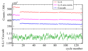
Figure 16: Detector count per UCN cycle is shown in the top panel for the ⁶Li detector by red filled circles after cuts on $Q_{L}>3000$ and PSD¿0.3, the Cascade detector by blue filled squares, and the area normalized ⁶Li count by magenta open circles. The bottom panel shows the ratio of the area normalized count in the ⁶Li detector to the Cascade detector (colour online).

The UCN detection rate in 0.1 second bins since the beginning of the 300 s UCN cycle averaged over 130 beam cycles is compared in Fig. 17. Again the ⁶Li detector counts are after cuts on $Q_{L}>3000$ and PSD¿0.3. This comparison includes the area normalization and shows that ⁶Li detector detect more UCN at higher rates near the beginning of the UCN production than the Cascade detector. During the course of the UCN cycle the energy spectrum of the UCN reaching the detectors changes: the faster UCN reach the detectors sooner, and later in the beam cycle, the slower UCN reach the detectors. The ⁶Li with effective Fermi potential of 103.4 neV does not detect the slowest UCN, making the Cascade detector more efficient for lower energy UCN (down to the 55 neV of Al).

We conclude that the ⁶Li detector has a detection efficiency at least as large as the Cascade detector for UCN with energies above the Fermi potential is 103.4 neV.

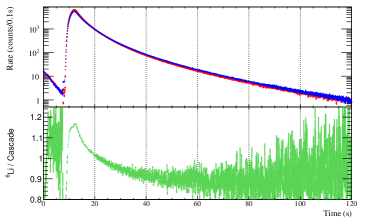
Figure 17: The top panel shows the counts per 0.1 s bin averaged over 130 UCN cycles for the area normalized ⁶Li detector (red) and the Cascade detector (blue). The bottom panel shows the ratio of counts in the ⁶Li detector to the Cascade detector (colour online).

7 Conclusion

In this paper we have presented a ⁶Li-based fast scintillation counter and a detailed electronics simulation which has been used to estimate the detector efficiency and background rejection for the data collected at the PSI UCN source. The absolute detector efficiency is found to be $89.7^{+1.3}_{-1.9}$%, with a background contamination of $0.3\pm 0.1$%. Using comparisons of UCN rates from the different tiles of the ⁶Li detector, we have demonstrated that the detector is stable at the 0.06% level or better, and that the variation in efficiency between the detector tiles is less than 5%. Finally we have shown that the ⁶Li detector is at least as efficient as the Cascade detector for UCN with energies above the Fermi potential of the lithium glass. Counting rate differences observed between the two detectors can be entirely explained by the additional flanges needed to connect the detectors to the same UCN beamline.

8 Acknowledgements

We acknowledge support of the National Science and Engineering Research Council (NSERC) and Canadian Foundation for Innovation (CFI) in Canada. We thank our colleagues at PSI for allowing us to conduct the detector tests at their facility. We thank staff and colleagues at TRIUMF who have provided support and feedback in the design and testing of the detector. We are grateful to Andrew Pankywycz at the University of Manitoba who machined the light-guides and aluminium detector housing. Finally we thank University of Winnipeg technician David Ostapchuck who helped with various aspects of the design and construction of the detector.

References

- [1] Pospelov, M., Ritz, A.: Electric dipole moments as probes of new physics. Annals of Physics 318 (2005)
- [2] Filippone, B.: New searches for the neutron electric dipole moment. Physics of fundamental Symmetris and Interactions at low energies, PSI2013 (2013)
- [3] Wohlmuther, M., et al.: The spallation target of the ultra-cold neutron source UCN at PSI. Nucl. Instr. and Meth. A 564 (2006)
- [4] Serebrov, A.P., et al.: New measurements of neutron electric dipole moment with double chamber EDM spectrometer. JETP Letters 99 (2014)
- [5] Serebrov, A.P., et al.: Supersource of ultracold neutrons at WWR-M reactor in PNPI and the research program on fundamental physics. Physics Procedia 17 (2011)
- [6] Kirch, K.: EDM searches. AIP Conference Proceedings 1560 (2013)
- [7] Baker, C.A., et al.: The search for the neutron electric dipole moment at the Paul Scherrer Institute. Physics Procedia 17 (2011)
- [8] Masuda, Y., et al.: Spallation UCN production for nEDM. Physics Letters A 376 (2012)
- [9] Altarev, I., et al.: Program for studying fundamental interactions at the PIK reactor facilities. Nuovo Cimento C 35 (2012)
- [10] Golub, R., Lamoreaux, S.K.: Neutron electric-dipole moment, ultracold neutrons and polarized 3He. Physics Reports 237 (1994)
- [11] Ito, T.M.: Plans for a neutron EDM experiment at SNS. J.Phys. Conf. Ser. 69 (2007)
- [12] Kawasaki, S.: 2nd generation He-II UCN source. Presented at CP violation in elementary particles and composite systems, RCNP, Osaka (2014)
- [13] Martin, J.W.: TRIUMF facility for a neutron electric dipole moment experiment. AIP Conference Proceedings 1560 (2013)
- [14] Lauss, B.: A new facility for fundamental particle physics: The high-intensity ultracold neutron source at the Paul Scherrer Institute. AIP Conference Proceedings 1441 (2012)
- [15] Lauss, B.: Commissioning of the new high-intensity ultracold neutron source at the Paul Scherrer Institute. Hyperfine Interactions 211 (2012)
- [16] Lauss, B.: Ultracold neutron production at the second spallation target of the Paul Scherrer Institute. Physics Procedia 51 (2014)
- [17] Ban, G., et al.: UCN detection with 6Li-doped glass scintillators. Nucl. Instr. and Meth. A 611(280) (2009)
- [18] Ban, G., et al.: First tests of 6Li doped glass scintillators for ultracold neutron detection. J. Res. Nat. Instr. Stand. Technol. 110 (2005)
- [19] Afach, S., et al.: A device for the simultaneous spin analysis of ultracold neutrons. European Physical Journal A 51 (2015)
- [20] Ban, G., et al.: Ultracold neutron detection with 6Li-doped glass scintillators. arXiv:1606.07432 (2016)
- [21] Spowart, A.R.: Neutron scintillating glasses: Part 1. Nucl. Instr. and Meth. A 135 (1976)
- [22] Jamieson, B., Rebenitsch, L.A.: Determining the 6Li doped side of a glass scintillator for ultra cold neutrons. Nucl. Instr. and Methods A 790 (2015)
- [23] Atkinson, M.: Initial tests of a high resolution scintillating fiber (scifi) tracker. Nucl. Instr. and Meth. A 254 (1987)
- [24] Brollo, S., Zanella, G., Zannoni, R.: Light yield in cerium scintillating glasses under x-ray excitation. Nucl. Instr. and Meth. A 293 (1990)
- [25] Sakamoto, S.: A Li-glass scintillation detector for thermal-neutron TOF measurements. Nucl. Instr. and Meth. A 299 (1990)
- [26] Goeltl, L., et al.: An endoscopic detector for ultracold neutrons. Eur. Phys. J. A 49 (2013)
- [27] Lauss, B.: UCN beamlines at PSI. PSI internal document, Paul Scherrer Institut (2014)
- [28] Murata, T., et al.: Fast-response and low-afterglow cerium-doped lithium 6 fluoro-oxide glass scintillator for laser fusion-originated down-scattered neutron detection. IEEE Trans. on Nucl. Science 59 (2012)
- [29] Heil, M., Käppeler, F.: The (n,) cross section of 7Li. The Astrophysical Journal 507 (1998)