Critical Behaviour of Spanning Forests
on Random Planar Graphs

Abstract

As a follow-up of previous work of the authors, we analyse the statistical mechanics model of random spanning forests on random planar graphs. Special emphasis is given to the analysis of the critical behaviour.

Exploiting an exact relation with a model of $\mathrm{O}(-2)$-loops and dimers, previously solved by Kostov and Staudacher, we identify critical and multicritical loci, and find them consistent with recent results of Bousquet-Mélou and Courtiel. This is also consistent with the KPZ relation, and the Berker–Kadanoff phase in the anti-ferromagnetic regime of the Potts Model on periodic lattices, predicted by Saleur. To our knowledge, this is the first known example of KPZ appearing explicitly to work within a Berker–Kadanoff phase.

We set up equations for the generating function, at the value $t=-1$ of the fugacity, which is of combinatorial interest, and we investigate the resulting numerical series, a favourite problem of Tony Guttmann’s.

Dedicated to Tony Guttmann, on the occasion of his 70th birthday.

1 Introduction

1.1 Spanning Forests and the Potts Model

A spanning forest $F$ over a graph $G$ is a spanning subgraph without cycles, thus each of its connected components is a tree. For a graph $G$, a set $\vec{w}=\{w_{e}\}$ of edge weights, and a parameter $t$, the partition function of spanning forests $Z^{\mbox{\scriptsize{forest}}}_{G}(t,\vec{w})$ on a graph $G$ is defined as

$$Z^{\mbox{\scriptsize{forest}}}_{G}(t,\vec{w}) =\sum_{F\preceq G}t^{K(F)}\prod_{(ij)\in E(F)}w_{ij}\,.$$ (1)

where the sum on $F\preceq G$ means on all spanning forests over $G$, and $K(F)$ is the number of trees in the forest.

Models in this class are both of combinatorial interest in Graph Theory, as first considered by the seminal work of Tutte and Whitney before the war [1], and of interest in Critical Phenomena, as they arise as particular limit $q\to 0$ of the $q$-colour Potts Model in the Fortuin–Kasteleyn representation [2]. The limit $t\to 0$ in (1) corresponds to spanning trees, an even more studied model, whose history dates back to the 19th century.

On a fixed (weighted) graph $G$, spanning forests can be mapped through a fermionic Berezin integral to an $\mathop{\mathfrak{osp}}\nolimits(1|2)$-invariant $\sigma$-model (or O$(n)$ $\sigma$-model analytically continued to $n=-1$) and its critical behaviour on a square lattice [3] and on the triangular lattice [4] has been deduced, in the range $t\geq 0$. In this range, RG calculations in dimension two show the absence of critical points between $t=0$ and $t\nearrow+\infty$, and a flow from $t=0$ towards $t=+\infty$ compatible with asymptotic freedom. The exact solution of the Potts Model on regular two-dimensional lattices (which are Yang–Baxter integrable) [5] also suggests the absence of critical points in this range. The picture is best understood in the case of the square lattice. In this case, the second-order ferromagnetic transition of the Potts Model, in the phase space parametrised by $(q,v)$, occurs on the parabola $\Gamma_{\rm F}$, defined as $v=+\sqrt{q}$ for $0\leq q\leq 4$. Parametrising $q=4\cos^{2}(\pi/\delta)$, the central charge of the associated conformal field theory is $c=1-\frac{6}{\delta(\delta-1)}$. No other critical lines are expected in the quadrant $q,v\geq 0$, this implying the forementioned behaviour for spanning forests at positive fugacity, and consistently the well-known behaviour of uniform spanning trees as a logarithmic non-unitary CFT with $c=-2$.

On the other side, the solution of the Potts model predicts the existence of a complex critical behaviour in the anti-ferromagnetic regime $-1\leq v<0$ (and the non-physical one $v<-1$), i.e. in the quadrant $q\geq 0$ and $v<0$, which corresponds, for spanning forests, to finite negative values of $t$. The solution predicts two other dual curves $\Gamma_{\rm AF}^{\pm}$, namely $v=-2\pm\sqrt{4-q}$, where the anti-ferromagnetic criticality occurs, and is identified with a CFT with $c=2-\frac{6}{\delta}$ with the peculiar presence of a non-compact boson (thus $c=-1$ for spanning forests, obtained for $\delta=2$). On top of this, it predicts yet another special curve, $\Gamma^{\prime}_{\rm F}$, defined as $v=-\sqrt{q}$, all of this still in the range $0\leq q\leq 4$. At $\Gamma^{\prime}_{\rm F}$ there is a different behaviour, and a CFT with $c=1-\frac{6(\delta-1)^{2}}{\delta}$, (i.e., peculiarly, yet again $c=-2$ for spanning forests). In a series of works, Saleur and Jacobsen [7, 8, 9] have tried to clarify the nature of this transition, and its CFT content. However, a number of subtleties arise (role of the twist parameter in the boundary conditions of the associated spin chain, saddle-point approximation and ansatz in the study of the Bethe equations, special behaviour at the Beraha numbers, …), so that the picture is surely quite complicated, and possibly in part still conjectural.

Something that seems well-established, and was predicted already in [6, 7], is the existence of a Berker–Kadanoff phase, i.e. a full interval of couplings with the critical exponents of the self-dual curve $\Gamma^{\prime}_{\rm F}$, for all points between $\Gamma_{\rm AF}^{+}$ and $\Gamma_{\rm AF}^{-}$. Planar duality exchanges $v=0$ with $v=\infty$, leaves fixed $\Gamma_{\rm F}$ and $\Gamma^{\prime}_{\rm F}$, and exchanges $\Gamma^{\pm}_{\rm AF}$ (thus leaving fixed the predicted Berker–Kadanoff interval). The picture in the triangular lattice, which is also Yang–Baxter solvable, seems to be analogous, but universality is not clear and is probably absent in some respect (see in particular the discussion in [10] and the recent work [11]), and it is probably fair to say that the Potts phase diagram, for general two-dimensional periodic lattices and out of the (simpler) ferromagnetic quadrant, deserves investigation still nowadays.

Figure 1 summarises the main elements described above, for the case of the square lattice. For a more detailed account of this complicated landscape, the reader may consult the introduction of [12] , and, for more details on the triangular lattice, of [10]. For the behaviour of spanning forests, introduction and conclusions of [8] are a valuable reference. Some more comments, and relations with the results of this paper, are discussed in Section 7.

Figure 1: The phase diagram of the Potts model on the square lattice. There are three regions, corresponding to a ferromagnetic phase (F), a high-temperature phase (HT), and an anti-ferromagnetic/non-physical Berker–Kadanoff phase (BK). On the right, we show the phase diagram for spanning forests, as a magnification of the neighbourhood of $(q,v)=0$. In this model we have a single parameter left, the ratio $t=q/v$ by which limit $q,v\to 0$ is taken in the Potts model. Thus, the parameter $t$ may be represented by half of a circle, i.e. $t=\tan\theta$, and $\theta\in[-\pi/2,\pi/2]$. Arrows on the circle denote the behaviour under the Renormalisation Group. The value of $t_{\ast}$ is $-4$.

1.2 Statistical mechanics on Random Planar Graphs

Versions of statistical mechanics models on random planar graphs are often solvable through methods of Random Matrices [13, 14, 15, 16], and, mainly in the 80s and 90s, a number of well-known statistical mechanics models have been solved in this framework (Ising, Potts, O$(n)$ Loop Models,…). These models correspond to the annealed average, of the fixed-graph partition function for a graph $G$, over the ensemble of all planar graphs $G$ with the grand-canonical measure $g^{|V(G)|}$. So, given a class $\mathcal{G}=\{G\}$ of planar graphs (e.g., all planar graphs with vertices of prescribed degree), and a fixed-graph partition function $Z_{G}(t)$ for a certain model, possibly depending on some global parameters $t$ (like the temperature, or, here, the component fugacity), the random planar graph related quantity is

$$Z^{\rm rpg}(t,g):=\sum_{G\in\mathcal{G}}\frac{1}{|\mathop{\mathrm{Aut}}\nolimits(G)|}g^{|V(G)|}Z_{G}(t)$$ (2)

(here $|\mathop{\mathrm{Aut}}\nolimits(G)|$, the cardinality of the group of planar automorphisms of the graph $G$, is introduced for convenience, and is irrelevant in the thermodynamic limit).

Besides being interesting per se, a solution to such a model is also relevant in understanding the phase diagram and critical exponents in regular two-dimensional geometries, in light of the Knizhnik, Polyakov, Zamolodchikov (KPZ) relation [17, 18, 19, 20].

In some, more rare, cases, a better analytic control on the solution can be achieved by an alternate approach, that, instead of using Random Matrices, makes use of combinatorial recursions [16]. These are inspired by the Tutte solution of the original counting problem in the 60’s (the quadratic method), but are not confined to this, as recent years have seen a flourishing of exact combinatorial approaches, as in [21, 22, 23] or in [24, 25, 26].

It is thus natural to ask whether the problem of spanning forests is also solvable on random planar graphs. The fact that this model is a limit of the Potts Model, and that some aspects of the latter on random planar graphs are known exactly (there is a large literature on the subject, starting with [27]), might seem to suggest that the solution of the Potts Model already provides a complete answer. However, this is not the case, because of the analytic structure of this solution (that is explicitly calculated only on a discrete set of values for $q$, or on the self-dual critical curve, analogue of $\Gamma_{\rm F}$), and of the peculiar difficulties pertinent to the way in which the spanning-forest limit is taken. Even when the approach is of combinatorial nature [28, 29, 30], the present understanding of the full Potts Model is too fragmentary for deducing the behaviour of spanning forests just by specialising the general results, and it is instead advisable to exploit from the beginning the simplifying properties of the forest case.

Yet another ansatz could have been based on the forementioned relation with the $\mathrm{OSP}(1|2)$ non-linear $\sigma$-model, and, by the Parisi–Sourlas mechanism, the equivalence of the latter, at the perturbative level, with the O$(n)$ model, analytically continued at $n=-1$. Also this is not the case, due to the fact that the O$(n)$ model related to spanning forests, and the one which is solved on random planar graphs, have an important difference: the former is a model with an extra $\mathbb{Z}_{2}$ symmetry, i.e. it is a projective $\sigma$-model, while the latter is the O$(n)$ ‘Nienhuis Loop Model’, which does not have this symmetry, see the discussion in [31].

To some surprise, instead, (see however the discussion of Section 3.1), the solution of the O$(n)$ Loop Model at $n=-2$ is relevant here. Indeed, a first approach has been presented by two of the authors in [32] . This approach is based on an exact combinatorial relation with a O$(n)$ Loop Model, which, in the case corresponding to random triangulations, had already been solved by Kostov and Gaudin [33, 34]. This led, in particular, to the first determination of the radius of convergence for spanning forests on random planar graphs, at fugacity $t=-1$, i.e. in the anti-ferromagnetic region, to be $g_{c}=\pi/(8\sqrt{6})$, remarkably a value whose algebraic nature is incompatible with the $D$-finiteness of the corresponding generating function (see the pertinent discussion in [35]).

Our approach was not completely satisfactory. The combinatorial part is exact, and performed for arbitrary $p$-angulations, but the solution is not self-contained, as it is based on the forementioned former solution of Kostov. The original specialisation to the cubic case can be extended, in part, by use of later results by Kostov and Staudacher [36] (a task done here), however an issue remains unsolvable: the solution by Kostov and Staudacher is done at the level of the saddle-point approximation of the Random-Matrix integral, which is the solution method with the smallest amount of mathematical control, e.g. on finite-size corrections (w.r.t., e.g., the use of orthogonal polynomials, and, no telling, w.r.t. explicit bijective approaches).

A quite satisfactory full solution has been presented by Bousquet-Mélou and Courtiel in [35] (see also [37]). It turns out that the simplest case corresponds to $p$-angulation with $p$ even (and, among these, quadrangulations are the best example). Nonetheless, the authors manage to solve also the case of triangulations. Their approach relies strongly on a general recursive decomposition invented by Bouttier and Guittier [26]. Said in a few words, there exist explicit bivariate hypergeometric series, $\theta$ and $\phi_{1,2}$, such that (the derivative of) the generating function $F(z,u)$, satisfies a system of three equations, of the form

$$F^{\prime}(g,t) =\theta(R,S)\,, R =g+t\,\phi_{1}(R,S)\,, S =t\,\phi_{2}(R,S)\,.$$ (3)

A remarkable and surprising result of [35] is that, in a full range of fugacities, including $-1\leq t<0$ and possibly extending below $t=-1$, the generating function has a string susceptibility distinct from the one of pure gravity, and shows peculiar inverse-logarithmic corrections.

Note that such a behaviour appears to be new within models of random planar graphs, which are exactly-solved through methods of bijective combinatorics and recursive decompositions. This is at no surprise, as such an ‘exotic’ behaviour would be impossible in a ‘simple’ random-matrix model, with a single matrix and a polynomial potential. In this case, it emerges in connection to the structure of the system of equations of Bouttier and Guittier, in vicinity of a singularity in the complex plane.

This is thus in contradiction with the simplest picture of models of Quantum Gravity with matter, which, by KPZ, are supposed to be analogous to their Euclidean counterparts, that, in turns, under the assumption of generality of the critical manifold in the phase space, shall show criticality on a manifold of co-dimension one in the phase space.

However, as we have already discussed above, the modern comprehension of the phase diagram of the Potts model does not follow this simple pattern. In particular, in the anti-ferromagnetic region we have a Berker–Kadanoff phase, with the same exponents as the theory at its edges, with the exception of one special point (and, in our case, the same exponents of spanning trees). Thus, the fact that the string susceptibility takes a constant non-trivial value in a whole interval all along $t\geq 0$ is in perfect agreement with Saleur’s prediction of the Berker–Kadanoff phase, and the KPZ correspondence. On the contrary, the presence of inverse powers of logarithms, to our knowledge, couldn’t be predicted in advance by general arguments (and may be present only as a speciality of the $q=0$ case, where the critical behaviour is a logarithmic CFT, but we cannot conclude on this point).

To our knowledge, in retrospect, the result of [35] is the first case in which the KPZ counterpart of a Berker–Kadanoff phase has been observed to be valid in a mathematically rigorous way, thus producing a highly non-trivial check of the KPZ correspondence, which still nowadays is considered quite mysterious.

1.3 Plan of the paper

This paper is a natural continuation of the investigation of the model started in [32]. On one side, it uses essentially the same main tool, namely the correspondence with the O$(n)$ loop model and the saddle-point solution of the latter by Kostov and Staudacher [36], either directly, or as a guideline for performing a more extensive analysis. On the other side, this calculation is now performed while having in mind the procedure in [35]. We will see that interesting connections between the two derivations will emerge in the treatment.

As we said, the approach of [35] is completely rigorous. Which is good, of course, but, as a side effect, the authors refrain from extending their analysis to situations in which it shall be supplemented by widely believed (but not rigorously proven) further hypotheses. An example is the fact that, in the cubic case, the authors claim the appropriate behaviour only for Cesàro means of the coefficients, see [35, Remark 1, page 46]. Another example is that the authors do not try to extend the analysis to $t<-1$, where a certain positivity property (discussed later on in Section 6) is lost.

We make here a different choice. We believe that the phase diagram of the model under consideration is still puzzling, with questions which are genuinely open. So we find it useful to establish reasonable derivations, even, if necessary, at the expenses of mathematical control. We rederive all the main results of [35], extend the analysis to all the range of $t$, and determine the presence of a critical value $t_{\ast}<-1$, which we identify with the other endpoint of the Berker–Kadanoff phase. Along the derivation, we determine an analytic expression for the spectral density, a result partially contained in [36], but clearly not in [35] (where there is no interpretation of the results in terms of random matrices).

Our methods are intrinsically less rigorous than the ones in [35]. Nonetheless, given the increase of combinatorial methods for dealing with O$(n)$ models in full rigour, also from the point of view of random matrices, [38, 39, 40], it is conceivable that, in future, our approach can also be improved to the appropriate level of mathematical rigour.

In Section 2 we will review the derivation of a matrix integral for the spanning-forest model. In Section 3, we establish the mapping of the model onto the O$(n=-2)$ gravitational loop model. This corrects a mistyped formula in [32]. In Section 4, which is the main part of the paper, we complete the analysis of the model, started in [32]. In passing, we see the emergence of connections with the quantities which are relevant in the (apparently orthogonal) approach of [35]. Sections 5 and 6 present mostly numerical data. In the first of these sections, we study the zeroes in the complex plane (for $t$) of the generating functions of spanning forests with fugacity $t$, on random planar graphs of fixed volume. In the second one we produce recursions for the series in the cubic case, and at fugacity $t=-1$, which is of special combinatorial interest. Finally, in Section 7 we investigate the consistency of our findings with the known properties of the Potts Model on flat lattices, and the KPZ relation, and conclude with a number of open questions.

2 A Random Matrix Model for Spanning Forests

Here we derive the matrix integral for the random planar graph partition function (2), in the case of spanning forests, (1), reviewing the approach described in detail in [32].

The derivation is composed of three steps. First, we perform a resummation of trees into effective vertices. Second, we perform a change of variables which transforms the resulting series into a polynomial, thus obtaining a one-matrix model with a polynomial potential, and a peculiar structure of Vandermonde–like factors. Finally, we review the basic manipulations customary in the O$(n)$ Loop Model, and match the resulting matrix integral to the one obtained at the previous step.

Given a graph $G$ and a spanning forest $F$ over it, define the contraction $G/F$ as the graph in which the components of the forest are shrunk to points, by identifying vertices pertaining to edges of the same tree. Again, let $|\mathop{\mathrm{Aut}}\nolimits(G)|$ be the cardinality of the automorphisms of the graph $G$ (respecting the embedding). Then, at slight difference with (1), we define the partition function for spanning forests over a fixed graph $G$ as

$$Z_{G}(t)=\sum_{F\preceq G}t^{K(F)}\frac{|\mathop{\mathrm{Aut}}\nolimits(G)|}{|\mathop{\mathrm{Aut}}\nolimits(G/F)|}$$ (4)

We have introduce for later convenience the additional ratio of the cardinality of automorphisms. This is normally done with not much hassle, as it is expected that, in the limit of large random graphs, this does not affect the leading behaviour and so the analysis of criticality. An alternate approach could consist in working with a slight different ensemble of random graphs, in which there is a marked local structure (an appropriate choice in this case would be a marked half-edge not in the forest), which breaks all possible automorphisms and is easily related to the previous expression, by differentiation w.r.t. a parameter associated to the volume of the graph. The advantage of this second approach, besides mathematical elegance, is the fact that the generating series is guaranteed to be integer-valued.

Consider a generic graph $G$, equipped with an embedding (i.e., with a cyclic ordering of the half-edges incident to each given vertex). Denote by $\mathfrak{h}(G)$ the genus of the surface isomorphic to the resulting 2-dimensional cell complex. Let us consider $\mathcal{G}$, the ensemble of such graphs, with vertices of homogeneous degree

$$k=h+2\,,$$ (5)

and consider the formal power series in which these graphs are weighted by the customary ‘random matrix’ measure $N^{-2\mathfrak{h}(G)}g^{|V(G)|}/|\mathop{\mathrm{Aut}}\nolimits(G)|$:

$$Z(t,g,N) =\sum_{G}N^{-2\mathfrak{h}(G)}g^{|V(G)|}\sum_{F\preceq G}t^{K(F)}\frac{1}{|\mathop{\mathrm{Aut}}\nolimits(G/F)|}$$

$$=\sum_{F}t^{K(F)}g^{|V(F)|}\sum_{G\succeq F}\frac{N^{-2\mathfrak{h}(G/F)}}{|\mathop{\mathrm{Aut}}\nolimits(G/F)|}\,.$$ (6)

In the manipulations above we have crucially used, besides the trivial fact $|V(F)|=|V(G)|$, also the slightly more subtle fact $\mathfrak{h}(G/F)=\mathfrak{h}(G)$ (the contraction of trees, i.e. of subgraphs with no cycles, is the only contraction operation that does not erase cycles in the graph. As a corollary, it is in turns guaranteed not to decrease the genus).

We will investigate directly the planar limit $N\to\infty$, and we will be mainly interested in the thermodynamic limit, that is when the moments of expected size of the graph, $\mathbb{E}(|V(G)|^{n})$, diverge for $n\geq n_{0}$ (for some $n_{0}$). This occurs when $g$ tends to its critical value, i.e. the radius of convergence $g_{c}(t)$ of the series above (with $N\to+\infty$). As notoriously the case in similar circumstances, the series at finite $N$ can be formally written as a random matrix integral, with matrices of size $N$, although in fact this series is not convergent, but rather an asymptotic one.

In order to represent (2) as a matrix model, we shall first contract the trees to points, and then represent the combinatorics of the resulting effective vertices by a suitable integral. This procedure, described in the following lines, is also illustrated by Figure 2. Let $F\preceq G$ be a spanning forest, with components $T_{a}$. We represent its edges as bold, and the edges in the complement as thin. Now, subdivide each thin edge into three edges in series. The two external ones are incident to original vertices, and thus to $F$, while the internal one is not (these are the edges not contained in the gray-shadowed region). Now, the edges in the shadowed region, thick and thin altogether, make a new forest $F^{\prime}$, with components $T^{\prime}_{a}$, and the vertices of $T_{a}$ are exactly the vertices of $T^{\prime}_{a}$ which are not a leaf (if there are $n$ of them, there are $hn+2$ leaves in $T^{\prime}_{a}$). It is convenient to imagine each of these trees $T^{\prime}$ as embedded in a disk, with the leaves on the boundary.

The number of trees of the like of $(T^{\prime}_{a})$s, with $n$ vertices, and counted with a factor $1/|\mathop{\mathrm{Aut}}\nolimits(T^{\prime})|$ for the automorphisms under cyclic rotation, can be derived from a recurrence relation [32], and is given by

$$A^{\prime}_{h,n}=\frac{((h+1)n)!}{n!(hn+2)!}\,.$$ (7)

For $h=1$, this corresponds to $C_{n}/(n+2)$, where $C_{n}$ is the $n$-th Catalan number, and the factor $n+2$ accounts for the cyclic symmetry among the $n+2$ leaves. For higher values of $h$, they are related to the appropriate generalisation, that goes under the name of Fuss–Catalan numbers (see e.g. [41, Sec. 7.5])..

Now contract every $T^{\prime}_{a}$ to a single vertex, respecting the ordering of the border legs. The resulting graph is $G/F$.

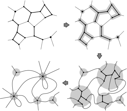
Figure 2: The procedure for shrinking the trees. Given a spanning forest $F$ over a graph $G$, we mark the components of the forest (here in bold) , and we shrink the trees with their leaves to single vertices respecting the ordering of the the border legs. Then we obtain $G/F$ (graph on the bottom left). The images on the right side represent intermediate steps, where we deform the graph and color in grey the region to be shrunk, to better visualize the procedure.

To keep track of the graph parameters all along this shrinking procedure, we assign to every effective vertex, obtained from a tree $T^{\prime}$ with $n$ vertices, an effective coupling $g_{n}=tg^{n}A^{\prime}_{h,n}$. These vertices have degree $hn+2$.

The generating function of graphs $G/F$, counted with the associated multiplicities, symmetries, and factor for the number of vertices, can thus be represented by the following one-Hermitian-matrix integral:

$$Z(t,g,N)=\frac{1}{N^{2}}\log\displaystyle{\frac{\int\mathrm{d}M\,e^{-N\,\mathop{\mathrm{Tr}}\nolimits V(M)}}{\int\mathrm{d}M\,e^{-N\mathop{\mathrm{Tr}}\nolimits\frac{1}{2}M^{2}}}}$$ (8)

where the potential is

$$V(z) =\frac{1}{2}z^{2}-\sum_{n\geq 1}g_{n}z^{hn+2}=\frac{1}{2}z^{2}(1-tA^{\prime}_{h}(gz^{h}))\,,$$ (9)

and we have called $A^{\prime}_{h}(x)$, the generating function $A^{\prime}_{h}(x)=\sum_{n\geq 1}A^{\prime}_{h,n}x^{n}$.

At this point we perform the integration over the angular degrees of freedom, and reduce to the eigenvalues basis, i.e., we write $M=U\,\Lambda\,U^{-1}$ and integrate over $U$. This produces the square of the Vandermonde determinant $\Delta(\{\lambda_{i}\})=\prod_{i<j}(\lambda_{i}-\lambda_{j})$ as Jacobian of this transformation:

$$Z(t,g,N)=\frac{1}{N^{2}}\log\displaystyle{\frac{\int\prod_{i=1}^{N}\,\mathrm{d}\lambda_{i}\,\Delta^{2}(\{\lambda_{i}\})\,e^{-N\sum_{i}V(\lambda_{i})}}{\int\prod_{i=1}^{N}\,\mathrm{d}\lambda_{i}\,\Delta^{2}(\{\lambda_{i}\})\,e^{-N\sum_{i}\frac{1}{2}\lambda_{i}^{2}}}}$$ (10)

and the eigenvalues are confined to the analyticity region of $A^{\prime}_{h}(x)$, namely $|x|<\frac{h^{h}}{(h+1)^{h+1}}$.

We have a single random matrix, which is convenient for the solution, but unfortunately the potential is not polynomial, this being in general a crucial obstacle. Nonetheless, there exists a suitable change of variables that leads to a polynomial potential, at the price of an additional Vandermonde–like term in the integrand. Indeed, calling $z=x(1-gx^{h})$, we have

$$z^{2}A^{\prime}_{h}(gz^{h})=\frac{x^{2}}{2}\left(\frac{2}{h+2}gx^{h}-(gx^{h})^{2}\right)\,.$$ (11)

so that, if we perform the change of variables $\lambda_{i}(x_{i})=x_{i}(1-gx_{i}^{h})$, we end up with the following expression:

$$\begin{split}Z(t,g,N)&=\frac{1}{N^{2}}\log\displaystyle{\frac{\int\prod_{i=1}^{N}\,\mathrm{d}x_{i}\,\Delta^{2}(\{x_{i}\})\,\hat{\Delta}_{g}(\{x_{i}\})\,e^{-N\sum_{i}\tilde{V}(x_{i})}}{\int\prod_{i=1}^{N}\,\mathrm{d}x_{i}\,\Delta^{2}(\{x_{i}\})\,e^{-N\sum_{i}\frac{1}{2}x_{i}^{2}}}}\\ &=\frac{1}{N^{2}}\log\displaystyle{\frac{\int\prod_{i=1}^{N}\,\mathrm{d}x_{i}\,\Delta^{2}(\{x_{i}\})\,\hat{\Delta}_{g}(\{x_{i}\})\,e^{-N\sum_{i}\tilde{V}(x_{i})}}{\int\prod_{i=1}^{N}\,\mathrm{d}x_{i}\,\Delta^{2}(\{x_{i}\})\,\hat{\Delta}_{g}(\{x_{i}\})e^{-N\sum_{i}\tilde{V}_{0}(x_{i})}}}\end{split}$$ (12)

where the potentials $\tilde{V}$ and $\tilde{V}_{0}$ are now both polynomial

$$\tilde{V}(x) =\frac{x^{2}}{2}\left(1-2g\left(1+\frac{t}{h+2}\right)x^{h}+g^{2}(1+t)x^{2h}\right)$$ (13)

$$\tilde{V}_{0}(x) =\frac{x^{2}}{2}\left(1-2gx^{h}+g^{2}x^{2h}\right)$$ (14)

and the new factor $\hat{\Delta}_{g}(\{x_{i}\})$ comes from the combination of the Jacobian and the change of the Vandermonde determinant in the new coordinates, and is

$$\hat{\Delta}_{g}(\{x_{i}\})=\prod_{i,j}(1-g(x_{i}^{h}+x_{i}^{h-1}x_{j}+\dots+x_{j}^{h}))\,.$$ (15)

3 Mapping to the O(n) Gravitational Loop Model at n = -​-2

3.1 Loop-dimer gas coupled to gravity

The O$(n)$ loop model has been proposed by Nienhuis [42] as a model with $n$-dimensional vector fields that, on cubic lattices, allowed for a simple combinatorial description in terms of self-avoiding cycles. The idea of universality in critical phenomena is that the critical exponents are related to the symmetry group of the system, including the target space of the elementary degrees of freedom, and in the Nienhuis model the underlying symmetry under (analytically-continued in $n$) O$(n)$ global rotations appears as a “weight factor $n$ per loop”, in a way similar to how a “weight $q$ per component” appears in the Fortuin–Kasteleyn formulation of the Potts Model, related to the (analytically-continued in $q$) permutational symmetry group $\mathfrak{S}_{q}$ for the Potts colours. We also remark that however there exist other spin models (in particular integrable vertex models) which can be mapped onto loop models of O$(n)$ and $q$-state Potts type and whose symmetry is different, see [43] for a systematic discussion.

Because of its combinatorial simplicity, its definition on arbitrary cubic graphs, and of its formulation well-adapted to the ‘model building’ of random matrices (see e.g. [14, sec. 2.5]), the O$(n)$ loop model had a prominent role in the development of statistical mechanics on random geometries, starting from the first seminal results [33, 34, 36], and is still considered a major realisation of the KPZ counterpart of the family of minimal CFT’s, and the most promising for a rigorous formalisation of this relation [44, 45, 26].

Therefore, and this will be crucial in this paper, once we have established the announced correspondence with the model of spanning forests, we have at disposal a large amount of established results and techniques.

Dimer models are another statistical-mechanics model which, besides a long tradition on ordinary regular graphs, is well adapted to the formalism of random planar graphs [46] (see also [14], pages 12-13 and 33). It is in fact one of the simplest cases of solvable such models, and the criticality has a simple pattern, which makes this model a candidate pedagogical example to illustrate the emerging features of Random Matrix theory.

In this section we consider a more general model, in which we have underlying graphs of fixed degree, $k=h+2$, and, as matter fields, both dimers and non-intersecting loops. The loops have fugacity $n$. This model, that we shall call loop-dimer gas model (we will write O$(n)$-loop–dimer gas model when we need to emphasize the value of $n$), has been studied by Kostov and Staudacher [36], as a continuation of the work of Kostov and Gaudin [33, 34] on the O$(n)$ model (with no dimers). As we will see, it is this model that is exactly related to spanning forests.

Such a hybrid model may appear baroque at a first look. However, at a deeper inspection, some justifications can be identified. First, the O$(n)$ loop model configurations are defined as a collection of cycles in the underlying graph which are vertex-disjoint. On a cubic graph, this coincides with cycles which are edge-disjoint. Edge-disjoint paths are in particular non-backtracking. Vertex-disjoint paths are also non-backtracking, unless they are cycles of length 2, in which case they form a structure isomorphic to a dimer. As, intrinsically, for cubic graphs and ‘long’ cycles, we do not see a difference between the constraints of being vertex- or edge-disjoint, it makes sense to consider the only possible local discrepancy – namely dimers – as included in the theory with an arbitrary weight.

A second, deeper reason is the fact that, as we have mentioned in the introduction (see [47] for a full account), on an arbitrary graph (even without averaging on the ensemble of planar graphs) there is a formulation of the spanning-forest partition function in terms of a Grassmann action which has a quadratic and a quartic term. The quadratic part is of the form ‘mass$\;+\;$Laplacian’, and the quartic part is associated to the marking of a dimer, i.e., the action is

$$\exp(S_{\rm forest})=\exp\bigg{(}\sum_{v}(t+\sum_{u\sim v}w_{uv})\bar{\psi}_{v}\psi_{v}-\sum_{(uv)}w_{uv}(\bar{\psi}_{v}\psi_{u}+\bar{\psi}_{u}\psi_{v})-t\sum_{(uv)}w_{uv}\bar{\psi}_{u}\psi_{u}\bar{\psi}_{v}\psi_{v}\bigg{)}$$ (16)

On the other side, following the combinatorial rules of Grassmann Algebra, we can investigate the meaning of an action

$$\exp(S)=\exp\bigg{(}\sum_{v}m_{v}\bar{\psi}_{v}\psi_{v}\bigg{)}\prod_{(uv)}(1-a_{uv}(\bar{\psi}_{v}\psi_{u}+\bar{\psi}_{u}\psi_{v})+b_{uv}\bar{\psi}_{u}\psi_{u}\bar{\psi}_{v}\psi_{v})$$ (17)

If we expand this polynomial, and keep only the term $\prod_{v}\bar{\psi}_{v}\psi_{v}$ (up to reordering), as appropriate for Grassmann–Berezin integration, we see that the contributions can be identified to configurations of edge-disjoint oriented cycles and dimers. Edges $(uv)$ in the cycles take a factor $a_{uv}$. Edges $(uv)$ covered by a dimer take a factor $b_{uv}$. Vertices $v$ not covered neither by a cycle, nor by a dimer, take a factor $m_{v}$. (Unoriented) cycles come with a ‘topological’ weight, which has a factor 2, accounting for the two possible orientations, and a factor $-1$, coming from the reordering of the Grassmann variables along the cycle. Thus, this is exactly a model of O$(-2)$ loops and dimers (this calculation is also sketched at the very end of [8]).

Now, taking care of sign factors coming from the reordering of fermions, we can easily exponentiate the edge factors in the action, to get

$$1-a_{uv}(\bar{\psi}_{v}\psi_{u}+\bar{\psi}_{u}\psi_{v})+b_{uv}\bar{\psi}_{u}\psi_{u}\bar{\psi}_{v}\psi_{v}=\exp\big{[}-a_{uv}(\bar{\psi}_{v}\psi_{u}+\bar{\psi}_{u}\psi_{v})+(b_{uv}+a_{uv}^{2})\bar{\psi}_{u}\psi_{u}\bar{\psi}_{v}\psi_{v}\big{]}$$ (18)

that is, exactly the spanning-forest action, provided we match the parameters as

$$\left\{\begin{array}[]{l}m_{v}=t+\sum_{u\sim v}w_{uv}\\ a_{uv}=w_{uv}\\ b_{uv}+a_{uv}^{2}=-tw_{uv}\end{array}\right.$$ (19)

If the underlying graph has uniform degree $k$, and uniform weights, this reduces to

$$\left\{\begin{array}[]{l}m=t+kw\\ a=w\\ b+a^{2}=-tw\end{array}\right.$$ (20)

that is, the partition function of loops and dimers coincides with the one for spanning forests, under the identification above, on the subspace of parameters

$$b=(k-1)a^{2}-am\,.$$ (21)

Later on, for conforming to the notation of Kostov and Staudacher (which in turns is fixed by the form of a certain functional equation), we will parametrise the weight of a loop–dimer configuration as

$$(-g_{1})^{V-V_{\rm L}-2d}n^{\ell}(4b_{0})^{(-V_{\rm L})}(g_{\rm D}g_{1}^{2})^{d}$$ (22)

where $V_{\rm L}$ is the number of vertices covered by loops, $\ell$ is the number of loops, and $d$ is the number of dimers. We will also set $g_{2}=-(k-1)g_{\rm D}g_{1}^{2}$. Thus we can identify

$$\left\{\begin{array}[]{l}m=-g_{1}\\ a=1/(4b_{0})\\ b=-g_{2}/(k-1)\end{array}\right.$$ (23)

and for spanning forests, requiring $n=-2$, we can reformulate the relation (21) above as

$$1+\frac{4b_{0}}{k-1}g_{1}+\left(\frac{4b_{0}}{k-1}\right)^{2}g_{2}=0\,.$$ (24)

Curiously enough, as we will see, the case of spanning forests with fugacity $-1$, which has a nice interpretation as trees with no internal activity, is also a special point in the theory of loops and dimers, as it corresponds to the point in the subspace of parameters in which dimers have zero fugacity. (We do not know if this is an accident or has a deeper reason.)

3.2 Reduction to a one-matrix theory

Let us now study the loop-dimer gas model on random planar graphs, with uniform degree $k=h+2$. As anticipated in (22), we weight configurations of dimers and loops by the factor

$$(-g_{1})^{V-V_{\rm L}}n^{\ell}(4b_{0})^{-V_{\rm L}}g_{\rm D}^{d}$$

where $V$ is the total number of vertices, $\ell$ is the number of loops, $d$ is the number of dimers, and $V_{\rm L}$ is the number of vertices covered by loops.

Let us start by assuming that $n$ is a non-negative integer (we will perform an analytic continuation afterwards). As customary for the construction of Random Matrix theories associated to statistical-mechanics models, following the rules of Wick theorem (see e.g. [14, sect. 2]), we shall introduce matrices $B$ for unoccupied edges, $D$ for dimers, and $\{A_{c}\}_{c=1,\dots,n}$ for marked edges, coloured in one of $n$ colours (this reproduces the factor $n^{\ell}$).

As a result, this model is described by the following matrix integral:

$$Z^{l-d}_{N}(g_{1},b_{0},\gamma) =\log\displaystyle{\frac{\int\mathrm{d}A_{1}\dots\mathrm{d}A_{n}\mathrm{d}B\mathrm{d}D\,e^{-N\mathop{\mathrm{Tr}}\nolimits W(A_{1},...,A_{n},B,D)}}{\int\mathrm{d}A_{1}\dots\mathrm{d}A_{n}\mathrm{d}B\mathrm{d}D\,e^{-N\mathop{\mathrm{Tr}}\nolimits W_{0}(A_{1},...,A_{n},B,D)}}}$$ (25)

$$W(A_{1},...,A_{n},B,D) =\frac{1}{2}B^{2}+\frac{1}{2}\sum^{n}_{c=1}A_{c}^{2}+\frac{1}{2}D^{2}+\frac{g_{1}}{k}B^{k}+\sqrt{g_{\rm D}}g_{1}B^{k-1}D+$$

$$\quad-\frac{1}{8b_{0}}\sum_{c=1}^{n}\sum_{h^{\prime}=0}^{h}B^{h^{\prime}}A_{c}B^{h-h^{\prime}}A_{c}$$

$$W_{0}(A_{1},...,A_{n},B,D) =\frac{1}{2}B^{2}+\frac{1}{2}\sum^{n}_{c=1}A_{c}^{2}+\frac{1}{2}D^{2}\,.$$

We have made the choice of having the quadratic part trivial. As a result, in the model construction, we have weights associated to “vertices” of interaction, and no weights associated to edges. A monomial of the form $-\frac{1}{|\mathop{\mathrm{Aut}}\nolimits|}g\prod_{i}M_{c(i)}$ corresponds to a vertex with edge-colour content $\{c(i)\}$, weighted with a factor $g$. As a result, it is easily recognised that, as desired, vertices of the graph not in any dimer or loop, associated to the term $g_{1}/kB^{k}$, come with a weight $-g_{1}$. Vertices in a loop, associated to the last term of the potential, come with weight $1/(4b_{0})$, and each of the two vertices of a dimer come with weight $-\sqrt{g_{\rm D}}g_{1}$.

If we shrink dimers to points, those can be seen as vertices of degree $2k-2$ with a coupling $g_{\rm D}g_{1}^{2}$. The algebraic counterpart of this is the Gaussian integral over matrix $D$. As a result, the action becomes

$$W=\frac{1}{2}B^{2}+\frac{1}{2}\sum^{n}_{c=1}A_{c}^{2}+\frac{g_{1}}{k}B^{k}+\frac{g_{2}}{2k-2}B^{2k-2}-\frac{1}{8b_{0}}\sum_{c=1}^{n}\sum_{h^{\prime}=0}^{h}B^{h^{\prime}}A_{c}B^{h-h^{\prime}}A_{c}\,,$$ (26)

where we have introduced $g_{2}:=-(k-1)g_{\rm D}g_{1}^{2}$ (again, with the aim of exposing a $1/|\mathop{\mathrm{Aut}}\nolimits|$ factor). After passing to the eigenvalue basis for matrix $B$

$$B\longrightarrow U\mbox{diag}(x_{1},\dots,x_{N})U^{-1},\qquad A_{c}\longrightarrow UA_{c}U^{-1}\,,$$ (27)

the part of the action depending on the matrices $A_{c}$ reads

$$\frac{1}{2}\sum_{ij}(A_{c})_{ij}(A_{c})_{ji}\left(1-\frac{1}{4b_{0}}(x_{i}^{h}+x_{i}^{h-1}x_{j}+\dots+x_{j}^{h})\right)\,,$$ (28)

and if we integrate out the matrices $A_{c}$ we end up with the following one-matrix integral:

$$Z^{l-d}_{N}(g_{1},g_{2},b_{0})=\log\displaystyle{\frac{\int\prod_{i=1}^{N}\,\mathrm{d}x_{i}\,\Delta^{2}(\{x_{i}\})\,\left(\hat{\Delta}_{1/(4b_{0})}(\{x_{i}\})\right)^{-n/2}\,e^{-N\sum_{i}V(x_{i})}}{\int\prod_{i=1}^{N}\,\mathrm{d}x_{i}\,\Delta^{2}(\{x_{i}\})\,e^{-N/2\sum_{i}x_{i}^{2}}}}\,.$$ (29)

where $\hat{\Delta}$ is the same quantity defined in (15), and

$$V(x)=\frac{x^{2}}{2}+\frac{g_{1}}{k}x^{k}+\frac{g_{2}}{2k-2}x^{2k-2}\,.$$ (30)

Now we compare the partition functions for spanning forests (12) and for the O$(n)$ loop-dimer gas (29). These are identical if we set $n=-2$ and identify the parameters of the two models in the following way:

$$\left\{\begin{array}[]{l}\frac{1}{4b_{0}}=g\\ g_{1}=-g(k+t)\\ g_{2}=(k-1)g^{2}(1+t)\end{array}\right.\,.$$ (31)

Note that this identification corrects the derivation in [32], and will allow us to draw conclusions on the critical behaviour of spanning forests using the available results for the O$(n)$ model. Also note that, not surprisingly, this substitution satisfies the condition (24). That is, if we substitute (31) into $1+\frac{4b_{0}}{k-1}g_{1}+\big{(}\frac{4b_{0}}{k-1}\big{)}^{2}g_{2}$ we get $1-\frac{k+t}{k-1}+\frac{1+t}{k-1}=0$. In turns, the procedure of this section, of averaging over a certain statistical ensemble of (planar) graphs with fixed degree $k$, has obviously implemented the same condition that holds separately for each and every graph of degree $k$.

4 Analysis of the Random Matrix Model at genus zero

In this section we will discuss the critical behavior of spanning forests on random planar graphs by studying the large-$N$ limit of the matrix integral (8). We refer the reader to the reviews [13, 14, 15] for background material on techniques for matrix models. We will try to give a self–consistent presentation, mainly following [13] and adapting it to our case. An ingredient of our problem, with respect to the (nowadays standard) treatments presented in the forementioned reviews, is that we have to trade one or the other complication: either we have an extra factor $\hat{\Delta}$ beside the customary Vandermonde factors (in variables $x$, w.r.t. notations of Section 2), or we deal with a potential of the one-matrix model which is not polynomial (in variables $z$). We adopt this second approach. As will be discussed, the standard formulas for a polynomial potential go through with little modification, but obtaining explicit solutions poses new technical challenges.

4.1 Saddle-point equation

To facilitate the singularity analysis it is convenient to perform the change of variables $M\to g^{-1/h}M$ which, apart from an irrelevant prefactor $g^{-N^{2}/h}$, leaves us with the following matrix integral replacing the numerator of (8):

$$\int\mathrm{d}M\,\exp\left(-\frac{N}{v}\,\mathop{\mathrm{Tr}}\nolimits W(M)\right)\,,$$ (32)

where $W$ coincides with $V$ with $g$ set to one:

$$W(z) =\frac{1}{2}z^{2}-t\sum_{n\geq 1}A^{\prime}_{h,n}z^{hn+2}\,,$$ (33)

and for easiness of notation we introduced

$$v=g^{2/h}\,.$$ (34)

We recall that the parameter $h+2$ is the degree of the graph, and that the series in $n$, $A^{\prime}_{h,n}$, has region of convergence

$$|z|<r_{h}\equiv\frac{h}{(h+1)^{(h+1)/h}}\,.$$ (35)

The potential can be analytically continued to a larger region in the complex plane, as will be discussed below for the first few values of $h$.

In the eigenvalue basis, the integrand is $e^{-N^{2}S(\{\lambda_{i}\})}$, with the action

$$S(\{\lambda_{i}\})=\frac{1}{v}\frac{1}{N}\sum_{i=1}^{N}W(\lambda_{i})-\frac{1}{N^{2}}\sum_{1\leq i\neq j\leq N}\log|\lambda_{i}-\lambda_{j}|\,,$$ (36)

and the saddle-point equation $\partial_{\lambda_{\ell}}S=0$ results in

$$\frac{1}{v}W^{\prime}(\lambda_{\ell})=\frac{2}{N}\sum_{i(\neq\ell)}\frac{1}{\lambda_{\ell}-\lambda_{i}}\,.$$ (37)

In the large-$N$ limit the action (36) becomes a functional of the spectral density

$$\rho(\lambda)=\lim_{N\to\infty}\frac{1}{N}\sum_{i=1}^{N}\delta(\lambda-\lambda_{i})\,,$$ (38)

and reads

$$S(\lambda)=\frac{1}{v}\int\,\mathrm{d}\lambda\rho(\lambda)W(\lambda)-\fint\,\mathrm{d}\lambda\,\mathrm{d}\lambda^{\prime}\rho(\lambda)\rho(\lambda^{\prime})\log|\lambda-\lambda^{\prime}|\,,$$ (39)

where the double integral in the second summand is regularized by its Cauchy principal value. It is understood that the support of $\rho$ shall be contained within the forementioned domain of analyticity of $W$. In the planar limit the saddle-point equation becomes the following integral equation

$$\frac{1}{v}W^{\prime}(\lambda) =2\fint\,\mathrm{d}\lambda^{\prime}\frac{\rho(\lambda^{\prime})}{\lambda-\lambda^{\prime}}\,,\quad\lambda\in\text{supp}(\rho)\,,$$ (40)

which computes the extrema of the functional $S(\rho)$. This equation has to be solved together with the normalization condition

$$\int\,\mathrm{d}\lambda\,\rho(\lambda)=1\,.$$ (41)

Given a solution of the saddle-point and normalization equations, the generating function of spanning forests for random planar graphs is then given by

$$\lim_{N\to\infty}Z(t,g,N)=S_{0}(\rho_{0})-S(\rho)\,,$$ (42)

where $Z(t,g,N)$ was defined in (8). The action $S_{0}$ is given by (39) with $W(\lambda)/v$ replaced by $V_{0}(\lambda)=\lambda^{2}/2$, and thus $\rho_{0}$ is given by the celebrated Wigner semicircle formula, $S_{0}(\rho_{0})$ is just a constant, which can be ignored as far as the singularity analysis is concerned.

4.2 Solution of the saddle-point equation

As standard, the singular integral equation representing the saddle point is solved by rewriting it as a Riemann–Hilbert problem for the resolvent $\omega$. Introducing

$$\omega(z)=\frac{1}{N}\sum_{i=1}^{N}\frac{1}{z-\lambda_{i}}\,,$$ (43)

few lines of calculation, starting from the saddle-point equation, show that in the large $N$ limit $\omega$ satisfies

$$\omega^{2}(z)=\frac{1}{v}W^{\prime}(z)\omega(z)-\frac{1}{4v^{2}}P(z)\,,\quad P(z)=4v\int\,\mathrm{d}\lambda\rho(\lambda)\frac{W^{\prime}(z)-W^{\prime}(\lambda)}{z-\lambda}\,.$$ (44)

The quantity $P(z)$ is yet to be determined. As apparent from its definition, it is guaranteed to be analytic only in the domain where $W(z)$ is. At large $N$, the relation between $\omega$ and $\rho$ is

$$\omega(z) =\int\,\mathrm{d}\lambda\frac{\rho(\lambda)}{z-\lambda}\,,$$ (45)

which shows that $\omega$ is an analytic function in $\mathbb{C}\setminus\text{supp}(\rho)$, this despite $W$ being possibly not analytic in all $\mathbb{C}$ (as is the case here). Furthermore, Eq. (41) implies the asymptotic behavior

$$\omega(z)\sim\frac{1}{z}\,,\quad z\to\infty\,.$$ (46)

Define $\omega^{\pm}(\lambda)=\omega(\lambda\pm i0)$ as the values right above and below the support of $\rho$. One has the following equations

$$\left\{\begin{array}[]{l}\omega^{-}(\lambda)-\omega^{+}(\lambda)=2\pi i\rho(\lambda)\,;\\ \rule{0.0pt}{13.0pt}\omega^{-}(\lambda)+\omega^{+}(\lambda)=\frac{1}{v}W^{\prime}(\lambda)\,;\end{array}\right. \lambda\in\text{supp}(\rho)\,.$$ (49)

The latter corresponds to the aforementioned Riemann–Hilbert problem. Roughly speaking, its solvability requires that $W^{\prime}$ is continuous on any open set within $\text{supp}(\rho)$, a condition certainly met in our case. (See e.g. [48] for a more precise treatment.)

We now discuss the solution of the second of the equations above. We make the customary one–cut assumption that the support of $\rho$ consists of a single segment, that we parametrise as $[a_{1},a_{2}]$. This means that the problem has to be solved with the further requirement that $\rho>0$ on $[a_{1},a_{2}]$, where $a_{1},a_{2}$ will be determined as functions of the parameters in the problem. If positivity fails for some parameter range, then the assumption is invalidated, and, most probably, multiple cuts need to be considered. Let us define

$$\sigma(z)=(z-a_{1})(z-a_{2})\,,$$ (50)

we can write

$$\omega(z)=\frac{1}{2v}\left(W^{\prime}(z)-\sqrt{W^{\prime}(z)^{2}-4P(z)}\right)=\frac{1}{2v}\left(W^{\prime}(z)-M(z)\sqrt{\sigma(z)}\right)\,,$$ (51)

where $M$ is analytic in some open set containing the interval $[a_{1},a_{2}]$. These prescriptions are sufficient to determine $M$ and $\omega$ uniquely. We report here the derivation of [15], while paying attention to analyticity properties, which are slightly different in the case at hand. We recall that $\mathbb{C}\setminus[a_{1},a_{2}]$ is the domain of analyticity of $\omega/\sqrt{\sigma}$, and consider in it a point $z$ and a cycle $C_{z}$ around $z$. Further, we denote by $C_{[a_{1},a_{2}]}$ a cycle around $[a_{1},a_{2}]$ which does not enclose $z$, and assume that it is contained in the domain of analyticity of $W$. Then, one has

$$\frac{\omega(z)}{\sqrt{\sigma(z)}}=\frac{1}{2\pi i}\oint_{C_{z}}\frac{\,\mathrm{d}w}{w-z}\frac{\omega(w)}{\sqrt{\sigma(w)}}=-\frac{1}{2\pi i}\oint_{C_{[a_{1},a_{2}]}}\frac{\,\mathrm{d}w}{w-z}\frac{\omega(w)}{\sqrt{\sigma(w)}}$$ (52)

$$=-\frac{1}{2\pi i}\frac{1}{2v}\oint_{C_{[a_{1},a_{2}]}}\frac{\,\mathrm{d}w}{w-z}\frac{W^{\prime}(w)}{\sqrt{\sigma(w)}}=\frac{1}{2\pi i}\frac{1}{v}\int_{a_{1}}^{a_{2}}\frac{\,\mathrm{d}\mu}{\mu-z}\frac{W^{\prime}(\mu)}{\sqrt{\sigma(\mu)}}\,.$$ (53)

Correspondingly, the formula for the spectral density is

$$\rho(\lambda)=\frac{1}{2\pi^{2}v}\sqrt{-\sigma(\lambda)}\fint_{a_{1}}^{a_{2}}\frac{\,\mathrm{d}\mu}{\mu-\lambda}\frac{W^{\prime}(\mu)}{\sqrt{-\sigma(\mu)}}\,.$$ (54)

The spectral edges of the support are chosen to ensure the correct large-$z$ behavior of $\omega$, equation (46), and are determined by the following equations:

$$\int_{a_{1}}^{a_{2}}\,\mathrm{d}\mu\frac{W^{\prime}(\mu)}{\sqrt{-\sigma(\mu)}} =0\,,$$ (55a)

$$\int_{a_{1}}^{a_{2}}\,\mathrm{d}\mu\frac{\mu W^{\prime}(\mu)}{\sqrt{-\sigma(\mu)}} =2\pi v\,.$$ (55b)

The first one is a necessary condition for the solvability of the Riemann–Hilbert problem, while the second one ensures normalization of $\rho$. By passing to contour integrals around the support, and changing variables via the Joukowski map,

$$\mu =S+z+\frac{R}{z}\,, S =\frac{a_{1}+a_{2}}{2}\,, R =\left(\frac{a_{1}-a_{2}}{4}\right)^{2}\,,$$ (56)

one can rewrite these conditions as

$$\oint\frac{\,\mathrm{d}z}{2\pi iz}W^{\prime}(\mu(z)) =0\,,$$ (57a)

$$\oint\frac{\,\mathrm{d}z}{2\pi i}W^{\prime}(\mu(z)) =v\,.$$ (57b)

We now specify these formulas to our potential (33). Its derivative is

$$W^{\prime}(z) =z-t\sum_{n\geq 1}A_{h,n}z^{hn+1}\,,$$ (58)

where the $A_{h,n}$ numbers are Fuss–Catalan numbers:

$$A_{h,n}=\frac{((h+1)n)!}{n!(hn+1)!}\,.$$ (59)

The conditions on $a_{1}$, $a_{2}$, or equivalently $R$, $S$ (through (56)), then read as follows:

$$S =t\,\sum_{n\geq 1}\sum_{q\geq 0}A_{h,n}\frac{(hn+1)!}{(hn-q+1)!^{2}(hn-2q+1)}R^{hn-q+1}S^{2q-hn-1}\,,$$ (60a)

$$v =R-t\sum_{n\geq 1}\sum_{q\geq 0}A_{h,n}\frac{(hn+1)!}{(hn-q+1)!(hn-q)!(hn-2q)!}R^{hn-q+1}S^{2q-hn}\,.$$ (60b)

These equations coincide with those appearing in [35, Thm 3.1] (they use $z$ and $u$ in place of $v$ and $t$). Remarkably, they were derived with a purely combinatorial method, quite different from the one presented. The fact that both approaches lead to the same equations is rooted in previous work [26] on which [35] is based, and the connection between combinatorial methods and matrix models [49, 14].

4.3 Saddle-point equation for the O(n = -​-2) model

We present now the reformulation of the saddle-point equation from the point of view of the O$(n)$ model. As already mentioned, the resulting potential will be polynomial, at the expenses of a more complicated form of the equation. In order to make contact with the formulas of Section 3.1, we will work here with the original $V$ which contains $g$ explicitly. We remind the reader that the connection with the O$(n)$ model emerges upon the change of variables $z\to x(z)$, whose inverse is $f(x):=z(x)=x(1-gx^{h})$ (note that $z^{\prime}(x)=1-g(h+1)x^{h}$), and that this leads to a polynomial potential:

$$\tilde{V}(x) =V(x(z))=\frac{x^{2}}{2}+\frac{g_{1}}{h+2}x^{h+2}+\frac{g_{2}}{2h+2}x^{2h+2}\,,$$ (61)

$$\frac{d\tilde{V}(x)}{dx} =\frac{dV(z)}{dz}\frac{dz(x)}{dx}=V^{\prime}(f(x))f^{\prime}(x)=x+g_{1}x^{h+1}+g_{2}x^{2h+1}\,.$$ (62)

We define $\tilde{\rho}$ as the distribution density in the new variable

$$\tilde{\rho}(y):=f^{\prime}(y)\rho(f(y))\,,$$ (63)

the factor $f^{\prime}(y)$ arises from the Jacobian of the transformation, i.e.

$$\,\mathrm{d}y\tilde{\rho}(y) =\,\mathrm{d}\mu\rho(\mu)\,, \mu =f(y)\,.$$ (64)

In terms of $\tilde{\rho}$, the large-$N$ action is

$$\tilde{S}(\tilde{\rho})=\int\,\mathrm{d}x\tilde{\rho}(x)\tilde{V}(x)-\fint\,\mathrm{d}x\,\mathrm{d}y\tilde{\rho}(x)\tilde{\rho}(y)\log|f(x)-f(y)|\,,$$ (65)

and the saddle-point equation becomes:

$$x+g_{1}x^{h+1}+g_{2}x^{2h+1}=2f^{\prime}(x)\fint\,\mathrm{d}y\frac{\tilde{\rho}(y)}{f(x)-f(y)}\,.$$ (66)

Noting that $(f(x)-f(y))/(x-y)$ is a polynomial in $x$ and $y$, and calling $\xi_{1}^{(h)}(y)$, …, $\xi_{h}^{(h)}(y)$ its roots as a polynomial in $x$, it is in fact the case that

$$\frac{1}{x-y}+\sum_{j=1}^{h}\frac{1}{x-\xi_{j}^{(h)}(y)}=\frac{f^{\prime}(x)}{f(x)-f(y)}$$ (67)

so that (66) can be reformulated as

$$x+g_{1}x^{h+1}+g_{2}x^{2h+1}=2\fint\,\mathrm{d}y\tilde{\rho}(y)\bigg{(}\frac{1}{x-y}+\sum_{j=1}^{h}\frac{1}{x-\xi_{j}^{(h)}(y)}\bigg{)}\,.$$ (68)

It is easy to see that, for small $g$, these roots converge to the roots of unity, multiplied by $g^{-1/h}$, for example, at $h=1$ and 2 we have

$$h=1:\quad \xi_{1}^{(1)}(y) =(g^{-1}-y)$$ (69)

$$h=2:\quad \xi_{1,2}^{(2)}(y) =-\frac{y}{2}\pm\sqrt{g^{-1}-{\textstyle\frac{3}{4}}y^{2}}$$ (70)

and thus, for $x$ and $y$ small w.r.t. such a quantity, the denominators $x-\xi_{j}^{(h)}(y)$ do not vanish. Let $b$ be the largest value in the support of $\tilde{\rho}$. It will turn out that we have an interesting behavior when $b$ is large enough for one of these denominators to vanish. If we imagine to increase the value of $b$, this is first possible when both $x$ and $y$ are near $b$, i.e. when $\lim_{x,y\to b}\frac{f(x)-f(y)}{x-y}=\lim_{x\to b}f^{\prime}(x)=0$, which corresponds to the condition $(h+1)gb^{h}=1$. In terms of the original variable $\lambda$, this singularity occurs when the right spectral edge reaches the critical radius of $W$.

On the other hand, Eq. (66) can also be rewritten as

$$x+g_{1}x^{h+1}+g_{2}x^{2h+1}=2f^{\prime}(x)\fint\,\mathrm{d}y\frac{\tilde{\rho}(y)}{f^{\prime}(y)}\left(\frac{1}{x-y}+\sum_{i=1}^{h}\frac{1}{\xi_{i}^{h}(x)-y}\right)\,.$$ (71)

In terms of the resolvent

$$\tilde{\omega}(z)=f^{\prime}(x)\int\,\mathrm{d}y\frac{\tilde{\rho}(y)}{f^{\prime}(y)}\frac{1}{z-y}\,,$$ (72)

this equation reads as:

$$x+g_{1}x^{h+1}+g_{2}x^{2h+1}=\tilde{\omega}^{+}(x)+\tilde{\omega}^{-}(x)+2\sum_{i=1}^{h}\tilde{\omega}(\xi^{h}_{i}(x))\,,\quad x\in\text{supp}(\tilde{\rho})$$ (73)

since $f^{\prime}(x)$ is a polynomial and therefore continuous, and $\xi_{i}(x)$ are outside the support of $\tilde{\rho}$. We remark that similar equations appear also in other statistical mechanical problems, see e.g. [50, 51, 52], and general techniques for dealing with these equations have been developed in [45].

To the best of our knowledge the critical behavior of the O$(n)$ loop gas on a graph of arbitrary degree, as the one appearing in section 3.2, has not been discussed in the literature. The only explicit results relevant for us are for the case $h=1$, and are discussed in several works, among which the seminal paper [36]. The method employed in [36] is to start from our equation (66) and map it back to the standard singular integral equation appearing in (40), at the expenses of a non polynomial potential. The singular equation is then solved along the lines discussed above. The authors of [36] discussed however only isolated critical points corresponding to $t=0$ and $t=-1$ in our notation, and not the presence of a massless phase, the quantum gravity counterpart of the Berker–Kadanoff phase, which to our knowledge has been found only much later, in [35]. In section 4.7 we will present a self–contained discussion of the solution for $h=1$, which agrees with the one presented by [36] at the specific values of the couplings mentioned above.

Interestingly, the criticality of one-matrix models with non-polynomial potentials has been investigated in recent work [53], whose findings are possibly of relevance also for the model at hand.

4.4 Singular behavior of the partition function

Knowledge of the spectral density determines the partition function and all the correlators of a matrix model. Recall Eq. (42) and the formula:

$$\left<\mathop{\mathrm{Tr}}\nolimits f_{1}(M)\cdots\mathop{\mathrm{Tr}}\nolimits f_{n}(M)\right>=N^{n}\int\,\mathrm{d}\lambda_{1}\cdots\,\mathrm{d}\lambda_{n}f_{1}(\lambda_{1})\cdots f_{n}(\lambda_{n})\left<\rho(\lambda_{1})\cdots\rho(\lambda_{n})\right>\,.$$ (74)

Here $\left<\cdot\right>$ stands for the average w.r.t the measure defined by (32). Further, in one-matrix models with a connected spectral support, the critical behavior is determined only by the spectral edges, and this result is universal in the sense that it holds for any potential [13]. For the reader’s convenience, we re-derive this result in this section. The reason for this universality can be traced back to equation (49) and the way $v$ enters in it. Indeed the function

$$\Omega(z)=\frac{\partial(v\omega(z))}{\partial v}\,,$$ (75)

satisfies

$$\Omega^{+}(\lambda)+\Omega^{-}(\lambda)=0\,,$$ (76)

independently of $W$. From the behavior $\Omega(z)\sim z^{-1}$ as $z\to\infty$, and the one-cut assumption one obtains $\Omega(z)=1/\sqrt{\sigma(z)}$, and therefore

$$\frac{\partial(v\rho(\lambda))}{\partial v}=\frac{1}{\pi}\frac{1}{\sqrt{-\sigma(\lambda)}}\,.$$ (77)

One then notices that in the large-$N$ limit the derivative of $Z$ is

$$v^{3}\frac{\partial Z}{\partial v}=vN\left<\mathop{\mathrm{Tr}}\nolimits W\right>\sim N^{2}\int_{a_{1}}^{a_{2}}\,\mathrm{d}\lambda\,(v\rho(\lambda))\,W(\lambda)\,,$$ (78)

and therefore

$$\frac{\partial^{2}}{\partial v^{2}}\left(v^{3}\frac{\partial Z}{\partial v}\right) \sim\frac{N^{2}}{4\pi i}\Bigg{(}\frac{\partial a_{1}}{\partial v}\oint\,\mathrm{d}\lambda\frac{W(\lambda)}{(\lambda-a_{1})^{\frac{3}{2}}(\lambda-a_{2})^{\frac{1}{2}}}+\frac{\partial a_{2}}{\partial v}\oint\,\mathrm{d}\lambda\frac{W(\lambda)}{(\lambda-a_{2})^{\frac{3}{2}}(\lambda-a_{1})^{\frac{1}{2}}}\Bigg{)}$$

$$=N^{2}v\frac{\partial}{\partial v}\log(16R)\,,$$ (79)

where the second equality follows from integrating by parts the constraints (55). Furthermore, near to the critical point, as $\epsilon=1-v/v_{c}\to 0$, after replacing powers of $v$ with $v_{c}$ and integrating, one obtains

$$Z^{\prime\prime}\sim\frac{N^{2}}{v_{c}^{2}}\log(16R)\,.$$ (80)

Therefore the singular behavior of $Z$ can be obtained just by knowing the behavior of $R$ close to a critical point, and this can be inferred from equations (60). By the transfer principle, knowing the leading dependence of $Z$ in $\epsilon$ dictates the asymptotic behavior of $Z_{n}$, where $Z=\sum_{n\geq 1}Z_{n}g^{n}$:

$$Z=\epsilon^{-\alpha}\log^{\beta}(\epsilon)\Rightarrow Z_{n}=g_{c}^{-n}n^{\alpha-1}\log^{\beta}(n)\left(\frac{1}{\Gamma(\alpha)}+\frac{\beta}{\log(n)}\frac{\,\mathrm{d}}{\,\mathrm{d}s}\frac{1}{\Gamma(s)}\Big{|}_{s=\alpha}+\dots\right)\,.$$ (81)

For a proof of this result, see [54, Thm. 6.2]. From the asymptotic behavior of $Z_{n}$ we define the critical exponents

$$Z_{n}\sim n^{\gamma-3}\log(n)^{\gamma^{\prime}}\,,$$ (82)

where, at least when $\gamma^{\prime}=0$, $\gamma$ is interpreted as the string susceptibility exponent and is related to the central charge of the model coupled to gravity by the KPZ formula (84) [13].

Let us pause for a moment our calculations, and make a digression on the subtleties of using KPZ here. The original KPZ formula [17] reads

$$\gamma=2-\frac{1}{12}\left(25-c+\sqrt{(1-c)(25-c)}\right)\,.$$ (83)

From this, and $\gamma=-1$, it is easily recovered the well-known value $c=-2$ for the central charge of uniform spanning trees in dimension two. The situation is in fact more complex, although the conclusions are unchanged. The formula above holds, in principle, only for unitary CFTs. In non-unitary theories, the formula is modified into

$$\begin{split}\gamma&=2-\frac{2}{24+c_{\rm eff}-c}\left(25-c+\sqrt{(1-c_{\rm eff})(25-c)}\right)\\ &=2-\frac{1}{12(1-h_{\rm min})}\left(25-c+\sqrt{(1+24h_{\rm min}-c)(25-c)}\right)\,,\end{split}$$ (84)

where $c_{\rm eff}=c-24h_{\rm min}$ is the ‘effective’ central charge, and $h_{\rm min}$ is the lowest conformal dimension in the theory [46, 55]. In the CFT for spanning trees, there is a single field with negative dimension, $h=-1/8$ (see [56, 57]), so that we shall obtain $\gamma=0$. However, this field is associated to a twist operator for the boundary conditions, which is absent from the setting in which we constructed our theory, so that the formula with $h_{\rm min}=0$ shall be used, and $\gamma=-1$ is obtained accordingly. We conjecture that, in genus 1, there might be a way of constructing a model in which the twist operator is present (besides the obvious generalisation of the treatment here to higher genus, in which it would be absent), but we do not investigate this aspect here.

To the best of our knowledge, the exponent $\gamma^{\prime}$ has not been discussed in the context of Liouville theory coupled to the present CFT. Nonetheless, logarithmic corrections in lattice discretizations of $c=1$ CFTs are well known, both for flat [58] and fluctuating graphs [59], and their interpretation here may also be accessible at the light of [8].

Below we will discuss the critical behaviour in several cases. Some of these cases were already studied in [35], and for these we re-derive and extend their results from a random matrix perspective. The generating function for spanning forests $F(z,u)$ considered in [35] is expressed in terms of $R,S$ and, since the definition of $F$ lacks the factor $|\mathop{\mathrm{Aut}}\nolimits(G/F)|$ present in (2), it is expected to have the same singular behavior as $\partial Z/\partial g$. We remark that the random matrix derivation provides a direct connection between the singularity of $Z$ and that of $R$ via (80) (in particular, there is no need of usig $S$, even in the case of odd degree), and this fact, not used in [35], simplifies the singularity analysis.

Let us conclude this section with a comment on the case of spanning trees, which is arguably the simplest case. As is apparent from formula (2), spanning trees emerge as

$$Z_{\text{tree}}(g,N)=\lim_{t\to 0}\frac{\partial}{\partial t}Z(t,g,N)=-\frac{1}{N}\sum_{n\geq 1}g^{n}A^{\prime}_{h,n}\left<M^{hn+2}\right>_{0}\,,$$ (85)

where $\left<\cdot\right>_{0}$ is the average w.r.t. the Gaussian measure. In the large $N$ limit the result is well known [14] and given by the Catalan numbers:

$$\lim_{N\to\infty}\frac{1}{N}\left<M^{r}\right>_{0}=\begin{cases}\frac{1}{p+1}\binom{2p}{p}&\text{if }r=2p\,,\\ 0&\text{otherwise,}\end{cases}$$ (86)

(and recall that $A^{\prime}_{h,n}$ is itself a Fuss–Catalan number). One then recovers the expression for the generating function of spanning trees on random planar graphs exactly from the matrix integral (see [32] for further details and references). Here we just recall that the asymptotics $Z_{n}\sim g_{c}^{-n}n^{-4}$, with $g_{c}$ determined by the radius of convergence of the series,

$$g_{c}=2^{-h}\frac{h^{h}}{(h+1)^{(h+1)}}\,.$$ (87)

This behavior corresponds via the KPZ formula to $c=-2$, the known central charge for the problem on flat lattices (see although the caveat mentioned a few lines above).

4.5 The case of quartic graphs

We start by discussing the case of quartic graphs, i.e. $4$-regular graphs. Since the potential is even, the support will be of the form $[-a,a]$, and therefore $S=0$, $R=a^{2}/4$. Equations (60) then reduce to

$$g=R-t\Phi(R)\,, \Phi(R) =R\left({}_{2}F_{1}(\tfrac{1}{3},\tfrac{2}{3};2;27R)-1\right)\,.$$ (88)

Note that the radius of convergence of $\Phi$ is

$$\tau=\frac{r_{2}^{2}}{4}=\frac{1}{27}\,,$$ (89)

where $r_{2}$ is the radius of convergence of $W$. The singularity analysis of this implicit equation for $t\geq-1$ was carried out in [35, Sec. 8]. Here we will recall the main steps, and extend the analysis to all values of $t$. (See [54] for a reference on singularity analysis. The words singular, non–regular and non–analytic are used as synonyms.) The central result is an instance of the implicit function theorem, which asserts that given a function $\Omega(R)$ analytic at $R_{0}$, and $\Omega^{\prime}(R_{0})\neq 0$, there exists an inverse $R(g)$, such that $\Omega(R)=g$, and $R(g)$ is analytic in a neighbourhood of $g_{0}=\Omega(R_{0})$. The proof is well known and relies on analyticity of $\Omega$ at $R_{0}$ to expand it in Taylor series. There are thus two competing sources for the failure of analyticity of an implicit function: (1) $\Omega$ is singular at $R$; (2) $\Omega$ is regular at $R$ but $\Omega^{\prime}(R)=0$. If $R(g)$ is analytic at the origin, the singular behavior of $R$ and the exponential growth of its coefficients are dictated by $\rho$, the radius of the nearest singular point.

In our case $\Omega(R)=R-t\,\Phi(R)$, and $\Omega^{\prime}(R)=1-t\,\Phi^{\prime}(R)$. We note that our $\Omega$ can be analytically continued to $\mathbb{C}\setminus[\tau,\infty)$. Our goal being the singularity analysis for arbitrary real $t$, we will not restrict the values of $R,g$ to their initial range of definition, namely $R\in(0,\tau),g>0$, but consider them as complex parameters, and postpone the interpretation of the results, and possible ‘physical restrictions’, to the end of the calculation.

In light of the discussion above, the two kinds of singular points are:

1. triples $(t,R_{1},g_{1})$ such that $R_{1}=\tau$ and $g_{1}(t)=\tau-t\,\Phi(\tau)=\frac{1}{27}(t+1)-\frac{\sqrt{3}}{12\pi}t$;

2. triples $(t,R_{2},g_{2})$ such that $t^{-1}=\Phi^{\prime}(R_{2})$ and $g_{2}(t(R_{2}))=R_{2}-\frac{\Phi(R_{2})}{\Phi^{\prime}(R_{2})}$ (as we substitute $t^{-1}=\Phi^{\prime}(R_{2})$ in (88)).

Once we fix a value of $t$, among all triples $(t,R,g)$ realising one of the two mechanisms above, we have to identify the one with smallest value of $|g|$.

For this identification, it is useful to observe that $\Phi^{\prime}(R)$ is an increasing function of $R$, on the portion of the real axis complementary to the cut, and has values at the endpoints $\Phi^{\prime}(-\infty)=-1$ and $\Phi^{\prime}(\tau)=+\infty$.

We will identify different behaviours, for $t$ being valued in different ranges. Let us start with $t>0$, which is the easiest case. One has $R_{2}\in(0,\tau)<R_{1}$, and, since

$$\frac{\partial R}{\partial g}=\frac{1}{1-t\Phi^{\prime}(R)}>0\,\,,\quad\text{for }t>0\,,$$ (90)

we deduce $g_{2}<g_{1}$. Furthermore, as $R\to 0$, we have $g_{1}\to-\infty$ and $g_{2}\to 0$, thus $g_{1}$ shall be discarded. Therefore one has the critical values:

$$\Phi^{\prime}(R_{c})=t^{-1}\,,\quad g_{c}=R_{c}-t\Phi(R_{c})\,,\quad\text{for }t>0\,.$$ (91)

Close to the critical point, we set

$$R=R_{c}(1-\delta)\,,\quad g=g_{c}(1-\epsilon)\,,$$ (92)

with $\delta,\epsilon\to 0^{+}$. Expanding equation (88) to second order allows to derive the leading dependence of $\delta$ on $\epsilon$:

$$\delta \sim C\sqrt{\epsilon}\,, C =\sqrt{\frac{2g_{c}}{R_{c}^{2}\,\Phi^{\prime\prime}(R_{c})}\frac{1}{t}}\,.$$ (93)

We can now immediately deduce, from (80), the critical behavior of $Z$ as $\epsilon\to 0$

$$Z_{\text{sing}}\sim-\frac{N^{2}}{g_{c}^{2}}\frac{4}{15}C\,\epsilon^{5/2}\,,\quad\text{for }t>0\,.$$ (94)

In turns, this implies $Z_{n}\sim g_{c}^{-n}n^{-7/2}$, and $\gamma=-1/2$, so that $c=0$. This behaviour is that of the so-called pure gravity, which indicates that the spanning forest model is massive in this regime, analogously to what happens on the regular square lattice, for which there are no critical points in the forest model in the ferromagnetic phase.

We now turn our attention to the more interesting case of $t<0$. As already noted, the equation $t^{-1}=\Phi^{\prime}(R)$ has no solution for $t\in[-1,0)$. As a result the only singularity must be attained at $R=R_{c}$, the radius of convergence of $\Omega$:

$$R_{c} =\frac{1}{27}\,, g_{c} =\frac{t+1}{27}-t\frac{\sqrt{3}}{12\pi}\,.$$ (95)

Using the same notation as in (92), we expand around $R_{c}$ equation (88) to have at leading order:

$$\epsilon \sim D\,t\,\log(\delta)\delta\,, D =\frac{\sqrt{3}}{2\pi}\frac{R_{c}}{g_{c}}\,.$$ (96)

Note that both $\delta$ and $\epsilon$ are on a neighbourhood of the origin, and positive, the function $g_{c}(t)$ is positive for all $t<0$, and $\log(\delta)\delta<0$, thus this equation is consistent for $t<0$. The inversion of this equation has been discussed at length in [35, Sec. 7]. If we denote the inverse as $\delta=\Upsilon(\epsilon)$, $\Upsilon(\epsilon)\to 0$ as $\epsilon\to 0$ and further:

$$\epsilon\sim D\,t\,\log(\Upsilon(\epsilon))\Upsilon(\epsilon)\,.$$ (97)

Taking the logarithm, one has $\log(\Upsilon(\epsilon))\sim\log(\epsilon)$, which finally implies

$$\delta=\Upsilon(\epsilon)\sim\frac{1}{D\,t}\frac{\epsilon}{\log(\epsilon)}\,.$$ (98)

Plugging this into (80) gives the following critical behavior:

$$Z_{\text{sing}}\sim-\frac{N^{2}}{6g_{c}^{2}D}\frac{1}{t}\frac{\epsilon^{3}}{\log(\epsilon)}\,.$$ (99)

In turns, equation (81) implies $Z_{n}\sim g_{c}^{-n}n^{-4}\log^{-2}(n)$. Then, we find $\gamma=-1$ for all $-1\leq t<0$, which corresponds to a massless phase. According to the KPZ formula, and neglecting the logarithms, this value of $\gamma$ corresponds to $c=-2$.

We now discuss the regime $t<-1$. In this case positivity arguments on $Z$ cannot be used, and in fact a branch of $g_{2}$, negative and of smaller absolute value than $g_{1}$, emerges for $|t|$ sufficiently large. We present in figure 3 the plot of $|g_{1}|$ and $|g_{2}|$, whose expressions are easily obtained.

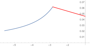
Figure 3: The crossing between $|g_{1}(t)|$ (red) and $|g_{2}(t)|$ (blue) at $t=t_{\ast}\simeq-2.83240$. Only the minimum between the two curves is shown.

After a further interval, where the singularity at $g_{1}$ is encountered first and the behavior is the same as in $-1\leq t<0$, at a value $t_{\ast}$ we have $|g_{1}(t_{\ast})|=|g_{2}(t_{\ast})|$, then the solution $g_{2}$ wins. The numerical value of $t_{\ast}$ is

$$t_{\ast} =-2.83240\dots$$ (100)

which corresponds to $R=-0.18470\dots$ via the relation $t^{-1}=\Phi^{\prime}(R)$. The value of $R$ satisfies the relatively simple equation

$$\Phi(R)-\big{(}R+\tfrac{1}{27}\big{)}\Phi^{\prime}(R)=-\Phi(\tfrac{1}{27})=\tfrac{1}{27}-\tfrac{\sqrt{3}}{12\pi}\,,$$ (101)

but we are not aware of any more explicit expression (e.g., as a root of a polynomial in $\mathbb{Q}[\sqrt{3}/\pi]$).

For $t\leq t_{\ast}$ (note, $t_{\ast}$ included) $R$ has a square-root singularity as in the case $t>0$. However, in this regime the resulting values of $R$ and $g$ are both negative. While analytic continuation for negative $g$ of a large-$N$ result in a matrix model is a well-understood and fundamental mechanism, see the example of the ‘basic’ quartic potential $V(M)=\tfrac{1}{2}M^{2}+\tfrac{1}{4}M^{4}$ [13], a negative value of $R$ is hard to interpret in light of its role in the Joukowski map.

In any case, the implication of this finding on the enumerative results seem clear, and state that, for $t\leq t_{\ast}$, the model exits the massless phase and is characterized by pure-gravity exponents. A very similar picture, and with a better analytical control, is presented in the case of cubic graphs, discussed in Section 4.7 below.

In the remainder of this section we will investigate the spectral density, and, because of the issue mentioned above, we restrict to $t>t_{\ast}$. The derivative of the potential is

$$W^{\prime}(z)=(1+t)z-\frac{2}{\sqrt{3}}\,t\sin\left(\tfrac{1}{3}\arcsin\left(\tfrac{3\sqrt{3}}{2}z\right)\right)\,,$$ (102)

and upon rescaling variables as

$$\lambda=ax=2\sqrt{R}x\,,$$ (103)

and denoting $\hat{\rho}(x)=\rho(ax)$, one gets from formula (54):

$$\hat{\rho}(x)=\frac{\sqrt{1-x^{2}}}{2\pi^{2}}\frac{1}{g}\fint_{-1}^{1}\,\mathrm{d}y\frac{W^{\prime}(2\sqrt{R}y)}{\sqrt{1-y^{2}}}\frac{1}{y-x}\,,\quad\text{supp}(\hat{\rho})=[-1,1]\,.$$ (104)

Using the integral

$$\fint_{-1}^{1}\frac{\,\mathrm{d}y}{y-x}\frac{\alpha+\beta y}{\sqrt{1-y^{2}}}=\beta\pi\,,\quad\text{for any }\alpha,\beta\,.$$ (105)

we get:

$$\hat{\rho}(x)=\frac{\sqrt{1-x^{2}}}{2\pi^{2}}\frac{1}{g}\left(2\pi(1+t)\sqrt{R}-\frac{2}{\sqrt{3}}\,t\fint_{-1}^{1}\,\mathrm{d}y\frac{\sin\big{(}\tfrac{1}{3}\arcsin\big{(}\sqrt{27R}y\big{)}\big{)}}{\sqrt{1-y^{2}}}\frac{1}{y-x}\right)\,.$$ (106)

In particular the critical density for $t_{\ast}<t<0$, using (95), reads as:

$$\hat{\rho}_{c}(x)=\frac{\sqrt{1-x^{2}}}{\sqrt{3}\pi^{2}}\frac{1}{g_{c}(t)}\left(\frac{\pi}{3}(1+t)-t\fint_{-1}^{1}\,\mathrm{d}y\frac{\sin\left(\tfrac{1}{3}\arcsin\left(y\right)\right)}{\sqrt{1-y^{2}}}\frac{1}{y-x}\right)\,.$$ (107)

We were not able to compute analytically the remaining integral. However, due to the simple form of (107), is is easily verified that $\hat{\rho}_{c}(x)$ is positive in its interval of definition for all values $t_{\ast}<t<0$.

We present in figure 4 the critical density for two different values of $t$. We note clearly the different slope at the spectral edge for $t_{\ast}<t<0$ and $t>0$ which entails the different critical exponents.

$$\begin{array}[]{ccc}\includegraphics[width=173.44534pt]{rhoc_quartic_t-05.pdf}&&\includegraphics[width=173.44534pt]{rhoc_quartic_Rc-01_tpos.pdf}\\ {t=-0.5\ (R=\frac{1}{27})}&&{t\simeq 3.23\ (R=\frac{1}{27}-0.01)}\end{array}$$

Figure 4: Critical spectral density for quartic graphs, rescaled to the interval $[-1,1]$ (of which, in light of symmetry, we show only the right half).

4.6 Generalization to arbitrary even degree

The quartic case shows the main features of all the cases of even degree. For arbitrary $h=2p$, with $p\in\mathbb{N}$, $S=0$ because of symmetry, and (60) reduce to

$$v =R-t\,\Phi(R)\,, \Phi(R) =\sum_{n\geq 1}\frac{((2p+1)n)!}{(pn+1)!(pn)!}\frac{R^{pn+1}}{n!}\,.$$ (108)

Denoted the radius of convergence of $\Phi$ as

$$\tau_{h} =\frac{r_{h}^{2}}{4}=\frac{1}{4}\frac{h^{2}}{(h+1)^{2(h+1)/h}}\,,$$ (109)

(the first few values are $\tau_{h}^{h}=\frac{1}{64},\frac{1}{729},\frac{729}{4194304},\frac{256}{9765625},\ldots$), the series $\Phi(R)$ is the following hypergeometric series

$$\Phi(R)+R=R\;{}_{2p}F_{2p-1}\left(\tfrac{1}{2p+1},\tfrac{2}{2p+1},\dots,\tfrac{2p}{2p+1};\tfrac{1}{p},\tfrac{2}{p},\tfrac{2}{p},\tfrac{3}{p},\tfrac{3}{p},\dots,\tfrac{p}{p},\tfrac{p+1}{p};(R/\tau_{2p})^{p}\right)\,.$$ (110)

Apparently, this is an overwhelmingly complicated expression. Nonetheless, as we annotate later on, certain known properties of hypergeometric series are instrumental to establish the main features of the model.

We proceed as in the quartic case by computing the functions $v_{1}(t)$ and $v_{2}(t)$, for the singular triples $(t,R,v)$ satisfying one of the two singularity mechanisms, i.e. corresponding to the singularity of $\Phi$ at $R=\tau_{2p}$, and to $t^{-1}=\Phi^{\prime}(R)$, respectively.

$$v_{1}(t) =g_{1}^{1/p}(t)=(1+t)\tau_{2p}-\tau_{2p}C_{p}\,t\,,$$ (111)

$$v_{2}(t) =g_{2}^{1/p}(t)=R-\frac{\Phi(R)}{\Phi^{\prime}(R)}\Big{|}_{t^{-1}=\Phi^{\prime}(R)}\,,$$ (112)

where $C_{p}$ is defined as

$$C_{p}=\frac{\Phi(\tau_{2p})}{\tau_{2p}}+1\,.$$ (113)

Even though a closed form for $C_{p}$ is not easily available, it is remarkable that (111) is an affine function for all $p$’s.

The results that follow have been established numerically for the cases $p=1,2,3,4$, and conjectured to hold generally. One can extend the numerical analysis to bigger $p$ with no difficulties, and it should also be possible to prove these results (although we do not do this here). First of all, from the definition (108) it is easily evinced that $\Phi^{\prime}(R)$ is in fact a function of $R^{p}$, and in particular it has a useful symmetry under $\mathbb{Z}_{p}$ rotations of its argument

$$\Phi^{\prime}(z)=\Phi^{\prime}(\omega^{n}z)\,,\quad\omega=e^{2\pi i/p}\,,\quad n=0,1,\dots,p\,.$$ (114)

Given this symmetry, the analysis can be restricted to the cone

$$\left\{R=\rho e^{i\theta}\,\big{|}\,\rho\geq 0\,,\theta\in[0,\tfrac{\pi}{p}]\right\}\,.$$ (115)

We determined numerically the values of $R$ which give $\Im(\Phi^{\prime}(R))=0$, so that the equation $t^{-1}=\Phi^{\prime}(R)$ has a solution for real $t$. These lie on the boundary of the cone, in particular one has:

$$\Phi^{\prime}:(0,\tau_{2p})\cup\left\{\rho e^{i\pi/p}\,,\rho\in(0,\infty)\right\}\mapsto(0,+\infty)\cup(-1,0)\,,$$ (116)

and the region $(-\infty,-1)$ has no preimage under $\Phi^{\prime}$. (The point $t=-1$ corresponds to $R=\infty\times e^{i\pi/p}$.) Then, just as already observed in the $p=1$ case, the equation $\Phi^{\prime}(R)=t^{-1}$ has no solution for $t\in[-1,0]$.

For what concerns the regime $t>0$, it is then governed by exactly the same formulas (91–94), with $\Phi$ replaced by the appropriate series (108) and $g$ replaced by $v=g^{1/p}$, so the generating function for $t>0$ has the behaviour of pure gravity for any even degree. This holds for the same reasonings as in the quartic case, and doesn’t require any subtle control on the relevant expressions.

For $-1\leq t<0$, the singularity occurs at the critical radius of $\Phi$, since $t^{-1}=\Phi^{\prime}(R)$ has no solution. So $R_{c}=\tau_{2p}$ and the critical curve is:

$$v_{c}(t)=g_{c}^{1/p}(t)=(1+t)\tau_{2p}-\tau_{2p}C_{p}\,t\,.$$ (117)

The expression for $\tau_{2p}$ generalises (89), and the one above for $v_{c}(t)=(g_{c}(t))^{1/p}$ generalises (95). In the case $p=1$, we have $v_{c}(t)\geq 0$ for all $t<0$ as a result of the inequality $C_{1}-1=\frac{9\sqrt{3}}{4\pi}\geq 0$. The analogous statement here reads $C_{p}-1=\frac{\Phi(\tau_{2p})}{\tau_{2p}}\geq 0$, which holds at sight from the positivity of the series coefficients. More remarkably, since

$$\psi_{2p-1}=\tfrac{1}{p}+\tfrac{2}{p}+\tfrac{2}{p}+\tfrac{3}{p}+\tfrac{3}{p}+\dots+\tfrac{p}{p}+\tfrac{p+1}{p}-\left(\tfrac{1}{2p+1}+\tfrac{2}{2p+1}+\dots+\tfrac{2p}{2p+1}\right)=1\,,$$ (118)

general results on hypergeometric series imply that for any $p$ the leading singular term in the expansion of $\Phi$ around $\tau_{p}$ is $\log(\delta)\delta$, where we defined $\delta$ as before, $R=\tau_{2p}(1-\delta)$. For example, in the case $p=2$ (i.e., graphs of degree six), equation (96) is modified into

$$\epsilon \sim D\,t\,\log(\delta)\delta\,, D =\frac{\sqrt{5}}{4\pi}\frac{R_{c}}{\sqrt{g_{c}}}\,.$$ (119)

We now move to the region $t<-1$. According to formula (116), the preimage of this region under $\Phi^{\prime}$ is the ray $\rho e^{i\pi/p}\,,\rho\in(0,\infty)$. The phenomenology is exactly the same as in the quartic case. By comparing $|v_{1}|$ and $|v_{2}|$ one establishes the existence a critical value $t_{\ast}$ such that the singularity given by $t^{-1}=\Phi^{\prime}(R)$ takes over that due the lack of analyticity at $\tau_{2p}$, and implies the pure gravity scaling exponent. The values of $t_{\ast}$ determined are reported in the following table together with $R_{\ast}$, $t_{\ast}^{-1}=\phi^{\prime}(R_{\ast})$:

$h=2p$	$t_{\ast}$	$R_{\ast}e^{\pi i(n+1/p)}$	$|g_{\ast}|$
2	$-2.83240\dots$	$0.184609\dots$	$0.0622653\dots$
4	$-3.44339\dots$	$0.189499\dots$	$0.00920182\dots$
6	$-3.95672\dots$	$0.194037\dots$	$0.00163489\dots$
8	$-4.40930\dots$	$0.197990\dots$	$0.000317077\dots$

The multiplicity of choices for the argument of $R_{\ast}$ ($0\leq n<p$ in the notation above) reflects the aforementioned $\mathbb{Z}_{p}$ symmetry of $\Phi^{\prime}(R)$. We note that the absolute values of both $t_{\ast}$ and $R_{\ast}$ slightly increase with $p$. Even worse than in the case $p=1$, for $t\leq t_{\ast}$ the interpretation of $R$ in terms of the support of the (supposedly one-cut) spectral density seems to breaks down.

Finally, the above findings imply that all values of $p$ show the same universal critical behavior, while (as expected) the critical value $t_{\ast}$ is not universal.

4.7 The case of cubic graphs

In the case of cubic graphs, the potential has a more explicit expression, and is thus of a more tractable form that in case of higher degree. In particular, we have for the derivative

$$W^{\prime}(z)=(1+t)z+\frac{t}{2}(-1+\sqrt{1-4z})\,.$$ (120)

On the other side, equations (60) are now more complicated than in the cases analysed in the previous sections, since $S\neq 0$. For these reasons, we analyse this case starting from the integral constraints (55). This approach is different from the analysis of the cubic case in [35], while it essentially coincides with the one of [36].

Instead of dealing with $R$ and $S$, we work here directly with $a_{1}$ and $a_{2}$ (recall that the two pairs of parameters are related by (56)). In order to proceed, we shall need the following integrals (valid for $a_{2}<1/4$, as is the case here)

$$\int_{a_{1}}^{a_{2}}\,\mathrm{d}\mu\frac{A+B\mu}{\sqrt{(\mu-a_{1})(a_{2}-\mu)}}=\pi\left(A+B\frac{a_{1}+a_{2}}{2}\right)\,,$$ (121)

$$\int_{a_{1}}^{a_{2}}\,\mathrm{d}\mu\sqrt{\frac{1-4\mu}{(\mu-a_{1})(a_{2}-\mu)}}=2\sqrt{1-4a_{1}}E\left(4\frac{a_{2}-a_{1}}{1-4a_{1}}\right)\,,$$ (122)

$$\int_{a_{1}}^{a_{2}}\,\mathrm{d}\mu\sqrt{\frac{\mu-a_{1}}{a_{2}-\mu}}(A+B\mu)=\pi\frac{a_{2}-a_{1}}{2}\left(A+B\frac{a_{1}+3a_{2}}{4}\right)\,,$$ (123)

$$\begin{split}&\int_{a_{1}}^{a_{2}}\,\mathrm{d}\mu\sqrt{\frac{(\mu-a_{1})(1-4\mu)}{a_{2}-\mu}}=\\ &\quad\tfrac{4}{3}\sqrt{\tfrac{1}{4}-a_{1}}\left(\left(\tfrac{1}{4}-a_{2}\right)K\left(4\frac{a_{2}-a_{1}}{1-4a_{1}}\right)+\left(2a_{2}-a_{1}-\tfrac{1}{4}\right)E\left(4\frac{a_{2}-a_{1}}{1-4a_{1}}\right)\right)\,,\end{split}$$ (124)

where $K(m),E(m)$ are the complete elliptic integrals of the first and second kind with parameter (square of elliptic modulus) $m$. The less trivial equations (122) and (124) can be found in [60, eqs. (3.141.2) and (3.141.26)]. Equations (55) then read as

$$(1+t)\pi\frac{a_{1}+a_{2}}{2}-\frac{t}{2}\pi+t\sqrt{1-4a_{1}}E\left(4\frac{a_{2}-a_{1}}{1-4a_{1}}\right) =0\,,$$ (125)

$$\begin{split}-t\pi\frac{a_{2}-a_{1}}{4}+(1+t)\pi\frac{(a_{2}-a_{1})(a_{1}+3a_{2})}{8}\qquad\qquad&\\ +\tfrac{t}{12}\sqrt{1-4a_{1}}\left(\left(1-4a_{2}\right)K\left(4\tfrac{a_{2}-a_{1}}{1-4a_{1}}\right)+\left(8a_{2}-4a_{1}-1\right)E\left(4\tfrac{a_{2}-a_{1}}{1-4a_{1}}\right)\right)&=2\pi g^{2}\,.\end{split}$$ (126)

The spectral density can be derived from equation (54). At this aim it is convenient to perform an affine change of coordinates as to set the support of the density on $[-1,1]$: let us change coordinates as

$$\lambda :=f(x)=Ax+B\,, A =\frac{a_{2}-a_{1}}{2}\,, B =\frac{a_{1}+a_{2}}{2}\,,$$ (127)

and let us call $\hat{\rho}(x)\equiv\rho(f(x))$ the resulting distribution. Then we have

$$\hat{\rho}(x) =\frac{\sqrt{1-x^{2}}}{2\pi^{2}g^{2}}\fint_{-1}^{1}\frac{\,\mathrm{d}y}{y-x}\frac{W^{\prime}(f(y))}{\sqrt{1-y^{2}}}$$ (128)

$$=\frac{\sqrt{1-x^{2}}}{2\pi^{2}g^{2}}\left((1+t)A\pi+t\sqrt{A}\fint_{-1}^{1}\frac{\,\mathrm{d}y}{y-x}\sqrt{\frac{\frac{1-4B}{4A}-y}{1-y^{2}}}\right)\,.$$ (129)

where we used the integral (105). The parameters $A$ and $B$ as a function of $t$ are to be determined in what follows.

The analysis of [35] shows that, in the regime $t>0$, cubic and quartic graphs behave similarly, and in both cases this corresponds to a massive phase on the flat lattice. This could be rederived here, but the procedure and conclusions are similar to the ones already depicted for the case of even degree, and are comparatively less interesting than the behaviour at negative values of the fugacity.

Thus, we will focus our attention directly on the regime $t<0$, where, yet again, at least in an interval containing $t\in[-1,0]$, and possibly extending below $t=-1$, criticality is expected to appear as the support of the spectral density touches the boundary of the analyticity region of $W$. The function $W$ can be analytically continued to the complex plane minus the cut on the real axis $z\geq 1/4$, so in this interval the critical value is $a_{2,c}=1/4$, while $a_{2,c}<1/4$ if the criticality mechanism is different. For convenience, in the following we will trade $a_{1}$ for an equivalent variable defined as

$$s=\sqrt{1-4a_{1}}\,.$$ (130)

As $a_{2}\leq 1/4$, and $a_{1}<a_{2}$, we have that $s>0$.

At a critical point with $a_{2}=1/4$, the above equations reduce to algebraic ones:

$$s^{2}(t+1)+2(t-1) =\frac{8}{\pi}st$$ (131)

$$s^{4}(t+1)+4s^{2}(t-1)-\frac{32}{3\pi}s^{3}t =-256g^{2}\,.$$ (132)

Solving the first for $s$, with the condition $s>0$, gives:

$$s_{c} =\frac{1}{\pi}\frac{4t+\sqrt{2}\sqrt{\pi^{2}-\left(\pi^{2}-8\right)t^{2}}}{1+t}\,,$$ (133)

valid within the interval $t_{\ast}\leq t<0$, with $t_{\ast}$ defined as

$$t_{\ast}\equiv-\frac{\pi}{\sqrt{\pi^{2}-8}}=-2.2976\dots$$ (134)

Therefore, plugging $s_{c}$ in (132), we have that, provided that the leading criticality mechanism comes from the singularity of $W$ at $1/4$, the critical values of the parameters as functions of $t$ are

$$a_{2,c} =\frac{1}{4}\,,$$ (135)

$$a_{1,c} =\frac{1}{4}-\frac{1}{4\pi^{2}}\frac{\big{(}4t+\sqrt{2\pi^{2}-2\left(\pi^{2}-8\right)t^{2}}\big{)}^{2}}{(1+t)^{2}}\,,$$ (136)

$$g_{c}^{2} =\frac{(4t+\sqrt{2}\sqrt{8t^{2}+\pi^{2}(1-t^{2})})^{3}(-4t+3\sqrt{2}\sqrt{8t^{2}+\pi^{2}(1-t^{2})})}{768\pi^{4}(t+1)^{3}}$$ (137)

$$=\frac{512t^{4}+96\pi^{2}\left(1-t^{2}\right)t^{2}+16\sqrt{2}\left(8t^{2}+\pi^{2}\left(1-t^{2}\right)\right)^{3/2}t+3\pi^{4}\left(1-t^{2}\right)^{2}}{192\pi^{4}(t+1)^{3}}\,.$$ (138)

We have also determined that this criticality pattern may occur at most on the interval $t_{\ast}\leq t<0$ (and we know in advance, from [35], that it occurs at least on the interval $-1\leq t<0$). Later on, we determine that the interval in which this criticality pattern is dominant is $t_{\ast}<t<0$.

Note that the formula (138) above coincides with the expression for the critical radius of the series first obtained in [35, eq. (77)], of which it thus provides an alternate derivation. At $t=t_{\ast}$, the expressions for $g^{2}_{c}$ and $a_{1,c}$ simplify considerably:

$$g^{2}_{c}(t_{\ast}) =\frac{1}{3(\pi^{2}-8)^{2}(\frac{\pi}{\sqrt{\pi^{2}-8}}-1)^{3}}$$ (139)

$$a_{1,c}(t_{\ast}) =\frac{1}{4}-\frac{4}{(\pi-\sqrt{\pi^{2}-8})^{2}}\,.$$ (140)

To compute the critical exponents in the range $t_{\ast}\leq t<0$, we investigate the behaviour close to the critical point. We set $g^{2}=g_{c}^{2}(1-\epsilon)$, $a_{2}=a_{2,c}(1-\delta)$, $s=s_{c}(1-\eta)$ and consider the limits $\epsilon$, $\delta$ and $\eta\to 0^{+}$. The goal is to compute the singularity of the partition function from (80), which is

$$Z^{\prime\prime}\sim 2\frac{N^{2}}{g_{c}^{4}}\log(\tfrac{1}{4}s_{c}^{2}+\tfrac{1}{4}\delta-\tfrac{1}{2}s_{c}^{2}\,\eta)\,,$$ (141)

and requires computing the dependence of $\eta$ and $\delta$ on $\epsilon$. If we write equation (125) in terms of $\eta$ and $\delta$, and expand around $\delta=0$, we have

$$\left(2s_{c}(-4t+\pi s_{c}(1+t))\eta-\pi s_{c}^{2}(1+t)\eta^{2}\right)s_{c}(1-\eta)=2t\delta\log(\delta)+o(\delta\log(\delta))\,.$$ (142)

Note that $o(\delta\log(\delta))$ contains also terms of the type $\eta\delta\log(\delta)$, and that the coefficient of $\eta$ on the l.h.s. is positive for $t_{\ast}<t<0$, while it vanishes at $t_{\ast}$:

$$(-4t+\pi s_{c}(1+t))|_{t=t_{\ast}}=0\,.$$ (143)

We start by analysing the case $t>t_{\ast}$. In this case we can neglect the order $\eta^{2}$ on the l.h.s., and the subleading terms on the r.h.s., and the equation above gives:

$$\eta(1+\mathcal{O}(\eta))=\frac{t}{s_{c}^{2}(-4t+\pi s_{c}(1+t))}\delta\log(\delta)\,.$$ (144)

We can now look at equation (126), which, after expansion, reads

$$\begin{split}128g^{2}_{c}\pi\epsilon+o(\epsilon)=\eta^{2}s_{c}^{2}\left(\pi\left(3s_{c}^{2}(t+1)+2(t-1)\right)-16s_{c}t\right)+o(\eta^{3})\\ +4s_{c}\,t\,\delta\log(\delta)+o(\delta\log(\delta))\,,\end{split}$$ (145)

Note that the coefficient of order $\eta$ is identically zero for any $t$. Using (144), the terms of order $\eta^{2}$ and higher can again be neglected, and $\delta$ can be expressed in terms of $\epsilon$ as in (98). In conclusion, for $t_{\ast}<t<0$ we have

$$\eta \sim-2\alpha\,\epsilon\,, \alpha =-\frac{64g_{c}^{2}\pi}{s_{c}^{3}(-4t+\pi s_{c}(1+t))}\,,$$ (146)

$$\delta \sim s_{c}\beta\,\frac{\epsilon}{\log(\epsilon)}\,, \beta =\frac{32g_{c}^{2}}{s_{c}^{2}t}\,.$$ (147)

The $\epsilon$–dependent part of the partition function is, with $\alpha$ and $\beta$ as above,

$$Z^{\prime\prime}\sim\frac{2N^{2}}{g_{c}^{4}}\left(\alpha\epsilon+\beta\frac{\epsilon}{\log(\epsilon)}\right)\,,\quad\text{for }t_{\ast}<t<0\,,$$ (148)

This coincides with the singular behaviour found in [35, Eq. 78], where $Z^{\prime\prime}$ is there called $F^{\prime}$. The term proportional to $\alpha$ is non–singular and does not affect the large-$n$ behavior of the coefficients $Z_{n}$, which thus have the same form as in the quartic case: $Z_{n}\sim g_{c}^{-n}n^{-4}\log^{-2}(n)$.

We now turn our attention to the case $t=t_{\ast}$ (which was not discussed in [35]). Then, as already remarked, the coefficient of $\eta$ in (142) is zero. On the l.h.s. of (142) the leading term is of order $\eta^{2}$, while the r.h.s. is unchanged, since terms of the form $\eta\delta\log(\delta)$ are still suppressed compared to $\delta\log(\delta)$. Therefore one obtains:

$$\eta=\frac{\pi-\sqrt{\pi^{2}-8}}{4\sqrt{2}}\sqrt{-\delta\log(\delta)}\,.$$ (149)

Now we have to take into account the $\eta^{2}$ term in Eq. (145), which is of the same order as the summands involving $\delta\log(\delta)$. However, the coefficient multiplying $\eta^{2}$ is exactly zero at $t=t_{\ast}$,

$$\left(\pi\left(3s_{c}^{2}(t+1)+2(t-1)\right)-16s_{c}t\right)|_{t=t_{\ast}}=0\,,$$ (150)

the first non-vanishing term in $\eta$ is of order $\eta^{3}\sim(\delta\log(\delta))^{3/2}$, and therefore negligible. Thus, for $t=t_{\ast}$ we find

$$\eta \sim\frac{1}{2\sqrt{3}}\epsilon^{1/2}\,, \delta \sim-\frac{8}{3\pi(\pi-\sqrt{\pi^{2}-8})^{2}}\frac{\epsilon}{\log(\epsilon)}\,,$$ (151)

and the partition function is:

$$Z_{\text{sing}}^{\prime\prime}\sim-\frac{2N^{2}}{g_{c}^{4}}\left(\frac{1}{\sqrt{3}}\epsilon^{1/2}+\frac{1}{6\pi}\frac{\epsilon}{\log(\epsilon)}\right)\,.$$ (152)

The leading singular behavior is thus $\epsilon^{1/2}$, which corresponds to pure gravity, even though it comes along with peculiar subleading corrections, with the exponents (and logarithms) of the Berker–Kadanoff phase.

Thus, we have determined that the massless phase, which is the quantum gravity counterpart of the Berker–Kadanoff phase and which is characterized by $\gamma=-1$, $\gamma^{\prime}=-2$ leading singularity, occurs for cubic graphs in the region $t_{\ast}<t<0$, while at the point $t=t_{\ast}$ the spanning forest model has a critical point characterized by the pure gravity critical exponent.

We shall now discuss the region $t<t_{\ast}$. Before doing this, let us come back to the expression (129) for the spectral density. Let us introduce a shortcut $d=\frac{1-4B}{4A}\geq 1$ for this recurring combination. The integration in principal value on the variable $y$ can be performed. When $d>1$, the remaining integral is [60, 3.131.3,3.137.3]:

$$\begin{split}\fint_{-1}^{1}&\frac{\,\mathrm{d}y}{y-x}\sqrt{\frac{d-y}{1-y^{2}}}=-\frac{2}{\sqrt{d+1}}K\left(\frac{2}{d+1}\right)\\ &-\frac{2}{\sqrt{d+1}}\frac{d-x}{x+1}\left(\Pi\left(\frac{2}{x+1}\Big{|}\frac{2}{d+1}\right)-\frac{\pi}{2}\sqrt{\frac{(x+1)(d+1)}{(x-1)(d-x)}}\right)\,,\end{split}$$ (153)

where $\Pi(n|k^{2})$ is the complete elliptic integral of third kind with elliptic characteristic $n$ and modulus $k$. When $a_{2}=a_{2,c}=1/4$, corresponding to $d=\frac{1-4B}{4A}=1$, the integral simplifies considerably, and just gives

$$\fint_{-1}^{1}\frac{\,\mathrm{d}y}{y-x}\frac{1}{\sqrt{1+y}}=\frac{2}{\sqrt{x+1}}\log\left(\frac{\sqrt{2}-\sqrt{x+1}}{\sqrt{1-x}}\right)\,.$$ (154)

Thus, for $t_{\ast}\leq t<0$ the critical density is:

$$\begin{split}\hat{\rho}_{c}(x)&=\frac{\sqrt{1-x^{2}}}{2\pi^{2}g^{2}_{c}}\left((1+t)A_{c}\pi+\frac{2\,t\sqrt{A_{c}}}{\sqrt{x+1}}\log\left(\frac{\sqrt{2}-\sqrt{x+1}}{\sqrt{1-x}}\right)\right)\,,\\ A_{c}&=\tfrac{1}{2}(\tfrac{1}{4}-a_{1,c})\,.\end{split}$$ (155)

where $a_{1,c}$ and $g_{c}$ are as in equations (135) and (137). It is easily verified that the density is positive, and that at the edges it behaves as

$$\hat{\rho}_{c}(x) =\frac{t\sqrt{A_{c}}}{2\pi^{2}g^{2}_{c}}\sqrt{1-x}\;\big{(}\log(1-x)+\mathcal{O}(1)\big{)}$$ (156)

$$=\frac{\sqrt{2}\pi(t+1)A_{c}-2t\sqrt{A_{c}}}{2\pi^{2}g_{c}^{2}}\sqrt{1+x}\;\big{(}1+\mathcal{O}(1+x)\big{)}$$ (157)

At the right edge there is the logarithmic singularity responsible for the peculiar critical behaviour of the model, while at the left edge the behavior is instead the ‘ordinary’ non-critical one, i.e. a square-root singularity. We note that $g_{c}$ and $A_{c}$ are both strictly positive in the range $t\in[t_{\ast},0]$, while the coefficient of $\sqrt{1+x}$ in the expansion around $x=-1$ is positive only for $t\in(t_{\ast},0]$ and is zero exactly at $t=t_{\ast}$. Therefore, at $t=t_{\ast}$ we see the occurrence of the phase transition discussed above, and the behavior at the left spectral edge becomes $\sim(x+1)^{3/2}$. This is similar in form to what happens in the simplest criticality mechanism, leading to the pure-gravity exponent in one-matrix models of random matrix theory [13], and it is consistent with the pertinent singularity of the partition function discussed above. In particular, it proves in retrospective that in the range $t\in[t_{\ast},0]$ we had identified the leading criticality mechanism.

We will now identify the critical behaviour of pure gravity in all the regime $t\leq t_{\ast}$. At this aim we show that, in this regime, there exist critical values $a_{1}(t)$, $a_{2}(t)$ such that the spectral density has a $(x+1)^{3/2}$ singular behaviour at $x=-1$. We start by expanding the density (153) around $x=-1$, using well-known properties of elliptic functions:

$$\hat{\rho}(x) =\frac{t\sqrt{A}\sqrt{1+x}}{\sqrt{2}\pi^{2}g^{2}}\,\big{(}1-\tfrac{1}{4}(x+1)+O((x+1)^{2})\big{)}\,\big{(}R_{0}+R_{1}(x+1)+O((x+1)^{2})\big{)}\,;$$ (158)

$$R_{0} =\frac{1+t}{t}\sqrt{A}\pi+\frac{(d-1)}{\sqrt{d+1}}K\left(\tfrac{2}{d+1}\right)-\sqrt{d+1}E\left(\tfrac{2}{d+1}\right)\,;$$ (159)

$$R_{1} =\frac{1}{3}\left(\frac{d-1}{\sqrt{d+1}}K\left(\tfrac{2}{d+1}\right)-\frac{d}{\sqrt{d+1}}E\left(\tfrac{2}{d+1}\right)\right)\,.$$ (160)

In order for the density to have a $(x+1)^{3/2}$ singularity, we need to impose that $R_{0}=0$ (and verify that $R_{1}\neq 0$ ). This fixes a relation among $t$, $A$ and $d$, that, together with (125), gives the critical values for $A$ and $d$ as functions of $t$. From

$$a_{1} =\frac{1}{4}-A(d+1)\,, a_{2} =\frac{1}{4}-A(d-1)\,,$$ (161)

we get the system:

$$\frac{t+1}{t}=\frac{2}{\pi(1-4Ad)}\left(\pi-4\sqrt{A(d+1)}E\left(\tfrac{2}{d+1}\right)\right)\,,$$ (162a)

$$\frac{t+1}{t}=\frac{1}{\sqrt{A}\pi}\left(\sqrt{d+1}E\left(\tfrac{2}{d+1}\right)-\frac{d-1}{\sqrt{d+1}}K\left(\tfrac{2}{d+1}\right)\right)\,.$$ (162b)

We satisfy the conditions $a_{1}<a_{2}\leq 1/4$ if and only if $A>0$ and $d\geq 1$. As a first check we discuss again $d=1$. In this case, we shall find that $t=t_{\ast}$ is a solution. The system above simplifies to

$$\frac{t+1}{t} =-\frac{8\sqrt{2A}-2\pi}{\pi(1-4A)}\,, \frac{1+t}{t} =\frac{\sqrt{2}}{\sqrt{A}\pi}\,.$$ (163)

There are two solutions:

$$A_{\pm}(d=1)=\frac{1}{16}\left(-4+\pi^{2}\pm\pi\sqrt{\pi^{2}-8}\right)=\{0.635326,0.0983747\}\,,\quad t=\pm t_{\ast}\,.$$ (164)

This confirms our previous result that at $t=t_{\ast}$ the left edge has a $(x+1)^{3/2}$ singularity. Conversely, the $(x+1)^{3/2}$ singularity at $t=-t_{\ast}$ is shadowed by the $(1-x)^{3/2}$ singularity, that occurs before.

For $d>1$ the picture remains similar, although the expressions are less explicit. The triple $(t,A,d)$ with appropriate singularity, at $t=t_{\ast}$ and $d=1$, is deformed continuously, and monotonically in the three parameters, as $d$ grows, the limit of $t$ for $d\to\infty$ being $t=-\infty$. The spurious branch at $t=-t_{\ast}$ and $d=1$, similarly, is also deformed monotonically (this time, with $t$ increasing, instead that decreasing), so it is always shadowed by the criticality at the other endpoint of the support.

A convenient way of expressing the general result is to derive, by mean of (162), parametric expressions $A(d)$ and $t(d)$, to be analysed in the regime $d\geq 1$. We obtain two branches for the function $A(d)$, which in turn give two branches for $t(d)$. For the reasons discussed above, we have to keep only the branch with negative values of $t$ (which, indeed, is a monotonic function with image $(-\infty,t_{\ast}]$). These expressions can be used, for example, to plot $a_{1}(t)$ and $a_{2}(t)$ in this range of parameters, as shown in Figure 5.

Figure 5: The support of the spectral density for $t\leq t_{\ast}$.

5 Complex zeroes of $R_{k}(t)$ and $Z_{k}(t)$

Both in the case of $h$ even and odd, the behaviour at and below $t_{\ast}$, where the Berker–Kadanoff phase has its lower endpoint and the system is again massive, is an interesting new element w.r.t. the treatment of [35], and deserves some deeper investigation.

In this short section we inspect more closely the numerical series $R(g,t)$ and $Z(g,t)$. Let us call $R_{k}(t)$ and $Z_{k}(t)$ the polynomials in $t$ associated to these series

$$R(g,t) =g+\sum_{k\geq 2}g^{k}t\;R_{k}(t) Z(g,t) =\sum_{k\geq 2}g^{k}\;Z_{k}(t)$$ (165)

We know for sure that the $Z_{k}(t)$’s are real-positive if $t\geq-1$. This is a consequence of the fact that these quantities can be written as a sum over trees, with non-negative weights (this is detailed in Section 6).

The quantities $Z_{k}(t)$ may or may not become negative for values $t<-1$. Our numerical observations are compatible with the following conjectures.

For $h=1$, at $t>t_{\ast}$ there exists a value $n_{0}(t)$ such that $Z_{k}(t)<0$ if $k<n_{0}$ and $Z_{k}(t)\geq 0$ if $k\geq n_{0}$, while at $t\leq t_{\ast}$ all $Z_{k}(t)$ are negative. In other words, all the polynomials $Z_{k}(t)$ have a unique real root $t_{0}(k)$, these roots form a monotonically decreasing sequence, with limit $t_{\ast}^{(h=1)}$.

For $h=2$, $Z_{2k}(t)>0$ for all values of $t$, while $Z_{2k+1}(t)$ have a pattern similar to the one of the $Z_{k}$’s for $h=1$, i.e., each polynomial has a unique real root $t_{0}(k)$, and these roots form a monotonically decreasing sequence, with limit $t_{\ast}^{(h=2)}$.

The fact that, for $h=2$ and $t<t_{\ast}$, the coefficients of the series alternate in sign is compatible with the finding of Section 4.5, where it is evinced that at $t\leq t_{c}$ the main singularity is present for a negative value of $g$. Similar patterns emerge for the polynomials $R_{k}(t)$.

More generically, it is interesting to investigate the roots in the complex plane of the polynomials $R_{k}(t)$ and $Z_{k}(t)$. Indeed, it turns out that these roots have a simple behaviour, and seem to accumulate on some ‘C-shaped’ curve in the complex plane. It is the symmetry of this curve that determines the sign behaviour depicted above: as the roots come in complex-conjugate pairs except for the ones on the real axis, if we assume that all the roots are aligned, roughly along this curve, then it follows that there is exactly one real root, or no real root at all, if the polynomial has odd or even degree, respectively.

We will present data for the polynomials $Z_{k}(t)$ in the case $h=1$ and $h=2$ (data for the $R_{k}$’s, and, at $h=1$, for $S_{k}$’s, are qualitatively similar). Before doing this, we solve exactly a ‘toy version’ of the system of equations relating $R$, $S$ and $Z$, which shows explicitly the features depicted above.

5.1 The toy model

Consider the equation

$$R=g+t\,\Phi(R)$$ (166)

with the choice

$$\Phi(R)=\frac{R(1-\sqrt{1-4R})}{2}=R^{2}\big{(}1+R\;{}_{2}F_{1}(1,\tfrac{3}{2};3;4R)\big{)}\,.$$ (167)

The second equality shows the analogy with the equations appearing in our model, see e.g. equation (88).

This equation is sufficiently simple that it can be solved for $R=R(g,t)$

$$R(g,t)=g+\sum_{i=1}^{\infty}\sum_{j=1}^{i}\frac{(i+j)!(2i-j-1)!}{i!(i+1)!(i-j)!(j-1)!}g^{i+1}t^{j}$$ (168)

The polynomials $R_{k}(t)=t^{-1}[g^{k+1}]R$ are thus, up to an overall factor,

$$R_{k}(t)\propto\sum_{j=0}^{k}t^{j}\binom{k}{j}\bigg{/}\binom{3k+2}{2k-j}$$ (169)

(curiously enough, up to a factor $1/((k+j+1)(k+j+2))$, these polynomials are proportional to the celebrated refined enumerations of Alternating Sign Matrices [61]).

Now, for $t$ to be a zero of such a polynomial, we shall have

$$\sum_{j}\exp\Big{(}j\ln t+\ln(2k-j)!+\ln(k+j+2)!-\ln j!-\ln(k-j)!\Big{)}=0\,.$$ (170)

In the limit of large $k$, calling $x=j/k$ and $\ell(x)=x\ln(x)$, we shall have

$$\int_{0}^{1}dx\exp(k\,S(x,t)) =0$$ (171)

with

$$S(x,t) =x\ln t+\ell(2-x)+\ell(1+x)-\ell(x)-\ell(1-x)$$ (172)

The integral is dominated by (one or more of) the saddle points, which in this case are at the positions

$$x_{\pm}(t)=\frac{-1\pm\sqrt{1-t+t^{2}}}{-1+t}$$ (173)

The two saddle points coincide when $t=t_{\pm}:=\exp(\pm i\pi/3)$. The integrand is not zero at none of the saddle points, so the only possibility for the integral to vanish is that the contributions at the two saddle points are equal in absolute value, and of opposite phase. The phase varies rapidly, and shall be discarded (its leading variation rate would determine the asymptotic density of the roots of the polynomials on the limit curve, but we do not perform this calculation here). The necessary condition on the absolute value, namely $Re(S(x_{+}(t),t)-S(x_{-}(t),t))=0$, is verified on four arcs:

• the arc of the circle of radius 1 and center 0, at the left of $t_{\pm}$;

• the arc of the circle of radius 1 and center 1, at the right of $t_{\pm}$;

• the straight segment connecting $t_{\pm}$;

• the two straight segments, connecting $t_{+}$ with $+i\infty$ and $t_{-}$ with $-i\infty$ (this is a single arc in the Riemann sphere).

It turns out that the roots of the polynomials are asymptotically supported on the first of the four arcs mentioned above.

See Figure 6 for an illustration of the properties discussed above.

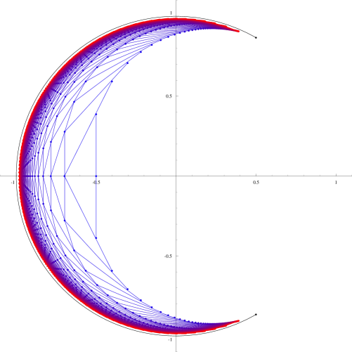
Figure 6: Roots of the polynomials $R_{k}(t)$ defined in (169), for $k\leq 80$, and their limit curve.

5.2 The true model

Here we show the numerical results for the ‘true’ quantities in our model, for the cases $h=1$ (Figure 7) and $h=2$ (Figure 8).

From the discussions in Section 4.5 and 4.7, we know the point of intersection of the limit curve with the horizontal axis (see equations (100) and (134)). It would be interesting to determine also the limit curves, and in particular their endpoints.

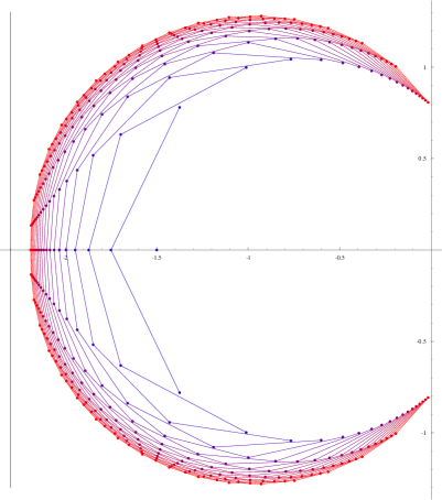
Figure 7: Roots of the polynomials $Z_{k}(t)$ in the model at $h=1$, for $k\leq 20$. The vertical segment marks the limit of the real roots, $t_{\ast}=-\frac{\pi}{\sqrt{\pi^{2}-8}}=-2.2976\ldots$

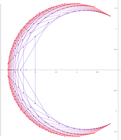
Figure 8: Roots of the polynomials $Z_{k}(t)$ in the model at $h=2$, for $k\leq 25$. The vertical segment marks the limit of the real roots, $t_{\ast}=-2.8324\ldots$

6 The Berker–Kadanoff phase at t = -​-1

6.1 The role of Bernardi embedding-activities

The partition function (1) of spanning forests over a given graph $G$ corresponds to a (monovariate) specialization of the (bivariate) Tutte polynomial $T_{G}(x,y)$ associated to a graph $G$ (see e.g. [2]), namely

$$Z^{\mbox{\scriptsize{forest}}}_{G}(t,1)=t\;T_{G}(t+1,1)\,.$$ (174)

The Tutte polynomial admits both a formulation in terms of spanning subgraphs, and one as a sum over spanning trees weighted according to their activities [1]. The latter is particularly useful when studying $T_{G}(x,y)$ for $x,y\geq 0$, but not both $\geq 1$, so that the weights associated to spanning subgraphs are not real-positive, but those associated to trees are.

Activities are of two kinds. An edge in the tree may be internally-active, while one not in the tree may be externally-active. The $t=-1$ point of spanning forests is specially simple. Externally-active edges have weight 1, so we do not need to ‘count’ them. Internally-active edges have weight 0, so they are just forbidden. This simplifies the combinatorics: once an internally-active edge has been identified in the tree, we can discard the associated term, with no need to complete the exploration. The partition function at fixed graph is an integer, and thus also the generating function associated to random planar graphs has integer-valued coefficients, provided we take an ensemble of suitably ‘rooted’ graphs, so that the automorphism group is trivialised.

The concrete determination of internally-active edges is not a natural task. Tutte’s definition of activities is associated to an arbitrary but fixed labeling of the edges, which is not a canonical notion. Alternatively, it could be defined as an average over all possible labelings, but this would introduce a new set of variables, which makes the treatment complicated.

Luckily enough, by a breakthrough result of Bernardi [62] we now know that, for graphs embedded on a surface, one can define embedding-activities, i.e. activities determined in terms of a canonical labeling of the edges associated to the tree. Remarkably, and for non-trivial reasons, the Tutte polynomial based on ‘static’ activities and the Bernardi polynomial using embedding activities do coincide.

This result makes viable a probabilistic analysis of large random planar graphs equipped with a ferromagnetically-critical Potts model at $0\leq q\leq 4$, somewhat along the lines by which the same limit is constructed for pure gravity, an approach that has flourished in recent years [63, 64, 65, 66, 67]. However, unfortunately, this probabilistic approach seems to be confined to the ferromagnetic critical line, thus it is orthogonal to the treatment of spanning forests, except that at the trivial spanning-tree criticality.

6.2 Reformulation in terms of spanning trees with internal activities

Consider a graph $G$, embedded on a surface, and with a distinguished half-edge (the root). Given a spanning tree $T$ over it, we say that an edge is internal if it belongs to the tree, and external otherwise. Define the fundamental cocycle of an internal edge $e$ as the set of external edges $f$ such that $T\backslash\{e\}\cup\{f\}$ is a spanning tree. I.e., removing $e$ from the tree leaves with two components, and the cocycle is the set of edges with endpoints on distinct components. Analogously, define the fundamental cycle of an external edge $e$ as the set of internal edges $f$ such that $T\backslash\{f\}\cup\{e\}$ is a spanning tree. I.e., adding $e$ to the tree leaves with a unicyclic subgraph, and the cycle is just the cycle of the subgraph.

Now we consider a walk on the surface, encircling the tree, and starting from the root. Thus, we go along internal edges, while crossing external ones. Each internal edge happens to be adjacent to this walk exactly twice, one per side, The same happens for external edges, this time once per endpoint. Label internal and external edges according to the order of the first (of the two) visit by the walk.

This allows us to define the notion of activity: an external (resp. internal) edge is active if it is minimal in its fundamental cycle (resp. cocycle). Call ${\cal I}(T)$ and ${\cal E}(T)$ the number of internally- and externally-active edges of $T$, according to embedding-activities (this notation is somewhat elliptic, as this value depends on $G$ and on the root position as well). See Figure 9 for an example.

Figure 9: A rooted cubic random planar graph, equipped with a spanning tree. The exploration path around the tree is shown in blue, and determines the labeling of the edges (both internal and external). Active edges are denoted by labels in boldface (this example has $4$ internally- and $3$ externally-active edges).

Thus, as a corollary of Bernardi result [62], the spanning-forest partition function can be rewritten as

$$Z^{\mbox{\scriptsize{forest}}}_{G}(t,1)=t\sum_{T\preceq G}(1+t)^{{\cal I}(T)}\,.$$ (175)

As we said, embedding activities are more canonical than the original ones defined by Tutte. However, there is a tiny amount of non-canonical degrees of freedom left. First, we decided to explore the tree through a counter-clockwise contour. A clockwise contour would have produced the same polynomial, although the terms associated to the single trees would have been different. Second, we need to start the contour at some point, so that the tree is in fact rooted on a half-edge.

As we know, this is not unusual for random planar graphs, also in other models (and even just in pure gravity). The generating functions of unrooted and of rooted configurations are normally easily related one to another, while rooted ones have the advantage of avoiding graph automorphisms.

So, similarly to what is done in equation (4), to facilitate the combinatorics it is convenient to re-weight the sum. In this case we include a factor $|\mathop{\mathrm{Aut}}\nolimits(G)|/(3|V(T)|)$, so that the partition function for spanning forests on random planar graphs becomes:

$$Z(t,g) =\sum_{G\mathrm{~{}rooted}}\frac{g^{|V(T)|}}{3|V(T)|}\sum_{T\preceq G}(t+1)^{{\cal I}(T)}$$

$$=\sum_{T^{\prime}\mathrm{~{}rooted}}\frac{g^{|V_{\rm int}(T^{\prime})|}}{3|V_{\rm int}(T^{\prime})|}\sum_{L\in\mathcal{L}(T^{\prime})}(t+1)^{{\cal I}(T^{\prime})}\,.$$ (176)

In the second line the sum is over cubic planar trees $T^{\prime}$, and the restriction of $T^{\prime}$ to its non-leaf edges is the tree $T$. We also denote by $V_{\rm int}(T^{\prime})$ the set of non-leaf nodes of $T^{\prime}$, which thus coincides with all the nodes of $T$. There are $n_{T^{\prime}}=|V_{\rm int}(T^{\prime})|+2$ leaves. The set $\mathcal{L}(T^{\prime})$ is the ensemble of link patterns composed of $n_{T^{\prime}}/2$ arcs. Such a pattern, used for pairing the leaves of $T^{\prime}$, composes a graph $G$. The activities are then computed in this graph $G$ (so that ${\cal I}(T^{\prime})$ is a shorthand for the true dependence ${\cal I}(T^{\prime},L)$).

In the next section we will study this function at $t=-1$, which corresponds to counting configurations with no internally-active edge:

$$Z(-1,g)=\sum_{T}\frac{g^{|V(T)|}}{3|V(T)|}\sum_{L\in\mathcal{L}(T)}\delta_{{\cal I(T)},0}\,.$$ (177)

6.3 Recursion relations: resolving a branch

Let us consider the ensemble of planar rooted trees, and let us represent them as embedded in the lower half plane, and with leaves attached to the boundary, as in the lower part of Figure 9. We denote by ${\cal S}_{k,\ell}$ the subset of such trees, in which the vertices have all degree three, except for the root vertex, which has degree $k+\ell$. We further require that among these $k+\ell$ edges, the $\ell$ right-most vertices are leaves.

The position of infinity in the half-plane breaks the rotational symmetry among the edges adjacent to the root vertex, and we can canonically identify the root half-edge with the right-most edge adjacent to the root.

Call $\mathcal{L}(T)$ the set of link patterns of size $n$, if $T$ has $2n$ leaves, and the empty set if it has an odd number of leaves. We naturally associate to a pair $(T,L)$, with $T\in{\cal S}_{k,\ell}$ and $L\in\mathcal{L}(T)$, a planar graph, through the graphical construction illustrated by Figure 9. The left-most drawing of Figure 10 schematise such a structure, with red triangoloids associated to the $k$ (possibly-)non-trivial branches of $T$ attached to the root, and the blue half-disk associated to the link pattern.

We will derive a recursion formula for the generating function of these graphs, restricted to the set of graphs with no internally-active edges

$$T_{k,\ell}(g)=\sum_{T\in{\cal S}_{k,\ell}}g^{|V(T)|-1}\sum_{L\in\mathcal{L}(T)}\delta_{{\cal I(T)},0}\,.$$ (178)

In the special case $(k,\ell)=(3,0)$, this coincides with the partition function (177) of the previous section, up to a trivial differentiation

$$T_{3,0}(g)=3\frac{\mathrm{d}}{\mathrm{d}g}Z(-1,g)\,,$$ (179)

so $T_{3,0}(g)$ is the object of our interest. Nonetheless, we are induced to consider the more general class of functions $T_{k,\ell}(g)$, in order to produce recursion relations (in the next section, we get rid of the parameter $\ell$, while still being forced to consider all values of $k$ at once). Remark that, similarly to what discussed above for general cubic graphs, also here we have a parity constraint on $k$, $\ell$ and the number of vertices of $T$. In particular, the even coefficients of $T_{3,0}$ are zero.

Our recursion is established by the following argument. We start by setting $T_{0,0}=1$, and $T_{k,\ell}=0$ if $k<0$ or $\ell<0$. At $k=0$ we have no internal structure in the tree (in particular, there are no internal edges, and thus no internally-active ones!), and we trivially have $T_{0,\ell}=C_{\ell/2}$ for $\ell$ even, and zero for $\ell$ odd (here $C_{n}$ are the Catalan numbers). Furthermore, $T_{k,\ell}$ is a power series in $g$ with constant term $C_{(k+\ell)/2}$.

Since embedding-activities are defined according to the edges visited by the walk, starting at the right of the root as in Figure 9, the root edge is always active (either internally or externally). Thus, in our case with no internally-active edges, we shall have that the left-most branch of the tree must be a leaf, i.e., that $T_{k,0}=T_{k-1,1}$ for $k>0$.

Having set the easy boundary conditions, we can now proceed to the analysis of the interesting quantities, i.e. $T_{k,\ell}$ with both $k$ and $\ell$ strictly-positive. The first, tautological recursion is depicted in Figure 10, and it states that, in $T_{k,\ell}$, the $k$-th branch of the root (counting from the left) is either a leaf, or it starts with an internal edge. Calling $R_{k,\ell}$ the generating function associated to the second case, we thus have

Figure 10: Illustration of the recursion (180) satisfied by $T_{k,\ell}$.

$$T_{k,\ell}(g)=T_{k-1,\ell+1}(g)+R_{k,\ell}(g)\,.$$ (180)

We shall then analyse $R_{k,\ell}$ more closely (and express it as a polynomial in the ($T_{k^{\prime},\ell^{\prime}}$)’s), in particular we shall enforce the fact that the edge $e$ that we have singled out is not internally-active. The only edges in the graph which have a smaller label than $e$ are the external edges with an endpoint on one of the $\ell$ leaves attached to the root, at the right of $e$. Thus, for the edge $e$ to be inactive, there must be at least one of these edges such that its other endpoint is attached to a node $v$ of the tree downstream to $e$. We denote by $f$ the innermost of such arcs (i.e., the one such that the endpoint on the right is left-most among the arcs with this property), and say that this endpoint is on the $(2h+1)$-th of the $\ell$ leaves, counting from the left. This index shall in fact be odd, because, by planarity and the constraint that $f$ is the left-most arc with its defining property, the other endpoints to its left shall be matched among themselves.

Now we analyse the path on the tree between $e$ and $v$. This path has other branches of the tree attached to it, some on the left, some on the right. (say there are $i$ and $j$ such branches, respectively). All the edges in the path are inactive, as they have an index higher than the one of $e$. This makes immaterial the ordering among left and right branches along the path.

The $j$ branches on the right reach the boundary of the half-plane with a number of leaf terminations, which are then paired through the link pattern. As we have already established that the leaf-edges $1$ to $2h$ are paired among themselves, and because of the presence of edge $f$, and planarity, the full link pattern must factorise on this interval of leaves, this being the crucial property of the analysis.

At this point, the structure associated to $R_{k,\ell}$ is completely factorised into a simple data structure:

• an index $h\leq(\ell-1)/2$, for the position of the right endpoint of $f$;

• a link pattern composed of $h$ arcs, matching the leaves from $1$ to $2h$, among the $C_{h}$ possible ones;

• two integers $i$ and $j$ for the number of left and right branches on the path (with $i+j\geq 1$, as we are guaranteed that the path from $e$ to $v$ has at least one edge);

• a binary string for their ordering, among the $\binom{i+j}{i}$ possible ones;

• a structure of the form $T_{j,0}$, for the right branches;

• a structure of the form $T_{k+i-1,\ell-2h-1}$, for the left branches, the $k-1$ remaining branches attached to the root, and the $\ell-2h-1$ remaining leaves on the far right.

Collecting all these contributions, and including an appropriate power of $g$ for the counting of nodes in the path from $e$ to $v$, leads to the equation

$$R_{k,\ell}=\sum_{h=0}^{\lfloor\frac{\ell-1}{2}\rfloor}C_{h}\sum_{\begin{subarray}{c}i,j\geq 0\\ i+j\geq 1\end{subarray}}g^{i+j}\binom{i+j}{j}T_{k+i-1,\ell-2h-1}T_{j,0}$$ (181)

Combination of (180) and (181) gives

$$\begin{split}T_{k,\ell}&=T_{k-1,\ell+1}+\sum_{h=0}^{\lfloor\frac{\ell-1}{2}\rfloor}\sum_{\begin{subarray}{c}i,j\geq 0\\ i+j\geq 1\end{subarray}}\frac{1}{h+1}\binom{2h}{h}g^{i+j}\binom{i+j}{j}T_{k+i-1,\ell-2h-1}T_{j,0}\\ &=\sum_{h=0}^{\lfloor\frac{\ell-1}{2}\rfloor}\sum_{i,j\geq 0}\frac{1}{h+1}\binom{2h}{h}g^{i+j}\binom{i+j}{j}T_{k+i-1,\ell-2h-1}T_{j,0}\,.\end{split}$$ (182)

This system of equations is ‘only’ quadratic (and somewhat analogous to the structures emerging in Tutte’s quadratic method). It is triangular in the variable $\ell$, if solved w.r.t. $T_{k-1,\ell+1}$, for example

$$T_{k-1,2} =T_{k,1}-\sum_{\begin{subarray}{c}i,j\geq 0\\ i+j\geq 1\end{subarray}}g^{i+j}\binom{i+j}{j}T_{k+i-2,1}T_{j-1,1}\,.$$ (183)

but unfortunately we cannot provide initial conditions for $T_{k,1}$ (as, in particular, we would content ourselves with $T_{2,1}$ alone).

Figure 11: Decomposition of a configuration entering $R_{k,\ell}$, as described by equation (181).

6.4 Recursion relations: resolving a leaf

We can produce another recursion relation for the quantities $T_{k,\ell}$, in which, at difference with the previous section, we investigate the local structure near to one of the $\ell$ leaves, instead that near one of the $k$ branches.

Consider the $s$-th such leaf, counting from the right. Three events may occur:

• The other endpoint of the edge is at its right, the arc covers $2h$ other endpoints. This gives a contribution $C_{h}T_{k,\ell-2h-2}$, provided that $s-1\geq 2h+1$.

• The other endpoint of the edge is at its left, is one of the $\ell$ leaves, and the arc covers $2h$ other endpoints. This also gives a contribution $C_{h}T_{k,\ell-2h-2}$, provided that $\ell-s\geq 2h+1$.

• The other endpoint is on the $m$-th of the $k$ branches counting from the right. It reaches a vertex $v$, which is connected to the root of the tree by a path of length $i+j$, having attached to it $i$ branches on the right, and $j$ on the left. This gives a contribution $g^{i+j}\binom{i+j}{i}T_{m-1+i,\ell-s}T_{k-m+j,s-1}$

The reasoning by which we have the combinatorial factor $g^{i+j}\binom{i+j}{i}$, and we can identify the resulting structure with $T_{k^{\prime},\ell^{\prime}}$ terms (because all and only the edges on the path are certified non-active by the singled-out arc, and thus the path can be shrunk to a point) is identical to the one analysed in the previous section, and for this reason we omit to discuss it further here (see however Figure 12 for an illustration of the three contributions).

Figure 12: In the top-left corner, a schematic representation of a configuration entering $T_{k,\ell}$. The three remaining images describe the three kinds of terms in equation (184).

This leads to the equation, valid for $1\leq s\leq\ell$ (let $\Theta_{x}$ denote the indicator function for event $x$)

$$\begin{split}T_{k,\ell}&=\sum_{h\geq 0}\big{(}\Theta_{s-1\geq 2h+1}+\Theta_{\ell-s\geq 2h+1}\big{)}C_{h}\;T_{k,\ell-2h-2}\\ &\quad+\sum_{m=1}^{k}\sum_{i,j\geq 0}g^{i+j}\binom{i+j}{i}\;T_{m-1+i,\ell-s}\;T_{k-m+j,s-1}\,.\end{split}$$ (184)

Similarly to equation (183), this is also triangular in the parameter $\ell$. However, at difference with (183), now we can derive an equation involving only $\ell\leq 1$ (recall that $T_{k,0}\equiv T_{k-1,1}$). Calling $T_{k}:=T_{k,0}\equiv T_{k-1,1}$, we have

$$T_{k}=\sum_{m=1}^{k-1}\sum_{i,j\geq 0}g^{i+j}\binom{i+j}{i}\;T_{m-1+i}\;T_{k-m+j-1}$$ (185)

6.5 Numerical results

In this section we will present a numerical study of the series $T_{3}$, calculated by use of the recursion relation (185). Say that, for two power series $f(x)=\sum_{j}f_{j}x^{j}$ and $g(x)=\sum_{j}g_{j}x^{j}$, $f\preceq g$ if $f_{j}\leq g_{j}$ for all $j$. Let $f^{[k]}(x)$ the truncation of the series $f$ at order $k$. The relation (185) can be seen as an iterated map, in which the left-hand side at time $t+1$ is obtained by the expressions on the right-hand side at time $t$. We fix a value $N$, and search for the collection of $T_{k}^{[N-k]}$. This means that, when evaluating an algebraic expression involving polynomials, we will restrict the result at the prescribed order. We initialise $T_{k}$ to the forementioned values $T_{k}(g=0)=C_{k/2}$ (if $k$ even, and $0$ otherwise). From the positivity of the involved coefficients, it is easy to see that the forementioned iterated map is monotonic w.r.t. the ordering $\preceq$, and reaches a fixed point in $\lfloor N/2\rfloor$ iterations.

From this map, it is easy to devise a program that produces the series coefficients $(T_{k})_{j}=[g^{j}]T_{k}(g)$, for $k+j\leq N$, and in particular the desired values $(T_{3})_{j}$. We present in Table 1 the first few such values.

$j$	$(T_{3})_{j}$
$1$	$2$
$3$	$18$
$5$	$258$
$7$	$4688$
$9$	$98496$
$11$	$2283372$
$13$	$56838970$
$15$	$1493264064$
$17$	$40925517072$
$19$	$1160500983808$
$21$	$33843055573872$
$23$	$1010383317486336$
$25$	$30772480450675840$
$27$	$953427414717730872$
$29$	$29983902716549162970$
$31$	$955366149199264460928$
$33$	$30794714322277028617968$
$35$	$1002901358278865429292960$
$37$	$32964942669028735961001552$
$39$	$1092605376996265409863119360$

Table 1: Values of $(T_{3})_{j}$ for $j=1,3,\dots,39$. The coefficients for even $j$ are zero.

As a technical remark, we note that the integers involved become soon very big (they grow at an exponential rate), and the well-known ‘Chinese remainder theorem strategy’ has to be used in order to improve on the naïve complexity. In a few words, this accounts to perform the arithmetic of the recursion modulo a large prime number $p$, and repeat the procedure for a collection of distinct primes $p_{i}$’s. This allows to determine the congruence of $(T_{k})_{j}$ modulo each of these primes, and the Chinese remainder theorem allows to efficiently reconstruct the unique integer value with such congruences, within some rough upper-bound.

This allowed us to compute $(T_{3})_{j}$ up to order $j=403$, within a fairly moderate running time.

It is our goal in this section to explicitly verify the prediction of Bousquet-Mélou and Courtiel [35] on the asymptotic behaviour of this series. In principle, there exist several quite refined methods for handling numerical data of this form, most of them resulting from variants of the classical method of Padé approximants. And, no telling, this is a well-known domain of expertise of Tony Guttmann (see e.g. [68] for the foundation paper on the method of Differential Approximants, and [69] for an extensive review). However, our series has special properties: on one side we already have a number of theoretical predictions (for example, the growth rate is predicted not only by [35], but also from the solution of Kostov and Staudacher [36], and the exact mapping described here, the two predictions being consistent); on the other side, if, as we expect, the theoretical prediction is correct, we need to detect logarithmic corrections, which are notoriously hard.

For these reasons, we perform instead a less orthodox analysis. For brevity, call $A_{n}$ the series $(T_{3})_{2n+1}$. We thus expect this series to behave as

$$A_{n}\sim K\left(\frac{\pi^{2}}{384}\right)^{-n}n^{-3}\big{(}\ln(n)\big{)}^{-\alpha}$$ (186)

and we want to check the hardest part of the theoretical prediction, $\alpha=2$, at the best of our possibilities. Let us construct the series

$$B_{n}:=\frac{\left(\frac{\pi^{2}}{384}\right)^{-n}}{A_{n}}\sim\frac{1}{K}n^{3}\big{(}\ln(n)\big{)}^{\alpha}$$ (187)

We expect the factor $n^{3}$ to be in fact affected by algebraic corrections, thus, let us instead assume that $n^{3}$ is replaced by some monic polynomial of degree 3. Similarly, we will assume that the factor $\big{(}\ln(n)\big{)}^{\alpha}$ has indeed (more severe) finite-size corrections of the form

$$\big{(}\ln(n)\big{)}^{\alpha}\quad\longrightarrow\quad\big{(}\ln(n)\big{)}^{\alpha}\left(1+\frac{a_{1}}{\ln n}+\frac{a_{2}}{(\ln n)^{2}}+\cdots\right)$$ (188)

We may construct the series associated to the lattice third-derivative,

$$B^{(3)}_{n}:=B_{n+3}-3B_{n+2}+3B_{n+1}-B_{n}$$ (189)

This manipulation cancels out the algebraic corrections in the $n^{3}$ factor, replacing the monic polynomial with the constant $6$, and lets (188) stable in form (while in fact shifting the coefficients $a_{i}$). A first fit of the series $B^{(3)}_{n}$ as a function of $x=\ln n$, of the form

$$f(x)=a_{2}x^{2}+a_{1}x+a_{0}+\frac{a_{-1}}{x+c}$$ (190)

(suggested by (188) and the ansatz $\alpha=2$) is encouraging (see Figure 13).

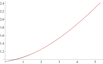
Figure 13: Fit of $B^{(3)}_{n}$ versus $x=\ln n$, using a function of the form (190).

However, we are not satisfied. We want to fit the value of $\alpha$, instead of trying up the predicted value (and, on top of this, with so many free parameters).

At this point we perform a further manipulation, and produce the series

$$C_{n}=\frac{B^{(3)}_{2n}}{B^{(3)}_{n}}\,.$$ (191)

Under the assumption that $B_{n}$ has no periodic behaviour (a fact that can be consistently checked numerically on the data), this further manipulation allows to further highlight the residual dependence from $n$. That is, a function of the form (188), in which we keep as parameters $\alpha$ and the first $k$ of the $a_{i}$’s.

For $k\leq 1$ the fit does not converge. For $k=2$ and $k=3$ the fitted values of $\alpha$ are $\alpha=1.84\ldots$ and $\alpha=1.98\ldots$, respectively. For $k\geq 4$ the proliferation of fit parameters, and their high covariance, make the fit less reliable. We suppose that the incredibly good value at $k=3$ is merely accidental, but the fact that these values are reasonably near to $2$ (and definitely off from 0) is a validation of the theoretical prediction. In figure 14 we show the fit of the data with functions at $k=2$ and $k=3$, as a function of $x=\ln 2/\ln n$.

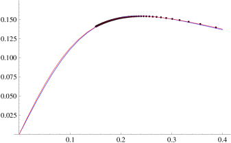
Figure 14: Fit of $C_{n}$ versus $x=\ln 2/\ln n$, using the ratio of functions of the form (190), with $k$ correction terms, evaluated at $2n$ (numerator) and at $n$ (denominator). Blue and red correspond to $k=2$ and $k=3$ respectively.

7 Conclusions

As we have discussed above, there is an increasing evidence that the model of spanning forests on random planar graphs of fixed degree shows the KPZ counterpart of a Berker–Kadanoff phase on an interval $(t_{\ast},0]$ of fugacities, with $t_{\ast}$ being negative and finite. In particular, at $t=0$ we have the well-known theory of spanning trees, which has string susceptibility exponent $\gamma=-1$, corresponding to a value $c=-2$. For negative values of $t$, up to the values $t_{\ast}$ discussed in Section 4, the string susceptibility remains $\gamma=-1$, while it develops logarithmic corrections, with exponent $\gamma^{\prime}=-2$. This is consistent with the value $c=-2$ found for spanning forests on flat lattices in [12]. Therefore the picture we (and previous literature [35]) have for spanning forests on random geometries, the KPZ relation, and the understanding of the Berker–Kadanoff phase in flat geometry all combine consistently. Outside this range of $t$, the theory is massive, with the possible exception of the theory at $t_{\ast}$, which may (and shall) be a non-trivial CFT, either with vanishing central charge, as follows from formula (84), or a non-unitary CFT with a value of $h_{\rm min}$ resulting into $\gamma=-1/2$, namely $h_{\rm min}=c/25$.

So, is everything unraveled?

In our perspective, this is not the case. There are various aspects of the phase diagram of this model — and also of its counterpart in regular lattices — which are not clear, and deserve further investigation.

One of these aspects is the origin of the logarithmic corrections (also in their regular counterpart). A satisfactory understanding would require to elucidate the features of logarithmic CFTs coupled to Liouville gravity, a topic that unfortunately, as far as we know, has never been addressed in the literature.

A second aspect, discussed in the conclusions of [8], is the combinatorial nature of the criticality in the Berker–Kadanoff phase. It is conjectured there that in this phase there is one tree occupying a finite fraction of the lattice, although this fact is hard to investigate theoretically or numerically, because of the lack of positivity in the Boltzmann weights. This problem may be easier to approach in the gravitational counterpart, especially in the cubic case, where we have an explicit expression for the spectral density.

A third aspect is the nature of criticality at $t_{\ast}$. Indeed, at discrepancy with [8], we do not see the counterpart of the theory with $c=-1$, consisting of symplectic fermions and one non-compact boson (unless somehow this theory has an unlikely field of lowest conformal dimension $h=-1/25$, compatible with the string susceptibility we find at $t_{\ast}$). As a less fundamental discrepancy, we do not see any relevant critical behaviour occurring in the case of vanishing monomer weight, in the formulation of the model as a gas of O$(-2)$ loops and dimers, as is the case in [8] for the regular square grid, so this may be an accident of that lattice.

Another issue is the comprehension of the massive phase below $t_{\ast}$ for quartic graphs, at the same level as done for cubic graphs. And an obvious issue is how to make rigorous the present derivation, in the regime $t<-1$.

Finally, it would be highly interesting to investigate the antiferromagnetic regime of the Potts model on random planar graphs beyond the case of spanning forests. A particularly interesting aspect is the behavior for $q$ a Beraha number, i.e. for $q=4\cos^{2}(\pi/\delta)$, $\delta\in\mathbb{N}$. At these values of $q$, the partition function of the $q$-state Potts model in the Berker–Kadanoff phase on flat lattices develops severe singularities, whose resolution is, to the best of our knowledge, only partially understood [6, 7, 9]. (See also [70] for a discussion of the Berker–Kadanoff phase for other graphs than the triangular and square lattice.) Nonetheless, it is conceivable that at least the critical indices computed for generic $\delta\geq 2$ continue to hold even at the Beraha numbers, as it appears to be the case for $\delta=2$, which corresponds to spanning forests. The quantum gravity counterpart of these and related issues may be clarified by ongoing work of Bernardi and Bousquet-Mélou, as continuation of [71, 72].

We hope to address some of the questions outlined above in future work.

References

- [1] W. Tutte, Graph Theory. Cambridge University Press, 2001.
- [2] A. D. Sokal, The multivariate Tutte polynomial (alias Potts model) for graphs and matroids, in Surveys in Combinatorics, B. S. Webb, ed., pp. 173–226. Cambridge University Press, 2005
- [3] S. Caracciolo, J. L. Jacobsen, H. Saleur, A. D. Sokal, and A. Sportiello, Fermionic field theory for trees and forests, Phys. Rev. Lett. 93 (2004) 080601.
- [4] C. De Grandi, S. Caracciolo, and A. Sportiello, Renormalization flow for unrooted forests on a triangular lattice, Nucl. Phys. B 787[FS] (2007) 260–282.
- [5] R. Baxter, Exactly Solved Models in Statistical Mechanics. Dover Publications, 2007.
- [6] H. Saleur, Zeroes of chromatic polynomials: a new approach to Beraha conjecture using quantum groups, Commun. in Math. Phys. 132 no. 3, (1990) 657–679.
- [7] H. Saleur, The antiferromagnetic Potts model in two dimensions: Berker-Kadanoff phase, antiferromagnetic transition, and the role of Beraha numbers, Nucl. Phys. B 360 no. 2, (1991) 219–263.
- [8] J. L. Jacobsen and H. Saleur, The arboreal gas and the supersphere sigma model, Nucl. Phys. B 716 no. 3, (2005) 439–461.
- [9] J. L. Jacobsen and H. Saleur, The antiferromagnetic transition for the square lattice Potts model, Nucl. Phys. B 743 (2006) 207–248.
- [10] J. L. Jacobsen, J. Salas, and A. D. Sokal, Transfer Matrices and Partition Function Zeros for Antiferromagnetic Potts Models. III. Triangular-Lattice Chromatic Polynomial, J. Stat. Phys. 112 no. 5, (2003) 921–1017.
- [11] E. Vernier, J. L. Jacobsen and J. Salas, Q-colourings of the triangular lattice: exact exponents and conformal field theory, J. Phys. A: Math. Theor. 49 no. 17 (2016): 174004.112.
- [12] J. L. Jacobsen, J. Salas, and A. D. Sokal, Spanning Forests and the -State Potts Model in the Limit , J. Stat. Phys. 119 no. 5, (2005) 1153–1281.
- [13] P. Di Francesco, P. H. Ginsparg, and J. Zinn-Justin, 2-D Gravity and random matrices, Phys. Rept. 254 (1995) 1–133.
- [14] P. Di Francesco, 2D quantum gravity, matrix models and graph combinatorics, in Application of random matrices in physics. Proceedings, NATO Advanced Study Institute, Les Houches, France, June 6-25, 2004, pp. 33–88. 2004.
- [15] B. Eynard, T. Kimura, and S. Ribault, Random matrices, arXiv e-prints (Oct. 2015), arXiv:1510.04430 [math-ph].
- [16] M. Bousquet-Mélou, Counting planar maps, coloured or uncoloured, in 23rd British Combinatorial Conference, vol. 392, pp. 1–50. 2011.
- [17] V. G. Knizhnik, A. M. Polyakov, and A. B. Zamolodchikov, Fractal structure of 2d-quantum gravity, Mod. Phys. Lett. A3 (1988) 819–826.
- [18] F. David, What is the intrinsic geometry of two-dimensional quantum gravity?, Nucl. Phys. B 368 no. 3, (1992) 671–700.
- [19] B. Duplantier and S. Sheffield, Liouville quantum gravity and KPZ, Invent. Math. 185 no. 2, (2011) 333–393.
- [20] F. David, A. Kupiainen, R. Rhodes, and V. Vargas, Liouville quantum gravity on the Riemann sphere, Commun. in Math. Phys. 342 no. 3, (2016) 869–907.
- [21] G. Schaeffer, Conjugaison d’arbres et cartes combinatoires aléatoires. PhD thesis, 1998.
- [22] M. Marcus and G. Schaeffer, Une bijection simple pour les cartes orientables, (2001) https://hal.inria.fr/inria-00100704/en.
- [23] G. Chapuy and M. Dołȩga, A bijection for rooted maps on general surfaces, arXiv e-prints (Jan. 2015), arXiv:1501.06942
- [24] J. Bouttier, P. Di Francesco, and E. Guitter, Census of planar maps: from the one-matrix model solution to a combinatorial proof, Nucl. Phys. B 645 no. 3, (2002) 477–499.
- [25] J. Bouttier, P. Di Francesco, and E. Guitter, Planar maps as labeled mobiles, Electron. J. Combin 11 no. 1, (2004) R69.
- [26] J. Bouttier and E. Guitter, Planar Maps and Continued Fractions, Commun. in Math. Phys. 309 no. 3, (2012) 623–662.
- [27] V. Kazakov, Exactly solvable Potts models, bond-and tree-like percolation on dynamical (random) planar lattice, Nucl. Phys. B Proc. Suppl. 4 (1988) 93–97.
- [28] O. Bernardi, A characterization of the Tutte polynomial via combinatorial embeddings, Ann. Comb. 12 no. 2, (2008) 139–153.
- [29] O. Bernardi and M. Bousquet-Mélou, Counting colored planar maps: algebraicity results, Journ. of Combin. Theory, Series B 101 no. 5, (2011) 315–377.
- [30] O. Bernardi, Counting coloured planar maps: differential equations, arXiv e-print (July 2015), arXiv:1507.02391
- [31] S. Caracciolo, A. D. Sokal, and A. Sportiello, Spanning forests and -invariant -models, to be published in this same issue (2016).
- [32] S. Caracciolo and A. Sportiello, Spanning Forests on Random Planar Lattices, J. Stat. Phys. 135 (2009) 1063–1104.
- [33] I. K. Kostov, Vector Model on a Planar Random Lattice: Spectrum of Anomalous Dimensions,Mod. Phys. Lett. A 04 no. 03, (1989) 217–226.
- [34] M. Gaudin and I. Kostov, model on a fluctuating planar lattice. Some exact results,Phys. Lett. B 220 no. 1, (1989) 200–206.
- [35] M. Bousquet-Mélou and J. Courtiel, Spanning forests in regular planar maps, Journ. of Combin. Theory, Series A 135 (2015) 1–59.
- [36] I. Kostov and M. Staudacher, Multicritical Phases of the model on a Random Lattice, Nucl. Phys. B 384 (1992) 459–483.
- [37] J. Courtiel, Combinatoire du polynôme de Tutte et des cartes planaires, PhD Thesis, arXiv e-prints (Nov. 2014), arXiv:1411.0737 [math.CO].
- [38] G. Borot, J. Bouttier, and E. Guitter, A recursive approach to the model on random maps via nested loops, J. Phys. A: Math. and Theor. 45 no. 4, (2011) 045002.
- [39] G. Borot, J. Bouttier, and E. Guitter, More on the model on random maps via nested loops: loops with bending energy, J. Phys. A: Math. and Theor. 45 no. 27, (2012) 275206.
- [40] G. Borot, J. Bouttier, and E. Guitter, Loop models on random maps via nested loops: the case of domain symmetry breaking and application to the Potts model, J. Phys. A: Math. and Theor. 45 no. 49, (2012) 494017.
- [41] R. L. Graham, D. E. Knuth and O. Patashnik, Concrete Mathematics: A Foundation for Computer Science. Addison-Wesley Longman Publishing Co., Inc., 1994.
- [42] B. Nienhuis, Exact critical point and critical exponents of O(n) models in two dimensions, Phys. Rev. Lett. 49 no. 15, (1982) 1062.
- [43] C. M. Yung and M. T. Batchelor, Integrable vertex and loop models on the square lattice with open boundaries via reflection matrices, Nucl. Phys. B 435 no. 3, (1995), Pages 430-462.
- [44] G. Borot and B. Eynard, Enumeration of maps with self-avoiding loops and the model on random lattices of all topologies, J. Stat. Mech 2011 no. 01, (2011) P01010.
- [45] G. Borot, B. Eynard, and N. Orantin, Abstract loop equations, topological recursion and new applications, Commun. Num. Theor. Phys. 09 (2015) 51–187.
- [46] M. Staudacher, The Yang-Lee edge singularity on a dynamical planar random surface, Nucl. Phys. B 336 no. 3, (1990) 349–362.
- [47] S. Caracciolo, A. D. Sokal, and A. Sportiello, Grassmann integral representation for spanning hyperforests, J. Phys. A: Math. and Theor. 40 no. 46, (2007) 13799.
- [48] F. Gakhov, Boundary Value Problems. Dover books on advanced mathematics. Dover, 1990.
- [49] J. Bouttier, Matrix integrals and enumeration of maps, chapter of The Oxford Handbook of Random Matrix Theory, eds. G. Akemann, J. Baik and P. Di Francesco, (2011).
- [50] I. K. Kostov, Exact solution of the three-color problem on a random lattice, Phys. Lett. B 549 no. 1–2, (2002) 245–252.
- [51] I. K. Kostov, Exact solution of the six-vertex model on a random lattice, Nucl. Phys. B 575 no. 3, (2000) 513–534.
- [52] P. Zinn-Justin, The six-vertex model on random lattices, EPL (Europhysics Letters) 50 no. 1, (2000) 15.
- [53] J. Ambjørn, T. Budd, and Y. Makeenko, Generalized multicritical one-matrix models, arXiv e-print (Apr. 2016), arXiv:1604.04522
- [54] P. Flajolet and R. Sedgewick, Analytic Combinatorics. Cambridge University Press, 2009.
- [55] E. Brézin, M. R. Douglas, V. Kazakov, and S. H. Shenker, The Ising model coupled to 2D gravity. A nonperturbative analysis, Phys. Lett. B 237 no. 1, (1990) 43–46.
- [56] H. Saleur, Polymers and percolation in two dimensions and twisted supersymmetry, Nucl. Phys. B 382 no. 3, (1992) 486–531.
- [57] E. V. Ivashkevich, Correlation functions of dense polymers and conformal field theory, J. Phys. A: Math. and Gen. 32 no. 9, (1999) 1691.
- [58] I. Affleck, D. Gepner, H. Schulz, and T. Ziman, Critical behaviour of spin-s Heisenberg antiferromagnetic chains: analytic and numerical results, J. Phys. A: Math. and Gen. 22 no. 5, (1989) 511.
- [59] E. Brézin, V. Kazakov, and A. Zamolodchikov, Scaling violation in a field theory of closed strings in one physical dimension, Nucl. Phys. B 338 no. 3, (1990) 673–688.
- [60] I. Gradshtein, I. Ryzhik, D. Zwillinger, and I. S. Technica, Table of Integrals, Series, and Products. Academic Press, 2014.
- [61] W. H. Mills, D. P. Robbins, and H. Rumsey, Alternating sign matrices and descending plane partitions, Journ. of Combin. Theory, Series A 34 no. 3, (1983) 340–359.
- [62] O. Bernardi, A Characterization of the Tutte Polynomial via Combinatorial Embeddings, Ann. Comb. 12 no. 2, (2008) 139–153.
- [63] S. Sheffield, Quantum gravity and inventory accumulation, arXiv e-print arXiv:1108.2241 (2011), to be published in Annals of Prob.
- [64] L. Chen, Basic properties of the infinite critical-FK random map, arXiv e-print (Feb. 2015), arXiv:1502.01013
- [65] N. Berestycki, B. Laslier, and G. Ray, Critical exponents on Fortuin–Kastelyn weighted planar maps, arXiv e-print (Feb. 2015), arXiv:1502.00450
- [66] A. Kassel and D. B. Wilson, Active spanning trees and Schramm-Loewner evolution, arXiv e-prints (Dec. 2015), arXiv:1512.09122 [cond-mat.stat-mech].
- [67] E. Gwynne, A. Kassel, J. Miller, and D. B. Wilson, Active spanning trees with bending energy on planar maps and SLE-decorated Liouville quantum gravity for , arXiv e-prints (Mar. 2016), arXiv:1603.09722 [math.PR].
- [68] A. J. Guttmann and G. S. Joyce, On a new method of series analysis in lattice statistics, J. Phys. A: Gen. Phys. 5 no. 9, (1972) L81.
- [69] C. Domb, M. Green, and J. Lebowitz, Phase transitions and critical phenomena. No. v. 13 in Phase Transitions and Critical Phenomena. Academic Press, 1989.
- [70] J. L. Jacobsen, High-precision percolation thresholds and Potts-model critical manifolds from graph polynomials, J. Phys. A: Math. Theor. 47 no. 13 (2014): 135001.
- [71] O. Bernardi and M. Bousquet-Mélou, Counting colored planar maps: algebraicity results., Journ. of Combin. Theory, Series B 101 no. 5, (2011) 315–-377.
- [72] O. Bernardi and M. Bousquet-Mélou, Counting coloured planar maps: differential equations, arXiv e-prints (Jul. 2015), arXiv:1507.02391 [math.CO].