Magnetic Order and Mott Transition on the Checkerboard Lattice

Abstract

The checkerboard lattice, with alternating ‘crossed’ plaquettes, serves as the two dimensional analog of the pyrochlore lattice. The corner sharing plaquette structure leads to a hugely degenerate ground state, and no magnetic order, for classical spins with short range antiferromagnetic interaction. For the half-filled Hubbard model on this structure, however, we find that the Mott insulating phase involves virtual electronic processes that generate longer range and multispin couplings. These couplings lift the degeneracy, selecting a ‘flux like’ state in the Mott insulator. Increasing temperature leads, strangely, to a sharp crossover from this state to a ‘120 degree’ correlated state and then a paramagnet. Decrease in the Hubbard repulsion drives the system towards an insulator-metal transition - the moments reduce, and a spin disordered state wins over the flux state. Near the insulator-metal transition the electron system displays a pseudogap extending over a large temperature window.

1 INTRODUCTION

Frustrated magnets arise due to the coupling between electrons localised on non bipartite lattices [1, 2, 3]. The localisation stems from electron correlation, a concrete example being the Mott insulating phase of the half filled Hubbard model [4]. The $U/t\gg 1$ limit in such cases, where $U$ is the Hubbard repulsion and $t$ the typical kinetic scale, involves virtual hopping of the electrons, and induces antiferromagnetic exchange. With weakening $U/t$ the electrons ‘delocalise’ over progressively longer distance and mediate longer range couplings [5, 6]. These additional couplings are crucial in deciding the physics when the $U/t\gg 1$ Heisenberg limit involves a macroscopically degenerate ground state. The checkerboard lattice, Fig.1, is in this category [7].

Two complications arise with decreasing $U/t$: (a) the size of the moments diminish as the system heads towards the Mott transition, and (b) the range of electron hops increase and the exchange processes get harder to quantify. Near the insulator-metal transition (IMT) the magnetic correlations on the frustrated lattice, and their impact on electronic properties, have to be worked out self-consistently. This has indeed been attempted for various frustrated lattices, e.g, the edge-shared triangular [8, 9, 10, 11, 12, 13] and FCC [14, 15, 16] lattices, the corner shared kagome [17, 18] and pyrochlore [19, 20] lattices. Surprisingly, very little attention has been given to the frustrated checkerboard latice.

For the checkerboard lattice the Heisenberg antiferromagnet is well understood [7, 21, 22, 23, 24, 25, 26, 27, 28, 29, 30]. The classical ground state is macroscopically degenerate [7] and there is no order at any temperature. The quantum, $S=1/2$, case is argued to be a plaquette valence-bond crystal [21, 22, 23, 24, 25, 26, 27, 28, 29, 30] - the product of singlets on the uncrossed plaquettes.

There is limited work on the checkerboard Hubbard model, focused mainly on the ground state. One study [31] suggested that increasing $U/t$ leads to a transition from the semi-metallic band state to a charge-ordered insulator, and then to a magnetically disordered Mott insulator, while another reports a first order transition from the semi-metal to an insulating state with plaquette magnetic order [32].

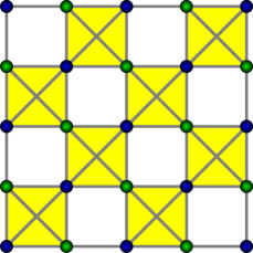
Figure 1: Color online: The checkerboard lattice with alternating ‘empty’ and crossed plaquettes. All hopping amplitudes (diagonal and axial) are equal. The structural unit cell contains two atoms. Each crossed plaquette, in isolation, can be viewed as a tetrahedron.

The varying results, based on different methods [31, 32, 33], leave some questions unanswered: (i) What magnetic ground state emerges within a Hartree-Fock (HF) scheme, non trivial here since the HF state may be disordered. (ii) What are the effects of thermal fluctuation on this magnetic state? and (iii) What is the impact of the magnetic order, and fluctuations, on the electronic properties near the IMT? We address these questions using a combination of Hartree-Fock theory for the ground state and an auxiliary field based Monte Carlo to handle thermal fluctuations. Our results reveal a wide variety of magnetic and spectral regimes on this lattice, summarised below.

(1). Strong coupling: Deep in the Mott phase the Hubbard model selects out a flux like state from the infinitely degenerate manifold of the checkerboard Heisenberg model. This persists as the low temperature state down to $U\sim 5.3t$. Increasing temperature promotes a $120$ degree spin arrangement, before the final loss of order. (2). Weak coupling: Small disordered moments persist below the insulator-metal transition (at $U\sim 5.3t$) down to $U\sim 3t$. (3). Electronic state: The electrons are gapped in the flux phase, but the crossover to the $120$ degree state leads to a reduction of the gap. As $U/t$ reduces, the $120$ degree phase becomes pseudogapped.

2 MODEL AND METHOD

We consider the single band Hubbard model on the checkerboard lattice,

$$H=\sum_{ij,\sigma}(t_{ij}-\mu\delta_{ij})c_{i\sigma}^{\dagger}c_{j\sigma}+U\sum_{i}n_{i\uparrow}n_{i\downarrow}$$

$t_{ij}=-t$ for the nearest neighbour (NN) axial as well as diagonal bonds. $U>0$ is the interaction strength and $\mu$ is chosen to keep the system at electron density $n=1$. We set $t=1$ and measure all energies in this unit.

We follow an approach originally suggested by Hubbard [34] to obtain a rotation invariant auxiliary field decomposition [35, 36] of the interaction term. Retaining rotation invariance and reproducing Hartree-Fock theory at saddle point requires the introduction of a three dimansional auxiliary vector field, ${\vec{m}}_{i}(\tau)$, and a scalar field $\phi_{i}(\tau)$. We treat $\phi$ as independent of $i,\tau$ (as would happen at saddle point) while for ${\vec{m}}_{i}$ we retain the spatial fluctuations but not the imaginary time dependence. In this limit the partition function can be written in terms of the effective Hamiltonian [13]:

$$H_{eff}=\sum_{ij,\sigma}t_{ij}c_{i\sigma}^{\dagger}c_{j\sigma}-{\tilde{\mu}}N-{U\over 2}\sum_{i}{\vec{m}}_{i}.{\sigma}_{i}+\frac{U}{4}\sum_{i}\vec{m_{i}}^{2}$$

where $\tilde{\mu}=\mu-(U/2)$ and ${\vec{\sigma}}_{i}$ is the electron spin operator. The distribution function of the $\{{\vec{m}}_{i}\}$ is obtained by tracing over the fermions:

$$P\{{\vec{m}}_{i}\}\sim Tr_{c,c^{\dagger}}e^{-\beta H_{eff}\{{\vec{m}}_{i}\}}$$

with $\beta=1/(k_{B}T)$, where $T$ is the temperature and we set $k_{B}=1$. The equations for $H_{eff}$ and $P\{{\vec{m}}_{i}\}$ define a self-consistent loop.

To gain some insight it is helpful to separate three regimes. (1) As $T\rightarrow 0$ the problem reduces to minimising the energy of $H_{eff}$ with respect to the ${\vec{m}}_{i}$. The minimisation is equivalent to the HF condition ${\vec{m}}_{i}=\langle{\vec{\sigma}}_{i}\rangle$. So at $T=0$ this approach just reproduces mean field theory (without any assumption, however, about the spatial organisation of the ${\vec{m}}_{i}$). (2) At low finite $T$, the crucial low energy angular fluctuations of ${\vec{m}}_{i}$ come into play, revealing the thermal correlation scale of the moments. (3) At high $T$, where the ${\vec{m}}_{i}$ are essentially random, the auxiliary field mimics the effect of electron-electron interaction mainly by preventing double occupancy in the large $U/t$ regime.

We use two approaches to study $H_{eff}$. (i) At finite $T$ we use a Monte Carlo (MC) approach, using a cluster algorithm [37] to generate equilibrium configurations of the ${\vec{m}}_{i}$. We typically use a $N=24\times 24$ lattice with $8\times 8$ update clusters. We anneal down from $T=0.1t$ (since we see no correlations above that temperature) and use $10^{4}$ MC sweeps per temperature, going down to $T=10^{-4}t$. Physical properties are averaged over $\sim 100$ configurations at each $T$. (ii) At $T=0$ we use a variational scheme, trying out a family of periodic ${\vec{m}}_{i}$ configurations (both planar and non-planar) and cross check our results with the Monte Carlo based annealing of the ${\vec{m}}_{i}$.

To characterise the magnetic state we calculate the following indicators with the equilibrium MC configurations.

$$S(\vec{q}) = \frac{1}{N^{2}}\sum_{ij}\langle\vec{m_{i}}.\vec{m_{j}}\rangle e^{i\vec{q}\cdot(\vec{R_{i}}-\vec{R_{j}})}$$ (1)

$$\tau_{avg} = \frac{1}{N}\sum_{i}\int_{0}^{t_{max}}dt^{\prime}\langle\vec{m_{i}}(0).\vec{m_{i}}(t^{\prime})\rangle$$ (2)

$$P(m) = \frac{1}{N}\sum_{i}\langle\delta(m-|{\vec{m}}_{i}|)\rangle$$

In the expressions above $N$ is the system size and the angular brackets stand for thermal average. In sequence, (i) $S(\vec{q})$ is the thermally averaged magnetic structure factor. The onset of rapid growth in $S(\vec{q})$ at some wavevector $\vec{Q}$ indicates magnetic ordering. In the thermodynamic limit, there would be no ‘true’ long-range magnetic ordering at finite temperature in two dimensions (2D). Our magnetic orders refer to growing magnetic correlation length scales beyond system sizes. We have checked the size dependence of the various temperature scales associated with these crossovers within the MC. Our MC runs on $16\times 16$, $24\times 24$ and $32\times 32$ lattices show that the characteristic temperature scales reduce very slowly with increasing size. (ii) To consider the possibility of freezing without long range order we compute a MC based ‘relaxation time’ [38] $\tau_{avg}$ where $t_{max}\sim 10^{4}$ steps and $t^{\prime}$ is the MC ‘time’. If on lowering the temperature, the system undergoes a magnetic ordering transition, then there is a rapid growth in $\tau_{avg}$ accompanied by a growth in the structure-factor at the wavevector $\vec{Q}$. The case where one observes a rapid growth in $\tau_{avg}$ but not in the structure-factor at any $\vec{Q}$, suggests a glass transition [38]. (iii) The distribution of the magnitude of the auxiliary moments is given by $P(m)$. Since the presence of a gap in the electronic density of states depends on the typical size of the ${\vec{m}}_{i}$, $P(m)$ is an important input in inferring transport. The mean moment $m_{avg}=\int mP(m)dm$.

The overall electronic density of states (DOS) can be calculated from the single particle eigenvalues, $\epsilon_{n}$, in the equilibrium configurations, as:

$$D(\omega)=\frac{1}{N}\sum_{n}\langle\delta(\omega-\epsilon_{n})\rangle$$

3 RESULTS

3.1 Ground state

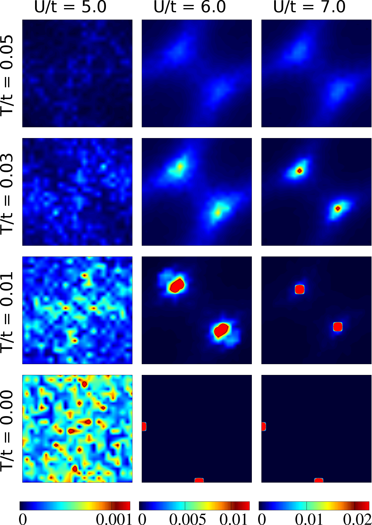
Figure 2: Color online: Magnetic structure factor $S(\vec{q})$ over $q_{x}$, $q_{y}$ $\in$ $[0,2\pi]$ for different temperature and interaction strengths. The value of $S(\vec{q})$ follows the color code. The left column, at $U=5t$ has no prominent peaks at any temperature, indicating a short range correlated state. The middle and right columns have distinct peaks at $T=0$, at locations corresponding to flux-like state, but the peak location shifts to that of a $120$ degree correlated state at a small finite temperature.

Let us focus on the low temperature result, at $T\sim 10^{-4}t$, obtained via a MC on lowering $T$. We label this as $T=0$ in the lowest row in Fig.2, which shows the structure factor versus $q_{x}$ and $q_{y}$. The leftmost panel, typical of the window $3t<U<5.3t$, show no prominent features in the structure factor. It is suggestive of local moments with weak and short range correlations. We will need to look at the local moment magnitudes to fully characterise this window. For $U\geq 5.3t$ the structure factor shows distinct peaks at $\vec{Q_{F_{1}}}=$ ($\pi$,0) and $\vec{Q_{F_{2}}}=$ (0,$\pi$) with the weight at peak position increasing initially with $U/t$ and saturating for $U/t\geq 10$. We call this the ‘flux’ phase. The real space arrangement of the spins in the ‘flux’ phase is shown in the lower panel in Fig.3.

In our MC runs, we obtain the ‘flux’ state at the lowest temperature only in a small window of interaction strength, $U=[5.3t,5.7t]$, near the IMT. The system encounters a ‘120 degree’ spin arrangement when cooled from high temperature, and does not manage to transit to the flux state, despite the flux state having the lowest ground state energy for all $U/t\geq 5.3$. On heating up from the flux state the order survives to a low finite $T$ and then the system enters the 120 degree phase. We will discuss the results of the variational approach and its consistency with the MC results further on.

3.2 Finite temperature correlations

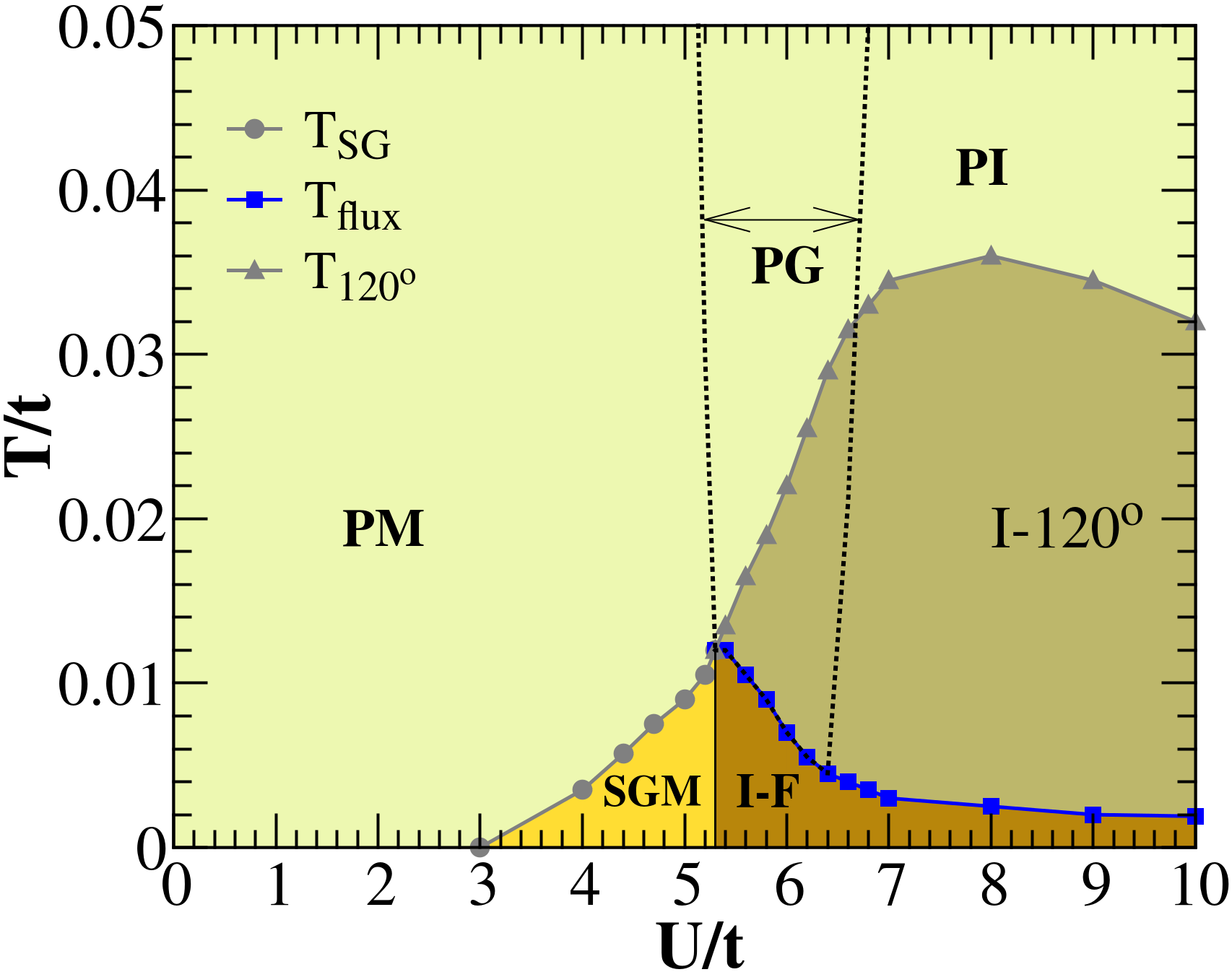
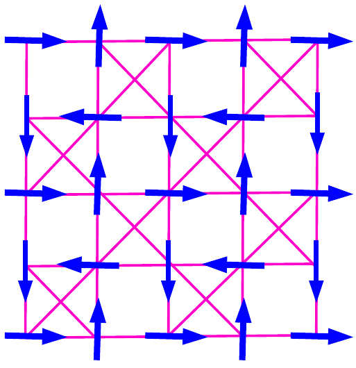
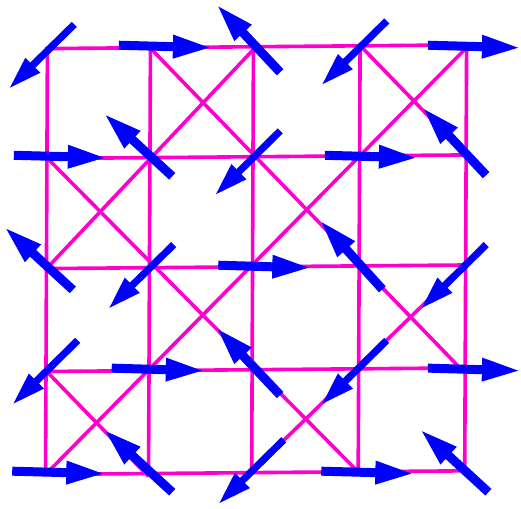
Figure 3: Color online: Top: The phase diagram of the checkerboard Hubbard model at half-filling. The ground state is a paramagnetic metal (PM) for $U\leq 3t$, a spin glass metal (SGM) for $3t<U<5.3t$, and an insulator with ‘flux’ like correlations (I-F) for $U\geq 5.3t$. With increase in temperature, the ‘flux’ correlated phase transforms to a $120$ degree correlated state (I-$120^{o}$) and then to the paramagnet (PI). The $120$ degree phase is gapped, except for $5.3t\leq U\leq 6.5t$, near the insulator-metal transition, where it shows a pseudogap (PG). The different temperature scales shown in this panel correspond to magnetic correlation length growing beyond system size. These temperature scales are crossover scales from one magnetic phase to another. $T_{SG}$ represents a crossover from a PM to a SGM phase, $T_{flux}$ represents a crossover from flux phase to $120$ degree phase and $T_{120^{o}}$ refers to a crossover from $120$ degree state to a paramagnet. Bottom: A schematic of the ‘flux’ phase (left) and the 120 degree phase (right) on the checkerboard lattice.

There are four broad coupling regimes in terms of temperature effects. The data in Fig.2 is for the two central regimes, but we discuss all the four regimes below.

(i) At very weak coupling, $U<3t$, there are no local moments in the ground state. Increasing temperature generates small moments but there are no significant spatial correlations between them. Since this state is fairly obvious we have not included the result for this regime in Fig.2.

(ii) At somewhat larger couplings, $3t<U<5.3t$, there are disordered moments in the ground state. These moments seem to be frozen on the basis of $\tau_{avg}$ estimates and the frozen state survives to a ‘spin-glass temperature’ $T_{SG}$. The left column in Fig.2 shows the $T$ dependence of magnetic structure factor, $S({\vec{q}})$ in this coupling window. It is clearly seen that $S({\vec{q}})$ is featureless in this regime.

(iii) For larger interaction strength, $U\sim[5.3t,8t]$, $S({\vec{q}})$ shows peaks at wavevectors $\vec{Q_{F_{1}}}=(\pi,0)$ and $\vec{Q_{F_{2}}}=(0,\pi)$ in the ground state. We call this the ‘flux’ phase. The amplitude at these wavevectors decrease with increasing $T$ and beyond a scale $T=T_{flux}$ new peaks appear at $\vec{Q_{T_{1}}}=(\pi/3,2\pi/3)$ and $\vec{Q_{T_{2}}}=(2\pi/3,\pi/3)$. These peaks correspond to a $120$ degree arrangement of the moments. This is visible in the middle and right columns in Fig.2. The weights at the ${\vec{Q}}_{T}$ increase quickly with temperature, reach a maximum, and then decrease - vanishing at $T=T_{120^{o}}$. For $T>T_{120^{o}}$ there is no peak in $S(\vec{q})$ for any $\vec{q}$, indicating the paramagnetic regime. In this $U/t$ window $T_{120^{o}}$ increases with increasing $U$.

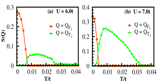
Figure 4: Color online: Variation of structure factor peak amplitude at the flux wavevector $\vec{Q_{F_{1}}}=(\pi,0)$ and the triangular arrangement wavevector $\vec{Q_{T_{1}}}=(\pi/3,2\pi/3)$ with temperature.

(iv) In the asymptotically large coupling regime, $U\gtrsim 8t$, the same sequence of flux and $120$ degree correlations are obtained with increasing temperature, but the characteristic $T$ scales fall with increasing $U/t$.

The top panel in Fig.3 shows the phase diagram based on the $S({\vec{q}})$. Fig.4 shows the $T$ dependence of the structure factor peak, highlighting the multiple thermal crossovers observed within our MC. Here $S(\vec{Q_{F_{1}}})$ corresponds to the structure factor for flux like order, whereas $S(\vec{Q_{T_{1}}})$ corresponds to the structure factor for ‘$120$ degree’ like order.

3.3 Local moment distribution

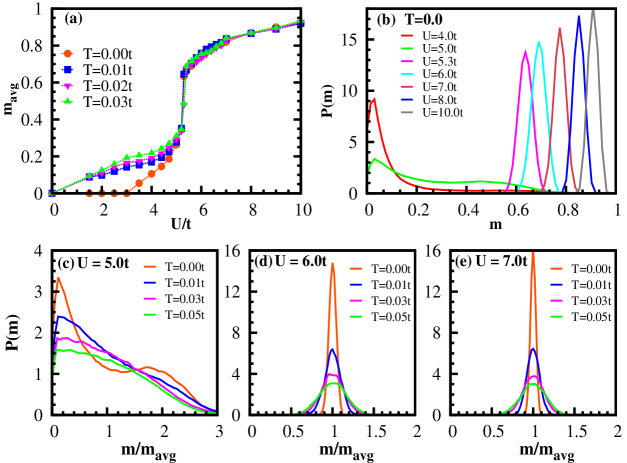
Figure 5: Color online: (a) Temperature dependence of average local moment $m_{avg}$ with $U/t$. (b) $P(m)$ in the ground state for varying $U/t$. (c)-(e) Temperature dependence of $P(m)$ for $U/t=5.0,~{}6.0,~{}7.0$.

Fig.5(a) shows the behavior of the mean local moment magnitude $m_{avg}$ with interaction strength. In the ground state, there is no local-moment for $U\leq U_{c1}\sim 3t$. There is a small average moment for $U_{c1}\leq U<U_{c2}\sim 5.3t$. The average moment increases with interaction strength in the $[U_{c1},U_{c2}]$ window but for $U=U_{c2}$ there is a jump in the average moment value. The average moment again increases slowly for $U>U_{c2}$ and saturates to $m_{avg}=1.0$ as $U/t\rightarrow\infty$.

With increase in temperature there are both orientational and magnitude fluctuations in the moments. Though the average moment remains unchanged in the strong interaction side, it shows significant changes in the weak interaction side due to the small amplitude stiffness.

Fig.5(b) shows the $P(m)$ for the ground state. This evolves from a broad distribution in the spin glass window to essentially a delta function in the Mott phase. To get a feel for the thermal fluctuations at different interaction strengths we have plotted the $P(m)$ vs $m/m_{avg}$ for $U=5t,~{}6t,~{}7t$ and different temperatures (Fig.5(c)-(e)). At $U=5t$ the distribution is already broad at $T=0$ due to the amplitude inhomogeneity in the glassy state. The low $T$ for which the data is shown does not lead to significant change. At $U=6t,~{}7t$ the $T=0$ result is essentially a delta function and it broadens slightly on raising temperature. On the strong coupling, Mott, side the dominant fluctuations are in the orientation of the moments, not their magnitude.

3.4 Insulator-metal transition

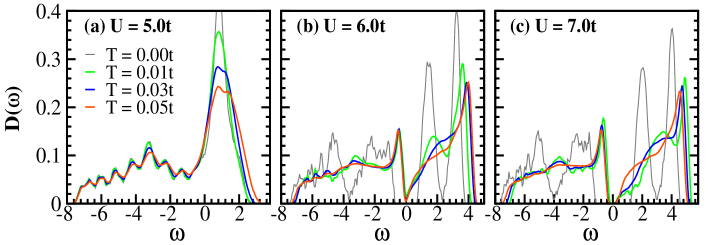
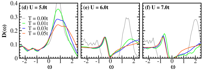
Figure 6: Color online: Electronic density of states (DOS) for $U/t=5.0,~{}6.0,~{}7.0$ and varying temperature. The upper row shows the DOS over a wide frequency window to emphasize its global features while the lower row shows the DOS over a much smaller frequency window centered on the Fermi level.

The first guess about the metallic or insulating behavior of the electrons can be made from the single particle density of states $D(\omega)$. Fig.6 shows the density of states for different $U/t$ and temperatures. For $U/t=5.0$ the ground state has small $m_{avg}$, $\approx 0.1$, and spatially disordered local moments. These local-moments are not large enough to open a gap at the Fermi energy. They broaden the flat tight-binding band, generating finite DOS at the Fermi energy. The system would be metallic in this regime. For $U/t=6.0$ the local-moments are sizable, $m_{avg}\approx 0.7$, large enough to open a gap in the DOS. Thus the system is insulating in this regime. With further increase in $U/t$, $m_{avg}$ increase monotonically saturating to $m_{avg}\approx 1.0$.

With increase in temperature the local moments fluctuate, both in amplitude and orientation. At weak coupling, $U<U_{c2}$, the small fluctuating moments broaden the DOS feature around $\omega=0$ maintaining the metallic nature. In the strong coupling side, $U/t>7.0$, the sizable moments maintain a gap in the DOS despite strong angular fluctuations. At intermediate coupling, $5.0<U/t<6.4$, the DOS shows a dip at $\omega=0$ without any clear gap. We call this ‘pseudogap’ (PG) phase. The PG feature survives upto very large temperature.

The metallic or insulating character should actually be inferred from a conductivity calculation. At large $U/t$ the presence of a gap is enough to ensure that the system would be insulating, without having to compute the conductivity. On the small $U/t$ side however, the situation is more complicated since we have a disordered situation in 2D. Since the disorder is weak and of a magnetic nature (rather than a scalar potential) we guess that spin flip scattering would sustain a metallic state.

4 DISCUSSION

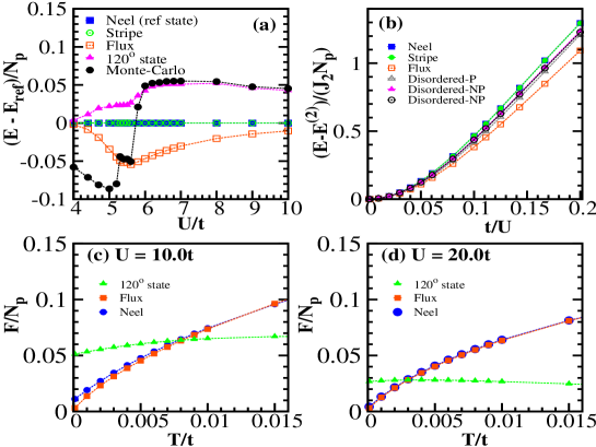
Figure 7: Color online: (a) Ground state energies of variational Neel, stripe, flux, the $120$ degree state, and the state obtained from Monte-carlo cooling. Energy of the Neel state is taken as the reference energy. (b) Energy due to the quartic hopping processes (leading $t^{4}/U^{3}$ corrections). The energy change of the Neel, $120$ degree state, and disordered zero-plaquette-spin configurations (planar and non-planar) are higher than the flux phase (they all have the same energy in the Heisenberg limit). (c)-(d) Free energy due to low-lying excitations on the variational Neel, flux, $120$ degree triangle states at two values of $U/t$. The methodology is explained in the text. Notice that the free energy of the $120$ degree state falls below that of the flux phase at a temperature that reduces with increasing $U/t$. $N_{p}$ is the number of plaquettes on the lattice.

4.1 Origin of the magnetic phases

Let us describe the variational scheme that we have used to complement the Monte Carlo and then move on to the analysis of the magnetic phases observed in Fig.2. We set up trial states using spiral spin configurations, ${\vec{m}}_{i}=m_{0}(cos(\vec{Q}.\vec{R_{i}}),sin(\vec{Q}.\vec{R_{i}}),0)$, with uniform magnitude $m_{0}$ and wave-vector $\vec{Q}$ as variational parameters, and minimised the energy of $H_{eff}$ at half-filling. This differs slightly from the real situation where the ${\vec{m}}_{i}$’s have some amplitude inhomogeneity. We also included several ‘non spiral’ configurations, notably the flux, that satisfy the local constraint of vanishing plaquette spin.

Comparing the minimum energy obtained via variational calculation with that from the MC cooling run, see Fig.7(a), confirms that the flux state is the ground state for $U\geq U_{c2}$. However the inhomogeneous small moment ‘spin glass’ phase obtained by our Monte-Carlo cooling indeed turns out to be the lowest energy state for $U_{c1}<U<U_{c2}$, lower than the trial periodic configurations.

How do we understand the magnetic phases? It is helpful to consider three separate regimes: (i) The $U/t\gg 1$ window where only the leading exchange term $J_{2}\sim t^{2}/U$ is relevant, and the moment size $m_{avg}\sim 1$. (ii) Intermediate $U/t$, down to $U\sim U_{c2}$, where the moment size is still large but higher order spin-spin couplings, in particular $J_{4}\propto t^{4}/U^{3}$, is significant. Finally (iii) the ‘weak coupling’ end, $U\sim 3t$, where the moment is small and it is more appropriate to expand about the band limit rather than the Mott state. Let us consider the ground state and thermal effects in succession.

Ground state: In the strong coupling limit, we can write an effective magnetic Hamiltonian on this lattice by tracing out the fermions order by order in $t/U$. This gives us

$$H_{eff}\{{\bf m}\} = E^{(2)}\{{\bf m}\}+E^{(4)}\{{\bf m}\}+...$$ (3)

(4)

$$E^{(2)}\{{\bf m}\} = J_{2}\sum_{\boxtimes}\sum_{\langle i,j\rangle}({\bf m}_{i}.{\bf m}_{j}-1)~{}~{}$$ (5)

$$E^{(4)}\{{\bf m}\} = E^{(4)}_{\boxtimes}\{{\bf m}\}+E^{(4)}_{coup}\{{\bf m}\}$$ (6)

(7)

$$E^{(4)}_{\boxtimes}\{{\bf m}\} = J_{4}\sum_{\boxtimes}[~{}~{}~{}\sum_{\langle i,j\rangle}\{\frac{5}{2}({\bf m}_{i}.{\bf m}_{j})^{2}-{\bf m}_{i}.{\bf m}_{j}-\frac{3}{2}\}$$ (8)

(9)

$$~{}~{}~{}~{}~{}~{}~{}~{}+\sum_{\langle i,j,k\rangle}\{5({\bf m}_{i}.{\bf m}_{j})({\bf m}_{j}.{\bf m}_{k})-3({\bf m}_{i}.{\bf m}_{k})\}$$ (10)

(11)

$$~{}~{}~{}~{}~{}~{}~{}~{}+\sum_{\langle i,j,k,l\rangle}\{5({\bf m}_{i}.{\bf m}_{j})({\bf m}_{k}.{\bf m}_{l})+5({\bf m}_{i}.{\bf m}_{l})({\bf m}_{j}.{\bf m}_{k})$$ (12)

(13)

$$~{}~{}~{}~{}~{}~{}~{}~{}~{}~{}~{}~{}~{}~{}~{}~{}~{}~{}~{}~{}+5({\bf m}_{i}.{\bf m}_{k})({\bf m}_{j}.{\bf m}_{l})\}]~{}~{}$$ (14)

$$E^{(4)}_{coup}\{{\bf m}\} \sim J^{\prime}_{4}\sum_{i\in\boxtimes_{1},j\in\boxtimes_{2}}{\bf m}_{i}.{\bf m}_{j}+J^{\prime\prime}_{4}\sum_{i\in\boxtimes_{1},j\in\boxtimes_{2}}^{k\in\boxtimes_{1}\cap\boxtimes_{2}}({\bf m}_{i}.{\bf m}_{k})({\bf m}_{j}.{\bf m}_{k})...$$

where $\boxtimes$ represents the crossed plaquette. $E^{(2)}\{{\bf m}\}$ corresponds to the second order perturbation energy with $J_{2}=t^{2}/U$, and $E^{(4)}\{{\bf m}\}$ corresponds to the fourth order perturbation energy. $E^{(4)}_{\boxtimes}$ describes the 4th order terms within a crossed-plaquette, while $E^{(4)}_{coup}$ describes the interplaquette terms with a common corner shared site. We have found  $J_{4}=\frac{t^{4}}{U^{3}}$ and $J^{\prime}_{4},J^{\prime\prime}_{4}\sim O(\frac{t^{4}}{U^{3}})$.

In regime (i), one would drop the $E^{(4)}\{{\bf m}\}$ term and obtain a classical Heisenberg model. On the checkerboard lattice the Heisenberg interaction can be written as the sum of squares of the total spin on each plaquette, ${\vec{S}}_{P}=\sum_{i}{\vec{m}}_{i}$, where the sum is over spins in individual crossed plaquettes. This feature arises due to the ‘fully connected’ nature of the crossed plaquettes, which are essentially tetrahedra, and is true of the pyrochlore lattice as well. The minimum energy corresponds to all ${\vec{S}}_{P}=0$ but there is a macroscopic degeneracy in the number of ways this can be satisfied. In such degenerate situations thermal fluctuations sometime select out collinear ordered configurations, due to the entropy gain [39]. For the checkerboard lattice it seems that free energy barriers are small and the thermal ‘order-by-disorder’ mechanism does not select out an ordered state. The classical Heisenberg limit, $U/t\rightarrow\infty$, is disordered at all temperatures as in the pyrochlore lattice [7]. For the Hubbard model the actual spins are $S=1/2$ and not classical, and a $1/S$ expansion about the classical limit suggests that a ‘quantum order by disorder’ mechanism selects a valence bond solid (VBS) ground state [40, 41, 42].

In regime (ii) the contribution of $E^{(4)}\{{\bf m}\}$ becomes important. This can be seen as follows. Various configurations satisfying the local constraint, $\sum_{i\in\boxtimes}{\bf m}_{i}=0$ have equal $E^{(2)}\{{\bf m}\}$. However the Hubbard energy for these different configurations are found to be different. Thus the crucial difference to the Hubbard energy is dominated by the $E^{(4)}\{{\bf m}\}$ contribution. We believe, these multi-spin exchange interactions are responsible in modifying the magnetic ground state away from the Heisenberg limit. In figure 7.(b), we show this contribution as $(E-E^{(2)}\{{\bf m}\})/J_{2}\approx(t/U)^{2}f({\bf m}_{i},{\bf m}_{j},{\bf m}_{k},{\bf m}_{l})$ with the expected quadratic behaviour as $t/U\rightarrow 0$ (or $U/t\rightarrow\infty$). Its also seen that the flux state has the largest lowering of energy to ${\cal O}(t^{4}/U^{3})$. This trend persists down to $U\sim U_{c2}$. The strong coupling expansion in $t/U$ ceases to be useful once the Mott gap closes.

(iii) At weaker coupling, $U\sim[3t,5.3t]$, the system is gapless and the moments are small. The state as $U\rightarrow 3t$ is better understood as an instability in the tight binding band, controlled by the susceptibility $\chi_{0}({\vec{q}})$. In non frustrated lattices this usually has a prominent peak at some ${\vec{q}}={\vec{Q}}$, and the condition $1-U\chi_{0}({\vec{Q}})=0$, defines the onset of ordering at $U_{c}$. We computed $\chi_{0}({\vec{q}})$ for the checkerboard lattice and discovered that it is essentially featureless. No specific wavevector is selected out, so when the local moments form they encounter competing interactions in real space. This, within our scheme, appears to lead to a spin frozen state.

Finite temperature: The finite temperature state is dictated by the free-energy of the possible low energy ordered configurations. While the entropy difference around different ordered configurations is not large enough to stabilise long range order in the Heisenberg limit, we wanted to check how the situation is modified in the Hubbard model. We tried a rather crude free energy estimate to gain some insight since the explicit ${\vec{m}}_{i}$ based model is not available at intermediate coupling.

We considered a homogeneous ordered state and chose a reference site ${\vec{R}}_{0}$. We create a single spin ‘fluctuation’ on the ordered state by giving angular twists to ${\vec{m}}_{R_{0}}$ without disturbing the other ${\vec{m}}_{i}$s. We calculate the energy cost for these fluctuations with respect to the ordered state by using the Hubbard model. This process was repeated for random twists distributed uniformly on the surface of a sphere and for different temperatures. An averaging over the reference site also had been taken into account. The density of states of these single spin excitation energies allows us to roughly estimate the free-energy. It is expected that the states with a high density of low energy excitations would be preferred since they have the largest entropy.

Our results Fig.7(c),(d) show that at intermediate temperature the checkerboard Hubbard model prefers a $120$ degree correlated state (which does not satisfy the plaquette constraint) due to entropic reasons. The $120$ degree state, however, has a higher internal energy than the flux state and loses out to it at a lower $T$.

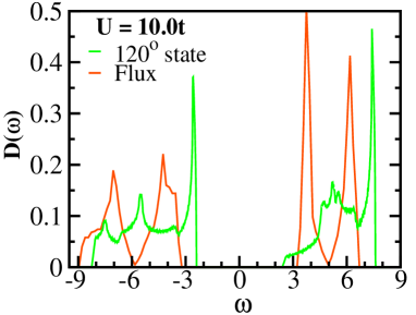
Figure 8: Color online: Electronic DOS in the ideal flux and $120$ degree spin configurations. For the same $U/t$ the $120$ degree state has a smaller gap than the flux phase.

We would like to point out the differences of our results in the present study, from the earlier studies [32] of the Mott transition on the checkerboard lattice. We address it in terms of the validity of our approximation in the $U-T$ plane based on $T=0$ and finite $T$ results. (i)At $T=0$, these three features are noteworthy. (a) The $U_{c}$ for the Mott transition: we obtain $U_{c}\sim 5.3t$, the only other value we know in the literature is $U_{c}\sim 6.7t$. These are in the same ballpark. (b) The large $U$ state: we obtain a flux like state while the stdudy [32] uses a more sophisticated approach to obtain a plaquette singlet state. Within our approach we believe the singlet state can be accessed only if we include quantum fluctuations of the ${\bf m}_{i}$’s. Both the plaquette singlet and the flux state lift the classical degeneracy of the Heisenberg limit but through different mechanisms. (c) The low $U$ metallic spin glass would be susceptible to quantum fluctuations, since it is a gapless state, and the Hartree-Fock result is likely to be modified in a full theory.
(ii)Finite $T$: While our $T=0$ results have the limitation of being Hartree-Fock, increasing $T$ brings into play the fluctuations that were suppressed at $T=0$. In fact as $T$ grows these classical fluctuations dominate over the quantum fluctuations and dictate the magnetic correlations and the electronic properties. To our knowledge, this aspect of checkerboard Mott physics has not been explored before.

4.2 Magnetic impact on electronic properties

Within our framework the electronic properties are dictated by the behaviour of the local moments, which in turn is decided by the electrons. We wish to establish a more quantitative connection between the magnetic order and the electronic DOS in some limiting cases.

For $T=0$ and $U\leq U_{c1}$ there are no local moments and the system is described by the tight-binding model. On the checkerboard structure this leads to a flat band at the upper band edge. For $U_{c1}\leq U<U_{c2}$ small moments show up, modifying the tight-binding DOS by broadening the flat band. For $U\geq U_{c2}$ the moments are sizable and they open a gap in the DOS. The ‘flux’ like order has a unique 4-peak structure in the DOS with a wide gap around the Fermi level. The $120$ degree ‘triangle’ phase shows pseudogap in the intermediate interaction window and has a gapped phase at strong interaction side. The specific behavior of the DOS in these magnetic ordered states can be understood as follows.

In the ‘flux’ phase, the local-moment at any lattice site ${\vec{R}}_{i}$ can be parametrized as $\vec{m_{i}}=(m_{ix},m_{iy},0)$ where

$$m_{ix} = \frac{m}{2}(e^{i\vec{Q_{F_{1}}}.\vec{R_{i}}}+e^{i\vec{Q_{F_{2}}}.\vec{R_{i}}})$$ (15)

$$m_{iy} = \frac{m}{2}(e^{i\vec{Q_{F_{2}}}.\vec{R_{i}}}-e^{i\vec{Q_{F_{1}}}.\vec{R_{i}}})$$

This magnetic ordering leads to two distinct energy levels at $\pm\frac{U}{2}$, each with a two-fold degeneracy. As electrons move on this magnetic background, they further split to bands $\pm(U/2)\pm t\sqrt{2+cos2k_{x}+cos2k_{y}}$. Thus the electron motion in the ‘flux’ phase gives rise to the unique 4-peak structure in the DOS. The minimum gap in the DOS for this state is $U-4t$.

In the ‘120 degree’ phase, the local-moment at any lattice site ${\vec{R}}_{i}$ can be parametrized as $\vec{m_{i}}=(m_{ix},m_{iy},0)$ where $m_{ix}=mcos({2\vec{Q_{T_{1}}}.\vec{R_{i}}})$,  $m_{iy}=msin({2\vec{Q_{T_{1}}}.\vec{R_{i}}})$. This phase also has two-fold degenerate energy levels at $\pm\frac{U}{2}$. Itinerant electrons on this magnetic background lift the degeneracy by $t[-g(k_{x},k_{y})\pm h(k_{x},k_{y})]/4$ where

$$g(k_{x},k_{y}) = [4cos(k_{x}-k_{y})+cos(k_{x}+k_{y})+\sqrt{3}sin(k_{x}+k_{y})]$$ (16)

$$h^{2}(k_{x},k_{y}) = [26+8cos(2k_{x}+2k_{y})-cos(2k_{x}-2k_{y})-8cos(2k_{x})$$

$$-8cos(2k_{y})-8cos(k_{x}+k_{y})+16cos(k_{x}-k_{y})$$

$$+\sqrt{3}sin(2k_{x}-2k_{y})-8\sqrt{3}sin(k_{x}+k_{y})-8\sqrt{3}sin(2k_{x})]$$

Thus the motion of electrons in the ‘120 degree’ phase retains the upper and lower Hubbard band features without undergoing any further splitting of bands (unlike the ‘flux’ phase). The minimum gap in the DOS for this state is $U-t[(h+g)_{max}+(h-g)_{max}]/4$. We observe that in the Brillouin zone $[(h+g)_{max}+(h-g)_{max}]>16$. Thus the gap for the ideal ‘flux’ phase is always larger than the ideal ‘120 degree’ phase for same interaction strength Fig.8.

5 CONCLUSION

We have studied the single band Hubbard model at half-filling on the checkerboard lattice. The Hartree-Fock ground state is non magnetic upto an interaction strength $U_{c1}$, then a small moment spin glass upto $U_{c2}$, and a ‘flux’ ordered state beyond. The Mott transition, associated with a gap opening in the density of states, occurs at $U_{c2}$. The presence of order differentiates this lattice of corner shared ‘tetrahedra’ from its three dimensional counterpart, the pyrochlore lattice, which remains disordered at all interaction strengths. A static auxiliary field based Monte Carlo provides an estimate of the temperature window over which the magnetic correlations survive. Strikingly, we observe that the flux order is replaced by a ‘120 degree’ correlated spin arrangement at intermediate temperature before all order is lost. We provide an entropic argument for this effect.

Acknowledgements: We acknowledge use of the HPC Clusters at HRI. NS appreciates discussing a variational calculation result with Ajanta Maity, and learning about a vector graphics language (Asymptote) from Rajarshi Tiwari. PM acknowledges support from an Outstanding Research Investigator Award of the Department of Atomic Energy-Science Research Council (DAE-SRC) of Government of India.

6 REFERENCES

References

- [1] Ramirez A P 1994 Annu. Rev. Mater. Sci. 24, 453.
- [2] Ong N P and Cava R J 2004 Science, 305, 52.
- [3] Balents L 2010 Nature, 464, 199.
- [4] Mott N F 1949 Proc. Roy. Soc. A 62, 416; Mott N F 1990 Metal-Insulator Transitions, Taylor and Francis.
- [5] Thouless D J 1965 Proc. Phys. Soc. 86, 893.
- [6] Roger M, Hetherington J H and Delrieu J M 1983 Rev. Mod. Phys. 55, 1.
- [7] Moessner R and Chalker J T 1998 Phys. Rev. B 58, 12049.
- [8] Limelette P, Wzietek P, Florens S, Georges A, Costi T A, Pasquier C, Jerome D, Meziere C and Batail P 2003 Phys. Rev. Lett., 91, 016401.
- [9] Parcollet O, Biroli G and Kotliar G 2004 Phys. Rev. Lett., 92, 226402.
- [10] Sahebsara P and Senechal D 2008 Phys. Rev. Lett., 100, 136402.
- [11] Clay R T, Li H and Mazumdar S 2008 Phys. Rev. Lett., 101, 166403.
- [12] Watanabe T, Yokoyama H, Tanaka Y and Inoue J 2008 Phys. Rev. B, 77, 214505.
- [13] Tiwari R and Majumdar P 2014 Europhys. Lett. 108, 27007.
- [14] Camjayi A, Acha C, Weht R, Rodriguez M G, Corraze B, Janod E, Cario L and Rozenberg M J 2014 Phys. Rev. Lett., 113, 086404.
- [15] Tiwari R and Majumdar P 2013 arXiv:1302.2922v1.
- [16] Timirgazin M A, Igoshev P A, Arzhnikov A K and Irkhin V Yu 2016 J. Phys.: Condens. Matter 28, 505601.
- [17] Ohashi T, Kawakami N and Tsunetsugu H 2006 Phys. Rev. Lett. 97, 066401.
- [18] Ohashi T, Momoi T, Tsunetsugu H and Kawakami N 2008 Prog. Ther. Phys. Suppl. 176, 97.
- [19] Fujimoto S 2001 Phys. Rev. B 64, 085102.
- [20] Swain N, Tiwari R and Majumdar P 2016 Phys. Rev. B 94, 155119.
- [21] Lieb E H and Schupp P 1999 Phys. Rev. Lett. 83, 5362.
- [22] Palmer S E and Chalker J T 2001 Phys. Rev. B 64, 94412.
- [23] Fouet J B, Mambrini M, Sindzingre P and Lhuillier C 2003 Phys. Rev. B 67, 54411.
- [24] Berg E, Altman E and Auerbach A 2003 Phys. Rev. Lett. 90, 147204.
- [25] Moessner R, Tchernyshyov O and Sondhi S 2004 Journal of Statistical Physics 116, 755.
- [26] Brenig W and Grzeschik M 2004 Phys. Rev. B 69(R), 064420.
- [27] Bernier J S, Chung C H, Kim Y B and Sachdev S 2004 Phys. Rev. B 69, 214427.
- [28] Shannon N, Misguich G and Penc K 2004 Phys. Rev. B 69, 220403.
- [29] Starykh O A, Furusaki A and Balents L 2005 Phys. Rev. B 72, 094416.
- [30] Nussinov Z, Batista C D, Normand B and Trugman S A 2007 Phys. Rev. B 75, 094411.
- [31] Fujimoto S 2003 Phys. Rev. B. 67, 235102.
- [32] Yoshioka T, Koga A and Kawakami N 2008 J. Phys. Soc. Jpn. 77, 104702.
- [33] Yokoyama H, Ogata M and Tanaka Y 2006 J. Phys. Soc. Jpn. 75, 114706.
- [34] Hubbard J 1979 Phys. Rev. B 19, 2626.
- [35] Stratonovich R L 1958 Sov. Phys. Doklady 2, 416; Hubbard J 1959 Phys. Rev. Lett. 3, 77.
- [36] Schulz H J 1990 Phys. Rev. Lett. 65, 2462.
- [37] Kumar S and Majumdar P 2006 Eur. Phys. J. B, 50, 571.
- [38] Binder K and Young A P 1986 Rev. Mod. Phys. 58, 801.
- [39] Villain J 1979 Z. Phys. B 33, 31.
- [40] Canals B 2002 Phys. Rev. B 65, 184408.
- [41] Tchernyshyov O, Starykh O A, Moessner R and Abanov A G 2003 Phys. Rev. B 68, 144422.
- [42] Hizi U and Henley C L 2006 Phys. Rev. B 73, 054403.