DESY 16-146 — KA-TP-24-2016 — ZU-TH 27/16
Distributions for neutral Higgs production in the

Abstract

A novel computation of the fully-differential cross section for neutral Higgs-boson production through gluon fusion in the $\mathcal{CP}$-conserving is presented. Based on the calculation of NLO corrections to the total cross section [1], we implemented the amplitudes in three codes, applying different resummation techniques: analytic transverse-momentum resummation at NLO+NLL, and two fully-differential NLO+PS Monte-Carlo approaches using the MC@NLO and POWHEG matching procedures, respectively. We study phenomenological predictions for distributions in the with a special emphasis on the Higgs transverse-momentum spectrum. Reasonable agreement among the various approaches is found, once well-motivated choices for the unphysical matching scales and the determination of the related uncertainties are made.

1 Introduction

The discovery of a scalar resonance in searches for a Higgs boson by the ATLAS [2] and CMS [3] collaborations is already considered as the legacy of Run I of the Large Hadron Collider (LHC). Although its measured properties are in full agreement with the Standard Model (SM) predictions so far, see e.g. Refs.[7, 8], the scalar particle may as well be embedded in an enlarged Higgs sector entailed in many beyond SM (BSM) theories. Among the most relevant of such SM extensions are supersymmetric models, with the Minimal Supersymmetric Standard Model (MSSM) being the simplest realization. The latter can be further extended to the Next-to-Minimal Supersymmetric Standard Model () by adding an SU$(2)_{L}$ singlet. This has the advantage of a dynamical generation of the $\mu$-term [9, 10], which lifts the upper bound on the mass of the lightest Higgs boson at tree level. Hence, a SM-like Higgs boson with a mass of $\sim 125$ GeV can be easily accommodated in the .

The $\mathcal{CP}$-conserving $\mathbb{Z}_{3}$-invariant entails five neutral Higgs bosons $\phi\in\{H_{1},H_{2},H_{3},A_{1},A_{2}\}$, three of which are $\mathcal{CP}$-even and two $\mathcal{CP}$-odd. While in the MSSM the light Higgs boson is identified with the observed SM-like Higgs resonance, the allows for phenomenologically interesting scenarios with lighter (pseudo-)scalar mass eigenstates. The direct search of further Higgs resonances is one of the central physics goals in LHC Run II. This requires precise theoretical predictions in explicit models for both inclusive and differential observables.

The most important Higgs-production mechanism in the SM is through gluon fusion. This remains true also in a large region of the parameter space of the (N)MSSM, which, in fact, favors lower values of $\tan\beta$ compared to the MSSM. In these cases the Higgs-gluon coupling is predominantly mediated by a top-quark loop. The total inclusive cross section has been computed in the limit of heavy top quarks at next-to-next-to-leading order (NNLO) [11, 12, 13] and recently at next-to-NNLO (N3LO) [14, 15]. Finite top-mass effects in the SM have been estimated to be below $1\%$ at NNLO [16, 17, 18, 19, 20, 21]. One must bear in mind, however, that in extended theories with two (or more) Higgs doublets the bottom-quark Yukawa coupling can be subject to a significantly enhancement, so that, on the one hand, the bottom-quark as a mediator of the Higgs-gluon coupling becomes equally or even more important than the top-quark. On the other hand, Higgs production in association with bottom quarks competes with the gluon-fusion process and can become the dominant production mode. The exact treatment of top and bottom-quark mass effects [32, 33] thus becomes vital for a precise prediction of Higgs cross sections in such theories. Squark and gluino effects at NLO QCD are known in certain approximations. Their expansion in heavy SUSY masses in the MSSM, see Refs.[34, 35, 36], was adapted to the in Ref.[1]. All these effects are implemented in the numerical code SusHi [37, 1, 38].

Kinematical distributions are an important tool in Higgs-boson measurements to distinguish the possible interplays between top- and bottom-quark, squark and gluino effects in the gluon-fusion scattering amplitude. This provides a precise discrimination between predictions in and beyond the SM, and allows for the determination of exclusion limits on the parameter space of BSM models. One of the most relevant differential observables in this respect is the Higgs transverse-momentum ($p_{T}$) spectrum. NLO [39, 40] and NNLO [41, 42, 43, 44, 45] QCD predictions for this observable are known only in the limit of heavy top quarks. Top-quark mass effects in the SM were found to be moderate ($\sim 2-3\%$) as long as momentum scales remain below roughly the top-quark mass or are integrated out [46, 47].

Predictions valid at all transverse momenta require small-$p_{T}$ resummation of logarithmically enhanced terms to all orders in the strong coupling constant ($\alpha_{s}$). Such resummation can be derived from universal properties of QCD radiation in the infra-red region [48, 49, 50, 51, 52, 53, 54, 55, 56, 57], and can be performed analytically or by means of a numerical parton shower (PS) approach. In the MSSM, the analytically resummed Higgs transverse-momentum spectrum in gluon fusion has been computed at next-to-leading logarithmic (NLL) accuracy with a consistent matching to the NLO fixed-order cross section [63, 64], while fully-differential NLO predictions matched to parton showers (NLO+PS) were first presented in the POWHEG approach [65, 66] in Ref.[67], and later in a MC@NLO-type matching [68] in Ref.[69].

Common to all three approaches (analytic resummation, MC@NLO, POWHEG) is an effective matching scale (resummation scale, shower scale, $h_{\rm fact}$) that controls the separation between the soft/collinear and the hard region. Although the dependence on the matching scales is of higher logarithmic order, suitable choices turn out to be absolutely crucial in particular when the bottom loop is involved. We refer the reader to Refs.[64, 70], where two proposals for their algorithmic determination are made, and to Ref.[71] for the comprehensive comparison of these proposals.

In this letter, we present a novel computation of differential Higgs-boson production through gluon fusion in the and report on new implementations of effects in three different codes, which all apply the SusHi amplitudes for the computation of the matrix elements:

• MoRe-SusHi [63, 64, 72] performs analytic transverse-momentum resummation at NLO+NLL.

• aMCSusHi [69, 73] employs the MadGraph5_aMC@NLO framework [74] to compute NLO+PS predictions with the MC@NLO method.

• POWHEG-SusHi [76] uses the corresponding POWHEG implementation for the NLO+PS matching in the POWHEG BOX framework [77].

2 The Higgs sector of the

We start with a discussion of the Higgs sector of the $\mathcal{CP}$-conserving $\mathbb{Z}_{3}$-invariant , which closely follows Refs.[78, 1]. If we denote the superpotential of the MSSM (without $\mu$-term) by $W_{\rm{MSSM}}$, the one of the is given by

$$W_{\rm\nmssm}=W_{\rm{MSSM}}-\epsilon_{ab}\lambda\hat{S}\hat{H}_{d}^{a}\hat{H}_{u}^{b}+\frac{1}{3}\kappa\hat{S}^{3}\,,$$ (1)

where $\hat{H}_{d}$ and $\hat{H}_{u}$ are the two SU$(2)_{L}$ doublet superfields known from the MSSM and $\hat{S}$ is the additional SU$(2)_{L}$ singlet superfield. The tensor $\epsilon_{ab}$ contracts the components of the SU$(2)_{L}$ doublets. The singlet $\hat{S}$ is a neutral superfield and thus the contains one additional $\mathcal{CP}$-even and $\mathcal{CP}$-odd (two and three in total) neutral Higgs boson compared to the MSSM. The soft-breaking terms can be written in the form

$$\mathcal{L}_{\text{soft}}=\mathcal{L}_{\text{soft},{MSSM}}+(\epsilon_{ab}\lambda A_{\lambda}SH_{d}^{a}H_{u}^{b}-\frac{1}{3}\kappa A_{\kappa}S^{3}+\text{h.c.})-m_{s}^{2}|S|^{2}\,.$$ (2)

Similar to $m_{H_{d}}^{2}$ and $m_{H_{u}}^{2}$ in the MSSM, the mass term $m_{s}^{2}$ can be obtained from the minimization conditions of the tadpole equations. We consider $A_{\lambda}$ and $A_{\kappa}$ as input parameters. Alternatively, $A_{\lambda}$ can be replaced by the mass $m_{H^{\pm}}$ of the charged Higgs boson as input parameter. We decompose the neutral components of the Higgs fields as follows

$$H_{u}^{0}=\frac{1}{\sqrt{2}}(v_{u}+H_{u}^{R}+iH_{u}^{I})\,,\quad H_{d}^{0}=\frac{1}{\sqrt{2}}(v_{d}+H_{d}^{R}+iH_{d}^{I})\,,\quad S=\frac{1}{\sqrt{2}}(v_{s}+S^{R}+iS^{I})\,,$$ (3)

where $v_{d},v_{u}$ and $v_{s}$ are the vacuum expectation values (VEVs) and the fields with indices $R$ and $I$ denote the $\mathcal{CP}$-even and -odd fluctuations around the VEVs. The VEV of the singlet is $v_{s}$ and generates an effective $\mu$-term $\mu_{\rm eff}=\lambda v_{s}/\sqrt{2}$, which is considered also as input parameter. Consequently $v_{s}$ is determined by $\lambda$ and $\mu_{\rm eff}$. We refrain from a detailed discussion of the mass matrices, but rather refer to Ref.[78]. The mixing matrices, transforming the gauge into mass eigenstates, are crucial though. For this purpose we define the basis of $\mathcal{CP}$-even gauge eigenstates $H^{R}=(H_{d}^{R},H_{u}^{R},S^{R})$ and the one of the $\mathcal{CP}$-odd eigenstates $H^{I}=(H_{d}^{I},H_{u}^{I},S^{I}$). In this notation the mass eigenstates $H_{i}$ with $i\in\{1,2,3\}$ in the $\mathcal{CP}$-even case are easily obtained through a single rotation with a $(3\times 3)$-matrix

$$H_{i}=\sum_{j=1}^{3}\mathcal{R}^{S}_{ij}H^{R}_{j}\,.$$ (4)

In the $\mathcal{CP}$-odd sector we perform a prerotation $\mathcal{R}^{G}$ such that the intermediate basis is given by $H^{\prime I}=(A,S^{I},G)$ with the Goldstone boson as last entry. The final mass eigenstates $A_{i}$ with $i\in\{1,2\}$ are obtained through

$$A_{i}=\sum_{j=1}^{3}\mathcal{R}^{P}_{ij}H^{\prime I}_{j}=\sum_{j,k=1}^{3}\mathcal{R}^{P}_{ij}\mathcal{R}^{G}_{jk}H^{I}_{k}\quad\text{with}\quad\mathcal{R}^{G}=\begin{pmatrix}s_{\beta}&c_{\beta}&0\\ 0&0&1\\ c_{\beta}&-s_{\beta}&0\end{pmatrix}\,.$$ (5)

The $(3\times 3)$-matrix $\mathcal{R}^{P}$ consists of a $(2\times 2)$-mixing block, whereas $\mathcal{R}^{P}_{i3}=\mathcal{R}^{P}_{3i}=0$ for $i\neq 3$ and $\mathcal{R}^{P}_{33}=1$. The mass spectrum and Higgs mixing matrices can thus be easily taken over from various spectrum generators, see Ref.[79] and references therein.

For the subsequent study we pick a benchmark scenario (named BP2_P2) provided by the LHC Higgs Cross Section Working Group [80], which is based on Refs.[81, 82] and defined by

$$\tan\beta=2.266,\;\lambda=0.644,\;\kappa=0.351,\;\mu_{\rm eff}=178~{}\text{GeV},\;A_{\kappa}=100~{}\text{GeV},\;A_{\lambda}=-312~{}\text{GeV}\,.$$ (6)

We use NMSSMTools 4.7.0 [83, 84, 85, 86] to obtain the Higgs spectrum with masses

$$\begin{split}&m_{H_{1}}=125.9~{}\text{GeV},\quad m_{H_{2}}=201.0~{}\text{GeV},\quad m_{H_{3}}=448.1~{}\text{GeV}\\ &m_{A_{1}}=65.2~{}\text{GeV},\quad m_{A_{2}}=440.0~{}\text{GeV}\,.\end{split}$$ (7)

The input parameters of the relevant colored SUSY particles are given by

$$\begin{split}&m_{\tilde{g}}=2222~{}\text{GeV},\quad A_{t}=-1630~{}\text{GeV},\quad A_{b}=-3376~{}\text{GeV},\\ &m_{Q}=1710~{}\text{GeV},\quad m_{U}=1046~{}\text{GeV},\quad m_{D}=2064~{}\text{GeV}\,,\end{split}$$ (8)

where $m_{Q},m_{U},m_{D},A_{t}$ and $A_{b}$ are the soft-breaking parameters of the third-generation squark sector in $\mathcal{L}_{\text{soft},{MSSM}}$ of Eq. (2). The light scalar in that scenario is SM-like and thus consistent with data of LHC Run I. Furthermore, the low-mass pseudo-scalar is compatible with LHC and LEP searches. We note that the scenario features heavy squarks and gluinos, with on-shell masses above $1$ TeV, lowering their impact on the gluon-fusion cross section.

We subsequently discuss differential results for the two singlet-like Higgs bosons $A_{1}$ and $H_{2}$ as well as one standard heavy Higgs boson $H_{3}$. By contrast, we refrain from discussing the SM-like Higgs boson $H_{1}$ as well as the MSSM-like pseudoscalar $A_{2}$ as they do not provide new features.

We also do not consider a benchmark scenario with a singlet-like (pseudo-)scalar, for which quark-contributions tend to cancel each other and squark as well as electro-weak contributions are accordingly large, see Ref.[1] for an example, since the cross section in such a case is rather small and the experimental determination of the transverse-momentum spectrum remains very challenging even in LHC Run II.

3 Differential cross sections in the

(a)		(b)		(c)		(d)
(e)		(f)		(g)		(h)

Figure 1: A sample of Feynman diagrams for $gg\rightarrow\phi$ contributing to the NLO cross section; (a-c) LO, (d-f) virtual and (g-h) real corrections. The graphical notation for the lines is: solid straight $\widehat{=}$ quark; spiraled $\widehat{=}$ gluon; dashed $\widehat{=}$ scalar (squark or Higgs); spiraled with line $\widehat{=}$ gluino.

The generic leading-order diagrams for Higgs production in the , i.e., $gg\rightarrow\phi$ with $\phi\in\{H_{1},H_{2},H_{3},A_{1},A_{2}\}$, are induced by a quark or squark loop, as shown in Fig. 1 (a-c). At NLO each of these diagrams receives virtual corrections by a gluon or gluino exchange, e.g., Fig. 1 (d-e), or by an additional squark loop, e.g., Fig. 1 (f). Additionally, real emission contributions must be included, which involve also diagrams with further initial-state partons, see Fig. 1 (g-h) for example. The corresponding matrix elements are implemented in and taken from the code SusHi [1, 37, 38].

They are combined and matched to all-order results in three different resummation frameworks. The analytic resummation of soft and collinear logarithms as formulated in Ref.[56] with the matching procedure developed in Ref.[87] allows for the prediction of a single differential observable, the inclusive transverse-momentum spectrum of the Higgs boson, but with the highest possible order in the logarithmic series, i.e., NLL accuracy in the (N)MSSM. Monte-Carlo approaches perform resummation numerically by means of a parton shower. The matching to the NLO cross section is done by the well-known MC@NLO [68] and POWHEG [65, 66] methods. They allow for the computation of arbitrary infra-red safe observables at NLO+PS, but consistently resum only the leading logarithms and partially the ones beyond. For the Monte-Carlo simulations we use the framework of MadGraph5_aMC@NLO and POWHEG BOX, respectively, which support all standard parton showers [88, 89, 90, 91, 92, 93].

All phenomenological results in this letter are obtained with the codes MoRe-SusHi, aMCSusHi and POWHEG-SusHi. In particular, we employ the modified POWHEG (mPOWHEG) matching to the shower as suggested in Ref.[71] for all the POWHEG-SusHi results, by restricting the shower starting scale to a fixed value instead of using the transverse momentum of the first emission, which may become arbitrarily large. This has the advantage of limiting the impact of the parton shower at large transverse momenta, where it is outside its validity region and the fixed-order result gives a viable prediction, and warrants a smooth merging of the matched result into the fixed-order cross section at large transverse momenta.

We work at the $13$ TeV LHC and use the MSTW2008 $68$%CL NLO PDF sets [94], with the associated value of the strong coupling constant. Top and bottom-quark masses are renormalized on-shell both in the matrix elements and for the Yukawa couplings, and set to the pole masses $m_{t}=172.5$ GeV and $m_{b}=4.75$ GeV, respectively. We use dynamical central renormalization and factorization scales of $\mu_{\rm R}=\mu_{\rm F}=H_{T}/2\equiv 1/2\,\sum_{i}(m_{i}^{2}+p_{T}^{2}(i))^{1/2}$ ($i$ runs over all final-state particles, with $m_{i}$ and $p_{T}(i)$ being their respective mass and transverse momentum) for the Monte-Carlo predictions and $\mu_{\rm R}=\mu_{\rm F}=m_{T}/2\equiv 1/2\,(m_{\phi}^{2}+p_{T}^{2}(\phi))^{1/2}$ in analytic resummation and the fixed order distribution (fNLO). The matching scales in the various approaches (resummation scale, shower scale, $h_{\rm fact}$) are chosen as suggested in Ref.[64, 71], see also Ref.[69] regarding the implications for the dynamical shower scale choice in aMCSusHi. As far as the Monte-Carlo approaches are concerned, we use the Pythia8 [91] parton shower.

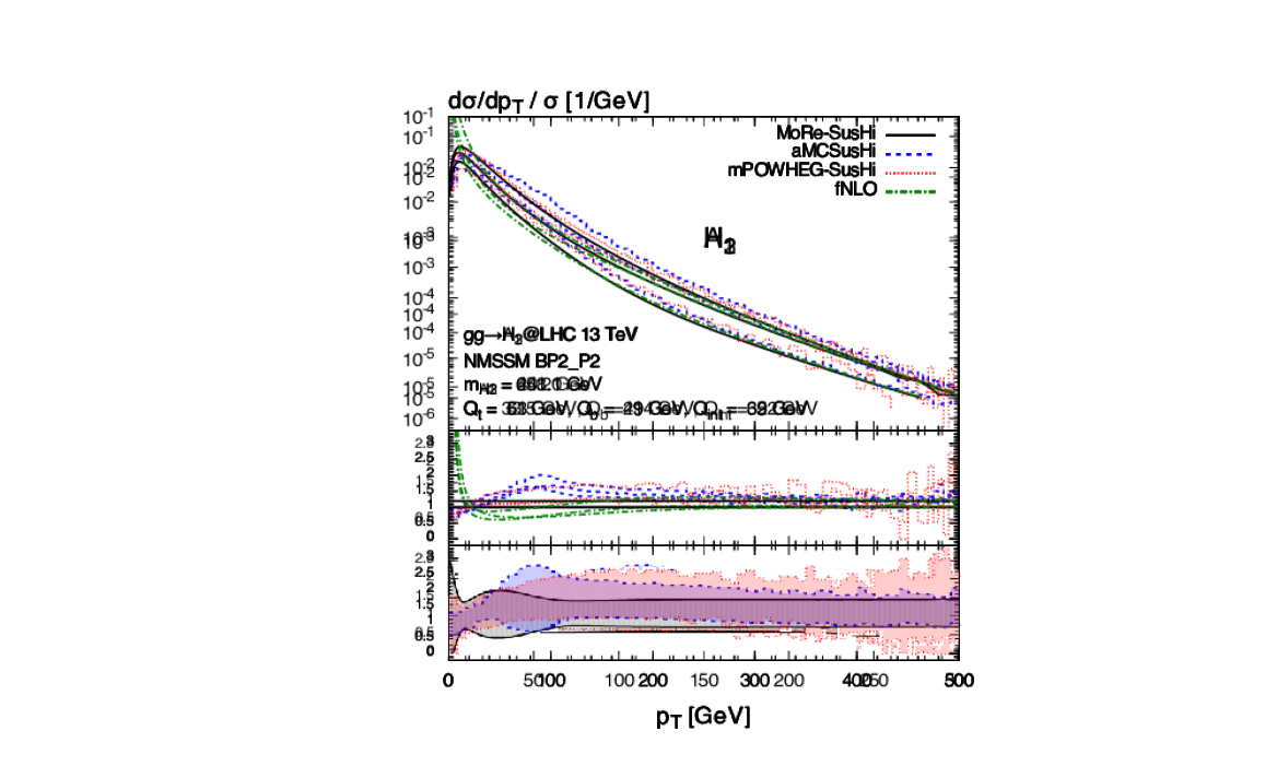
 (a)

 (b)

Figure 2: Transverse-momentum distributions of the two heavy scalars of the scenario introduced in Section 2; (a) $H_{2}$; and (b) $H_{3}$. See text for the description of the different curves.

In Fig. 2 we compare the predictions for the inclusive transverse-momentum distributions of the heavy scalar Higgs bosons in the benchmark scenario BP2_P2 (see Section 2) among the various approximations: NLO+NLL analytic resummation (black, solid), NLO+PS in the MC@NLO (blue, dashed), and the mPOWHEG (red, dotted) and, for reference, fNLO (green, dash-dotted) which formally corresponds to LO as far as the $p_{T}$ distribution is concerned. The fNLO curve is computed with the same central scales as the analytically resummed result; we checked, however, that there are only minor differences to the scale adopted in the two Monte Carlos and only at very large $p_{T}$. The bands correspond to a 7-point $(\mu_{\rm R}{}$, $\mu_{\rm F}{})$ variation by a factor of two around the central scale. The variation of the matching scale in each approach is done also by a factor of two and added in quadrature. In the case of analytic resummation, we apply, however, a suppression factor to the resummation-scale dependence, as introduced in Ref.[64], at large transverse momenta, since any dependence of the cross section on its value is necessarily artificial in the large-$p_{T}$ region.

The left and right panels of Fig. 2 correspond to the results for $H_{2}$ with $m_{H_{2}}=201.0$ GeV and $H_{3}$ with $m_{H_{3}}=448.1$ GeV, respectively. The features of the two plots are fairly similar, which allows us to discuss them simultaneously. The general observations are the following:

• Overall, the agreement among the different codes is reasonably well within the respective uncertainties, which are generally large though, in particular at high transverse momenta.

• The analytically resummed curve of MoRe-SusHi is softer than the Monte-Carlo results. The two Monte-Carlo results are hardly distinguishable at very small transverse momenta ($0$ GeV$\leq p_{T}\leq 40$ GeV), which is driven by the underlying Pythia8 shower. Also, the difference to MoRe-SusHi in that region is not very big either, reaching up to $\mathcal{O}(30$-$40\%)$ only in the first bin.

• In the intermediate-$p_{T}$ region ($50$ GeV$\lesssim p_{T}\lesssim 250$ GeV) the MC@NLO prediction of aMCSusHi develops a somewhat larger uncertainty band than the other two approaches. As shown in Ref.[71] the main reason for this is the dynamical shower scale adopted from MadGraph5_aMC@NLO. Within that region (around $p_{T}{}\sim 100$ GeV) also the central aMCSusHi prediction deviates from the other results by $\mathcal{O}(50\%)$, which in turn are in rather well agreement, in particular regarding their shapes.

• At large transverse momenta ($p_{T}\geq 250$ GeV), both Monte-Carlo predictions feature uncertainties that are larger than the ones of MoRe-SusHi, the POWHEG band being particularly sizable in that region. One should bear in mind, however, that for MoRe-SusHi we turned off uncertainties related to the resummation scale in that $p_{T}$ region. We further note that by construction both MC@NLO and mPOWHEG results will eventually merge into the fixed-order result at sufficiently large transverse momenta also with respect to the scale uncertainties. Indeed, we already see the smooth matching to the fixed-order curve at large $p_{T}$ for the central curves. Though small differences will remain due to the slightly different choices adopted for the central scales of fNLO and the two Monte Carlos.

• We finally remark that the general differences we observe among the codes are very reminiscent to what has been found in Ref.[71] in case of generic 2HDM Higgs bosons. The general conclusions drawn in that paper are thus also applicable to the , since the paper captures different hierarchies between top- and bottom-Yukawa couplings.

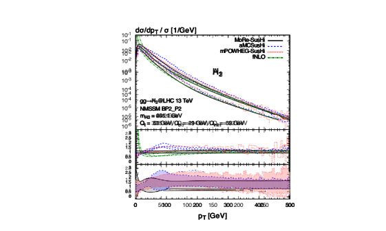
Figure 3: Same as Fig. 2, but for the light pseudo-scalar Higgs boson $A_{1}$.

We now turn to the transverse-momentum distribution of the light pseudo-scalar Higgs boson ($A_{1}$) with $m_{A_{1}}=65.2$ GeV, shown in Fig. 3. The general features are not very different as compared to the heavy scalars in Fig. 2. Most remarkable, however, is the excellent agreement between the central predictions of the two Monte Codes in this case, except for the small bump of the aMCSusHi curve around $p_{T}\sim 40-70$ GeV. Similar to the scalar Higgs case also for the light pseudo-scalar particle the uncertainty in the MC@NLO matching blows up, although to a lesser extend, and the POWHEG curve develops a wider uncertainty band in the high-$p_{T}$ region. The analytically resummed result of MoRe-SusHi again shows a generally softer spectrum, most apparent at small transverse momenta, while the uncertainties in that region are quite similar to the ones of the Monte Carlos, with a somewhat larger band though as $p_{T}\rightarrow 0$. The smaller band of MoRe-SusHi at high $p_{T}$ is again caused by the suppression of the resummation-scale variations, although one already observes also for the aMCSusHi prediction the smooth merging into the fixed-order result. Overall, the agreement of the various predictions is well within their respective uncertainties. We finally note that care must be taken, when considering very low Higgs boson masses ($m_{\phi}\lesssim 20$ GeV) in computations such as the one at hand, since the Higgs mass approaches quark thresholds, e.g. $2m_{b}$, which requires the resummation of gluon effects.

4 Conclusions

We have presented predictions for Higgs-boson production through gluon fusion in the . For the first time tools are made available to simulate a Higgs signal at NLO QCD accuracy matched to parton showers and to compute the Higgs transverse-momentum distribution analytically at NLO+NLL. We have considered the transverse-momentum distribution of various Higgs bosons in a benchmark scenario, including the phenomenologically interesting case of a light pseudo-scalar of mass well below the observed scalar resonance. The comparison of the predictions obtained with the three codes turned out to show rather similar features as the ones already observed in the MSSM. Overall, the agreement among these predictions is well within the theoretical uncertainty bands. Each of these codes, therefore, provides a proper modelling of the Higgs transverse-momentum spectrum, as long as the relevant (perturbative and resummation-related) scale uncertainties are kept into account.

The computations presented in this letter enable a reliable simulation of a Higgs signal within the and will serve particularly useful in this respect to light and heavy Higgs-boson searches by the experiments at the LHC. The combination of the gluon-induced cross-section predictions with the ones obtained for Higgs-boson production in association with bottom quarks, which becomes relevant in scenarios with an enhanced bottom-quark Yukawa coupling, was not discussed in this letter. However, Higgs-boson production in association with bottom quarks and its distributions can be reweighted from the corresponding SM results and incoherently added to the gluon-fusion cross section. Finally, off-shell effects become relevant for Higgs-boson masses around (and above) the TeV scale; their inclusion in the codes at hand is feasible, but beyond the scope of this letter.

Acknowledgements.

We would like to thank the LHC Higgs Cross Section Working Group for providing the motivation to perform this computation. This research was supported in part by the Swiss National Science Foundation (SNF) under contract 200021-156585 and by Deutsche Forschungsgemeinschaft through the SFB 676 “Particles, Strings, and the Early Universe”.

References

- [1] S. Liebler, Eur. Phys. J. C75, 210 (2015), arXiv:1502.07972.
- [2] ATLAS, G. Aad et al., Phys. Lett. B716, 1 (2012), arXiv:1207.7214.
- [3] CMS, S. Chatrchyan et al., Phys. Lett. B716, 30 (2012), arXiv:1207.7235.
- [4] LHC Higgs Cross Section Working Group, S. Dittmaier et al., (2011), arXiv:1101.0593.
- [5] LHC Higgs Cross Section Working Group, S. Dittmaier et al., (2012), arXiv:1201.3084.
- [6] LHC Higgs Cross Section Working Group, J. R. Andersen et al., (2013), arXiv:1307.1347.
- [7] ATLAS, G. Aad et al., Eur. Phys. J. C75, 476 (2015), arXiv:1506.05669.
- [8] CMS, V. Khachatryan et al., Eur. Phys. J. C75, 212 (2015), arXiv:1412.8662.
- [9] U. Ellwanger, C. Hugonie, and A. M. Teixeira, Phys. Rept. 496, 1 (2010), arXiv:0910.1785.
- [10] M. Maniatis, Int. J. Mod. Phys. A25, 3505 (2010), arXiv:0906.0777.
- [11] R. V. Harlander and W. B. Kilgore, Phys. Rev. Lett. 88, 201801 (2002), arXiv:hep-ph/0201206.
- [12] C. Anastasiou and K. Melnikov, Nucl. Phys. B646, 220 (2002), arXiv:hep-ph/0207004.
- [13] V. Ravindran, J. Smith, and W. L. van Neerven, Nucl. Phys. B665, 325 (2003), arXiv:hep-ph/0302135.
- [14] C. Anastasiou, C. Duhr, F. Dulat, F. Herzog, and B. Mistlberger, Phys. Rev. Lett. 114, 212001 (2015), arXiv:1503.06056.
- [15] C. Anastasiou et al., JHEP 05, 058 (2016), arXiv:1602.00695.
- [16] S. Marzani, R. D. Ball, V. Del Duca, S. Forte, and A. Vicini, Nucl. Phys. B800, 127 (2008), arXiv:0801.2544.
- [17] R. V. Harlander and K. J. Ozeren, Phys. Lett. B679, 467 (2009), arXiv:0907.2997.
- [18] R. V. Harlander and K. J. Ozeren, JHEP 11, 088 (2009), arXiv:0909.3420.
- [19] R. V. Harlander, H. Mantler, S. Marzani, and K. J. Ozeren, Eur. Phys. J. C66, 359 (2010), arXiv:0912.2104.
- [20] A. Pak, M. Rogal, and M. Steinhauser, JHEP 02, 025 (2010), arXiv:0911.4662.
- [21] A. Pak, M. Rogal, and M. Steinhauser, JHEP 09, 088 (2011), arXiv:1107.3391.
- [22] E. Bagnaschi et al., JHEP 06, 167 (2014), arXiv:1404.0327.
- [23] J. M. Campbell, R. K. Ellis, F. Maltoni, and S. Willenbrock, Phys. Rev. D67, 095002 (2003), arXiv:hep-ph/0204093.
- [24] R. V. Harlander and W. B. Kilgore, Phys. Rev. D68, 013001 (2003), arXiv:hep-ph/0304035.
- [25] S. Dittmaier, M. Krämer, and M. Spira, Phys. Rev. D70, 074010 (2004), arXiv:hep-ph/0309204.
- [26] S. Dawson, C. B. Jackson, L. Reina, and D. Wackeroth, Phys. Rev. D69, 074027 (2004), arXiv:hep-ph/0311067.
- [27] R. V. Harlander, K. J. Ozeren, and M. Wiesemann, Phys. Lett. B693, 269 (2010), arXiv:1007.5411.
- [28] R. V. Harlander and M. Wiesemann, JHEP 04, 066 (2012), arXiv:1111.2182.
- [29] S. Bühler, F. Herzog, A. Lazopoulos, and R. Müller, JHEP 07, 115 (2012), arXiv:1204.4415.
- [30] R. V. Harlander, A. Tripathi, and M. Wiesemann, Phys. Rev. D90, 015017 (2014), arXiv:1403.7196.
- [31] M. Wiesemann et al., JHEP 02, 132 (2015), arXiv:1409.5301.
- [32] M. Spira, A. Djouadi, D. Graudenz, and P. M. Zerwas, Nucl. Phys. B453, 17 (1995), arXiv:hep-ph/9504378.
- [33] R. V. Harlander and P. Kant, JHEP 12, 015 (2005), arXiv:hep-ph/0509189.
- [34] G. Degrassi and P. Slavich, JHEP 11, 044 (2010), arXiv:1007.3465.
- [35] G. Degrassi, S. Di Vita, and P. Slavich, JHEP 08, 128 (2011), arXiv:1107.0914.
- [36] G. Degrassi, S. Di Vita, and P. Slavich, Eur. Phys. J. C72, 2032 (2012), arXiv:1204.1016.
- [37] R. V. Harlander, S. Liebler, and H. Mantler, Comput. Phys. Commun. 184, 1605 (2013), arXiv:1212.3249.
- [38] R. V. Harlander, S. Liebler, and H. Mantler, (2016), arXiv:1605.03190.
- [39] D. de Florian, M. Grazzini, and Z. Kunszt, Phys. Rev. Lett. 82, 5209 (1999), arXiv:hep-ph/9902483.
- [40] C. J. Glosser and C. R. Schmidt, JHEP 12, 016 (2002), arXiv:hep-ph/0209248.
- [41] R. Boughezal, F. Caola, K. Melnikov, F. Petriello, and M. Schulze, JHEP 06, 072 (2013), arXiv:1302.6216.
- [42] X. Chen, T. Gehrmann, E. W. N. Glover, and M. Jaquier, Phys. Lett. B740, 147 (2015), arXiv:1408.5325.
- [43] R. Boughezal, F. Caola, K. Melnikov, F. Petriello, and M. Schulze, Phys. Rev. Lett. 115, 082003 (2015), arXiv:1504.07922.
- [44] R. Boughezal, C. Focke, W. Giele, X. Liu, and F. Petriello, Phys. Lett. B748, 5 (2015), arXiv:1505.03893.
- [45] F. Caola, K. Melnikov, and M. Schulze, Phys. Rev. D92, 074032 (2015), arXiv:1508.02684.
- [46] R. V. Harlander, T. Neumann, K. J. Ozeren, and M. Wiesemann, JHEP 08, 139 (2012), arXiv:1206.0157.
- [47] T. Neumann and M. Wiesemann, JHEP 11, 150 (2014), arXiv:1408.6836.
- [48] Y. L. Dokshitzer, D. Diakonov, and S. I. Troian, Phys. Rept. 58, 269 (1980).
- [49] G. Parisi and R. Petronzio, Nucl. Phys. B154, 427 (1979).
- [50] G. Curci, M. Greco, and Y. Srivastava, Nucl. Phys. B159, 451 (1979).
- [51] J. C. Collins and D. E. Soper, Nucl. Phys. B193, 381 (1981), [Erratum: Nucl. Phys.B213,545(1983)].
- [52] J. C. Collins and D. E. Soper, Nucl. Phys. B197, 446 (1982).
- [53] J. Kodaira and L. Trentadue, Phys. Lett. B112, 66 (1982).
- [54] J. Kodaira and L. Trentadue, Phys. Lett. B123, 335 (1983).
- [55] G. Altarelli, R. K. Ellis, M. Greco, and G. Martinelli, Nucl. Phys. B246, 12 (1984).
- [56] J. C. Collins, D. E. Soper, and G. F. Sterman, Nucl. Phys. B250, 199 (1985).
- [57] S. Catani, D. de Florian, and M. Grazzini, Nucl. Phys. B596, 299 (2001), arXiv:hep-ph/0008184.
- [58] C. W. Bauer, S. Fleming, and M. E. Luke, Phys. Rev. D63, 014006 (2000), arXiv:hep-ph/0005275.
- [59] C. W. Bauer, S. Fleming, D. Pirjol, and I. W. Stewart, Phys. Rev. D63, 114020 (2001), arXiv:hep-ph/0011336.
- [60] C. W. Bauer and I. W. Stewart, Phys. Lett. B516, 134 (2001), arXiv:hep-ph/0107001.
- [61] C. W. Bauer, D. Pirjol, and I. W. Stewart, Phys. Rev. D65, 054022 (2002), arXiv:hep-ph/0109045.
- [62] M. Beneke, A. P. Chapovsky, M. Diehl, and T. Feldmann, Nucl. Phys. B643, 431 (2002), arXiv:hep-ph/0206152.
- [63] H. Mantler and M. Wiesemann, Eur. Phys. J. C73, 2467 (2013), arXiv:1210.8263.
- [64] R. V. Harlander, H. Mantler, and M. Wiesemann, JHEP 11, 116 (2014), arXiv:1409.0531.
- [65] P. Nason, JHEP 11, 040 (2004), arXiv:hep-ph/0409146.
- [66] S. Frixione, P. Nason, and C. Oleari, JHEP 11, 070 (2007), arXiv:0709.2092.
- [67] E. Bagnaschi, G. Degrassi, P. Slavich, and A. Vicini, JHEP 02, 088 (2012), arXiv:1111.2854.
- [68] S. Frixione and B. R. Webber, JHEP 06, 029 (2002), arXiv:hep-ph/0204244.
- [69] H. Mantler and M. Wiesemann, Eur. Phys. J. C75, 257 (2015), arXiv:1504.06625.
- [70] E. Bagnaschi and A. Vicini, JHEP 01, 056 (2016), arXiv:1505.00735.
- [71] E. Bagnaschi, R. V. Harlander, H. Mantler, A. Vicini, and M. Wiesemann, JHEP 01, 090 (2016), arXiv:1510.08850.
- [72] http://sushi.hepforge.org/moresushi.html .
- [73] https://cp3.irmp.ucl.ac.be/projects/madgraph/wiki/aMCSushi .
- [74] J. Alwall et al., JHEP 07, 079 (2014), arXiv:1405.0301.
- [75] R. Frederix, S. Frixione, E. Vryonidou, and M. Wiesemann, JHEP 08, 006 (2016), arXiv:1604.03017.
- [76] H. Mantler, to appear .
- [77] S. Alioli, P. Nason, C. Oleari, and E. Re, JHEP 06, 043 (2010), arXiv:1002.2581.
- [78] K. Ender, T. Graf, M. Mühlleitner, and H. Rzehak, Phys. Rev. D85, 075024 (2012), arXiv:1111.4952.
- [79] F. Staub et al., Comput. Phys. Commun. 202, 113 (2016), arXiv:1507.05093.
- [80] https://twiki.cern.ch/twiki/bin/view/LHCPhysics/LHCHXSWGNMSSM#BP2 .
- [81] N.-E. Bomark, S. Moretti, S. Munir, and L. Roszkowski, JHEP 02, 044 (2015), arXiv:1409.8393.
- [82] N.-E. Bomark, S. Moretti, and L. Roszkowski, (2015), arXiv:1503.04228.
- [83] U. Ellwanger, J. F. Gunion, and C. Hugonie, JHEP 02, 066 (2005), arXiv:hep-ph/0406215.
- [84] U. Ellwanger and C. Hugonie, Comput. Phys. Commun. 175, 290 (2006), arXiv:hep-ph/0508022.
- [85] G. Belanger, F. Boudjema, C. Hugonie, A. Pukhov, and A. Semenov, JCAP 0509, 001 (2005), arXiv:hep-ph/0505142.
- [86] U. Ellwanger and C. Hugonie, Comput. Phys. Commun. 177, 399 (2007), arXiv:hep-ph/0612134.
- [87] G. Bozzi, S. Catani, D. de Florian, and M. Grazzini, Nucl. Phys. B737, 73 (2006), arXiv:hep-ph/0508068.
- [88] G. Corcella et al., JHEP 01, 010 (2001), arXiv:hep-ph/0011363.
- [89] G. Corcella et al., (2002), arXiv:hep-ph/0210213.
- [90] T. Sjöstrand, S. Mrenna, and P. Z. Skands, JHEP 05, 026 (2006), arXiv:hep-ph/0603175.
- [91] T. Sjöstrand, S. Mrenna, and P. Z. Skands, Comput. Phys. Commun. 178, 852 (2008), arXiv:0710.3820.
- [92] M. Bahr et al., Eur. Phys. J. C58, 639 (2008), arXiv:0803.0883.
- [93] J. Bellm et al., (2013), arXiv:1310.6877.
- [94] A. D. Martin, W. J. Stirling, R. S. Thorne, and G. Watt, Eur. Phys. J. C63, 189 (2009), arXiv:0901.0002.
- [95] A. Buckley et al., Eur. Phys. J. C75, 132 (2015), arXiv:1412.7420.