To appear in The Astrophysical Journal
Graphite Revisited

Abstract

Laboratory measurements are used to constrain the dielectric tensor for graphite, from microwave to X-ray frequencies. The dielectric tensor is strongly anisotropic even at X-ray energies. The discrete dipole approximation is employed for accurate calculations of absorption and scattering by single-crystal graphite spheres and spheroids. For randomly-oriented single-crystal grains, the so-called $\nicefrac{{1}}{{3}}$ - $\nicefrac{{2}}{{3}}$ approximation for calculating absorption and scattering cross sections is exact in the limit $a/\lambda\rightarrow 0$, provides better than $\sim$10% accuracy in the optical and UV even when $a/\lambda$ is not small, but becomes increasingly inaccurate at infrared wavelengths, with errors as large as $\sim$40% at $\lambda=10\micron$. For turbostratic graphite grains, the Bruggeman and Maxwell Garnett treatments yield similar cross sections in the optical and ultraviolet, but diverge in the infrared, with predicted cross sections differing by over an order of magnitude in the far-infrared. It is argued that the Maxwell Garnett estimate is likely to be more realistic, and is recommended. The out-of-plane lattice resonance of graphite near $11.5\micron$ may be observable in absorption with the MIRI spectrograph on JWST. Aligned graphite grains, if present in the ISM, could produce polarized X-ray absorption and polarized X-ray scattering near the carbon K edge.

1 Introduction

First proposed as an interstellar grain material by Cayrel & Schatzman (1954) and Hoyle & Wickramasinghe (1962), the graphite hypothesis received support with the discovery by Stecher (1965) of a strong extinction “bump” at $2175\,{\rm\AA}$, consistent with the absorption calculated for small graphite spheres (Stecher & Donn 1965). A number of other carbonaceous materials have also been proposed as important constituents of the interstellar dust population, including polycyclic aromatic hydrocarbons (Leger & Puget 1984; Allamandola et al. 1985), hydrogenated amorphous carbon (Duley et al. 1989), amorphous carbon (Duley et al. 1993), fullerenes (Webster 1992; Foing & Ehrenfreund 1994), and diamond (Hill et al. 1998; Jones & D’Hendecourt 2004).

The total abundance of carbon in the interstellar medium (ISM) has been estimated to be ${\rm C/H}={339\pm 41}$ ppm (Asplund et al. 2009), although other estimates range from $214\pm 20$ ppm (Nieva & Przybilla 2012) to $>464\pm 57$ ppm (Parvathi et al. 2012). In the diffuse ISM, $\sim 40-70\%$ of the carbon is in C⁺, C⁰, or small molecules such as CO, CN, CH, and CH⁺. The remainder ($\sim 30-60\%$) of the carbon is in grains, extending down to nanoparticles containing as few as $\sim$$20$ C atoms. However, the physical forms in which this carbon is present remain uncertain.

The presence of ${\rm C}_{60}^{+}$ in the diffuse ISM was recently confirmed (Campbell et al. 2015; Walker et al. 2015), but accounts for only $\sim$0.05% of the carbon on the sightlines studied; the entire fullerene family (C₆₀, C${}_{60}^{+}$, C₇₀, C${}_{70}^{+}$, …) probably accounts for $\lesssim 0.2\%$ of the interstellar carbon.

The strong interstellar extinction feature at $2175\,{\rm\AA}$ continues to point to $sp^{2}$-bonded carbon in aromatic rings (as in graphite). With the oscillator strength per carbon estimated to be $f\approx 0.16$ (Draine 1989), $\sim$20% of the interstellar carbon is required to produce the observed $2175\,{\rm\AA}$ feature.

The strong mid-infrared emission features at 3.3, 6.2, 7.7, 8.6, 11.3, and 12.7$\micron$ appear to be radiated by polycylic aromatic hydrocarbon (PAH) nanoparticles, in which the C atoms are organized in hexagonal (aromatic) rings, just as in graphite. While a portion of the carbon-carbon bonds in the mid-infrared emitters could be “aliphatic” (such as open-chain hydrocarbons), the emission spectra appear to show that a majority of the carbon-carbon bonds are “aromatic” (Li & Draine 2012; Yang et al. 2013) (but see also Kwok & Zhang 2011, 2013; Jones et al. 2013). Estimates for the fraction of the carbon contained in PAHs range from $\sim$7% (Tielens 2008) to $\sim$20% (Li & Draine 2001; Draine & Li 2007). It now seems likely that much – perhaps most – of the $2175\,{\rm\AA}$ feature is produced by the $sp^{2}$-bonded carbon in the nanoparticles responsible for the 3.3–12.7$\micron$ emission features (Léger et al. 1989; Joblin et al. 1992).

It remains unclear what form the remainder of the carbon is in. Graphite and diamond are the two crystalline states of pure carbon; graphite is the thermodynamically favored form at low pressures. However, many forms of “disordered” carbon materials exist, including “glassy” carbons and hydrogenated amorphous carbons (Robertson 1986).

An absorption feature at $3.4\micron$ is identified as the C-H stretching mode in aliphatic (chainlike) hydrocarbons, but the fraction of the carbon that must be aliphatic to account for the observed feature is uncertain. Based on the 3.4$\micron$ feature, Pendleton & Allamandola (2002) estimated that interstellar carbonaceous material was $\sim$85% aromatic and $\sim$15% aliphatic (but see Dartois et al. 2004). Papoular argues that the carbonaceous material in the ISM resembles coals (Papoular et al. 1993) or kerogens (Papoular 2001) – disordered macromolecular materials with much of the carbon in aromatic form, but with a significant fraction of the carbon in nonaromatic forms, containing substantial amounts of hydrogen, and a small amount of oxygen. Jones (2012a, b, c, d, e) considers the carbon in interstellar grains to be in a range of forms: the outer layers (“mantles”) are highly aromatic, the result of prolonged UV irradiation, but much of the carbon is in grain interiors, in the form of “hydrogenated amorphous carbon” (aC:H), a nonconducting material with a significant bandgap.

The evolution of interstellar dust is complex and as-yet poorly understood. The objective of the present study is not to argue for or against graphite as a constituent of interstellar grains, but rather to provide an up-to-date discussion of the optical properties of graphite for use in modeling graphite particles that may be present in the ISM or in some stellar outflows.

The plan of the paper is as follows. In §2-4 the laboratory data are reviewed, and a dielectric tensor is obtained that is generally consistent with published laboratory data (which are themselves not all mutually consistent), including measurements of polarization-dependent X-ray absorption near the carbon K edge. Because graphite is an anisotropic material, calculating absorption and scattering by graphite grains presents technical challenges. Techniques for calculating absorption and scattering by single-crystal spheres and spheroids are discussed in §5; accurate cross sections obtained with the discrete dipole approximation are used to test the so-called $\nicefrac{{1}}{{3}}$ - $\nicefrac{{2}}{{3}}$ approximation. Effective medium theory approaches for modeling turbostratic graphite grains are discussed and compared in §6. In §7 we present selected results for extinction and polarization cross sections for turbostratic graphite spheres and spheroids, as well as Planck-averaged cross sections for absorption and radiation pressure. Observability of the out-of-plane $11.5\micron$ lattice resonance is discussed in §8. In §9 it is shown that graphite grains in the ISM, if aligned, will polarize the $280-330\,{\rm eV}$ radiation reaching us from X-ray sources; the scattered X-ray “halo” will also be polarized. The results are discussed in §10 and summarized in §11.

2 Dielectric Tensor for Graphite

In graphite, with density $\rho=2.26\,{\rm g}\,{\rm cm}^{-3}$, the carbon atoms are organized in 2-dimensional graphene sheets. Within each graphene sheet, the atoms are organized in a hexagonal lattice, with nearest-neighbor spacing $1.42\,{\rm\AA}$. The bonding between sheets is weak. The sheets are stacked according to several possible stacking schemes, with interlayer spacing $d=3.35\,{\rm\AA}$.

Carbon has 4 electrons in the $n=2$ shell. In graphene or graphite, three electrons per atom combine in $\sigma$ orbitals forming coplanar carbon-carbon bonds (so-called “$sp^{2}$ bonding”); the remaining valence electron is in a $\pi$ orbital, extending above and below the plane. This higher-energy $\pi$ orbital is responsible for the electrical conductivity. Because the top of the $\pi$ valence band overlaps slightly with the bottom of the conduction band, graphite is a “semimetal”, with modest electrical conductivity even at low temperatures.

Graphite’s structure makes its electro-optical properties extremely anisotropic. Graphite is a uniaxial crystal; the “c-axis” $\hat{\bf c}$ is normal to the basal plane (i.e., the graphene layers). The dielectric tensor has two components: $\epsilon_{\parallel}(\omega)$ describing the response to electric fields ${\bf E}\parallel\hat{\bf c}$, and $\epsilon_{\perp}(\omega)$ for the response when ${\bf E}\perp\hat{\bf c}$.

While large crystals of natural graphite have been used for some laboratory studies (e.g., Soule 1958; Greenaway et al. 1969), most work employs the synthetic material known as “highly oriented pyrolitic graphite” (HOPG). High-quality HOPG samples consist of graphite microcrystallites with diameters typically in the range 1–10$\micron$ (larger than typical interstellar grains) and $\hat{\bf c}$ axes aligned to within $\sim$0.2^∘ (Moore 1973).

Determination of the optical constants of graphite has proved difficult, with different studies often obtaining quite different results (see the review by Borghesi & Guizzetti 1991). The optical constants for graphite are generally determined through measurements of the reflectivity, or by electron energy loss spectroscopy (EELS) on electron beams traversing the sample (Daniels et al. 1970). Electron emission from the sample has been used to measure absorption at X-ray energies (see §4).

Reflectivity studies are most easily done on samples cleaved along the basal plane, with $\hat{\bf c}$ normal to the sample surface. Normal incidence light then samples only $\epsilon_{\perp}$, but at other angles the polarization-dependent reflectivity depends on both $\epsilon_{\perp}$ and $\epsilon_{\parallel}$. Samples can also be cut to produce a surface containing the $\hat{\bf c}$-axis, which would allow direct measurement of $\epsilon_{\parallel}$ from reflectivity measurements, but the resulting surfaces (even after polishing) are generally not optical-quality, hampering reflectometry.

2.1 Modeling Dielectric Functions

In a Cartesian coordinate system with the $\hat{\bf x}$ and $\hat{\bf y}$ axes lying in the graphite basal plane (i.e, $\hat{\bf z}\parallel\hat{\bf c}$), the dielectric tensor is diagonal with elements $(\epsilon_{\perp},\epsilon_{\perp},\epsilon_{\parallel})$. $\epsilon_{\perp}$ and $\epsilon_{\parallel}$ must each satisfy the Kramers-Kronig relations (see, e.g., Landau et al. 1993; Bohren 2010), e.g., $\epsilon_{1}\equiv{\rm Re}(\epsilon)$ can be obtained from $\epsilon_{2}\equiv{\rm Im}(\epsilon)$:

$$\epsilon_{1}(\omega)-1=\frac{2}{\pi}P\int_{0}^{\infty}\frac{x\epsilon_{2}(x)}{x^{2}-\omega^{2}}dx~{}~{}~{},$$ (1)

where $P$ denotes the principal value. A general approach to obtaining a Kramers-Kronig compliant dielectric function is to try to adjust $\epsilon_{2}(\omega)\geq 0$ to the observations, obtaining $\epsilon_{1}(\omega)$ using Eq. (1). This procedure was used, for example, by Draine & Lee (1984).

Because an analytic representation of $\epsilon(\omega)$ using a modest number of adjustable parameters has obvious advantages, in the present work we model the dielectric function as the sum of $N_{f}$ free-electron-like components, and $N_{r}$ damped-oscillator-like components, plus a contribution $\delta\epsilon_{\rm K}(\omega)$ from the K shell electrons:

$$\epsilon(\omega)-1 = \sum_{j=1}^{N_{f}}\frac{-A_{j}(\omega_{pj}\tau_{j})^{2}}{(\omega\tau_{j})^{2}+i\omega\tau_{j}}+\sum_{r=1}^{N_{r}}\frac{S_{r}}{1-(\omega/\omega_{0r})^{2}-i\gamma_{r}(\omega/\omega_{0r})}+\delta\epsilon_{\rm K}(\omega)$$ (2)

$${\rm Re}(\epsilon)-1 = \sum_{j=1}^{N_{f}}\frac{-A_{j}(\omega_{pj}\tau_{j})^{2}}{1+(\omega\tau_{j})^{2}}+\sum_{r=1}^{N_{r}}\frac{\left[1-(\omega/\omega_{0r})^{2}\right]S_{r}}{[1-(\omega/\omega_{0r})^{2}]^{2}+\gamma_{r}^{2}(\omega/\omega_{0r})^{2}}+{\rm Re}(\delta\epsilon_{\rm K})$$ (3)

$${\rm Im}(\epsilon) = \sum_{j=1}^{N_{f}}\frac{A_{j}(\omega_{pj}\tau_{j})^{2}}{(\omega\tau_{j})+(\omega\tau_{j})^{3}}+\sum_{r=1}^{N_{r}}\frac{S_{r}\gamma_{r}(\omega/\omega_{0r})}{[1-(\omega/\omega_{0r})^{2}]^{2}+\gamma_{r}^{2}(\omega/\omega_{0r})^{2}}+{\rm Im}(\delta\epsilon_{\rm K})~{}~{}~{},$$ (4)

where $A_{j}=\pm 1$ depending on whether the free-electron-like component contributes a positive (i.e., physical) or negative (nonphysical) conductivity. Each free-electron-like component is characterized by a plasma frequency $\omega_{pj}$ and mean free time $\tau_{j}$. Each damped oscillator component is characterized by a resonant frequency $\omega_{0r}$, dimensionless damping parameter $\gamma_{r}$, and strength $S_{r}$. The K-shell contribution $\delta\epsilon_{\rm K}(\omega)$ is discussed in §4, but can be approximated as $\delta\epsilon_{\rm K}\approx 0.0019$ for $h\nu<50\,{\rm eV}$. Because each term in (2) satisfies the Kramers-Kronig relation (1), the sum does so as well.

The dielectric function satisfies various sum rules (Altarelli et al. 1972), including

$$Z_{\rm eff}(\omega)=\frac{1}{n_{a}}\frac{m_{e}}{2\pi^{2}e^{2}}\int_{0}^{\omega}\omega^{\prime}\epsilon_{2}(\omega^{\prime})d\omega^{\prime}~{}~{}~{},$$ (5)

where $e$ and $m_{e}$ are the electron charge and mass, $n_{a}$ is the atomic number density in the material, and $Z_{\rm eff}(\omega)$ is the effective number of electrons per atom contributing to absorption at frequencies $<\omega$. We can integrate each of the model components to obtain the total oscillator strength (i.e., number of electrons) associated with each component:

$$f_{pj} = \frac{1}{n_{\rm C}}A_{j}\frac{m_{e}\omega_{pj}^{2}}{4\pi e^{2}}$$ (6)

$$f_{r} = \frac{1}{n_{\rm C}}S_{r}\frac{m_{e}\omega_{0r}^{2}}{4\pi e^{2}}~{}~{}~{}.$$ (7)

The $1s^{2}$ electrons do not absorb at energies $\hbar\omega<280\,{\rm eV}$. Thus, if the material were isotropic we would expect $Z_{\rm eff}(\hbar\omega=280\,{\rm eV})\approx\sum_{j}f_{pj}+\sum_{r}f_{r}\approx 4$ for both $\epsilon_{\perp}$ and $\epsilon_{\parallel}$.

In Gaussian (a.k.a. “cgs”) electromagnetism, the electrical conductivity

$$\sigma(\omega)=\frac{\omega\epsilon_{2}(\omega)}{4\pi}~{}~{}~{}.$$ (8)

The low-frequency conductivity $\sigma_{\rm dc}\equiv\sigma(\omega\rightarrow 0)$ is due to the free-electron-like components:

$$\sigma_{\rm dc} = \sum_{j=1}^{N_{f}}\sigma_{{\rm dc},j}\quad,\quad\sigma_{{\rm dc},j}\equiv\frac{A_{j}\omega_{pj}^{2}}{4\pi}\tau_{j}~{}~{}~{}.$$ (9)

2.2 Small-particle effects

Laboratory studies of graphite employ macroscopic samples, but the properties of nanoparticles differ from bulk material.

2.2.1 Surface States

The electronic wavefunctions near the surface will differ from the wavefunctions within the bulk material, leading to changes in $\epsilon_{\perp}$ and $\epsilon_{\parallel}$ at all energies. These surface states affect laboratory measurements of reflectivity, but reflectometry probes the dielectric function throughout a layer of thickness $\sim\lambda/|m|$, where $m=\sqrt{\epsilon}$ is the complex refractive index, extending well beyond the surface monolayer. Little appears to be known about how $\epsilon_{\perp}$ or $\epsilon_{\parallel}$ may behave close to the surface.

2.2.2 Changes in Band Gap

Bulk graphite is a semimetal: the $\pi$ electron valence band slightly overlaps the (nominally empty) conduction band, resulting in nonzero electrical conductivity and semimetallic behavior for ${\bf E}\perp\hat{\bf c}$, even at low temperatures. In contrast, single-layer graphene is a semiconductor with zero bandgap $E_{g}=0$, but two graphene layers are sufficient to have band overlap ($E_{g}<0$) with behavior approaching that of graphite for 10 or more layers (Partoens & Peeters 2006). The interlayer spacing is $\sim 0.335\,{\rm nm}$; thus a crystal thickness $\gtrsim 3\,{\rm nm}$ (perpendicular to the basal plane) appears to be sufficient to approach the behavior of bulk graphite.

While an infinite sheet of single-layer graphene has $E_{g}=0$, finite-width single-layer strips have $E_{g}>0$, with

$$E_{g}\approx\frac{10{\,\rm meV}}{(W/18\,{\rm nm}-1)}$$ (10)

for strip width $W\gtrsim 20\,{\rm nm}$ (Han et al. 2007). This would suggest that graphite nanoparticles with diameter $D\lesssim 20\,{\rm nm}$ might be characterized by band gap $E_{g}\gtrsim 50{\,\rm meV}$, with absorption suppressed for $h\nu\lesssim 50{\,\rm meV}$, or $\lambda\gtrsim 25\micron$.

Neutral PAHs with $\lesssim 10^{3}$ C atoms have bandgap $E_{g}\approx 5.8\,{\rm eV}/\sqrt{M}$, where $M$ is the number of aromatic rings (Salama et al. 1996), and we would expect similar band structure if the H atoms were removed from the perimeter of the PAH, leaving a fragment of graphene. A graphene fragment of diameter $D$ would have $M\approx 15(D/\,{\rm nm})^{2}$ rings; thus we might expect $E_{g}\approx 1.5\,{\rm eV}/(D/\,{\rm nm})$, or $E_{g}\approx 75{\,\rm meV}$ for $D\approx 20\,{\rm nm}$, in rough agreement with the bandgap measured by Han et al. (2007) for single-layer graphene strips. Thus very small neutral single-layer graphene particles would be expected to have a significant band gap, resulting in suppressed opacity at long wavelengths.

However, Mennella et al. (1998) found that $D\approx 10\,{\rm nm}$ amorphous carbon spheres absorb well at $\lambda\gtrsim 1000\micron$, even at $T=25\,{\rm K}$ ($kT=2{\,\rm meV}$), implying a band gap $E_{g}\lesssim 2{\,\rm meV}$. The opacities measured by Mennella et al. (1998) indicate that small-particle effects do not suppress the low-frequency absorption by amorphous carbon nanoparticles for sizes down to $D\approx 10\,{\rm nm}$ – evidently the stacking of the graphene layers lowers the bandgap sufficiently to permit absorption for even $h\nu\lesssim 1{\,\rm meV}$, even though one would expected single-layer graphene with $D\approx 10\,{\rm nm}$ to be unable to absorb for $h\nu\lesssim 50{\,\rm meV}$.

At this point it remains unclear how the electronic energy levels of graphite actually change with reduced particle size, but there is no evidence of a bandgap $E_{g}>0$ even for particles as small as $D=10\,{\rm nm}$.

2.2.3 Surface Scattering

In small particles, the mean free time $\tau$ for the “free” electrons will be reduced by scattering off the surface, leading to changes in the dielectric function at low frequencies, where the “free electron” component dominates. Following previous work (Kreibig 1974; Hecht 1981; Draine & Lee 1984), we approximate this effect for a grain of radius $a$ by setting

$$\tau_{j}^{-1}=\tau_{{\rm bulk},j}^{-1}+\frac{v_{\rm F}}{a}~{}~{}~{},$$ (11)

where $\tau_{{\rm bulk},j}$ are given in Tables 2 and 3, and $v_{\rm F}=(2E_{\rm F}/m_{*})^{1/2}$ is the Fermi velocity for Fermi energy $E_{\rm F}$ and effective mass $m_{*}$. For pyrolitic graphite $E_{\rm F}=0.022\,{\rm eV}$; electrons and holes have effective masses $m_{*,e}=0.039m_{e}$ and $m_{*,h}=0.057m_{e}$ (Williamson et al. 1965). Thus we take $v_{\rm F}\approx 4\times 10^{7}\,{\rm cm}\,{\rm s}^{-1}$.

3 FIR to EUV

3.1 ${\bf E}\perp\hat{\bf c}$

Table 1: Selected determinations of $\epsilon_{\perp}$ or $\epsilon_{\parallel}$ for graphite.

$h\nu\,(\,{\rm eV})$	case	method	reference
1–26	${\bf E}\perp c$	reflectivity	Taft & Philipp (1965)
80–700	${\bf E}\perp c$, ${\bf E}\parallel c$	absorption	Fomichev & Zhukova (1968) in Hagemann et al. (1974, 1975)
2–5	${\bf E}\perp c$, ${\bf E}\parallel c$	reflectivity	Greenaway et al. (1969)
3–35	${\bf E}\perp c$	EELS	Tosatti & Bassani (1970)
6–30	${\bf E}\parallel c$	EELS	Tosatti & Bassani (1970)
3–40	${\bf E}\perp c$, ${\bf E}\parallel c$	reflectivity	Klucker et al. (1974)
1–40	${\bf E}\perp c$, ${\bf E}\parallel c$	EELS	Venghaus (1975)
0.06–0.50	${\bf E}\perp c$, ${\bf E}\parallel c$	reflectivity	Nemanich et al. (1977)
0.001–1.0	${\bf E}\perp c$	reflectivity	Philipp (1977)
0.012–0.50	${\bf E}\perp c$, ${\bf E}\parallel c$	reflectivity	Venghaus (1977)
275–345	${\bf E}\perp c$, ${\bf E}\parallel c$	absorption	Rosenberg et al. (1986)
1.65–3.06	${\bf E}\perp c$, ${\bf E}\parallel c$	reflectivity	Jellison et al. (2007)
0.006–4	${\bf E}\perp c$	reflectivity	Kuzmenko et al. (2008); Papoular & Papoular (2014)

Graphite conducts relatively well in the basal plane. High quality natural crystals have measured d.c. conductivities $2.5\times 10^{4}\,{\rm mho}\,{\rm cm}^{-1}$ at $T=300\,{\rm K}$, rising to $\sim$$2\times 10^{5}\,{\rm mho}\,{\rm cm}^{-1}$ at $T=20\,{\rm K}$ (Soule 1958).

There have been numerous studies of $\epsilon_{\perp}$ from the far-infrared to soft X-rays (see Table 1). Figure 1 shows $\epsilon_{\perp}$ from various experimental studies. It is apparent that there are considerable differences among the experimental studies.

We adopt the free-electron component parameters obtained by Papoular & Papoular (2014, hereafter PP14), who analyzed reflectivity measurements by Kuzmenko et al. (2008) extending to $200\micron$, for temperatures $T$ ranging from $10\,{\rm K}$ to $300\,{\rm K}$. PP14 represented the infrared-optical dielectric function by the sum of three free-electron-like components, giving d.c. conductivities ranging from $\sigma_{\rm dc}=1.07{\!\,\times\!\,}10^{4}\,{\rm mho}\,{\rm cm}^{-1}$ at $T=10\,{\rm K}$ to $1.76{\!\,\times\!\,}10^{4}\,{\rm mho}\,{\rm cm}^{-1}$ at $T=300\,{\rm K}$. Following PP14, we also use three free-electron-like components. For components 1 and 2 we adopt the parameters recommended by PP14. However, free-electron component 3 of PP14 contributed strong absorption at optical and UV frequencies that do not closely match the laboratory data. We choose to fit the lab data by adding additional “resonant” components, and therefore modify the parameters for free-electron component 3: we reduced $\tau_{3}^{-1}$ by a factor $0.3$, and reduced $\omega_{p3}$ by a factor $\sqrt{0.3}$. This leaves $\sigma_{\rm dc}\propto\omega_{p}^{2}\tau$ unaffected, but reduces the contribution of component 3 at optical and UV frequencies, where we use additional “resonant” contributions to improve the fit to laboratory data.

Graphite has a narrow optically-active in-plane lattice resonance at $6.30\micron$ (Nemanich et al. 1977; Jeon & Mahan 2005; Manzardo et al. 2012). We adopt the resonance parameters from Nemanich et al. (1977). To generate a dielectric function $\epsilon_{\perp}(\omega)$ compatible with the experimental results shown in Figure 1, we add 10 additional “resonant” components to represent electronic transitions. The adopted parameters ($\omega_{0r}$, $S_{r}$, $\gamma_{r}$) are listed in Table 2. Note that the sum over oscillator strengths $Z_{\rm eff}(\omega\rightarrow\infty)=\sum_{j}f_{pj}+\sum_{j}f_{rj}=3.96$, consistent with the expected sum rule. The resulting dielectric function is plotted in Figure 1.

Table 2: Component parameters for ${\bf E}\perp\hat{\bf c}$

Free-electron-like component parameters for ${\bf E}\perp\hat{\bf c}$
$T$ $j$ $A_{j}$ $\hbar\omega_{pj}$ $\omega_{pj}\tau_{{\rm bulk},j}$ $\tau_{{\rm bulk},j}$ $f_{pj}$ $\sigma_{\rm dc}$ $\sigma_{\rm dc}$ (K) (eV) (s) ($10^{15}\,{\rm s}^{-1}$) ($10^{3}\,{\rm mho}\,{\rm cm}^{-1}$) 10 1^a 1 0.6179 128.7 $1.37{\!\,\times\!\,}10^{-13}$ 0.00241 $\ 9.62$ $10.7$ 2^a $-1$ 0.2499 52.06 $1.37{\!\,\times\!\,}10^{-13}$ $-0.00039$ $-1.57$ 3^b 1 6.247 2.082 $2.19{\!\,\times\!\,}10^{-16}$ 0.2466 $\ 1.57$ total 0.2486 $\ 9.62$ $10.7$ 20 1^a 1 0.6174 128.6 $1.37{\!\,\times\!\,}10^{-13}$ 0.00241 $\ 9.60$ $10.7$ 2^a $-1$ 0.2498 52.04 $1.37{\!\,\times\!\,}10^{-13}$ $-0.00039$ $-1.57$ 3^b 1 6.245 2.082 $2.19{\!\,\times\!\,}10^{-16}$ $0.2465$ $\ 1.57$ total 0.2485 $\ 9.60$ $10.7$ 30 1^a 1 0.6137 136.4 $1.46{\!\,\times\!\,}10^{-13}$ 0.00238 $10.12$ $11.3$ 2^a $-1$ 0.2413 53.63 $1.46{\!\,\times\!\,}10^{-13}$ $-0.00037$ $-1.56$ 3^b 1 6.231 2.077 $2.19{\!\,\times\!\,}10^{-16}$ 0.2454 $\ 1.56$ total 0.2474 $10.12$ $11.3$ 300 1^a 1 0.9441 138.8 $9.68{\!\,\times\!\,}10^{-14}$ 0.00563 $15.85$ $17.6$ 2^a $-1$ 0.9360 14.93 $1.05{\!\,\times\!\,}10^{-14}$ $-0.00554$ $-1.69$ 3^b 1 6.474 2.158 $2.19{\!\,\times\!\,}10^{-16}$ 0.2649 $\ 1.69$ total 0.2650 $15.85$ $17.6$ ^a Parameters from Papoular & Papoular (2014) ^b $\sigma_{\rm dc}$ from Papoular & Papoular (2014), except $\omega_{p3}$ reduced by factor $\sqrt{0.3}$, and $\tau_{3}^{-1}$ reduced by factor $0.3$.

Resonance-like component parameters for ${\bf E}\perp c$
$j$ $\hbar\omega_{rj}$ $S_{rj}$ $\gamma_{rj}$ $f_{rj}$ note (eV) 1 0.1968 0.031 0.003 0.0000 Nemanich et al. (1977) 2 2.90 2.50 0.900 0.1328 3 4.40 2.20 0.230 0.2691 4 12.6 0.35 0.130 0.3511 5 14.0 0.70 0.130 0.8669 6 18.0 0.17 0.350 0.3480 7 21.0 0.10 0.350 0.2786 8 31.0 0.12 0.60 0.7286 9 50.0 0.036 0.70 0.5687 10 100. 0.003 0.70 0.1896 11 200. 0.0001 0.70 0.0253 3.958 total from L shell resonances 2.00 total from K shell 5.958 total

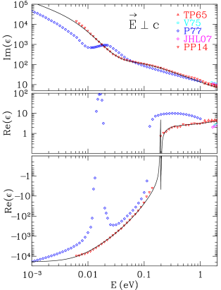
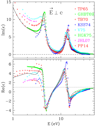
Figure 1: Dielectric function for ${\bf E}\perp\hat{\bf c}$. Solid curve: present model. Data: TP65 = Taft & Philipp (1965), GHBT69=Greenaway et al. (1969), TB70=Tosatti & Bassani (1970), KSS74=Klucker et al. (1974), V75=Venghaus (1975), HGK75=Hagemann et al. (1974, 1975), P77=Philipp (1977), JHL07=Jellison et al. (2007), PP14=Papoular & Papoular (2014). The model $\epsilon_{\perp}$ plotted here is available at http://www.astro.princeton.edu/$\sim$draine/dust/D16graphite/D16graphite.html and http://arks.princeton.edu/ark:/88435/dsp01nc580q118 .

3.2 ${\bf E}\parallel\hat{\bf c}$

Table 3: Component parameters for ${\bf E}\parallel c$

Free-electron-like parameters for ${\bf E}\parallel\hat{\bf c}$
$j$ $A_{j}$ $\hbar\omega_{pj}$ $\omega_{pj}\tau_{{\rm bulk},j}$ $\tau_{{\rm bulk},j}$ $f_{pj}$ $\sigma_{\rm dc}$ $\sigma_{\rm dc}$ (eV) (s) $(10^{12}\,{\rm s}^{-1}$) $\,{\rm mho}{\,{\rm cm}}^{-1}$ 1 1 0.25 0.38 $1.00{\!\,\times\!\,}10^{-15}$ 0.000394 $11.5$ 12.8

Resonance parameters for ${\bf E}\parallel\hat{\bf c}$
$j$ $\hbar\omega_{rj}$ $S_{rj}$ $\gamma_{rj}$ $f_{rj}$ note (eV) 1 0.1075 0.004 0.001 0.0000 Nemanich et al. (1977) 2 4.40 1.4 0.480 0.1713 3 7.20 0.045 0.190 0.0147 4 11.1 0.95 0.120 0.7396 5 12.1 0.21 0.110 0.1943 6 13.5 0.23 0.200 0.2649 7 16.3 0.26 0.210 0.4365 8 22.5 0.20 0.350 0.6397 9 31.0 0.12 0.600 0.7286 10 50.0 0.036 0.700 0.5687 11 100. 0.003 0.700 0.1896 12 200. 0.0001 0.700 0.02527 3.976 total from L shell resonances 2.00 total from K shell 5.976 total

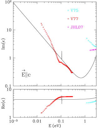
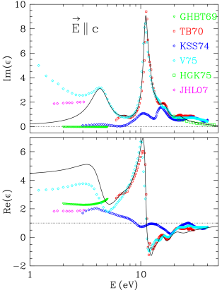
Figure 2: Dielectric function for ${\bf E}\parallel\hat{\bf c}$. Solid curve: present model. Data: GHBT69 = Greenaway et al. (1969), TB70 = Tosatti & Bassani (1970), KSS74 = Klucker et al. (1974), HGK75 = Hagemann et al. (1974, 1975), V75 = Venghaus (1975), V77 = Venghaus (1977), JHL07 = Jellison et al. (2007). The model $\epsilon_{\parallel}$ plotted here is available at http://www.astro.princeton.edu/$\sim$draine/dust/D16graphite/D16graphite.html and http://arks.princeton.edu/ark:/88435/dsp01nc580q118 .

The dielectric function for ${\bf E}\parallel\hat{\bf c}$ is much more uncertain than that for ${\bf E}\perp\hat{\bf c}$. The uncertainty is attributable in part to experimental difficulties, but is likely also due to real sample-to-sample variations, particularly as regards the weak conduction resulting from electrons or holes transiting from one graphene sheet to another.

We adopt free-electron component parameters corresponding to $\sigma_{\rm dc}=12\,{\rm mho}\,{\rm cm}^{-1}$, intermediate between $\sim$$1\,{\rm mho}\,{\rm cm}^{-1}$ (Klein 1962) and $\sim$$200\,{\rm mho}\,{\rm cm}^{-1}$ (Primak 1956) measured for high-quality crystals at $T=300\,{\rm K}$. With a mean-free-time $\tau_{\rm bulk}=1\times 10^{-15}\,{\rm s}$, corresponding to a mean-free-path $v_{\rm F}\tau_{\rm bulk}\approx 4\,{\rm\AA}$ (approximately the interplane spacing), we obtain a free-electron contribution as shown in Figure 2. The adopted free-electron parameters are approximately consistent with the data of Venghaus (1977), which appears to be the only study of $\epsilon_{\parallel}$ in the far-infrared and mid-infrared (see Figure 2).

Graphite has an optically-active out-of-plane lattice resonance at $11.52\micron$ (Nemanich et al. 1977; Jeon & Mahan 2005). We adopt the resonance parameters from Nemanich et al. (1977).

Surprisingly, there do not appear to be published experimental determinations of $\epsilon_{\parallel}$ between 0.3 and 1 eV. At optical frequencies, some studies (Greenaway et al. 1969; Klucker et al. 1974) find negligible absorption [${\rm Im}(\epsilon_{\parallel})\approx 0$] for $2<h\nu<4\,{\rm eV}$, while other investigators (Venghaus 1975; Jellison et al. 2007) report strong absorption [${\rm Im}(\epsilon_{\parallel})\gtrsim 1$] at these energies. Our adopted $\epsilon_{\parallel}$, using 12 resonance-like components (parameters listed in Table 3), has moderately strong absorption in the optical and near-IR, and is reasonably consistent with lab data at higher energies (see Figure 2). Note that $Z_{\rm eff}(\omega\rightarrow\infty)=\sum_{j}f_{pj}+\sum_{j}f_{rj}=3.98$, consistent with the expected sum rule.

4 K Shell Absorption

Absorption by the $1s^{2}$ shell in graphite is also polarization-dependent. Using polarized synchrotron radiation, Rosenberg et al. (1986) measured absorption in a HOPG sample at 7 inclinations of the $c$-axis relative to the polarization. The quantity measured was the electron yield $Y$, including photoelectrons, Auger electrons, and secondary electrons emitted following absorption of an X-ray photon; after subtraction of a “baseline” contributed by absorption by the L shell ($2s^{2}2p^{2}$) electrons, $Y$ is assumed to be proportional to the absorption coefficient contributed by the K shell. Similar measurements of polarization-dependent absorption near the K edge in graphene have also been reported (Pacilé et al. 2008; Papagno et al. 2009).

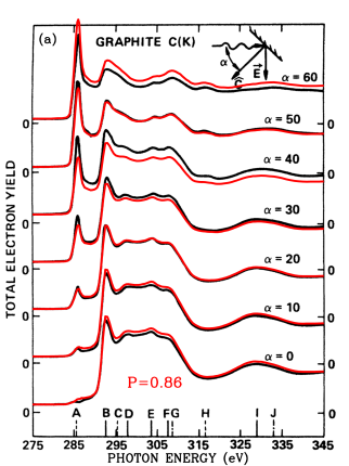
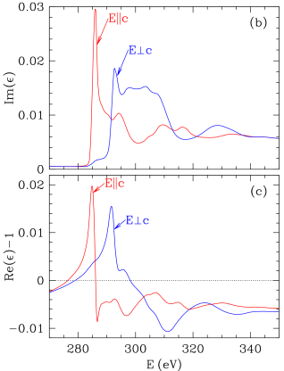
Figure 3: The near-edge X-ray absorption fine structure in graphite has a pronounced dependence on incident polarization. (a) Electron yield $Y(E,\alpha)$ from Rosenberg et al. (1986) with our model (red). (b, c): Our estimate for $\epsilon_{\perp}$ and $\epsilon_{\parallel}$. $\epsilon_{\perp}$ and $\epsilon_{\parallel}$ are available at http://www.astro.princeton.edu/$\sim$draine/dust/D16graphite/D16graphite.html and http://arks.princeton.edu/ark:/88435/dsp01nc580q118 .

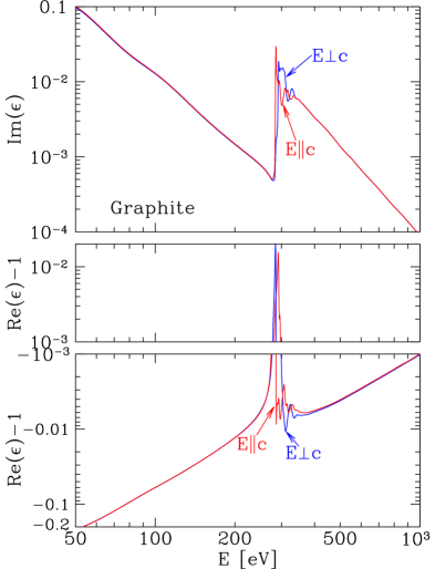
Figure 4: Dielectric tensor for graphite from $50\,{\rm eV}$ to $700\,{\rm eV}$ (see text). From $50$ to $280\,{\rm eV}$ the absorption is due to photoionization from the $2s^{2}2p^{2}$ shell. Above $280\,{\rm eV}$ the absorption is dominated by the electrons in the K shell. $\epsilon_{\perp}$ and $\epsilon_{\parallel}$ are available at http://www.astro.princeton.edu/$\sim$draine/dust/D16graphite/D16graphite.html and http://arks.princeton.edu/ark:/88435/dsp01nc580q118 .

Consider X-rays incident on the graphite basal plane, with $\alpha$ the angle between the incident direction ${\bf k}_{\rm in}$ and the surface normal $\hat{\bf c}$, and assume the incident radiation to have fractional polarization $P$ in the ${\bf k}_{\rm in}-\hat{\bf c}$ plane. If $Y_{\perp}(E)$ and $Y_{\parallel}(E)$ are the yields for incident ${\bf E}\perp\hat{\bf c}$ and ${\bf E}\parallel\hat{\bf c}$, then the yield is the appropriate weighted average of $Y_{\perp}$ and $Y_{\parallel}$:

$$Y(E,\alpha)=\left[\frac{(1+P)}{2}\cos^{2}\alpha+\frac{(1-P)}{2}\right]Y_{\perp}(E)+\left[\frac{(1+P)}{2}\sin^{2}\alpha\right]Y_{\parallel}(E)$$ (12)

where the quantities in square brackets are the fractions of the incident power with ${\bf E}\perp\hat{\bf c}$ and ${\bf E}\parallel\hat{\bf c}$. $Y(E,\alpha)$ from Rosenberg et al. (1986) were used to infer $Y_{\perp}(E)$ and $Y_{\parallel}(E)$ (arbitrary units) for $280\leq E\leq 345\,{\rm eV}$ (see Figure 3a), assuming the incident radiation to have polarization fraction $P=0.86$ (Stöhr & Jaeger 1982). To obtain the contribution $\delta\epsilon_{2}$ of the K shell electrons to $\epsilon_{2}$, we assume that $\omega\delta\epsilon_{2}\propto\delta Y(E)$ where $\delta Y$ is the contribution of the K shell. For $E<345\,{\rm eV}$ we inferred $\delta Y_{\perp},\delta Y_{\parallel}$ from the data of Rosenberg et al. (1986), and set

$${\rm Im}\left(\delta\epsilon_{\rm K}\right)=A\frac{\delta Y(E)}{E}~{}~{}~{}.$$ (13)

For $E>345\,{\rm eV}$ we assumed ${\rm Im}(\delta\epsilon_{\rm K})\propto E^{-4}$ (i.e., absorption coefficient $\propto E^{-3}$). To determine the constant $A$ we require that $\delta\epsilon_{2}$ obey the sum rule (Altarelli et al. 1972)

$$\int_{0}^{\infty}\omega\frac{{\rm Im}(\delta\epsilon_{{\rm K}\parallel}+2\delta\epsilon_{{\rm K}\perp})}{3}d\omega=\frac{2\pi^{2}e^{2}}{m_{e}}Z_{K}n_{\rm C}~{}~{}~{},$$ (14)

where $Z_{K}=2$ is the number of K shell electrons per C, and $n_{\rm C}$ is the number density of C atoms. ${\rm Re}(\delta\epsilon_{\rm K})$ is obtained from ${\rm Im}(\delta\epsilon_{\rm K})$ using the Kramers-Kronig relation (1). Combining $\delta\epsilon_{K}(\omega)$ with the free-electron and resonance model (see Eq. 2) yields a dielectric tensor for graphite extending continuously from $0$ to $10\,{\rm keV}$. The resulting $\epsilon_{\perp}$ and $\epsilon_{\parallel}$ are shown in Figure 3b,c. The near-edge absorption is strongly polarization-dependent: For ${\bf E}\parallel\hat{\bf c}$ the absorption peaks at 286$\,{\rm eV}$, whereas for ${\bf E}\perp\hat{\bf c}$ the absorption peaks at 293$\,{\rm eV}$.

Figure 4 shows the dielectric function from $50\,{\rm eV}$ to $1\,{\rm keV}$. Between $50\,{\rm eV}$ and $280\,{\rm eV}$ the absorption is smooth and featureless, arising from photoionization of the 4 electrons in the L shell. At $\sim$$282\,{\rm eV}$ the onset of K shell absorption causes ${\rm Im}(\epsilon)$ to increase by a factor $\sim$50. For energies $E\gtrsim 350\,{\rm eV}$, the photolectric opacity declines smoothly with increasing energy.

Figure 5 shows the effective number $n_{\rm eff}(E)$ of electrons contributing to absorption at $\hbar\omega\leq E$ for $\epsilon_{\perp}$ and $\epsilon_{\parallel}$.

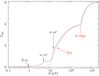
Figure 5: $Z_{\rm eff}(E)$, the effective number of electrons per C producing absorption at $\hbar\omega\leq E$ (see Eq. 5) for $\epsilon_{\perp}$ and $\epsilon_{\parallel}$.

5 Absorption and Scattering by Single-Crystal Spheres and Spheroids

Consider a spheroid with semi-axes $(a,b,b)$, composed of a uniaxial material such as graphite. Assume $\hat{\bf c}\parallel\hat{\bf a}$, where $\hat{\bf c}$ is the crystal $c$-axis and $\hat{\bf a}$ is the spheroid symmetry axis. The volume $V=(4\pi/3)ab^{2}$, and $a_{\rm eff}\equiv(ab^{2})^{1/3}$ is the radius of an equal-volume sphere.

Calculation of absorption and scattering by particles composed of anisotropic materials is a difficult problem, even for spheres. Accurate calculation of $C_{\rm abs}$ and $C_{\rm sca}$ requires solving Maxwell’s equations for an incident plane wave interacting with the target, using a method that can explicitly treat anisotropic materials. While certain approximations (see §5.2) can be used when $a_{\rm eff}/\lambda\ll 1$, analytic treatments of the general case are lacking, and we are forced to rely on numerical methods.

5.1 Accurate Results: the Discrete Dipole Approximation

The discrete dipole approximation (DDA) (Purcell & Pennypacker 1973; Draine 1988; Draine & Flatau 1994) can explicitly treat anisotropic dielectric tensors and nonspherical target geometries. Anisotropic dielectric tensors are treated by assigning to each dipole a polarizability tensor with the polarization response depending on the direction of the local electric field relative to the local crystalline axes. The DDA results are expected to converge to the exact solution to Maxwell’s equations in the limit $N\rightarrow\infty$, where $N$ is the number of dipoles used to represent the target. Draine & Malhotra (1993) used the DDA to show that the $\nicefrac{{1}}{{3}}$ - $\nicefrac{{2}}{{3}}$ approximation was reasonably accurate for $a\lesssim 0.04\micron$ graphite spheres in the vacuum ultraviolet. However, validity of the $\nicefrac{{1}}{{3}}$ - $\nicefrac{{2}}{{3}}$ approximation for larger particles, or at optical and near-infrared wavelengths, does not appear to thus far have been investigated.

We use the DDA code DDSCAT 7.3.1 to calculate scattering and absorption by randomly-oriented graphite spheres and spheroids of various sizes. For spheroids, we assume $\hat{\bf c}\parallel\hat{\bf a}$. Let $\Theta$ be the angle between the incident ${\bf k}$ and $\hat{\bf a}$; the angular average $\langle C\rangle=\int_{0}^{1}C(\Theta)d\cos\Theta$ is evaluated using Simpson’s rule and 5 values of $\cos\Theta=0,0.25,0.5,0.75,1$. For each $\Theta$, we average over incident polarizations. We obtain dimensionless efficiency factors $Q_{\rm ext}(\lambda)\equiv C_{\rm ext}(\lambda)/\pi a_{\rm eff}^{2}$.

The DDA is exact in the limit $N\rightarrow\infty$. For sufficiently large $N$, it is expected that the DDSCAT error will scale as $N^{-1/3}$. This scaling law is expected intuitively ($N^{-1/3}\propto$ the fraction of the dipoles that are located on the surface of the target) and has been verified computationally (see, e.g. Collinge & Draine 2004). Thus we expect

$$Q_{N}\approx Q_{\infty}+AN^{-1/3}~{}~{}~{},$$ (15)

and we can therefore estimate the “exact” result from calculations with $N=N_{1}$ and $N_{2}$:

$$Q_{\infty} \approx Q_{N_{2}}\times\left(1-\phi_{N_{2}}\right)$$ (16)

$$\phi_{N_{2}} \equiv \frac{Q_{N_{1}}/Q_{N_{2}}-1}{(N_{2}/N_{1})^{1/3}-1}~{}~{}~{},$$ (17)

and the coefficient $A$ in Eq. (15) is

$$A=\frac{(Q_{N_{2}}-Q_{N_{1}})N_{2}^{1/3}}{1-(N_{2}/N_{1})^{1/3}}=Q_{N_{2}}\times\phi_{N_{2}}\times\left(\frac{N_{1}}{N_{2}}\right)^{1/3}~{}~{}~{}.$$ (18)

In practice, one chooses as large a value of $N_{2}$ as is computationally feasible, and then chooses a value of $N_{1}\lesssim N_{2}/2$. If we simply took $Q_{N_{2}}$ as our estimate for the exact result $Q_{\infty}$, the fractional error would be $\phi_{N_{2}}$. Because (15) is expected to closely describe the dependence on $N$, the extrapolation (16) should yield an estimate for the exact result $Q_{\infty}$ with a fractional error much smaller than $\phi_{N_{2}}$, where $N_{2}$ is the largest value of $N$ for which converged DDA results are available. As a simple rule-of-thumb, we suggest that $Q_{N_{2}}\times(1-\phi_{N_{2}})$ will approximate the “exact” result $Q_{\infty}$ to within a fractional error $\sim$$0.1\phi_{N_{2}}$.

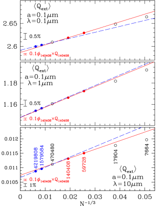
Figure 6: Convergence of DDA results for $\langle Q_{\rm ext}\rangle$ as $N^{-1/3}\rightarrow 0$ for $a=0.1\micron$ single-crystal graphite sphere and $\lambda=0.1,1,10\micron$. The red line is Eq. (15) fitted to the results for $N_{1}=59708$ and $N_{2}=140408$ (red points). Red vertical bars show $0.1\phi_{140408}Q_{140408}$, the estimated uncertainty in the extrapolation to $N=\infty$ from results for $N_{1}=59708$ and $N_{2}=140408$. The broken blue line is Eq. (15) fitted to the results for $N_{1}=1.58\times 10^{6}$ and $N_{2}=4.22\times 10^{6}$. Black vertical bars show shifts of 1% and 0.5%. Eq. (16) allows reliable extrapolation to $N\rightarrow\infty$ provided $N_{1},N_{2}$ are sufficiently large, with estimated fractional uncertainty $\sim$$0.1\phi_{N_{2}}$.

In Figure 6 we show results calculated for $a=0.1\micron$ graphite spheres at 3 wavelengths: $\lambda=10\micron$, $1\micron$, and $0.1\micron$. For each case the DDA calculations were done with 7 different values of $N$, ranging from $N\!=\!7664$ to $N\!=\!4.22{\!\,\times\!\,}10^{6}$. The solid line is Eq. (15) fitted to the results for $N_{1}\!=\!59708$ and $N_{2}\!=\!140408$, and the dashed line is Eq. (15) fitted to the results for $N_{1}\!=\!1.58{\!\,\times\!\,}10^{6}$ and $N_{2}\!=\!4.22{\!\,\times\!\,}10^{6}$. We see that the numerical results conform quite well to the functional form (15), with $\sim$$0.1\phi_{N_{2}}$ providing a reasonable estimate for the uncertainty in the extrapolation to the exact result.

To survey many combinations of $(a,\lambda)$ we consider $0.005\micron\leq a_{\rm eff}\leq 0.3\micron$ and $10\micron\geq\lambda\geq 0.1\micron$ (scattering parameter $x\equiv 2\pi a_{\rm eff}/\lambda$ ranging from $0.00314$ to $18.85$). Figure 7 shows fully-anisotropic DDA calculations of $\langle Q_{\rm ext}\rangle$ for randomly-oriented single-crystal graphite spheres. The circles are the DDA results for $N=140408$ dipoles, and the solid curves are the DDA results extrapolated to $N=\infty$ using Eq. (16). The fractional adjustments $\phi_{N}$ are generally quite small, so that the curves appear to coincide with the circles. The upper panel shows $\phi_{N}$ for 4 different values of $a$, for $N=140408$. For all cases shown in Figure 7, $|\phi_{N}|<0.07$ for $N=140408$.

The extrapolation (16) is expected to provide an estimate for $Q_{\infty}$ accurate to a fraction of $\phi_{N}$; hence we consider that the extrapolations to $N\rightarrow\infty$ in Figure 7 should be accurate to $\sim 1\%$ or better. The DDA – which fully allows for anisotropic dielectric tensors – can therefore be used as the “gold standard” to test other, faster, approximation methods, such as the “$\nicefrac{{1}}{{3}}$ - $\nicefrac{{2}}{{3}}$” approximation.

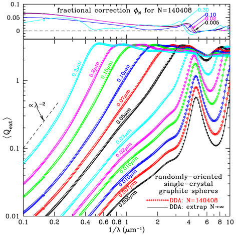
Figure 7: Lower panel: $\langle Q_{\rm ext}(\lambda)\rangle$ for randomly-oriented graphite spheres, calculated with the DDA with the anisotropic dielectric tensor of graphite, for radii from $0.005\micron$ to $0.3\micron$. DDA results are shown for $N=140408$ dipoles (circles) and the extrapolation to $N\rightarrow\infty$ using results for $N_{1}=59728$ and $N_{2}=140408$ (solid curves). Upper panel: the fractional difference $\phi_{N}$ between the DDA results for $N=140408$ and the $N\rightarrow\infty$ extrapolation, for 4 selected radii (indicated). The fractional uncertainty in the DDA extrapolation is $\sim$$0.1\phi_{N}$, i.e., less than 1% for all cases shown. DDA cross sections plotted here are available at http://www.astro.princeton.edu/$\sim$draine/dust/D16graphite/D16graphite.html and http://arks.princeton.edu/ark:/88435/dsp01nc580q118 .

5.2 The $\nicefrac{{1}}{{3}}$ - $\nicefrac{{2}}{{3}}$ Approximation

If the particle is small compared to the wavelength, an accurate analytic approximation is available for homogeneous spheres, spheroids, and ellipsoids, even when composed of anisotropic materials. Here we consider spheroids composed of uniaxial material (such as graphite) with the crystal axis $\hat{\bf c}$ parallel to the spheroid symmetry axis $\hat{\bf a}$. If $a_{\rm eff}\ll\lambda\equiv 2\pi c/\omega$, the electric dipole approximation (Draine & Lee 1984) can be used to calculate absorption and scattering cross sections:

$$C_{\rm abs} = |\hat{\bf e}\cdot\hat{\bf a}|^{2}C_{\rm abs}^{\rm(ed)}(\epsilon_{\parallel},L_{a})+\left(1-|\hat{\bf e}\cdot\hat{\bf a}|^{2}\right)C_{\rm abs}^{\rm(ed)}(\epsilon_{\perp},L_{b})$$ (19)

$$C_{\rm sca} = |\hat{\bf e}\cdot\hat{\bf a}|^{2}C_{\rm sca}^{\rm(ed)}(\epsilon_{\parallel},L_{a})+\left(1-|\hat{\bf e}\cdot\hat{\bf a}|^{2}\right)C_{\rm sca}^{\rm(ed)}(\epsilon_{\perp},L_{b})~{}~{}~{},$$ (20)

where $\hat{\bf e}$ is the incident polarization unit vector,

$$C_{\rm abs}^{\rm(ed)}(\epsilon,L) = \frac{2\pi V}{\lambda}\frac{\epsilon_{2}}{\left|1+(\epsilon-1)L\right|^{2}}$$ (21)

$$C_{\rm sca}^{\rm(ed)}(\epsilon,L) = \frac{8\pi^{3}V^{2}}{3\lambda^{4}}\left|\frac{\epsilon-1}{1+(\epsilon-1)L}\right|^{2}~{}~{}~{},$$ (22)

are the “electric dipole” cross sections calculated for spheroids of volume $V$ with isotropic dielectric function $\epsilon$, and $L_{a}$ and $L_{b}=(1-L_{a})/2$ are the usual “shape factors” for spheroids.

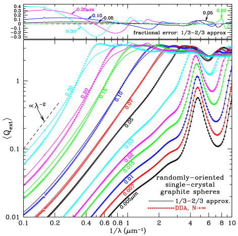
Figure 8: Lower panel: $\langle Q_{\rm ext}(\lambda)\rangle$ for randomly-oriented single-crystal graphite spheres with indicated radii $a$, calculated with the $\nicefrac{{1}}{{3}}$ - $\nicefrac{{2}}{{3}}$ approximation (solid lines) and extrapolated from DDA calculations with $N_{1}=59708$, $N_{2}=140408$ (open circles; see solid curves in Fig. 7). Upper panel: fractional error resulting from the $\nicefrac{{1}}{{3}}$ - $\nicefrac{{2}}{{3}}$ approximation. For $a=0.3\micron$, the $\nicefrac{{1}}{{3}}$ - $\nicefrac{{2}}{{3}}$ approximation overpredicts $\langle Q_{\rm ext}\rangle$ by 40% at $\lambda=10\micron$, and underpredicts $\langle Q_{\rm ext}\rangle$ by 30% at $\lambda=2\micron$.

Randomly-oriented spheroids have $\langle|\hat{\bf e}\cdot\hat{\bf a}|^{2}\rangle=1/3$, and the average cross section per particle in the electric dipole limit is simply

$$\langle C_{\rm abs}\rangle = \frac{1}{3}C_{\rm abs}^{\rm(ed)}(\epsilon_{\parallel},L_{a})+\frac{2}{3}C_{\rm abs}^{\rm(ed)}(\epsilon_{\perp},L_{b})$$ (23)

$$\langle C_{\rm sca}\rangle = \frac{1}{3}C_{\rm sca}^{\rm(ed)}(\epsilon_{\parallel},L_{a})+\frac{2}{3}C_{\rm sca}^{\rm(ed)}(\epsilon_{\perp},L_{b})~{}~{}~{}.$$ (24)

This is known as the “$\nicefrac{{1}}{{3}}$ - $\nicefrac{{2}}{{3}}$ approximation”. For crystalline spheres, or for crystalline spheroids with $\hat{\bf a}\parallel\hat{\bf c}$ or $\hat{\bf a}\perp\hat{\bf c}$, the $\nicefrac{{1}}{{3}}$ - $\nicefrac{{2}}{{3}}$ approximation is exact in the limit $a/\lambda\rightarrow 0$ because small particles are then in the “electric dipole limit”, where the particle’s response to radiation can be fully characterized by the induced electric dipole moment (Draine & Lee 1984).

The $\nicefrac{{1}}{{3}}$ - $\nicefrac{{2}}{{3}}$ approximation,

$$\langle C_{\rm abs}\rangle\approx\frac{1}{3}C_{\rm abs}^{\rm(iso)}(\epsilon_{\parallel})+\frac{2}{3}C_{\rm abs}^{\rm(iso)}(\epsilon_{\perp})$$ (25)

is frequently used even when $a/\lambda$ is not small, where now $C^{\rm(iso)}(\epsilon)$ is a cross section calculated for the same shape with an isotropic dielectric function $\epsilon$. The $\nicefrac{{1}}{{3}}$ - $\nicefrac{{2}}{{3}}$ weighting of $C^{\rm(iso)}$ calculated for two different dielectric functions seems plausible as an approximation, but there have been few tests of its accuracy.

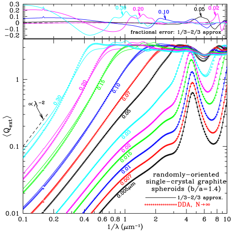
Figure 9: Lower panel: $\langle Q_{\rm ext}(\lambda)\rangle$ for oblate single-crystal graphite spheroids, axial ratio $b/a=1.4$, with symmetry axis $\hat{\bf a}\parallel\hat{\bf c}$. Effective radii $a_{\rm eff}\equiv(ab^{2})^{1/3}$ are indicated. Circles: $N\rightarrow\infty$ extrapolation from DDA calculations with $N_{1}=60476$ and $N_{2}=131040$ dipoles. Solid lines: Theory for isotropic spheroids (Voshchinnikov & Farafonov 1993) using the $\nicefrac{{1}}{{3}}$ - $\nicefrac{{2}}{{3}}$ approximation (see text). Upper panel: fractional error in the $\nicefrac{{1}}{{3}}$ - $\nicefrac{{2}}{{3}}$ approximation for selected radii (indicated). DDA cross sections plotted here are available at http://www.astro.princeton.edu/$\sim$draine/dust/D16graphite/D16graphite.html and http://arks.princeton.edu/ark:/88435/dsp01nc580q118 .

Figure 8 tests the $\nicefrac{{1}}{{3}}$ - $\nicefrac{{2}}{{3}}$ approximation for spheres. The points show the “exact” results from Fig. 7 obtained using the DDA for radii between $0.005\micron$ and $0.3\micron$ and wavelengths between $10$ and $0.1\micron$. The solid curves in Figure 8 show the predictions of the $\nicefrac{{1}}{{3}}$ - $\nicefrac{{2}}{{3}}$ approximation with Mie theory used to evaluate $C_{\rm ext}^{\rm(iso)}$. The upper panel in Fig. 8 shows the fractional error resulting from use of the $\nicefrac{{1}}{{3}}$ - $\nicefrac{{2}}{{3}}$ approximation, for selected radii. Over the surveyed domain ($a\leq 0.3\micron$, $0.1\leq\lambda\leq 10\micron$) the largest errors occur near $10\micron$ ($E\approx 0.1\,{\rm eV}$), where $|\epsilon_{\perp}|$ is becoming large (see Figure 1).

As expected, the $\nicefrac{{1}}{{3}}$ - $\nicefrac{{2}}{{3}}$ approximation is highly accurate in the limit $a/\lambda\rightarrow 0$, but the errors are generally $\lesssim 10\%$ in the optical and UV, even when $a/\lambda$ is not small. Relatively large errors occur for $a/\lambda\approx 0.15$ (i.e., $2\pi a/\lambda\approx 1$) where the $\nicefrac{{1}}{{3}}$ - $\nicefrac{{2}}{{3}}$ approximation tends to underestimate $\langle Q_{\rm ext}\rangle$. For example, for $a=0.1\micron$ graphite spheres, the $\nicefrac{{1}}{{3}}$ - $\nicefrac{{2}}{{3}}$ approximation underestimates $Q_{\rm ext}$ by 12% at $\lambda={0.6}\micron$ ($\lambda^{-1}=1.5\micron^{-1}$). Errors at $a/\lambda\approx 0.15$ are probably of greatest importance, because for size distributions in the ISM (e.g., the MRN power law $dn/da\propto a^{-3.5}$, $a\lesssim 0.25\micron$) and $0.1\micron\lesssim\lambda\lesssim 2\micron$, the grains with $a\approx 0.15\lambda$ tend to dominate the extinction at wavelength $\lambda$. At longer wavelengths, the graphite dielectric tensor becomes large, especially $\epsilon_{\perp}$ (see Figs. 1 and 2), and the errors for given $a/\lambda$ tend to increase. For $a/\lambda=0.15$, the $\nicefrac{{1}}{{3}}$ - $\nicefrac{{2}}{{3}}$ approximation underestimates $Q_{\rm ext}$ by $\sim$30% at $\lambda=2\micron$. The $\nicefrac{{1}}{{3}}$ - $\nicefrac{{2}}{{3}}$ approximation overestimates $\langle Q_{\rm ext}\rangle$ by 40% for $a=0.30\micron$ at $\lambda=10\micron$, even though $a/\lambda=0.03$ is small.

Figure 9 shows $\langle Q_{\rm ext}\rangle$ for single-crystal oblate spheroids with axial ratio $b/a=1.4$. The graphite $c$-axis is assumed to be parallel to the symmetry axis of the spheroid. $\langle C_{\rm ext}\rangle$ for randomly-oriented spheroids is obtained by averaging DDA calculations of $C_{\rm ext}=C_{\rm abs}+C_{\rm sca}$ for 5 different orientations ($\cos\Theta=0,0.25,0.5,0.75,1$) of the grain relative to the incident direction of propagation $\hat{\bf k}$, extrapolating to $N\rightarrow\infty$ from results computed for $N_{1}=60476$ and $N_{2}=131040$.

Absorption and scattering cross sections were also calculated using the spheroid code of Voshchinnikov & Farafonov (1993) and the $\nicefrac{{1}}{{3}}$ - $\nicefrac{{2}}{{3}}$ approximation, using 3 grain orientations:

$$\langle C_{\rm ext}\rangle\approx\frac{1}{3}C_{\rm ext}^{\rm(iso)}(\hat{\bf k}\!\parallel\!\hat{\bf a},\hat{\bf e}\!\perp\!\hat{\bf a},\epsilon_{\perp})+\frac{1}{3}C_{\rm ext}^{\rm(iso)}(\hat{\bf k}\!\perp\!\hat{\bf a},\hat{\bf e}\!\perp\!\hat{\bf a},\epsilon_{\perp})+\frac{1}{3}C_{\rm ext}^{\rm(iso)}(\hat{\bf k}\!\perp\!\hat{\bf a},\hat{\bf e}\!\parallel\!\hat{\bf a},\epsilon_{\parallel})~{}~{}~{},$$ (26)

where $C^{\rm(iso)}(\hat{\bf k},\hat{\bf e},\epsilon)$ is the cross section for the same shape target but with an isotropic dielectric function $\epsilon$. From Fig. 9 we see that for $b/a=1.4$ the Voshchinnikov & Farafonov (1993) spheroid code plus the $\nicefrac{{1}}{{3}}$ - $\nicefrac{{2}}{{3}}$ approximation yields estimates for $\langle Q_{\rm ext}\rangle$ that are accurate to within 15% for $\lambda<0.9\micron$. The errors come from the $\nicefrac{{1}}{{3}}$ - $\nicefrac{{2}}{{3}}$ aproximation, as seen from the similar errors for spheres in Fig. 8. Once again: (1) the $\nicefrac{{1}}{{3}}$ - $\nicefrac{{2}}{{3}}$ approximation tends to underestimate $C_{\rm ext}$ for $a_{\rm eff}/\lambda\approx 0.15$; (2) the errors are $\lesssim$10% in the optical-UV; (3) for given $a/\lambda$, the fractional errors increase at long wavelengths, as $\epsilon_{\perp}$ becomes large. While accurate DDA computations are preferred, the fact that the $\nicefrac{{1}}{{3}}$ - $\nicefrac{{2}}{{3}}$ approximation is exact for $a/\lambda\rightarrow 0$, and moderately accurate for all $a/\lambda$, allows it to be used when DDA computations would be infeasible.

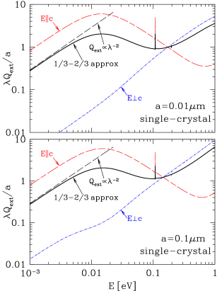
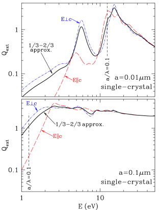
Figure 10: Solid line: $Q_{\rm ext}$ for randomly-oriented single-crystal graphite spheres, calculated using Mie theory with the $\nicefrac{{1}}{{3}}$ - $\nicefrac{{2}}{{3}}$ approximation, for radii $a=0.01\micron$ and $0.1\micron$. The $\nicefrac{{1}}{{3}}$ - $\nicefrac{{2}}{{3}}$ approximation is expected to be accurate for $a/\lambda\lesssim 0.1$ (to the left of the vertical dashed lines), but for larger values of $a/\lambda$ its accuracy is uncertain (but see Fig. 8). Dashed and dash-dot curves are $Q_{\rm ext}$ calculated using $\epsilon_{\perp}$ and $\epsilon_{\parallel}$. These cross sections, and results for other sizes, are available at http://www.astro.princeton.edu/$\sim$draine/dust/D16graphite/D16graphite.html and http://arks.princeton.edu/ark:/88435/dsp01nc580q118 .

Having established that the $\nicefrac{{1}}{{3}}$ - $\nicefrac{{2}}{{3}}$ approximation is moderately accurate for all $\lambda$, we now use it to calculate cross sections for single-crystal graphite spheres over a broad range of wavelengths and sizes. Figure 10 shows extinction cross sections calculated for (1) isotropic spheres with $\epsilon=\epsilon_{\perp}$; (2) isotropic spheres with $\epsilon=\epsilon_{\parallel}$; (3) the $\nicefrac{{1}}{{3}}$ - $\nicefrac{{2}}{{3}}$ approximation (the weighted sum of the above two curves).

We see that for $E\lesssim 0.1\,{\rm eV}$ ($\lambda>10\micron$), the absorption is primarily due to the component with ${\bf E}\parallel\hat{\bf c}$ – the conductivity for ${\bf E}\perp\hat{\bf c}$ is so large that the currents driven by the applied ${\bf E}$ don’t result in as much dissipation as is associated with the ${\bf E}\parallel\hat{\bf c}$ component. For $\lambda\gtrsim 200\micron$ the graphite opacity has the “classical” $Q_{\rm abs}\propto\lambda^{-2}$ behavior.

6 Turbostratic Graphite and Effective Medium Theory

“Turbostratic graphite” refers to material with the short-range order of graphite, but with randomly-oriented microcrystallites (Mrozowski 1971; Robertson 1986). Highly-aromatized amorphous carbon would be in this category. Papoular & Papoular (2009, hereafter PP09) argue that turbostratic graphite (which they refer to as “polycrystalline graphite”) in very small ($a\lesssim 0.01\micron$) particles could account for the observed 2175Å extinction band. Some of the isotopically-anomalous presolar graphite grains found in meteorites are composed of turbostratic graphite (Croat et al. 2008; Zinner 2014). If interstellar grains contain a carbonaceous component that is highly aromatic but lacking in long-range order, the optical properties may be similar to turbostratic graphite.

In principle, the DDA can be used to calculate the response from grains composed of turbostratic graphite, but such calculations are numerically very challenging because of the need to employ sufficient dipoles to mimic the arrangement of the microcrystallites, whatever that may be thought to be. In the absence of such direct brute-force calculations, one approach is to employ “effective medium theory” (EMT) to try to obtain an “effective” isotropic dielectric function $\epsilon_{\rm eff}$ for turbostratic graphite, and then calculate scattering and absorption for homogeneous grains with $\epsilon=\epsilon_{\rm eff}$.

A number of different EMTs have been proposed (see, e.g., Bohren & Huffman 1983).

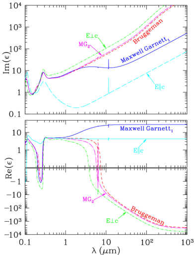
Figure 11: Components $\epsilon_{\parallel}$ and $\epsilon_{\perp}$ of the graphite dielectric tensor, together with effective dielectric functions for turbostratic graphite obtained from the Maxwell Garnett and Bruggeman treatments (see text). The MG₁ dielectric function is available from http://www.astro.princeton.edu/$\sim$draine/dust/D16graphite/D16graphite.html and http://arks.princeton.edu/ark:/88435/dsp01nc580q118 .

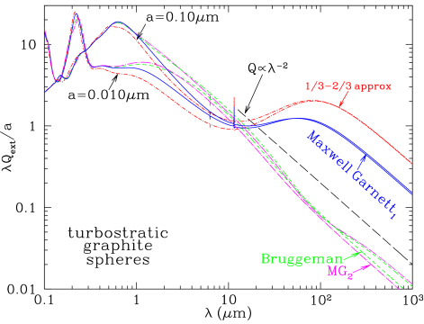
Figure 12: Solid curves: $Q_{\rm ext}$ for turbostratic graphite grains, estimated using Maxwell Garnett EMTs MG₁ and MG₂, for $a=0.01\micron$ and $a=0.10\micron$. Also shown are estimates from the $\nicefrac{{1}}{{3}}$ - $\nicefrac{{2}}{{3}}$ approximation (dot-dashed) and the Bruggeman EMT (dashed). For $\lambda\lesssim 10\micron$ the $\nicefrac{{1}}{{3}}$ - $\nicefrac{{2}}{{3}}$ approximation and all EMTs give similar estimates for $Q_{\rm ext}$, but for $\lambda>30\micron$ the estimates can differ by factors of $\sim$2 or more. We recommend the MG₁ EMT (see text).

In the approach of Bruggeman the two components are treated symmetrically, with filling factors $\nicefrac{{1}}{{3}},\nicefrac{{2}}{{3}}$ for $\epsilon_{\parallel},\epsilon_{\perp}$. The Bruggeman estimate $\epsilon_{\rm B}$ for the effective dielectric function is determined by

$$0=\frac{1}{3}\frac{(\epsilon_{\parallel}-\epsilon_{\rm B})}{(\epsilon_{\parallel}+2\epsilon_{\rm B})}+\frac{2}{3}\frac{(\epsilon_{\perp}-\epsilon_{\rm B})}{(\epsilon_{\perp}+2\epsilon_{\rm B})}~{}~{}~{},$$ (27)

with solution

$$\epsilon_{\rm B}=\frac{1}{4}\left[\epsilon_{\perp}+\left(\epsilon_{\perp}^{2}+8\epsilon_{\parallel}\epsilon_{\perp}\right)^{1/2}\right]~{}~{}~{}.$$ (28)

The Bruggeman EMT was used by PP09 to model turbostratic graphite grains.

The approach of Maxwell Garnett (1904) is often used, where the composite medium is treated as a “matrix” (with dielectric function $\epsilon_{\rm matr}$) containing inclusions (with dielectric function $\epsilon_{\rm incl}$ and volume filling factor $f_{\rm incl}$. If the inclusions are taken to be spherical, the Maxwell Garnett estimate for the effective dielectric function is

$$\epsilon_{\rm MG}=\epsilon_{\rm matr}\frac{[3\epsilon_{\rm matr}+(1+2f_{\rm incl})(\epsilon_{\rm incl}-\epsilon_{\rm matr})]}{[3\epsilon_{\rm matr}+(1-f_{\rm incl})(\epsilon_{\rm incl}-\epsilon_{\rm matr})]}~{}~{}~{}.$$ (29)

Because the two materials are treated asymmetrically, it is necessary to identify one as the matrix and the other as the inclusion. As our standard “Maxwell Garnett EMT” for turbostratic graphite we will take $\epsilon_{\rm matr}=\epsilon_{\parallel}$, $\epsilon_{\rm incl}=\epsilon_{\perp}$, and $f_{\rm incl}=2/3$. Thus,

$$\epsilon_{\rm MG_{1}}=\epsilon_{\parallel}\left[\frac{2\epsilon_{\parallel}+7\epsilon_{\perp}}{8\epsilon_{\parallel}+\epsilon_{\perp}}\right]~{}~{}~{}.$$ (30)

However, we will also examine the consequences of reversing the choices of matrix and inclusion, and will consider $\epsilon_{\rm matr}=\epsilon_{\perp}$, $\epsilon_{\rm incl}=\epsilon_{\parallel}$, and $f_{\rm incl}=1/3$:

$$\epsilon_{\rm MG_{2}}=\epsilon_{\perp}\left[\frac{5\epsilon_{\parallel}+4\epsilon_{\perp}}{2\epsilon_{\parallel}+7\epsilon_{\perp}}\right]~{}~{}~{}.$$ (31)

Figure 11 shows $\epsilon_{\rm B}$, $\epsilon_{\rm MG_{1}}$, and $\epsilon_{\rm MG_{2}}$ derived from the graphite dielectric tensor components $\epsilon_{\parallel}$ and $\epsilon_{\perp}$. At wavelengths $\lambda<1\micron$, $\epsilon_{\rm MG}$, $\epsilon_{\rm MG_{2}}$, and $\epsilon_{\rm B}$ are seen to be nearly identical, but at long wavelengths $\epsilon_{\rm MG_{1}}$ differs greatly from $\epsilon_{\rm MG_{2}}$ and $\epsilon_{\rm B}$. Note that because $\epsilon_{\rm MG_{1}}$, $\epsilon_{\rm MG_{2}}$, and $\epsilon_{\rm B}$ are all analytic functions of $\epsilon_{\parallel}$ and $\epsilon_{\perp}$ (see Eqs. 28, 30 and 31), it follows (see Bohren 2010) that $\epsilon_{\rm MG_{1}}(\omega)$, $\epsilon_{\rm MG_{2}}(\omega)$, and $\epsilon_{\rm B}(\omega)$ each satisfies the Kramers-Kronig relations.

Abeles & Gittleman (1976) found the Maxwell Garnett EMT to be more successful than the Bruggeman EMT in characterizing the optical properties of “granular metals”, such as sputtered Ag-SiO₂ films, with the insulator SiO₂ treated as the “matrix” and the Ag treated as the inclusion, even for Ag filling factors $f_{\rm incl}\rightarrow 1$. This version of the Maxwell Garnett EMT was also found to be in better agreement with measurements on “granular semiconductors”, such as Si-SiC, with the stronger absorber (SiC near the SiC stretching mode at 12.7$\micron$) treated as the inclusion. This suggests that $\epsilon_{\rm MG_{1}}$ – which treats the more-strongly-absorbing $\epsilon_{\perp}$ component as the inclusion – may be the better estimator for turbostratic graphite.

Figure 12 shows cross sections for turbostratic graphite spheres calculated using these three different EMTs. For comparison, $\langle Q_{\rm ext}\rangle$ is also shown for randomly-oriented single-crystal spheres, calculated using the $\nicefrac{{1}}{{3}}$ - $\nicefrac{{2}}{{3}}$ approximation. For $\lambda\lesssim 1\micron$ the $\nicefrac{{1}}{{3}}$ - $\nicefrac{{2}}{{3}}$ approximation and the two EMT variants all give comparable estimates for $\langle Q_{\rm ext}\rangle$. However, for $\lambda\gtrsim 20\micron$ the estimates diverge.

For turbostratic graphite, we might expect the absorption at long wavelengths to be less than given by the $\nicefrac{{1}}{{3}}$ - $\nicefrac{{2}}{{3}}$ approximation, because the high conductivity for ${\bf E}\perp\hat{\bf c}$ allows it to “screen” the regions characterized by $\epsilon_{\parallel}$ from the electric field of the incident wave. For $\lambda\gtrsim 100\micron$, the Bruggeman or MG₂ EMTs both result in an order of magnitude greater suppression of absorption than does our “standard” Maxwell Garnett approach with $\epsilon_{\perp}$ inclusions.

The submicron grains in the ISM have typical sizes $\sim 0.1\micron$. If the microcrystals are more-or-less randomly-oriented, with similar dimensions parallel and perpendicular to $\hat{\bf c}$, then we might expect $\sim 1/3$ of the surface area of the grain to consist of “basal plane”. These microcrystals will not be shielded from incident electric fields that are more-or-less normal to the grain surface, and thus these “exposed basal-plane” microcrystals would contribute to absorption. If the microcrystal dimensions are $\sim 0.01\micron$, then a significant fraction $\sim 0.3$ of the grain volume is contributed by microcrystals at the grain surface. We might then expect the far-infrared absorption cross section of such a particle to be $\sim 30\%$ as large as estimated by the $\nicefrac{{1}}{{3}}$ - $\nicefrac{{2}}{{3}}$ approximation for a single-crystal grain – this happens to be about what our “standard” Maxwell Garnett approximation (MG₁) gives (see Figure 12). Further note that there may be a tendency for microcrystals near the surface to preferentially orient with their basal planes $\sim$parallel to the grain surface, as in the onion-like presolar graphite grains found in primitive meteorites (see, e.g., Bernatowicz et al. 1996), in which case the $\epsilon_{\parallel}$ component would be able to contribute to the absorption without intervening “shielding” by $\epsilon_{\perp}$.

Neither the Bruggeman nor the Maxwell Garnett approaches are theoretically compelling. Based on the above discussion, we tentatively recommend the MG₁ estimate (30) for the effective dielectric function of turbostratic graphite grains, but it must be recognized that this is uncertain. Theoretical progress on this question appears to require ambitious calculations using the DDA to solve for the electromagnetic field within turbostratic graphite structures. The feasibility of such calculations is uncertain because $\epsilon_{\parallel}$ and especially $\epsilon_{\perp}$ become numerically large at wavelengths $\lambda\gtrsim 10\micron$, making DDA calculations especially challenging. Alternatively, lab measurements of turbostratic graphite grain opacities at wavelengths $\gtrsim 30\micron$ could determine whether they agree better with the the Bruggeman and MG₂ predictions or the order-of-magnitude larger opacities predicted by the MG₁ EMT.

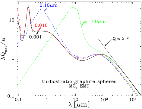
Figure 13: Extinction cross sections for turbostratic graphite spheres with selected radii $a=0.001\micron$, $0.01\micron$, $0.1\micron$, and $1\micron$. Tabulated results for these and other sizes are available at http://www.astro.princeton.edu/$\sim$draine/dust/D16graphite/D16graphite.html and http://arks.princeton.edu/ark:/88435/dsp01nc580q118 .

7 Cross Sections for Turbostratic Graphite Spheres and Spheroids

Adopting the Maxwell Garnett EMT (30) to estimate an effective dielectric function $\epsilon_{\rm MG_{1}}$, we have calculated cross sections for absorption and scattering by turbostratic graphite spheres with radii $a$ from $0.001\micron$ to $10\micron$, and wavelengths from $1\,{\rm cm}$ to $10\,{\rm\AA}$. Figure 13 shows $\lambda Q_{\rm ext}/a$ for selected radii.

We have also calculated cross sections for spheroids, with sizes $a_{\rm eff}$ ranging from $3.16\,{\rm\AA}$ to $5.01\micron$, various axial ratios $b/a$, and wavelengths $\lambda$ from $1\,{\rm cm}$ to $0.0912\micron$, using small-spheroid approximations for $a_{\rm eff}/\lambda\ll 1$ and the spheroid code developed by Voshchinnikov & Farafonov (1993) for finite $a_{\rm eff}/\lambda$. Figures 14 and 15 show results for oblate spheroids with axial ratios $b/a=1.4$ and $2$. The extinction cross section for randomly-oriented dust is estimated to be

$$Q_{\rm ext}=\frac{1}{3}\left[Q_{\rm ext}(\hat{\bf k}\!\parallel\!\hat{\bf a},\hat{\bf e}\!\perp\!\hat{\bf a})+Q_{\rm ext}(\hat{\bf k}\!\perp\!\hat{\bf a},\hat{\bf e}\!\parallel\!\hat{\bf a})+Q_{\rm ext}(\hat{\bf k}\!\perp\!\hat{\bf a},\hat{\bf e}\!\perp\!\hat{\bf a})\right]~{}~{}~{}.$$ (32)

For perfectly-aligned spheroids, spinning around $\hat{\bf a}$, the polarization cross section is defined to be

$$Q_{\rm pol}\equiv\frac{1}{2}\left[Q_{\rm ext}(\hat{\bf k}\!\perp\!\hat{\bf a},\hat{\bf e}\!\perp\!\hat{\bf a})-Q_{\rm ext}(\hat{\bf k}\!\perp\!\hat{\bf a},\hat{\bf e}\!\parallel\!\hat{\bf a})\right]~{}~{}~{}.$$ (33)

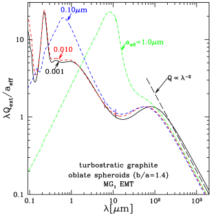
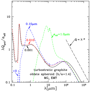
Figure 14: Extinction and polarization cross sections for oblate spheroids with axial ratio $b/a=1.4$. For $a=0.1\micron$, $Q_{\rm pol}<0$ for $\lambda<0.25\micron$; $\lambda|Q_{\rm pol}|/a_{\rm eff}$ is shown. Tabulated cross sections are available at http://www.astro.princeton.edu/$\sim$draine/dust/D16graphite/D16graphite.html and http://arks.princeton.edu/ark:/88435/dsp01nc580q118 .

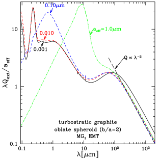
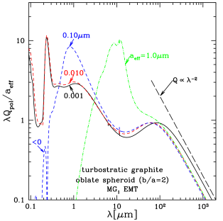
Figure 15: Extinction and polarization cross sections for oblate spheroids with axial ratio $b/a=2$. For $a=0.1\micron$, $Q_{\rm pol}<0$ for $\lambda<0.25\micron$; $\lambda|Q_{\rm pol}|/a_{\rm eff}$ is shown. Tabulated cross sections are available at http://www.astro.princeton.edu/$\sim$draine/dust/D16graphite/D16graphite.html and http://arks.princeton.edu/ark:/88435/dsp01nc580q118 .

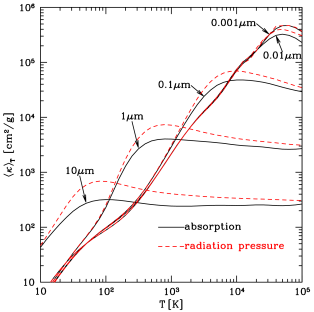
Figure 16: Planck-averaged opacities for absorption and radiation pressure for turbostratic graphite spheres, using the Maxwell Garnett EMT. Planck-averaged opacities for these and other sizes are available at http://www.astro.princeton.edu/$\sim$draine/dust/D16graphite/D16graphite.html and http://arks.princeton.edu/ark:/88435/dsp01nc580q118 .

We have also calculated Planck-averaged cross sections for selected grain sizes, and temperatures from $10\,{\rm K}$ to $10^{5}\,{\rm K}$. Figure 16 shows Planck-averaged opacities for absorption and for radiation pressure:

$$\langle\kappa_{\rm abs}\rangle_{T} \equiv \frac{3}{4\rho a}\frac{\int Q_{\rm abs}(\lambda)B_{\lambda}(T)d\lambda}{\int B_{\lambda}(T)d\lambda}$$ (34)

$$\langle\kappa_{\rm pr}\rangle_{T} \equiv \frac{3}{4\rho a}\frac{\int\left[Q_{\rm abs}(\lambda)+(1-\langle\cos\theta\rangle)Q_{\rm sca})\right]B_{\lambda}(T)d\lambda}{\int B_{\lambda}(T)d\lambda}~{}~{}~{}.$$ (35)

8 Lattice Resonances

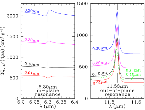
Figure 17: Extinction opacity for randomly-oriented graphite spheres in the neighborhood of the lattice resonances in graphite. The $6.30\micron$ in-plane resonance is probably too weak to be observed. The $11.5\micron$ out-of-plane resonance is an extinction peak, with $\Delta\kappa\approx 640\,{\rm cm}^{2}\,{\rm g}^{-1}$ for single-crystal spheres; turbostratic graphite grains modeled with the Maxwell Garnett EMT (green dashed curve) have $\Delta\kappa\approx 470\,{\rm cm}^{2}\,{\rm g}^{-1}$ and ${\rm FWHM}\approx 0.014\micron$

Draine (1984) noted that if graphite is present in the ISM, the two optically-active lattice resonances, at 6.30 and $11.5\micron$, could conceivably be detected in the interstellar extinction. Here we reexamine this using the dielectric function developed in this paper. An expanded view of the extinction opacity in the neighborhood of the resonances is shown in Figure 17. The $6.30\micron$ in-plane feature is quite weak, and changes from being an extinction minimum for small grains, to a complicated profile for $a\gtrsim 0.1\micron$ grains where scattering is no longer negligible. After averaging over a size distribution, the prospects for detecting the $6.30\micron$ feature do not seem favorable. Observability of the feature is further complicated by the presence of an interstellar absorption feature at $6.2\micron$ that is likely due to similar C-C stretching modes in aromatic hydrocarbons (Schutte et al. 1998; Chiar et al. 2013).

The $11.53\micron$ out-of-plane feature, on the other hand, is more prominent as an extinction excess, and the profile is relatively stable across the range of grain sizes expected in the ISM.

The profiles in Figure 17 were computed using resonance parameters measured for HOPG at room temperature. For randomly-oriented single-crystal grains, the out-of-plane feature peaks at $11.53\micron$, with profile strength $\Delta\kappa\approx 640\,{\rm cm}^{2}\,{\rm g}^{-1}$ and ${\rm FWHM}=0.013\micron$. The feature is relatively narrow, with $\lambda/{\rm FWHM}\approx 870$. If the grains are turbostratic graphite modeled using the Maxwell Garnett effective dielectric function (Eq. 30), the profile is somewhat weaker, with $\Delta\kappa\approx 470\,{\rm cm}^{2}\,{\rm g}^{-1}$ (see Figure 17).

Lab studies and ab-initio modeling of the temperature dependence of the in-plane resonance (Giura et al. 2012) predict a small frequency shift $\delta\omega/\omega\approx 0.0025$ as $T$ is reduced from $T=293\,{\rm K}$ to $T\approx 20\,{\rm K}$ (appropriate for interstellar grains). There do not appear to be studies of the $T$-dependence of the $11.53\micron$ out-of-plane mode, but if the fractional frequency shift is similar, the $11.53\micron$ peak might shift to $\sim$$11.50\micron$.

If a fraction $f_{\rm C,gra}$ of interstellar carbon is in graphite, then we expect the resonance feature to have a maximum optical depth

$$\Delta\tau_{11.5}=8.3\times 10^{-25}\left(\frac{f_{\rm C,gra}}{0.3}\right)\,{\rm cm}^{2}N_{\rm H}$$ (36)

By contrast, the broad silicate feature has $\Delta\tau_{9.7}=2.7\times 10^{-23}\,{\rm cm}^{2}N_{\rm H}$ (Roche & Aitken 1984). Thus, the peak optical depth of the graphite feature would be

$$\Delta\tau_{11.5}=0.031\left(\frac{f_{\rm C,gra}}{0.3}\right)\Delta\tau_{9.7}~{}~{}~{};$$ (37)

the feature is not expected to be very strong. Spectra taken with the Spitzer IRS-LRS with $R\approx 100$ would have diluted this by a factor of $\sim 10$, and the feature would not have been detectable even in high S/N IRS-LRS spectra.

The MIRI spectrograph on JWST, with $R\approx 2500$ near $11.5\micron$, will be well-suited for study of this feature. If the resonance parameters for HOPG apply to interestellar graphite, MIRI may be able to detect interstellar graphite, or obtain useful upper limits on its abundance, from high S/N spectra of stars seen through extinction with $\Delta\tau_{9.7}\gtrsim 1$.

9 X-Ray Absorption and Scattering by Graphite Grains

9.1 Randomly-Oriented Grains

X-ray absorption and scattering by carbonaceous dust near the C K edge can be important on moderately-reddened sightlines. Figure 18 shows the extinction and scattering opacities for randomly-oriented graphite spheres with three selected radii, and also averaged over two size distributions: (1) the “MRN” size distribution, $dn/da\propto a^{-3.5}$ for $0.005\micron<a<0.25\micron$ from Mathis et al. (1977), and (2) the size distribution for carbonaceous grains from Weingartner & Draine (2001).

The cross sections for X-ray scattering and absorption were calculated using the $\nicefrac{{1}}{{3}}$ - $\nicefrac{{2}}{{3}}$ approximation and the Mie theory code of Wiscombe (1980). Because the dielectric function is close to unity, we expect the $\nicefrac{{1}}{{3}}$ - $\nicefrac{{2}}{{3}}$ approximation to be accurate at X-ray energies, even in the present application, where the grain radii $a\approx 0.1\micron$ are large compared to the wavelength $\lambda\approx 0.004\micron$.

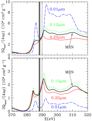
Figure 18: Extinction and scattering opacities for randomly-oriented graphite spheres. Broken curves: selected sizes. Solid curves: MRN distribution, $dn/da\propto a^{-3.5}$, for $0.005\micron<a<0.25\micron$. Vertical lines: positions of strong $1s^{2}2s^{2}2p\rightarrow 1s2s^{2}2p^{2}$ absorption lines of C II (see text).

If $A_{V}/{\rm mag}=5.34(N_{\rm H}/10^{22}\,{\rm cm}^{-2})$, then the graphite grains contribute a mass surface density $\Sigma_{\rm C,gra}=3.73\times 10^{-6}(f_{\rm C,gra}/0.3)(A_{V}/{\rm mag})\,{\rm g}\,{\rm cm}^{-2}$.

With $\kappa_{\rm ext}(292\,{\rm eV})\approx 4\times 10^{4}\,{\rm cm}^{2}\,{\rm g}^{-1}$ for the MRN size distribution, this gives an optical depth

$$\tau_{\rm ext}(292\,{\rm eV})\approx 0.15\left(\frac{f_{\rm C,gra}}{0.3}\right)A_{V}~{}~{}~{},$$ (38)

thus X-ray spectroscopy with moderate signal-to-noise and energy resolution of a few eV would be able to detect the broad extinction feature due to the K shell on sightlines with $A_{V}\gtrsim 1$. The extinction should peak at $\sim 292\,{\rm eV}$; with energy resolution of $\sim 2\,{\rm eV}$, this peak can be separated from the three C II $1s\!\rightarrow\!2p$ absorption lines (see below). Unfortunately, the graphite absorption features which are sharp for small ($\sim 0.01\micron$) grains are suppressed by internal absorption in the larger grains that dominate the mass in the MRN distribution, and the resulting spectroscopic signature is not very pronounced.

For the MRN distribution, about 40% of the extinction near the K edge comes from scattering. Spectroscopy of the scattering halo would show an intensity maximum at $\sim 291\,{\rm eV}$, and a secondary maximum at $\sim 284\,{\rm eV}$.

In the diffuse ISM, most of the gas-phase carbon is singly-ionized. Ground state C II has strong $1s^{2}2s^{2}2p\,{\rm{}^{2}P}^{o}\rightarrow 1s2s^{2}2p^{2}({\rm{}^{2}D},{\rm{}^{2}P},{\rm{}^{2}S})$ absorption lines at $E=287.9\,{\rm eV}$, $288.4\,{\rm eV}$, and $289.9\,{\rm eV}$ (Jannitti et al. 1993; Schlachter et al. 2004), with oscillator strengths $f=0.102$, $0.193$, and $0.0197$ (Wang & Zhou 2007). The resulting $1s2s^{2}2p^{2}$ excited states (${\rm{}^{2}D},{\rm{}^{2}P},{\rm{}^{2}S}$) generally deexcite via the Auger effect, resulting in relatively large intrinsic linewidth $\Delta E\approx 0.1\,{\rm eV}$. The lines, shown in Figure 18, will appear as strong absorption features near $288\,{\rm eV}$, together with the broader features due to dust.

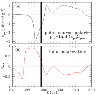
Figure 19: Polarization opacity $\kappa_{\rm pol}$ for single-crystal graphite grains with $a_{\rm eff}=0.1\micron$ and $\hat{\bf c}\perp\hat{\bf k}$. $p>0$ for ${\bf E}\parallel\hat{\bf c}$. The scattered halo polarization $p_{\rm sca}>0$ when ${\bf E}_{\rm sca}\parallel\hat{\bf c}$. Vertical lines: positions of strong K$\alpha$ $1s^{2}2s^{2}2p\rightarrow 1s2s^{2}2p^{2}$ absorption lines of C II (see text).

9.2 Aligned Graphite Grains: Polarized Extinction and Scattering

Suppose that the Galactic magnetic field ${\bf B}_{0}$ is perpendicular to the line-of-sight to an X-ray source, and that a fraction $f_{\rm gra,algn}$ of all of the carbon on the sightline is present in graphite crystals with $\hat{\bf c}\parallel{\bf B}_{0}$; the remaining $1-f_{\rm gra,algn}$ of the C atoms are either not in graphite, or are in randomly-oriented graphite crystals.

If the total carbon abundance is C/H=295ppm, and $N_{\rm H}=1.87\times 10^{21}\,{\rm cm}^{-2}A_{V}/{\rm mag}$, then radiation reaching us from a point source seen through dust with extinction $A_{V}$ will acquire a polarization

$$P_{\rm ps}=\tanh\left[\kappa_{\rm pol}\times 1.12\times 10^{-5}\,{\rm g}\,{\rm cm}^{-2}f_{\rm gra,algn}\left(\frac{A_{V}}{\rm mag}\right)\right]~{}~{}~{}.$$ (39)

With $\kappa_{\rm pol}(285\,{\rm eV})\approx-3\times 10^{4}\,{\rm cm}^{2}\,{\rm g}^{-1}$ (see Fig. 19),

$$P_{\rm ps}(285\,{\rm eV})=\tanh(-0.35f_{\rm gra,algn}A_{V})\approx-0.35f_{\rm gra,aligned}(A_{V}/{\rm mag})~{}~{}~{}.$$ (40)

Thus if, say, 10% of the carbon were in aligned graphite crystals with $\hat{\bf c}\perp$ line-of-sight on a sightline with $A_{V}=1$, the polarization of the point source would be 3.5% at $285\,{\rm eV}$. While the polarization would increase for increased $A_{V}$, the overall attenuation by the ISM makes it difficult to carry out observations near the C K edge on sightlines with $A_{V}\gtrsim 2$.

For oriented graphite grains, the scattered X-rays would show energy-dependent polarization, as in Fig.  19. The X-ray scattered halo could achieve polarizations as large as 85% at $284\,{\rm eV}$, although this would be reduced when the effects of polarized absorption, and unpolarized scattering by nonaligned or nongraphitic grains, are included. Because the polarization is strongly energy-dependent (see Figure 19) an instrument intended to measure it should have $\lesssim 10\,{\rm eV}$ energy resolution.

At this time there are no instruments, existing or planned, that could measure such X-ray polarization. Proposed X-ray polarimetry missions (GEMS and IXPE) are intended to operate only above 2 keV, and have minimal energy resolution.

10 Discussion

The dielectric function of graphite continues to be uncertain, which is surprising for such a well-defined and fundamental material. In particular, there are striking differences in the reported optical constants for ${\bf E}\parallel\hat{\bf c}$ in the 1–5$\,{\rm eV}$ range for, as seen in Figure 2, and there do not appear to be any published measurements between 0.3 and 1$\,{\rm eV}$. The synthetic dielectric functions obtained here represent our best effort to reconcile the published experimental results. We hope that there will be renewed efforts to accurately measure both $\epsilon_{\perp}$ and $\epsilon_{\parallel}$ at wavelengths from the infrared to the ultraviolet.

Of particular interest would be study of the 11.5$\micron$ lattice resonance at temperatures $T\approx 20\,{\rm K}$ appropriate to interstellar grains, to determine the precise wavelength where this resonance should be seen if the interstellar grain population contains a significant amount of graphite. It would also be desirable to study this absorption resonance in disordered forms of carbon that contain microcrystallites of graphite, so that detection of, or upper limits on, the presence of an $11.5\micron$ feature in spectra obtained with MIRI can be used to determine the amount of graphitic carbon in the ISM.

The optical properties of turbostratic graphite at wavelengths $\lambda\gtrsim 10\micron$ remain very uncertain. Different effective medium theories make very different predictions for the effective dielectric function that is intended to characterize turbostratic graphite. Theoretical progress requires obtaining accurate solutions to Maxwell’s equations for particles consisting of turbostratic graphite material. The discrete dipole approximation is one possible numerical technique, but at infrared wavelengths the very large dielectic function for ${\bf E}\perp\hat{\bf c}$ makes DDA calculations numerically challenging. Alternatively, it may be possible to carry out laboratory measurements of absorption by turbostratic graphite particles, to compare with the predictions of different effective medium theories.

11 Summary

The principal results of this paper are as follows:

1. A dielectric tensor for graphite is presented, extending from zero frequency to X-ray energies, and based on laboratory data. Except for the absorption by the K shell electrons at $E>280\,{\rm eV}$, $\epsilon_{\perp}$ and $\epsilon_{\parallel}$ are given by easily-evaluated analytic expressions (Eq. 2 and Tables 2, 3).

2. Techniques for calculating absorption and scattering cross sections are discussed. For single-crystal graphite grains, the simple $\nicefrac{{1}}{{3}}$ - $\nicefrac{{2}}{{3}}$ approximation is exact for $a/\lambda\ll 1$, and is shown to be moderately accurate even when $a/\lambda$ is not small. For $0.1\lesssim\lambda/\micron<0.5$, the $\nicefrac{{1}}{{3}}$ - $\nicefrac{{2}}{{3}}$ approximation gives cross sections that are accurate to within $\pm 5\%$, at least for spheres (see Figure 7. At infrared wavelengths, where $\epsilon_{\perp}$ becomes large, the $\nicefrac{{1}}{{3}}$ - $\nicefrac{{2}}{{3}}$ approximation tends to overestimate $Q_{\rm ext}$ when $a/\lambda\lesssim 0.1$, and to underestimate $Q_{\rm ext}$ when $0.1<a/\lambda\lesssim 0.2$. For $\lambda=10\micron$, the $\nicefrac{{1}}{{3}}$ - $\nicefrac{{2}}{{3}}$ approximation may overestimate $Q_{\rm ext}$ by as much as 40%. If errors of tens of percent are tolerable, the $\nicefrac{{1}}{{3}}$ - $\nicefrac{{2}}{{3}}$ approximation can be used when more exact DDA calculations are unavailable.

3. If a significant fraction of interstellar carbon is in the form of graphite, the $11.5\micron$ lattice resonance may be detectable with $R\gtrsim 10^{3}$ spectroscopy (see Fig. 17). The MIRI spectrograph on JWST will be able to detect or obtain useful upper limits on the 11.5$\micron$ feature.

4. For grains consisting of turbostratic graphite (randomly-oriented graphite microcrystallites), either the Maxwell Garnett or Bruggeman theories can be used to obtain an effective dielectric function for use in scattering calculations at wavelengths $\lambda\lesssim 0.5\micron$. However, at longer wavelengths, the Maxwell Garnett and Bruggeman estimates diverge. We suggest that one of the Maxwell Garnett estimates – MG₁ given by Eq. (30) – may be the best choice for turbostratic graphite particles. However, the applicability of effective medium theory to turbostratic graphite at $\lambda\gtrsim 10\micron$ remains uncertain, and additional theoretical and/or experimental work is required.

5. The carbon K shell absorption in graphite is anisotropic. If interstellar carbon were substantially in small, aligned graphite grains, the K edge absorption would result in significant polarization of the transmitted X-rays between $280$ and $310\,{\rm eV}$. The scattered X-ray halo produced by aligned grains will be oppositely polarized (see Fig. 19). Currently planned X-ray telescopes lack polarimetric capabilities near the carbon K edge, but future X-ray observatories might be able to detect or constrain such polarization.

References

- Abeles & Gittleman (1976) Abeles, B., & Gittleman, J. I. 1976, Appl. Opt., 15, 2328
- Allamandola et al. (1985) Allamandola, L. J., Tielens, A. G. G. M., & Barker, J. R. 1985, ApJ, 290, L25
- Altarelli et al. (1972) Altarelli, M., Dexter, D. L., Nussenzveig, H. M., & Smith, D. Y. 1972, Phys. Rev. B, 6, 4502
- Asplund et al. (2009) Asplund, M., Grevesse, N., Sauval, A. J., & Scott, P. 2009, ARA&A, 47, 481
- Bernatowicz et al. (1996) Bernatowicz, T. J., Cowsik, R., Gibbons, P. C., et al. 1996, ApJ, 472, 760
- Bohren (2010) Bohren, C. F. 2010, European Journal of Physics, 31, 573
- Bohren & Huffman (1983) Bohren, C. F., & Huffman, D. R. 1983, Absorption and Scattering of Light by Small Particles (New York: Wiley)
- Borghesi & Guizzetti (1991) Borghesi, A., & Guizzetti, G. 1991, in Handbook of optical constants of solids II, ed. Palik, E. D. (New York: Academic Press), 449
- Campbell et al. (2015) Campbell, E. K., Holz, M., Gerlich, D., & Maier, J. P. 2015, Nature, 523, 322
- Carter et al. (1965) Carter, J. G., Huebner, R. H., Hamm, R. N., & Birkhoff, R. D. 1965, Phys. Rev, 137, 639
- Cayrel & Schatzman (1954) Cayrel, R., & Schatzman, E. 1954, Annales d’Astrophysique, 17, 555
- Chiar et al. (2013) Chiar, J. E., Tielens, A. G. G. M., Adamson, A. J., & Ricca, A. 2013, ApJ, 770, 78
- Collinge & Draine (2004) Collinge, M. J., & Draine, B. T. 2004, J. Opt. Soc. Am. A, 21, 2023
- Croat et al. (2008) Croat, T. K., Stadermann, F. J., & Bernatowicz, T. J. 2008, Meteoritics and Planetary Science, 43, 1497
- Daniels et al. (1970) Daniels, J., Festenberg, C. v., Raether, H., & Zeppenfeld, K. 1970, Springer Tracts in Modern Physics, 54, 77
- Dartois et al. (2004) Dartois, E., Muñoz Caro, G. M., Deboffle, D., & d’Hendecourt, L. 2004, A&A, 423, L33
- Draine (1984) Draine, B. T. 1984, ApJ, 277, L71
- Draine (1988) Draine, B. T. 1988, ApJ, 333, 848
- Draine (1989) Draine, B. T. 1989, in IAU Symp. 135: Interstellar Dust, ed. L. Allamandola & A. Tielens (Dordrecht: Kluwer), 313
- Draine (2011) Draine, B. T. 2011, Physics of the Interstellar and Intergalactic Medium (Princeton, NJ: Princeton Univ. Press)
- Draine & Flatau (1994) Draine, B. T., & Flatau, P. J. 1994, J. Opt. Soc. Am. A, 11, 1491
- Draine & Lee (1984) Draine, B. T., & Lee, H. M. 1984, ApJ, 285, 89
- Draine & Li (2007) Draine, B. T., & Li, A. 2007, ApJ, 657, 810
- Draine & Malhotra (1993) Draine, B. T., & Malhotra, S. 1993, ApJ, 414, 632
- Duley et al. (1993) Duley, W. W., Jones, A. P., Taylor, S. D., & Williams, D. A. 1993, MNRAS, 260, 415
- Duley et al. (1989) Duley, W. W., Jones, A. P., & Williams, D. A. 1989, MNRAS, 236, 709
- Foing & Ehrenfreund (1994) Foing, B. H., & Ehrenfreund, P. 1994, Nature, 369, 296
- Fomichev & Zhukova (1968) Fomichev, V. A., & Zhukova, I. I. 1968, Optics and Spectroscopy, 24, 147
- Giura et al. (2012) Giura, P., Bonini, N., Creff, G., et al. 2012, Phys. Rev. B, 86, 121404
- Greenaway et al. (1969) Greenaway, D. L., Harbeke, G., Bassani, F., & Tosatti, E. 1969, Physical Review, 178, 1340
- Hagemann et al. (1974) Hagemann, H.-J., Gudat, W., & Kunz, C. 1974, DESY Report, SR-74/7, 1
- Hagemann et al. (1975) Hagemann, H.-J., Gudat, W., & Kunz, C. 1975, J. Opt. Soc. Am., 65, 742
- Han et al. (2007) Han, M. Y., Özyilmaz, B., Zhang, Y., & Kim, P. 2007, Physical Review Letters, 98, 206805
- Hecht (1981) Hecht, J. 1981, ApJ, 246, 794
- Hill et al. (1998) Hill, H. G. M., Jones, A. P., & D’Hendecourt, L. B. 1998, A&A, 336, L41
- Hoyle & Wickramasinghe (1962) Hoyle, F., & Wickramasinghe, N. C. 1962, MNRAS, 124, 417
- Jannitti et al. (1993) Jannitti, E., Gaye, M., Mazzoni, M., Nicolosi, P., & Villoresi, P. 1993, Phys. Rev. A, 47, 4033
- Jellison et al. (2007) Jellison, G. E., Jr., Hunn, J. D., & Lee, H. N. 2007, Phys. Rev. B, 76, 085125
- Jeon & Mahan (2005) Jeon, G. S., & Mahan, G. D. 2005, Phys. Rev. B, 71, 184306
- Joblin et al. (1992) Joblin, C., Leger, A., & Martin, P. 1992, ApJ, 393, L79
- Jones (2012a) Jones, A. P. 2012a, A&A, 545, C2
- Jones (2012b) Jones, A. P. 2012b, A&A, 545, C3
- Jones (2012c) Jones, A. P. 2012c, A&A, 540, A1
- Jones (2012d) Jones, A. P. 2012d, A&A, 540, A2
- Jones (2012e) Jones, A. P. 2012e, A&A, 542, A98
- Jones & D’Hendecourt (2004) Jones, A. P., & D’Hendecourt, L. B. 2004, in Astr. Soc. Pac. Conf. Ser. 309, Astrophysics of Dust, ed. A. N. Witt, G. C. Clayton, & B. T. Draine (San Francisco, CA: ASP), 589
- Jones et al. (2013) Jones, A. P., Fanciullo, L., Köhler, M., et al. 2013, A&A, 558, A62
- Klein (1962) Klein, C. A. 1962, J. Appl. Phys., 33, 3338
- Klucker et al. (1974) Klucker, R., Skibowski, M., & Steinmann, W. 1974, Physica Status Solidi B, 65, 703
- Kreibig (1974) Kreibig, U. 1974, Journal of Physics F Metal Physics, 4, 999
- Kuzmenko et al. (2008) Kuzmenko, A. B., van Heumen, E., Carbone, F., & van der Marel, D. 2008, Physical Review Letters, 100, 117401
- Kwok & Zhang (2011) Kwok, S., & Zhang, Y. 2011, Nature, 479, 80
- Kwok & Zhang (2013) Kwok, S., & Zhang, Y. 2013, ApJ, 771, 5
- Landau et al. (1993) Landau, L. D., Lifshitz, E. M., & Pitaevskii, L. P. 1993, Electrodynamics of Continuous Media (Oxford: Pergamon Press)
- Leger & Puget (1984) Leger, A., & Puget, J. L. 1984, A&A, 137, L5
- Léger et al. (1989) Léger, A., Verstraete, L., d’Hendecourt, L., et al. 1989, in IAU Symposium, Vol. 135, Interstellar Dust, ed. L. J. Allamandola & A. G. G. M. Tielens, 173
- Li & Draine (2001) Li, A., & Draine, B. T. 2001, ApJ, 550, L213
- Li & Draine (2012) Li, A., & Draine, B. T. 2012, ApJ, 760, L35
- Manzardo et al. (2012) Manzardo, M., Cappelluti, E., van Heumen, E., & Kuzmenko, A. B. 2012, Phys. Rev. B, 86, 054302
- Mathis et al. (1977) Mathis, J. S., Rumpl, W., & Nordsieck, K. H. 1977, ApJ, 217, 425
- Maxwell Garnett (1904) Maxwell Garnett, J. C. 1904, Philosophical Transactions of the Royal Society of London Series A, 203, 385
- Mennella et al. (1998) Mennella, V., Brucato, J. R., Colangeli, L., et al. 1998, ApJ, 496, 1058
- Moore (1973) Moore, A. W. 1973, Chemistry and physics of carbon, 11, 69
- Mrozowski (1971) Mrozowski, S. 1971, Carbon, 9, 97
- Nemanich et al. (1977) Nemanich, R. J., Lucovsky, G., & Solin, S. A. 1977, Solid State Communications, 23, 117
- Nieva & Przybilla (2012) Nieva, M.-F., & Przybilla, N. 2012, A&A, 539, A143
- Pacilé et al. (2008) Pacilé, D., Papagno, M., Rodríguez, A. F., et al. 2008, Physical Review Letters, 101, 066806
- Papagno et al. (2009) Papagno, M., Fraile Rodríguez, A., Girit, Ç. Ö., et al. 2009, Chemical Physics Letters, 475, 269
- Papoular (2001) Papoular, R. 2001, A&A, 378, 597
- Papoular et al. (1993) Papoular, R., Breton, J., Gensterblum, G., et al. 1993, A&A, 270, L5
- Papoular & Papoular (2009) Papoular, R. J., & Papoular, R. 2009, MNRAS, 394, 2175
- Papoular & Papoular (2014) Papoular, R. J., & Papoular, R. 2014, MNRAS, 443, 2974
- Partoens & Peeters (2006) Partoens, B., & Peeters, F. M. 2006, Phys. Rev. B, 74, 075404
- Parvathi et al. (2012) Parvathi, V. S., Sofia, U. J., Murthy, J., & Babu, B. R. S. 2012, ApJ, 760, 36
- Pendleton & Allamandola (2002) Pendleton, Y. J., & Allamandola, L. J. 2002, ApJS, 138, 75
- Philipp (1977) Philipp, H. R. 1977, Phys. Rev. B, 16, 2896
- Primak (1956) Primak, W. 1956, Phys. Rev, 103, 544
- Purcell & Pennypacker (1973) Purcell, E. M., & Pennypacker, C. R. 1973, ApJ, 186, 705
- Robertson (1986) Robertson, J. 1986, Advances in Physics, 35, 317
- Roche & Aitken (1984) Roche, P. F., & Aitken, D. K. 1984, MNRAS, 208, 481
- Rosenberg et al. (1986) Rosenberg, R. A., Love, P. J., & Rehn, V. 1986, Phys. Rev. B, 33, 4034
- Salama et al. (1996) Salama, F., Bakes, E. L. O., Allamandola, L. J., & Tielens, A. G. G. M. 1996, ApJ, 458, 621
- Schlachter et al. (2004) Schlachter, A. S., Sant’Anna, M. M., Covington, A. M., et al. 2004, Journal of Physics B Atomic Molecular Physics, 37, L103
- Schutte et al. (1998) Schutte, W. A., van der Hucht, K. A., Whittet, D. C. B., et al. 1998, A&A, 337, 261
- Soule (1958) Soule, D. E. 1958, Phys. Rev, 112, 698
- Stagg & Charalampopoulos (1993) Stagg, B. J., & Charalampopoulos, T. T. 1993, Combustion and Flame, 94, 381
- Stecher (1965) Stecher, T. P. 1965, ApJ, 142, 1683
- Stecher & Donn (1965) Stecher, T. P., & Donn, B. 1965, ApJ, 142, 1681
- Stöhr & Jaeger (1982) Stöhr, J., & Jaeger, R. 1982, Phys. Rev. B, 26, 4111
- Taft & Philipp (1965) Taft, E. A., & Philipp, H. R. 1965, Phys. Rev, 138, 197
- Tielens (2008) Tielens, A. G. G. M. 2008, ARA&A, 46, 289
- Tosatti & Bassani (1970) Tosatti, E., & Bassani, F. 1970, Nuovo Cimento B Serie, 65, 161
- Venghaus (1975) Venghaus, H. 1975, Physica Status Solidi B Basic Research, 71, 609
- Venghaus (1977) Venghaus, H. 1977, Physica Status Solidi B Basic Research, 81, 221
- Voshchinnikov & Farafonov (1993) Voshchinnikov, N. V., & Farafonov, V. G. 1993, Ap&SS, 204, 19
- Walker et al. (2015) Walker, G. A. H., Bohlender, D. A., Maier, J. P., & Campbell, E. K. 2015, ApJ, 812, L8
- Wang & Zhou (2007) Wang, G.-L., & Zhou, X.-X. 2007, Chinese Physics, 16, 2361
- Webster (1992) Webster, A. S. 1992, A&A, 257, 750
- Weingartner & Draine (2001) Weingartner, J. C., & Draine, B. T. 2001, ApJ, 548, 296
- Williamson et al. (1965) Williamson, S. J., Foner, S., & Dresselhaus, M. S. 1965, Phys. Rev, 140, 1429
- Wiscombe (1980) Wiscombe, W. J. 1980, Appl. Opt., 19, 1505
- Yang et al. (2013) Yang, X. J., Glaser, R., Li, A., & Zhong, J. X. 2013, ApJ, 776, 110
- Zinner (2014) Zinner, E. 2014, Presolar Grains, ed. A. M. Davis 181