Very high frequency gravitational waves from magnetars and gamma-ray bursts

Abstract

Extremely powerful astrophysical electromagnetic (EM) systems could be possible sources of high-frequency gravitational waves (HFGWs). Here, based on properties of magnetars and gamma-ray bursts (GRBs), we address “Gamma-HFGWs” (with very high-frequency around $10^{20}$ Hz) caused by ultra-strong EM radiation (in the radiation-dominated phase of GRB fireballs) interacting with super-high magnetar surface magnetic fields ($\sim 10^{11}$ T). By certain parameters of distance and power, the Gamma-HFGWs would have far field energy density $\Omega_{gw}$ around $10^{-6}$, and they would cause perturbed signal EM waves of $\sim 10^{-20}$ W/m² in a proposed HFGW detection system based on the EM response to GWs. Specially, Gamma-HFGWs would possess distinctive envelopes with characteristic shapes depending on the particular structures of surface magnetic fields of magnetars, which could be exclusive features helpful to distinguish them from background noise. Results obtained suggest that magnetars could be involved in possible astrophysical EM sources of GWs in the very high-frequency band, and Gamma-HFGWs could be potential targets for observations in the future.

Keywords:High frequency gravitational waves, source of gravitational waves, magnetar, gamma-ray bursts

I Introduction

LIGO has announced four direct detections of gravitational waves (GWs), in the intermediate frequency band, from the physical situation of GW sources occurring due to black hole mergers (Abbott et al., 2016a, b, 2017a, 2017b). This great discovery may inaugurate the era of GW astronomy, and it will also arouse strong interest in looking for GWs from various types of sources in different frequency bands (low, intermediate, high, and very high-frequency bands). In this article, we focus on the possible generation of very high-frequency GWs (around $10^{20}$ Hz) from super-powerful astrophysical electromagnetic (EM) sources.
Actually, the generation of GWs from EM sources, as well as the interaction between GWs and EM fields, has been studied for a long time. Examples include B-mode polarization in the cosmic microwave background (CMB) caused by very low-frequency primordial (relic) GWs (Zhang et al., 2005; Zhao and Li, 2014; Zhao and Zhang, 2006; Ade et al., 2014; Baskaran et al., 2006; A. G. Polnarev, 2008; Seljak and Zaldarriaga, 1997; Pritchard and Kamionkowski, 2005), GWs generated by high-energy astrophysical plasma interacting with intense EM radiation (Servin and Brodin, 2003), GWs produced by EM waves interacting with background magnetic fields (Gertsenshtein, 1962; Boccaletti et al., 1970; Li et al., 2013), and the EM response to HFGWs which would lead to perturbed signal EM waves (Li et al., 2016a, 2003, 2008, 2009a; Wen et al., 2014a, b; Shi et al., 2006; Li et al., 2009b, 2016b). For such issues, the physical conditions and factors of the EM systems, like their strength, structure and scale, will crucially influence the energy and distribution of the generated GWs and the way the perturbed signal EM waves appear (e.g., in proposed HFGW detectors).
Therefore, some celestial bodies with extraordinary EM environments, such as magnetars (which have ultra-high surface magnetic fields), would act as natural astrophysical laboratories to provide extremely strong EM systems as possible GW sources. Thus, in some possible cases, e.g. a binary system consisting of a magnetar and another celestial body which could emit super-powerful radiation as gamma-ray bursts (GRBs), or a magnetar which emits GRBs itself, the system would be a strong EM source of HFGWs by providing powerful EM waves to interact with ultra-high magnetic fields. In this paper, we address such “Gamma-HFGWs” and their possible characteristic properties.

Specifically, the Gamma-HFGWs would be produced by high-energy radiations of GRBs (up to $10^{53}$ erg or even higher (Piran, 2005)) interacting with the super strong surface magnetic fields of the magnetar ($\sim 10^{11}$ T) (Metzger et al., 2007). However, for conservative calculation, we only consider the contribution of such high-energy radiation within the radiation-dominated phase in the fireball of a GRB, where the energy density of radiation decays quite fast, by $r^{-4}$ (because of the conversion of radiation photons into electron-positron pairs during the transition process into the matter-dominated phase (Piran, 1999)). Based on the Einstein-Maxwell equations (Gertsenshtein, 1962; W. K. De Logi and Mickelson, 1977) in the framework of general relativity, such radiation and surface magnetic fields will provide us with a quickly varying energy-momentum tensor $T^{\mu\nu}$ as a powerful HFGW source. By typical parameters, we estimate that the Gamma-HFGWs (with very high-frequency $\sim 10^{20}$ Hz) would have an energy density $\Omega_{gw}$ around $10^{-6}$ at an observational distance of $\sim Mpc$ away from the source. This level of $\Omega_{gw}$ could cause perturbed signal EM waves of strength $\sim 10^{-20}$ W/m² in a proposed HFGW detector based on the EM response to HFGWs and the synchro-resonance effect (Li et al., 2003, 2016a, 2008, 2009a; Wen et al., 2014a, b; Li et al., 2013).

Only components of magnetic fields which are perpendicular to the direction of propagation of GRB radiation will contribute to the generation of Gamma-HFGWs (Gertsenshtein, 1962; W. K. De Logi and Mickelson, 1977) (this case can be called the “perpendicular condition”). Thus, the angular distributions of Gamma-HFGWs will appear in specific special patterns (e.g. the equator-maximum-pattern or quadrupole-like pattern) according to the specific mode and structure of the surface magnetic fields (their exact structure is still unknown so far, so we here employ a typical possible form (Rädler et al., 2001) as an example for this paper). The misalignment of the rotational axis and magnetic axis of a magnetar would lead to particular pulse-like envelopes of energy density of Gamma-HFGWs in the observational direction. Such unique envelopes would be distinctive properties and criteria to distinguish the signals of Gamma-HFGWs from background noise.

This paper is structured as follows. In Section 2, we present the form used for the super strong surface magnetic field of the magnetar. In Section 3, the generation of Gamma-HFGWs and their energy density are estimated. In Section 4, the characteristic envelopes of Gamma-HFGWs are expressed. In Section 5, we give a summary and conclusions, and present discussion of the consequences of our derivation.

II Model of super strong surface magnetic fields of magnetar

The structure of magnetic fields of magnetar, will delineate a magnetar’s interaction with EM waves. However, so far, we are not sure about the concrete form of surface distribution of such magnetic fields, although it’s well-known that magnetars can have extremely strong surface magnetic fields reaching to $\sim 10^{11}Tesla$ or even higher (Metzger et al., 2007). Thus, in this paper, we take a typical form (Rädler et al., 2001) of magnetic fields of a magnetar as an example and basis for calculations in the later sections, i.e., the surface magnetic fields for a magnetar could be generally expressed as (Rädler et al., 2001):

$$\textbf{B}^{surf}=\vec{\bigtriangledown}\times(\vec{r}\times\vec{\bigtriangledown}S),$$ (1)

Where the symbol $\vec{\bigtriangledown}$ represents the three-dimensional vector differential operator referring to the scale factors $h_{i}$ to describe the geometry of $t=constant$ spacelike hypersurfaces with the line element different to that in a flat spacetime [see details in the Appendix A of ref. (Rädler et al., 2001)]. Here we use the spherical coordinates with the orthonormal basis of $\textbf{e}_{r}$, $\textbf{e}_{\theta}$ and $\textbf{e}_{\phi}$; the $\textbf{r}=r\textbf{e}_{r}$, and the $\textbf{B}=B_{r}\textbf{e}_{r}+B_{\theta}\textbf{e}_{\theta}e+B_{\phi}\textbf{e}_{\phi}$. The scalar function $S$ can be expanded in a series of spherical harmonics:

$$S=S(l,m)=S_{l}^{m}(r)Y_{l}^{m}(\theta,\phi),$$

$$and~{}Y_{l}^{m}(\theta,\phi)=P_{l}^{m}(\cos\theta)e^{im\phi};$$ (2)

where $P_{l}^{m}(\cos\theta)$ is Legendre polynomial. For $l=1,m=0$ (corresponding to the dipole mode), Eq. (II) gives:

$$S(1,0) = C\frac{\cos\theta}{r^{2}}\sum_{\nu=0}^{\infty}a_{\nu}(\frac{2M}{r})^{\nu},$$

$$a_{0} = 1,a_{\nu}=\frac{(1+\nu)^{2}-1}{(3+\nu)\nu}a_{\nu-1},(for~{}\nu\geq 1),$$

Define the metric $h$ as (Rädler et al., 2001):

$$~{}h=h(r)=(1-\frac{2M}{r})^{-\frac{1}{2}},M=\frac{G{m(r)}}{c^{2}},$$ (4)

From Eqs. (1) to (II), magnetic field (the dipole component) can be given,

$$\textbf{B}^{surf}(1,0)=\vec{\bigtriangledown}\times(\vec{r}\times\vec{\bigtriangledown}S(1,0))$$ (5)

$$= C_{1}\cos\theta\frac{1}{r^{3}}\sum_{\nu=0}^{\infty}a_{\nu}(\frac{2M}{r})^{\nu}\vec{e}_{r}$$

$$+ C_{1}\sin\theta\frac{1}{r^{3}h}\sum_{\nu=0}^{\infty}(\nu+1)a_{\nu}(\frac{2M}{r})^{\nu}\vec{e}_{\theta},$$

By calculations of the summation terms in Eq. (5), a typical analytical expression of the surface magnetic field of the magnetar could be written as [see Fig.1(a)]:

$$\textbf{B}^{surf}_{di}(1,0)$$

$$= 2C_{1}\cos\theta\frac{1}{r^{3}}\frac{-3r[r^{2}\log(1-\frac{2M}{r})+2M(M+r)]}{8M^{3}}\vec{e}_{r}$$

$$+ C_{1}\frac{\sin\theta}{r^{3}h}\frac{3r^{2}[2M(\frac{M}{r-2M}+1)+r\log(1-\frac{2M}{r})]}{4M^{3}}\vec{e}_{\theta},$$

In Eq. (4) we have that $m(r)$ is the mass function that determines the total mass enclosed within the sphere of radius $r$, and $m(r)\equiv$ magnetar mass in our case because we only concern magnetic fields outside magnetars. Here, $C_{1}$ and $C_{2}$ (see below) are constants that have been calibrated to typical strengths of surface magnetic fields (e.g. $10^{11}T$).
Similarly, for the case of $l=2$, $m=0$, we have the quadrupole form of surface magnetic fields [Fig.1(b)]:

$$\textbf{B}^{surf}_{quad}(2,0)=3C_{2}(3\cos^{2}\theta-1)\frac{1}{r^{4}}$$

$$\cdot \frac{-3r[r^{2}\log(1-\frac{2M}{r})+2M(M+r)]}{8M^{3}}\vec{e}_{r}$$

$$+ 3C_{2}\cos\theta\sin\theta\frac{1}{r^{4}h}$$

$$\cdot \frac{3r[2M(\frac{4M^{2}}{r-2M}+M+r)+r^{2}\log(1-\frac{2M}{r})]}{8M^{3}}\vec{e}_{\theta},$$

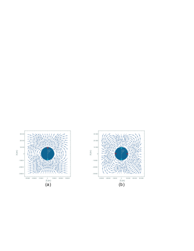
Figure 1: Two-dimensional presentations of models of magnetar surface magnetic fields in dipole and quadrupole modes. Poloidal components of dipole mode (a) and quadrupole mode (b) surface magnetic fields of magnetar reach their maximum at polar angle $\theta=\pi/2$ and $\theta=\pi/4,~{}3\pi/4$ respectively. Patterns of surface magnetic fields will crucially influence the angular distributions of Gamma-HFGWs

For magnetars, the surface magnetic fields in quadrupole mode would have comparable strength to that of dipole mode (Thompson, 2008). In dipole mode, the poloidal components [see $\vec{e}_{\theta}$ component in Eq. (II)] have the maximal values at polar angle $\theta=\pi/2$ [Fig.1(a)], and the radial components [see $\vec{e}_{r}$ component in Eq. (II)] have their maximum around polar angle $\theta=0$ and $\pi$ (two magnetic poles). The $\theta=\pi/2$ means the direction perpendicular to the magnetic axis of a magnetar, and $\theta=0$ means the direction in the magnetic axis. Differently, in quadrupole mode the poloidal components [see $\vec{e}_{\theta}$ component in Eq. (II)] have maximal values around $\theta=\pi/4$ and $3\pi/4$ [Fig.1(b)]. These particular distributions of surface magnetic fields will act key roles to determine the angular distributions of the Gamma-HFGWs generated by EM sources from magnetars (see following sections).

III Gamma-HFGWs from magnetars and GRBs

It is safe to state that the extremely powerful radiations (around $\sim 10^{51}$ to $10^{53}erg$ or even higher in a few seconds) make GRBs the most luminous (electromagnetically) objects in the Universe (Piran, 1999; Kulkarni et al., 1998, 1999). According to general relativity, interactions between such radiation of high energy EM bursts and ultra-intense surface magnetic fields of magnetars ($\sim 10^{11}T$ or higher (Metzger et al., 2007)), can provide a fast varying energy momentum tensor $T^{\mu\nu}$ as a strong EM source of HFGWs in very high-frequency band (denoted as “Gamma-HFGWs”, the same hereafter).
Lots of models of inner engine of GRBs had been proposed to explain the origin of so huge amount of energy, such as black-hole accretion, collapsar model, supernova model (see review by Piran (Piran, 2005)), binary neutron star mergers (Eichler et al., 1999; Narayan et al., 1992), black hole-neutron star mergers (Paczynski, 1991), Blandford-Znajek mechanism (Blandford and Znajek, 1977), pulsar model (Piran, 2005; Usov, 1992, 1994; Smolsky and Usov, 1996, 2000; G. Drenkhahn and H. C. Spruit, 2002; H. C. Spruit et al., 2001), magnetar model (Thompson and Duncan, 2001a; Eichler, 2002; Zhang and Meszaros, 2001; Thompson, 2006), etc. Specially, the magnetar model of GRBs with fireball scenarios are studied by some previous works (Corsi and M sz ros, 2009; Dai, 2004; Pires et al., 2014; Thompson and Gill, 2014; Fargion and Grossi, 2006; DallOsso et al., 2011), and a possible case is to consider fireball trapped near the magnetar surface by the super strong magnetic fields (Thompson and Duncan, 1995, 2001b; Kaneko et al., 2010; Metzger et al., 2008; Ibrahim et al., 2001; Jia et al., 2008; Israel et al., 2008). Therefore, no matter in the case that GRBs source would combine magnetar as a binary system, or in the case that magnetar itself would become the source of GRBs, once such GRB radiations interact with the magnetar surface magnetic fields, it could lead to considerable generation of Gamma-HFGWs.

GRBs have complicated process and mechanism, especially for the problem of inner engine that produces the relativistic energy flow (Piran, 1999). According to fireball internal-external shocks model, the generation of observed GRBs would be on account of the process of kinetic energy of ultra-relativistic flow to dissipate during the internal collisions (internal shocks) (Piran, 2005). Piran had summed (Piran, 1999) generic pictures to suggest that in the fireball model the GRBs are composed of several stages: (i) a compact inner “engine” to produce a relativistic energy flow, (ii) stage of energy transportation, (iii) conversion of this energy to observed prompt radiation, (iv) conversion of the remaining energy to afterglow.
For stage (i), Goodman (Goodman, 1986) and Paczynski (Paczynski, 1986) proposed the relativistic fireball model and had shown that the sudden release of a large quantity of gamma-ray photons into such compact region can lead to an opaque photon-lepton fireball (pairs-radiation plasma, by production of electron-positron pairs from photon-photon scattering) (Piran, 1999), because if the photon energy reaches high enough ($>511KeV$), electron-positron pairs can be formed from the radiations.

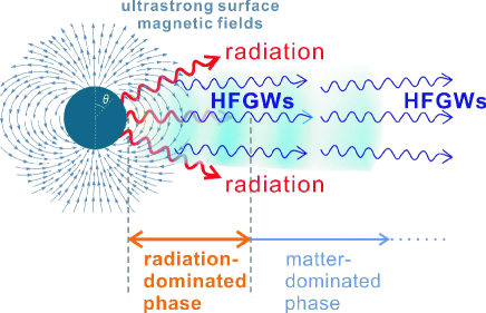
Figure 2: Gamma-HFGWs caused by strong radiations (in radiation-dominated phase of fireball in GRBs) interacting with ultrastrong surface magnetic fields (dipole mode) of magnetar. Expanding fireball has two basic phases: radiation-dominated phase (typically $<10^{7}m$) and matter-dominated phase ($>10^{7}m$); in radiation-dominated stage, energy of strong radiation decays quite quickly by $distance^{-4}$ (Piran, 1999). However, in very early stage of the radiation-dominated phase, photon energy still dominates in the fireball and can provide extremely powerful EM source to interact with the strong surface magnetic fields, i.e. provide a fast varying energy momentum tensor $T^{\mu\nu}$ as a strong EM source of generation of Gamma-HFGWs, and such HFGWs are transparent to the optically-thick fireball. This figure is an intuitive demonstration and the scale is not exact.

Thereafter, pairs-radiation plasma behaves like a perfect fluid and expands by its own pressure (Piran, 1999). During this expansion and energy transportation stage, the expanding fireball has two basic phases (Piran, 1999): a radiation-dominated phase and a matter-dominated phase (see Fig.2). In early stage of radiation-dominated phase, most energy comes out as high-energy radiation (Piran et al., 1993), and the fluid of plasma accelerates in the process of expansion with very large Lorentz factors, and then a transition from the radiation-dominated phase to the matter-dominated phase takes place when the fireball has a size about $10^{7}m$ (typical value) (Piran, 1999). Crucially, in the radiation-dominated stage, energy of radiation decays by $distance^{-4}$ (much faster than normal spherical radiation in free space which decays by $distance^{-2}$, due to the formation of electron-positron pairs from photons, see details in sec.6.3 of ref. (Piran, 1999)).
Therefore, although GRBs have overall extremely complex evolutionary histories, in the early stage of the radiation-dominated phase, the photon energy still dominates in the fireball and we have that photon energy can interact with extremely strong magnetar surface magnetic fields in order to become a considerable EM source of Gamma-HFGWs (Fig.2). While, for conservative estimation procedures used here we will consider only a much shorter interaction range for calculation (of generation of Gamma-HFGWs) as occurring in the very early stage of the radiation-dominate phase, i.e., we are only considering the interaction range from $10^{4}m$ (supposed magnetar radius) to $2\times 10^{4}m$.

In local area we have that, for a specific propagation direction (i.e. z-direction), the energy flux density of this strong EM source of Gamma-HFGWs can be represented by the “0-3” component of an energy momentum tensor $\mathop{T^{03}}\limits^{(1)}$ (Landau and Lifshitz, 1975; Li et al., 2008):

$$\mathop{T^{03}}\limits^{(1)}=\frac{-1}{\mu_{0}}(F^{0(0)}_{~{}\alpha}\tilde{F}^{3\alpha(1)}+\tilde{F}^{0(1)}_{~{}\alpha}{F}^{3\alpha(0)})$$ (8)

$$= \frac{-1}{\mu_{0}}[0+\tilde{F}^{0(1)}_{~{}1}F^{31(0)}]$$

$$= \frac{1}{\mu_{0}c}\tilde{E}^{(1)burst}_{x}e^{i(kz-\omega t)}B^{(0)surf}_{\theta},$$

Here, “$k$” and $\tilde{F}^{\mu\nu(1)}$ are wave vector and EM tensor of EM waves of GRBs; $F^{\mu\nu(0)}$ is an EM tensor of the surface magnetic fields. Here we define the outward radial direction as the z-direction, i.e., $F^{31(0)}=-F^{13(0)}=-B^{(0)surf}_{y}=B^{(0)surf}_{\theta}=10^{11}T$ (simply treat other components as zero, because only the $B^{(0)surf}_{\theta}$ [poloidal component of the surface magnetic fields. I.e. the $\vec{e}_{\theta}$ components in Eqs. (II) and (II)] which is perpendicular to the direction of GRBs in supposed given configuration here, will contribute to the generation of HFGWs (Gertsenshtein, 1962; W. K. De Logi and Mickelson, 1977) (noted as “perpendicular condition”, the same hereafter). Thus, through magnetar surface magnetic fields in dipole-mode, generated HFGWs will follow an equator-maximum-pattern, i.e., their angular distribution mainly concentrate around the region of polar angle $\theta=\pi/2$ (equator area). What is noticeable is that magnetar surface magnetic fields in quadrupole-mode, generate Gamma-HFGWs which would also radiate in a quadrupole pattern concentrating around $\theta=\pi/4$ and $3\pi/4$.
For estimating such Gamma-HFGWs, we can first focus on a very thin layer in local area, with the assumption that the radiation and surface magnetic fields can be treated as being uniform. So the generation of Gamma-HFGWs can be expected to be given by the linearized Einstein field equation as follows:

$$\Box\tilde{h}^{\mu\nu}(z,t)=-\frac{16\pi G}{c^{4}}T^{\mu\nu}$$ (9)

$$= -\frac{16\pi G}{c^{4}}\cdot\frac{1}{\mu_{0}c}\tilde{E}^{(1)burst}_{x}e^{i(kz-\omega_{\gamma}t)}B^{(0)surf}_{\theta},$$

A solution of the above linearized Einstein equation can be obtained to be presented as:

$$\tilde{h}^{\mu\nu}(z,t)=A^{\gamma}e^{i(kz-\omega t+\frac{3\pi}{2})}$$ (10)

$$= \frac{-z8\pi G\tilde{E}^{(1)burst}_{x}B^{(0)surf}_{\theta}}{kc^{5}\mu_{0}}e^{i(kz-\omega_{\gamma}t+\frac{3\pi}{2})},$$

This local solution composed of planar GWs caused by a uniform EM source clearly shows that the accumulation effect (because the HFGWs caused by radiation will be accumulated during their propagation along with the radiation synchronously due to their identical speed of light) is proportion to the accumulative distance (term “$z$”), which is in total accordance to our previous results derived by use of the accumulation effect which is the case of what happens when we use planar GWs (Boccaletti et al., 1970).
However, for our case, using the Gamma-HFGWs, the situation is much more complicated. The background magnetic fields (surface magnetic fields of the magnetar) will nonlinearly decrease along the radial direction [Eq. (II) and Eq. (II)], and the radiation will also decay in the ratio of $\sim 1/z^{4}$ in the radiation-dominated phase (within distance $<10^{7}m$) (Piran, 1999). Thus we find that the compositive contribution of processes due to the generation of Gamma-HFGWs is very different to what happens in the scenario of GW generation (Gertsenshtein, 1962) due to the interaction effects of planar EM waves with uniform magnetic fields. E.g., for a certain power produced by GRB inner engine (noted as $P_{total}^{\gamma}$), we find that the energy flux density of the EM waves at distance of $r_{0}$ (radius of magnetar) should be $P_{total}^{\gamma}/4\pi r_{0}^{2}\sim(\tilde{E}^{(1)burst}_{x.r_{0}})^{2}/(\mu_{0}c)$. Thus, at distance of $r$, electric component of the radiation is $\tilde{E}^{(1)burst}_{x}=\tilde{E}^{(1)burst}_{x.r_{0}}\cdot r_{0}^{2}/r^{2}$.
Therefore, in order to obtain expression of accumulated amplitude of the Gamma-HFGWs ($A^{\gamma}_{accum}$), we can integrate the Gamma-HFGWs generated within very thin local layers [at distance of “r”, with thickness of $dr$, so we can employ the result of Eq. (10)] from the magnetar surface to a certain larger distance “$z$”. If we employ the dipole surface magnetic field [$B^{(0)surf}_{\theta}$, from the second part of Eq. (II), i.e. only take the $\vec{e}_{\theta}$ component, because the $\vec{e}_{r}$ component does not contribute], it can be worked out to read as:

$$A^{\gamma}_{accum}(z)=\int^{z}_{r_{0}}\frac{8\pi G}{{kc}^{5}{\mu_{0}}}(\tilde{E}^{(1)burst}_{x.r_{0}}\cdot\frac{r_{0}^{2}}{r^{2}})B^{(0)surf}_{\theta}\cdot\frac{r}{z}dr$$ (11)

$$= \frac{3C_{1}r_{0}^{2}\tilde{E}^{(1)burst}_{x.r_{0}}\frac{8\pi G}{{kc}^{5}{\mu_{0}}}}{4hM^{3}z}\sin\theta$$

$$\cdot \int^{z}_{r_{0}}\frac{r^{2}[2M\left(\frac{M}{r-2M}+1\right)+rln\left(1-\frac{2M}{r}\right)]}{r^{4}}\,dr$$

$$= \frac{3C_{1}r_{0}^{2}}{z8M^{3}h}\cdot\frac{8\pi G}{{kc}^{5}{\mu_{0}}}\tilde{E}^{(1)burst}_{x.r_{0}}\sin\theta$$

$$\cdot [-\frac{2M}{z}+ln(1-\frac{2M}{z})+2\text{Li}_{2}\frac{2M}{z}$$

$$+ ln\frac{r_{0}}{r_{0}-2M}-2\text{Li}_{2}\frac{2M}{r_{0}}+\frac{2M}{r_{0}}];$$

here, $Li_{2}(\frac{2M}{r_{0}})=\sum_{k=1}^{\infty}\frac{({2M}/{r_{0}})^{k}}{k^{2}}$ is polylogarithm function of order 2 with argument $\frac{2M}{r_{0}}$ (similarly hereafter). The amplitude of GW from any layer at distance of $r$, will decay into level $\propto\cfrac{r}{z}$ (in the ratio of a spherical wave) once the GW propagates to the concerned distance $z$, and this is why we have the term “$\cfrac{r}{z}$” to the left of “$dr$” in the first line of Eq. (11). The Eq. (11) looks complicated, but actually if we take only the first order of $Li_{2}(\frac{2M}{z})$ (i.e., $\frac{2M}{z}$), so that it has a simple asymptotic behavior in large distance:

$$A^{\gamma}_{accum}(z)\rightarrow p1\cdot z^{-1}+p2\cdot z^{-2}$$ (12)

where

$$p1=\frac{3C_{1}r_{0}^{2}}{M^{3}h}\cdot\frac{\pi G}{{kc}^{5}{\mu_{0}}}\tilde{E}^{(1)burst}_{x.r_{0}}\sin\theta$$

$$\cdot(ln\frac{r_{0}}{r_{0}-2M}-2\text{Li}_{2}\frac{2M}{r_{0}}+\frac{2M}{r_{0}}).$$

$$p2=\frac{3C_{1}r_{0}^{2}}{4M^{2}h}\cdot\frac{8\pi G}{{kc}^{5}{\mu_{0}}}\tilde{E}^{(1)burst}_{x.r_{0}}\sin\theta;$$ (13)

Similarly, for when we derive the surface magnetic fields in a quadrupole mode [$B^{(0)surf}_{\theta-quad}$, from the second part of Eq. (II)], we find that the accumulated amplitude of Gamma-HFGWs can be given as:

$$A^{\gamma-quad}_{accum}(z)=\int^{z}_{r_{0}}\frac{8\pi G}{{kc}^{5}{\mu_{0}}}(\tilde{E}^{(1)burst}_{x.r_{0}}\cdot\frac{r_{0}^{2}}{r^{2}})B^{(0)surf}_{\theta-quad}\cdot\frac{r}{z}dr$$ (14)

$$= \frac{9\pi G{C_{2}}\sin\theta\cos\theta\tilde{E}^{(1)burst}_{x.r_{0}}r_{0}^{2}}{kc^{5}\mu_{0}hM^{3}z}\{\frac{-2}{r_{0}}+\frac{2M^{2}}{3}(\frac{-1}{r_{0}^{3}}+\frac{1}{z^{3}})$$

$$+ \frac{2}{z}+\frac{ln(1-2M/r_{0})}{r_{0}}-\frac{ln(1-2M/z)}{z}$$

$$+ [ln\frac{r_{0}}{r_{0}-2M}+ln(1-\frac{2M}{z})]/M\}.$$

So far, it appears that lots of confirmed magnetars are in the Milky Way and can have short distance values of $\sim kpc$, but all currently observed GRBs are from distant galaxies outside the Milky Way, and that the nearest one is GRB 980425 with a redshift $z=0.0085$ or about 36 Mpc away. Even if any GRB happens within a distance of $\sim kpc$, it would cause globally ozone depletion and it might lead to great ecological damage and extinction of life on Earth (this had been believed as a possible reason of the late Ordovician mass extinction (Thomas et al., 2005)). Therefore, as presented in Table 1, if some magnetars in proper distance with GRBs of suitable power, they still could provide far field effect of Gamma-HFGWs on the Earth (or far field observation points) and meanwhile the power of Gamma-ray can decay into a safe level.
E.g., if the maximum of surface magnetic fields of magnetar $\sim 10^{11}Tesla$, $P_{total}^{\gamma}\sim 10^{54}erg\cdot s^{-1}$, magnetar distance $\sim 1~{}Mpc$, then the energy density $\Omega_{gw}$ of Gamma-HFGW at the Earth could be $\sim 10^{-6}$ [here, $\Omega_{gw}=\frac{\pi^{2}}{3}h^{2}(\nu/\nu_{H})^{2}$, where $\nu_{H}$ is present Hubble frequency, we have that the value of $h$ is given to be the GW amplitude]. Meanwhile, in this case, the power of GRB around the globe is only about $30~{}Watt\cdot m^{-2}$ which is in a safe level far less than the order of magnitude to cause global ozone depletion (Thomas et al., 2005). Other possible cases with suitable parameters of distance and GRB power are also shown in the shaded cells in Table 1. We can find that, $\Omega_{gw}$ in cells with larger distance than these shaded cells, will have too low energy density for potential detection (e.g. in proposed HFGW detectors (Li et al., 2003, 2008, 2016a, 2009a, 2013)), and cells with shorter distance than these shaded cells can have higher $\Omega_{gw}$ but will lead to stronger GRB power which would be dangerous to life and existing ecological systems on Earth. Therefore, the shaded cells in Table 1 present optimal range of Gamma-HFGW sources with proper distance and suitable power (in safe level near globe) to be potentially observational targets of HFGWs from the Earth. Nevertheless, for other cases which cannot provide sizable far field effect on the Earth, such as more faraway GRBs, the possibility still would not be excluded that in the future some spacecraft-based HFGW detector approaching closer area to such sources or some Earth-based detector with greatly enhanced sensitivity would also might be able to capture these Gamma-HFGWs.
Some proposed HFGW detection system (Li et al., 2003, 2008, 2016a, 2009a, 2013) is especially sensitive to GWs in very high-frequency bands. E.g., the Gamma-HFGWs ($\Omega_{gw}\sim 10^{-6}$) would generate the first-order perturbed signal EM waves having power of $\sim 10^{-20}Watt$ per $m^{2}$ in such planned detection system. However, issues about how to experimentally extract and distinguish such perturbed EM signals and relevant techniques, are not key points in this paper, and related topics will be addressed in other works.

Table 1: For some parameters in possible range (not limit to that have already been confirmed by current observations), we estimate accumulated energy density ($\Omega_{gw}$, at far observational distance) of the Gamma-HFGWs generated by interaction between powerful radiation of GRBs and ultra-high surface magnetic fields of magnetars. Representative frequency of Gamma-ray (also of the Gamma-HFGWs) is set to $\sim 10^{20}Hz$. Shaded cells in the table indicate the parameter range where the Gamma-HFGWs would cause perturbed signal EM waves of $\sim 10^{-20}W/m^{2}$ in proposed HFGW detector meanwhile corresponding power of GRBs would decay into about $30~{}Watt/m^{2}$ (which is safe, since it is far less than the power able to cause globally ozone depletion and to result in extinction of lives). Therefore, the shaded cells represent the Gamma-HFGW sources with optimal parameters to be possible potential observational targets in the future.

Observational Dipole mode, $B^{surf}=4\times 10^{11}T$, distance away $P_{total}^{\gamma}$ ($erg\cdot s^{-1}$) from magnetar $3\times 10^{54}$ $3\times 10^{52}$ $3\times 10^{50}$ $\sim~{}10kpc$ $\Omega_{gw}^{\gamma}:$  $1.2\times 10^{-2}$  $1.2\times 10^{-4}$  $1.2\times 10^{-6}$ $\sim~{}100kpc$ $\Omega_{gw}^{\gamma}:$  $1.2\times 10^{-4}$  $1.2\times 10^{-6}$  $1.2\times 10^{-8}$ $\sim~{}Mpc$ $\Omega_{gw}^{\gamma}:$ $1.2\times 10^{-6}$  $1.2\times 10^{-8}$  $1.2\times 10^{-10}$ $\sim~{}10Mpc$ $\Omega_{gw}^{\gamma}:$ $1.2\times 10^{-8}$  $1.2\times 10^{-10}$  $1.2\times 10^{-12}$ $\sim~{}Gpc$ $\Omega_{gw}^{\gamma}:$ $1.2\times 10^{-12}$  $1.2\times 10^{-14}$  $1.2\times 10^{-16}$

IV Characteristic envelopes of Gamma-HFGWs

Special geometrical information of structure of magnetar surface magnetic fields, could lead to the existence of characteristic envelopes of energy density of Gamma-HFGWs at specific observation directions, and each special feature of these GW signals can be very helpful in order to distinguish them from background noise signals.

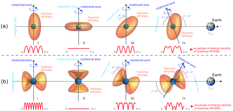
Figure 3: Different angular configurations would cause characteristic envelopes of Gamma-HFGWs. This diagram intuitively explains how various distinctive Gamma-HFGW envelopes received at the Earth (or at far field observation point) can be formed according to different angular sets (angle $\beta$ between rotational and magnetic axis, and angle $\xi$ between rotational axis and observational direction). The energy of Gamma-HFGWs facing the Earth will fluctuate with respect to the rotational phase, and then lead to diverse envelopes of the energy density of Gamma-HFGWs, similar to the formation of pulsing signals from pulsars. Sub-figures (a) and (b) show examples of distinctive envelopes by different $\beta$ and $\xi$, of equator-maximum pattern and quadrupole pattern Gamma-HFGWs (see Eqs. IV and IV). Here $\xi$ is $90^{\circ}$ in cases i-iii, and $\beta$ is $90^{\circ}$, $0^{\circ}$, $45^{\circ}$ and $60^{\circ}$ for cases i to iv, respectively. For some angular sets, the envelopes could be more complicated, e.g. in case iv they appear in unusual distinctive shapes containing both higher and lower mixed peaks.

However, the exact structure of magnetar surface magnetic fields still is unclear so far. Nevertheless, here, as mentioned above, we can take the form of magnetar magnetic fields (Rädler et al., 2001) as an example, to present how particular surface magnetic fields lead to corresponding special GW envelopes. In detailed analysis due to using the fact that the rotational axis and magnetic axis of a given magnetar are usually not identical, we find that during one period, that the maximums of Gamma-HFGWs will not always directly point to the observation direction. Therefore, the envelopes of energy density of these Gamma-HFGWs will thereby vary and fluctuate periodically according to the rotation of magnetar. This phenomenon is similar to the mechanism of what is seen during the analysis of pulsing signals from pulsars (where the misalignment between these two axis of pulsars usually causes the peak of EM radiations facing to the Earth once for every spin period).

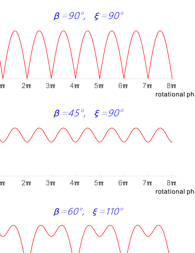
Figure 4: Examples of energy density envelopes of Gamma-HFGWs at the Earth or far field observation points. Typical envelopes of energy density of Gamma-HFGW s are estimated for both equator-maximum case (sub-figure (a) to (d), see Eq. IV) and quadrupole case (sub-figure (e) to (h), see Eq. IV) at various angles $\beta$ and $\xi$ (the same as those defined in Fig. 3). Parameters for the equator-maximum case are: observation distance $=1Mpc$, $P_{total}^{\gamma}=3\times 10^{54}$ erg/s, $Bsurf=4\times 10^{11}T$. Parameters for the quadrupole case are: $P_{total}^{\gamma}=6\times 10^{54}$ erg/s, $B^{surf}=5\times 10^{11}T$. These particular envelopes would be helpful to distinguish the Gamma-HFGWs from background noise in possible detection schemes.

In Fig.3, we present that in different values of angles (i.e. angle between magnetic and rotational axis, noted as $\beta$, and angle between rotational axis and observation direction, noted as $\xi$), envelopes of energy density of Gamma-HFGWs would particularly appear in some pulse-like patterns with various distinctive shapes. By using $\Omega_{gw}=\frac{\pi^{2}}{3}h^{2}(\nu/\nu_{H})^{2}$ and if we evaluate Eqs. (11) to (14), with coordinate transformations, we can have resulting analytical expressions of envelopes of energy density of Gamma-HFGWs at the Earth or far field observation points (here $\Omega_{gw}^{\gamma-eq}$ and $\Omega_{gw}^{\gamma-quad}$ are for equator-maximum and qudrupole cases respectively):

$$\Omega_{gw}^{\gamma-eq}=\frac{\pi^{2}}{3}(A^{\gamma}_{accum}|_{\theta=\pi/2})^{2}(\frac{\nu}{\nu_{H}})^{2}$$

$$\cdot [(\sin\xi\cos\beta\cos\varphi+\cos\xi\sin\beta)^{2}+\sin^{2}\xi\sin^{2}\varphi],$$

and for the quadrupole case,

$$\Omega_{gw}^{\gamma-quad}=\frac{\pi^{2}}{3}(A^{\gamma-quad}_{accum}|_{\theta=\pi/4})^{2}(\frac{\nu}{\nu_{H}})^{2}$$

$$\cdot (\cos\xi\cos{\beta}-\sin\xi\sin{\beta}\cos\varphi)^{2}$$

$$\cdot [(\sin\xi\cos{\beta}\cos\varphi+\cos\xi\sin{\beta})^{2}+\sin^{2}\xi\sin^{2}\varphi].$$

Table 2: Given different effective accumulation distance D of Gamma-HFGWs sources, decay parameter $\Lambda$ of effective radiation in GRBs, decay parameter $\Xi$ of effective strong background magnetic fields, estimated energy density of effective-Gamma-HFGWs ($\Omega^{\gamma-eff}_{gw}$) in far field regions are given. Here $P_{total}^{\gamma}$ is assumed $5\times 10^{54}erg/s$, and far field observational distance sets to $3.3Mpc$ from the magnetar.

effective accumulation		far field (3.3Mpc) $\Omega^{\gamma-eff}_{gw}$ by different decaying parameters $\Lambda$ and $\Xi$
distance around source		$\Lambda=2$, $\Xi=1$;	$\Lambda=2$, $\Xi=2$;	$\Lambda=2$, $\Xi=3$;	$\Lambda=2$, $\Xi=4$;	$\Lambda=4$, $\Xi=5$
$D=10~{}km$	$\Omega^{\gamma-eff}_{gw}:$	$5.3\times 10^{-6}$	$3.0\times 10^{-6}$	$1.8\times 10^{-6}$	$1.1\times 10^{-6}$	$4.3\times 10^{-7}$
$D=100~{}km$	$\Omega^{\gamma-eff}_{gw}:$	$1.7\times 10^{-5}$	$5.2\times 10^{-6}$	$2.3\times 10^{-6}$	$1.3\times 10^{-6}$	$4.3\times 10^{-7}$

For different values of $\beta$ and $\xi$, $\Omega_{gw}$ of Gamma-HFGWs have various distinctive envelopes with respect to rotational phase $\varphi$ (Fig.3), but unlike the pulsars, above envelopes will usually (but not always) come with two peaks during every rotational period [for dipole-mode surface magnetic fields, see Fig.3(a), i.e. the frequency of pulses is double with respect to the rotational frequency], or usually with four peaks for every rotational period [for case with quadrupole-mode surface magnetic fields, see Fig.3(b)], due to special angular distributions of Gamma-HFGWs (see Fig.3). Based on Eqs. (IV) and (IV), typical curves of $\Omega_{gw}$ envelopes of Gamma-HFGWs can be estimated [see Fig.4(1)-(4) for equator-maximum case and (5)-(8) for quadrupole case]. The characteristic envelopes would be helpful to distinguish the Gamma-HFGWs out of background noise, no matter for the model of magnetar magnetic fields we take here, or for other models with different structures.

Given that the mechanism of GRBs is actually quite complex, more detailed issues of generation of HFGWs based on fireball model or other models such as Poynting flux model (Usov, 1992, 1994; Smolsky and Usov, 1996, 2000; G. Drenkhahn and H. C. Spruit, 2002; Piran, 2005), involving magnetars or black holes or even other sources, can be further studied as consequent future research projects. However, we are providing some approximate estimations which can be addressed here for some situations. E.g., in various magnetar and GRB models, we always can assume that effective (for HFGW generation) EM radiations decay by $r^{\Lambda}$ ($r$ is distance), and assume strong magnetic fields (contributing to HFGW generation) decay in $r^{\Xi}$. For typical $r^{\Lambda}$, $r^{\Xi}$ and effective accumulation distance $D$ (for interaction between EM radiations and strong magnetic fields), accumulated “effective-Gamma-HFGWs” generally have the form (for cases of $\Lambda+\Xi\neq 2$):

$$A^{\gamma-eff}_{accum}(z)=\int^{D}_{r_{0}}\frac{8\pi G}{{kc}^{5}{\mu_{0}}}\tilde{E}^{(1)burst}_{x.r_{0}}(\frac{r_{0}}{r})^{\Lambda}$$ (17)

$$\cdot B^{(0)surf}_{\theta-Max}(\frac{r_{0}}{r})^{\Xi}\cdot\frac{r}{z}dr$$

$$= \frac{8\pi G\tilde{E}^{(1)burst}_{x.r_{0}}B^{(0)surf}_{\theta-Max}}{kc^{5}\mu_{0}}\frac{1}{D}\frac{r_{0}^{2}-D^{2}(\frac{r_{0}}{D})^{\Lambda+\Xi}}{\Lambda+\Xi-2};$$

or for cases of $\Lambda+\Xi=2$, it is:

$$A^{\gamma-eff}_{accum}(z)=\frac{8\pi G\tilde{E}^{(1)burst}_{x.r_{0}}B^{(0)surf}_{\theta-Max}}{kc^{5}\mu_{0}}\frac{r_{0}^{\Lambda+\Xi}}{D}ln\frac{D}{r_{0}};$$

Table 2 gives estimations of energy density of above effective-Gamma-HFGWs at a given far field observation point, with short accumulation distance $D$ around the source of magnetar, given different effective parameters $r^{\Lambda}$ and $r^{\Xi}$. Here, we are ignoring sources of Gamma-HFGWs outside the accumulation distance $D$. We find some of these energy density (around $10^{-6}$) would also suitable for the proposed HFGW detector (Li et al., 2003, 2008, 2016a, 2009a, 2013).

V Summary and discussion

As powerful astrophysical bodies, magnetars may provide physical conditions leading to extremely strong celestial EM sources of HFGWs. This article attempts to address novel issues of generation of HFGWs (with very high-frequency$\sim 10^{20}Hz$) caused by interaction between ultra-high magnetar surface magnetic fields and strong radiations of GRBs. We summarize the main results as follows:

(1) We estimate the energy density $\Omega_{gw}$ of Gamma-HFGWs, and find that for certain parameters of observational distance and GRB power, the Gamma-HFGWs would have far field $\Omega_{gw}$ around $10^{-6}$ (Table 1). Gamma-HFGWs with such energy density could cause first-order perturbed signal EM waves of $\sim 10^{-20}W/m^{2}$ in the proposed HFGW detection system based on EM response to HFGWs and synchro-resonance effect (Li et al., 2016a, 2003, 2008, 2009a; Wen et al., 2014a, b; Li et al., 2013). However, the issues arising as to how to extract and distinguish such perturbed EM signals from noise, and relevant concrete experimental techniques, are not key points in this paper, and they can be addressed in subsequent research studies and future works. At least, with studies of the far-field effect, we think that Gamma-HFGWs would provide possible potential targets of HFGWs for observation in the future from the Earth or from far field observation points.

(2) More general and approximated estimations of generation of HFGWs by GRB radiation interacting with strong surface magnetic fields of a magnetar have also been addressed. Brief derived estimations show that even if such general EM sources decay very fast (Table 2), they would still possibly lead to $\Omega_{gw}\sim 10^{-5}$ to $10^{-7}$ of HFGWs at an observational distance of $\sim 3.3Mpc$, given typical effective accumulation distance and various decay ratios of the radiation and magnetic fields. Such levels would also be suitable for the proposed HFGW detector (Li et al., 2016a, 2003, 2008, 2009a, 2013; Wen et al., 2014a, b).

(3) We find the envelopes of energy density of Gamma-HFGWs strongly depend upon the structure of surface magnetic fields of magnetars. E.g., for the model of magnetic fields of a magnetar we employ here (in dipole or quadrupole modes), the envelopes would appear in distinctive pulse-like patterns (see Figs.3, 4, based on estimated expressions of Eq. (IV) and Eq. (IV)). In other words, such characteristic envelopes not only could deliver and reflect specific geometrical information of surface magnetic fields of the magnetars, but could also be an exclusive identification criterion to distinguish Gamma-HFGWs from background noise.

(4) For the first step, in this work we simply assume that the GRBs from magnetars radiate isotropically, so more specific angular distributions and physical processes of GRBs should be adopted in the next steps. This might also cause different strengths and envelopes of the Gamma-HFGWs. Besides, here we only focus on the dipole and quadrupole modes of the magnetar surface magnetic fields. In fact, several other models have also been proposed with different configurations of magnetar magnetosphere, e.g., some of them suggest twisted dipole (Thompson et al., 2002) instead of a centred dipole, or higher multipole components (Pavan et al., 2009), or even more complicated structures (Zane and Turolla, 2006; Ruderman, 1991). Therefore, related works concerning diverse patterns of HFGWs based on alternative models of magnetars or GRBs, would also be interesting topics for possible subsequent studies.
If GRBs with different specific distributions are taken into account, the power of produced Gamma-HFGWs could decrease (if directions of GRBs radiation and poloidal magnetic field do not match), or could even increase (if GRBs are more concentrated in the direction perpendicular to the magnetic field, leading to more effective interaction). Such variation and related models need to be verified by experimental observations. Nevertheless, our estimated results may sit in the sensitivity range of the proposed HFGW detector (Li et al., 2003, 2008, 2009a; Wen et al., 2014a; Li et al., 2016a), and could still allow some room for considering a more relaxed parameter range and some alternative models. However, experimental issues are not the key point of this study, and detailed research for such issues should be carried out later.

In general, magnetars could be involved in possible astrophysical EM sources of GWs in very high-frequency bands, and the Gamma-HFGWs they produce would provide far field effects with distinctive characteristics, so they would be possible potential targets for observation in the future. If any Gamma-HFGWs can be detected, they may provide evidence not only for HFGWs from super powerful astrophysical process and celestial bodies, but also provide us with astrophysical benchmarks which we can use as references for different models of magnetars (including their inner structures and configuration of surface magnetic fields). We anticipate future research work and development of additional models of GRBs for future gravitational wave astronomy investigative work.