Inner jet kinematics and the viewing angle towards the $\gamma$-ray narrow-line Seyfert 1 galaxy 1H 0323+342

Abstract

Near-Eddington accretion rates onto low-mass black holes are thought to be a prime driver of the multi-wavelength properties of the narrow-line Seyfert 1 (NLS1) population of active galactic nuclei (AGN). Orientation effects have repeatedly been considered as another important factor involved, but detailed studies have been hampered by the lack of measured viewing angles towards this type of AGN. Here we present multi-epoch, 15 GHz VLBA images (MOJAVE program) of the radio-loud and Fermi/LAT-detected NLS1 galaxy 1H 0323+342. These are combined with single-dish, multi-frequency radio monitoring of the source’s variability, obtained with the Effelsberg 100-m and IRAM 30-m telescopes, in the course of the F-GAMMA program. The VLBA images reveal 6 components with apparent speeds of $\sim$1–7 c, and one quasi-stationary feature. Combining the obtained apparent jet speed ($\beta_{{\rm app}}$) and variability Doppler factor ($D_{\rm var}$) estimates together with other methods, we constrain the viewing angle $\theta$ towards 1H 0323+342 to $\theta\leq 4^{\circ}$–$13^{\circ}$. Using literature values of $\beta_{{\rm app}}$ and $D_{\rm var}$, we also deduce a viewing angle of ${\leq}8^{\circ}$–$9^{\circ}$ towards another radio- and $\gamma$-ray-loud NLS1, namely SBS 0846+513.

1 Introduction

auto-capitalized Narrow-line Seyfert 1 (NLS1) galaxies are a subclass of active galactic nuclei (AGNs) with extreme multi-wavelength properties. They have been defined as AGN with small widths of their broad Balmer lines (Full width at half maximum, FWHM(H$\beta$) ¡ 2000 km/s) and weak [OIII]5007/H$\beta$ emission (e.g., Osterbrock & Pogge 1985; Boroson & Green 1992; Grupe 2004; Xu et al. 2012, see review by Komossa 2008). As a class, they are characterized by super-strong FeII emission complexes (Véron-Cetty et al. 2001; Grupe 2004; Zhou et al. 2006), rapid X-ray variability and soft X-ray spectra (Leighly 1999; Boller et al. 1996; Grupe et al. 2010), strong outflows (Komossa et al. 2008, 2015), host galaxies with a preference for pseudo bulges (Orban de Xivry et al. 2011; Mathur et al. 2012), and a deficiency of very radio-loud systems, even though 7% of the sources of the whole population are radio-loud (Komossa et al. 2006). A few of the radio-loud systems have been detected in $\gamma$-rays by the Large Area Telescope (LAT) onboard the Fermi Gamma-ray Space Telescope for the first time (e.g. Abdo et al. 2009b; D’Ammando et al. 2012; Yao et al. 2015b). The majority of these are characterized by one-sided radio jets, implying that we do not see these systems edge-on (e.g. Abdo et al. 2009a; Doi et al. 2011; D’Ammando et al. 2012, 2013; Wajima et al. 2014; Orienti et al. 2015; Schulz et al. 2015) .

Several lines of evidence suggest that near-Eddington accretion rates onto low-mass black holes are a prime driver of the multi-waveband appearance of the NLS1 population, which, however, cannot account for all of the NLS1 properties (Komossa 2008). Source orientation with respect to the observer has repeatedly been considered as another important factor. Arguments in favor of, or against, the importance of orientation effects in NLS1 galaxies have been given, based on emission-line widths, line profiles, polarimetry, radio properties and other considerations (e.g., Osterbrock & Pogge 1985; Puchnarewicz et al. 1992; Sulentic et al. 2000; Smith et al. 2005; Collin et al. 2006; Komossa et al. 2006; Peterson 2011; Calderone et al. 2013). Firm conclusions have been hampered so far by the lack of a method of actually measuring the viewing angle towards NLS1 galaxies. In particular, the knowledge of orientation is of great importance to measure the black hole massess of NLS1 galaxies (and other AGNs) accurately, when applying scaling relations (Peterson 2011) in case the broad-line region (BLR) is flattened (Jarvis & McLure 2006; Peterson 2011).

The focus of this paper is a viewing-angle measurement of the radio-loud NLS1 galaxy 1H 0323+342. This galaxy, at redshift $z$=0.0629, was recognized as a radio-loud NLS1 galaxy, sharing the properties of NLS1 galaxies and blazars by Zhou et al. (2007). Its host galaxy displays a peculiar morphology in form of a one-armed spiral (Zhou et al. 2007) or ring structure (Antón et al. 2008; León Tavares et al. 2014). Several independent estimates imply a black hole mass of $10^{7}$ solar masses and an accretion rate near the Eddington rate (e.g. Zhou et al. 2007; Yao et al. 2015a). 1H 0323+342 is highly variable at all wavebands including the radio (Wajima et al. 2014; Angelakis et al. 2015), optical (Itoh et al. 2014), X-rays (Foschini et al. 2009; Paliya et al. 2014; Yao et al. 2015a) and $\gamma$ rays (Abdo et al. 2009b; Calderone et al. 2011; Carpenter & Ojha 2013; Paliya et al. 2015). It is one of only a few radio-loud NLS1 galaxies detected at GeV energies by the Fermi Gamma-ray Space Telescope (Abdo et al. 2009b). Monitoring and spectroscopy with Swift and Suzaku, along with SED modelling, suggest that the UV and X-ray emission is dominated by the accretion disk and corona (Yao et al. 2015a, see also Sun et al. 2015). Radio observations of 1H 0323+342 revealed a flat radio spectrum (Neumann et al. 1994; Doi et al. 2012; Angelakis et al. 2015), high apparent brightness temperatures (Wajima et al. 2014; Angelakis et al. 2015), and a core with extended structure of 15 kpc observed with the VLA (Antón et al. 2008). At 8 GHz, Wajima et al. (2014) reported the presence of a compact core-jet structure at parsec (pc) scales and evidence for two slowly moving jet components ($\beta_{\rm app}\ll$ c).

Aiming to constrain the viewing angle towards the source, we present multi-epoch, high-resolution VLBI images of 1H 0323+342 at 15 GHz (see Karamanavis 2015, for first results) as well as single-dish radio monitoring observations obtained with the Effelsberg 100-m and IRAM 30-m telescopes during the years 2010–2014. The former are used to measure the parsec-scale jet structure and its kinematics over a time span of 3 years, and the latter to infer the brightness temperature and Doppler factor for the source. Their combination provides estimates of the viewing angle towards this NLS1 galaxy. The paper is structured as follows. Section 2 describes the observations and data analysis procedures. In Sections 3 and 4, we present our results from the total flux density and VLBI monitoring, respectively. Section 5 concerns the estimation of the jet-to-counter-jet ratio for 1H 0323+342, and Sect. 6 presents the calculation of its viewing angle combining our single-dish and VLBI findings, along with a similar estimate for SBS 0846+513. We provide a discussion of our results in Sect. 7, and a short summary with conclusions in Sect. 8. Throughout this paper we adopt the following cosmological parameters: ${\rm H}_{0}=71\,{\rm km\,s}^{-1}\,{\rm Mpc}^{-1}$, $\Omega_{\rm m}=0.27$ and $\Omega_{\Lambda}=0.73$ (Spergel et al. 2007). At the redshift of 1H 0323+342 an angular separation of 1 milliarcsecond (mas) corresponds to 1.196 pc and a proper motion of 1 mas yr^-1 translates to an apparent superluminal speed of 3.89 c. We also follow the convention $S\propto\nu^{+\alpha}$, where $S$ is the radio flux density, $\nu$ the observing frequency and $\alpha$ the optically thin spectral index.

2 Observations and data analysis

2.1 Single-dish, total flux-density monitoring

Since July 2010, the NLS1 galaxy 1H 0323+342 has been regularly observed at cm to short-mm bands in the framework of a dedicated monitoring program of NLS1 galaxies at the Effelsberg (EB) 100-m telescope (see Angelakis et al. 2015) and in the course of the Fermi-related F-GAMMA monitoring program (Fuhrmann et al. 2007; Angelakis et al. 2010; Fuhrmann et al. 2014) including quasi-simultaneous observations with the IRAM 30-m telescope (at Pico Veleta, PV). These observations are closely coordinated with the more general AGN flux density monitoring conducted at the IRAM 30-m telescope (e.g. Ungerechts et al. 1998). The overall frequency range of the 1H 0323+342 monitoring data spans from 2.64 to 142 GHz. The EB measurements were conducted with cross-scans in the frequency range from 2.64 to 43.05 GHz. The PV observations were carried out with calibrated cross-scans using the Eight MIxer Receiver (EMIR) at 86.2 and 142.3 GHz. In the data reduction process for each station, pointing offset, elevation-dependent gain, atmospheric opacity and sensitivity corrections have been applied to the data (for more details, see Fuhrmann et al. 2008, 2014; Angelakis et al. 2009, Nestoras et al., submitted).

Example light curves of 1H 0323+342 at the selected frequencies of 142.3, 86.2, 32.0, 14.6 and 8.35 GHz, covering the period 2010 July (2010.6; MJD 55408) to 2015 January (2015.1; MJD 57053), are shown in Fig. 1 (top panel). Earlier results of this NLS1 monitoring campaign have been presented in e.g. Fuhrmann et al. (2011) and Foschini et al. (2012). The detailed multi-frequency analysis and results of the full NLS1 radio data sets (five sources) obtained between 2010 and 2014 are presented and discussed in Angelakis et al. (2015).

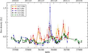
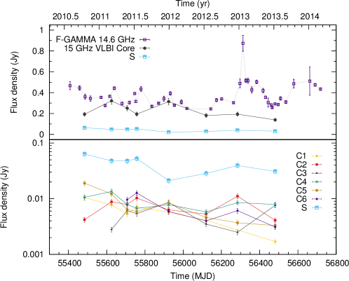
Figure 1: Single dish and VLBI radio light curves of 1H 0323+342. The top panel features the F-GAMMA total flux density light curves at 142.3, 86.2, 32.0, 14.6 and 8.35 GHz. In the middle panel, those at 14.6 GHz from EB (purple squares) along with that of the 15 GHz VLBI core (black) and the stationary component S (light blue) are shown. The bottom panel features the light curves of all individual VLBI components. Note the different scales and the presence of component S in both panels for visual comparison.

2.2 VLBI monitoring

The MOJAVE program (Lister et al. 2009) has been monitoring 1H 0323+342 with the Very Long baseline Array (VLBA) at 15 GHz between 2010 October and 2013 July, and a total of eight observing epochs of fully self-calibrated data sets are available.

The brightness distribution of the source at each epoch has been parameterised by sets of two-dimensional circular Gaussian functions with the DIFMAP package (Shepherd et al. 1994). This uses a $\chi^{2}$ minimisation algorithm (MODELFIT) to fit the parameters of the Gaussian components – i.e. flux density, radial separation from the phase center, position angle (PA) and size – to the visibility function.

First, the image of each epoch was analyzed independently by building the model iteratively, i.e. adding new components as long as the residual image shows significant flux density and the new component improved the overall fit in terms of the $\chi^{2}$ value. The addition of a component was followed by iterations of MODELFIT (until the fit has converged) and self-calibration of the visibility phases. In addition, a cross-check of our model was performed by comparing the position of the components with the brightness distribution in the CLEAN image. We adopt an uncertainty of 10% for the flux density of components (e.g. Lister et al. 2009). The positional uncertainty is set to 1/5 of the beam, if they are unresolved, or 1/5 of their FWHM for those resolved. A few data points deviate from the fitted lines, as common of such type of studies, attributable to possible epoch-to-epoch illumination of different emission regions within the same knot, and small differences in the uv-coverage. The uncertainty in PA is given by $\Delta{\rm PA}=\arctan(\Delta{\rm X}/r)$, with $\Delta{\rm X}$ the positional uncertainty and $r$ their separation from the core (e.g. Karamanavis et al. 2016). We note that neither during the cleaning nor the model-fitting process, significant flux density could be associated with a putative counter-jet above the noise-level of a given epoch (see Sect. 5). Details of the resulting multi-epoch model parameters are given in the Appendix (Table 3). All individual MODELFIT maps are shown in Fig. 2.

3 Results from total flux density monitoring

The single-dish light curves displayed in Fig. 1 (top) show 1H 0323+342 in a phase of mild, low-amplitude but rather fast variability during the period $\sim$2010 to 2012. Here, the 14.6 GHz light curve, for instance, exhibits repeated low-amplitude flares with amplitudes ($\Delta S=S_{\rm{max}}-S_{\rm{min}}$) of $\sim$120–170 mJy and time scales ($\Delta t=t_{\rm{max}}-t_{\rm{min}}$) of $\lesssim$40–100 days. Using these values, we calculate lower limits for the apparent brightness temperature $T_{\rm{B,var}}$ associated with these events ranging between $5\times 10^{10}$ and $4\times 10^{11}$ K.

Starting in 2012, the source showed more prominent activity with a first larger mm-band flare peaking around 2012.2 and subsequently, a large outburst occurring between $\sim$2012.6 and 2013.5. The latter appears to exhibit 2–3 sub-flares with the most prominent event showing a variability amplitude of $\Delta S\sim\,570$ mJy during a time period of about 50 days at 14.6 GHz. This yields a lower limit for $T_{\rm{B,var}}$ of about $9\times 10^{11}$ K. The observed brightness temperature can be further constrained using the highest significant amplitude variation occuring at adjacent times, between MJD 56296.8 and 56312.7 in the 14.6 GHz light curve (Fig. 1). This corresponds to a variability amplitude of 384 mJy and a time scale of 15.9 days. These figures yield an apparent $T_{\rm{B,var}}$ of $5.7\times 10^{12}$ K.

Assuming an intrinsic equipartition brightness temperature limit of $5\times 10^{10}$ K (Readhead 1994), we can estimate lower limits for the variability Doppler factor $D_{\rm{var}}$ required to explain the excess of $T_{\rm{B,var}}$ over the theoretical limit (e.g. Fuhrmann et al. 2008; Hovatta et al. 2009; Angelakis et al. 2015). The maximum observed value of $5.7\times 10^{12}$ K then yields $D_{\rm{var}}$ $\gtrsim$ 5.2 for the 14.6 GHz variability seen in Fig. 1. Based on a different method, their flare decomposition method, Angelakis et al. (2015) deduce a $D_{\rm{var}}$ $\gtrsim$ 3.6 for the flare seen at 14.6 GHz, peaking at MJD $\sim$56300. For a full event-by-event treatment of the data sets until Spring 2014 see the aforementioned publication.

4 Results from VLBI monitoring

Figure 2 shows the final MODELFIT maps of 1H 0323+342 at $15$ GHz. On parsec scales, the source is characterized by a one-sided jet that appears remarkably straight, oriented at a mean position angle of ${\sim}124^{\circ}$, and extending out to almost $10$ mas from its bright, unresolved core. The latter contains more than 70% of the jet’s total flux density (see Fig. 1).

As also seen in the VLBI maps of Fig. 2, the jet of 1H 0323+342 is not undisrupted all the way until its maximum angular extent. Further downstream from the core the jet exhibits an area of reduced surface brightness (a gap of emission). On average this is visible between $3$ to $6$ mas away from the core at the PA of the jet, whereafter the flow becomes visible again. This effect could be attributed to the weighting of the VLBI data, selected such that resolution is maximized at the expense of sensitivity to putative extended structure.

At our observing frequency the jet can be decomposed into six to nine MODELFIT components. Based on the parameters of the model and their temporal evolution we are able to positively cross-identify seven components between all eight observing epochs. Starting from the outermost component – in terms of radial separation from the core – we use the letter C followed by a number between $1$ and $6$ to designate and hereafter refer to them. Apart from travelling components, our findings suggest the presence of a quasi-stationary component, referred to with the letter S, positioned very close to the core at a mean distance of ${\sim}0.3$ mas. Furthermore, at epoch $2013.52$ a new component appears to emerge, most probably ejected at some time between the latest two observing epochs; i.e. between $2012.98$ and $2013.52$ (see Sect. 7.1). We refer to this knot as NC which stands for ‘new component’ (cf. VLBI maps in Fig. 2).

The kinematical properties of the jet were derived by identifying model components throughout our multi-epoch observations, which describe the same jet features. The kinematical parameters for each knot are obtained through a weighted linear regression fit of their positions relative to the assumed stationary core over time. In Fig. 3 each component’s radial separation from the core at each observing epoch is shown, along with the linear fits. From the slope of each fit we deduce the component’s proper motion $\mu$ relative to the core and its apparent velocity $\beta_{\rm app}$ in units of the speed of light. The results are summarized in Table 1.

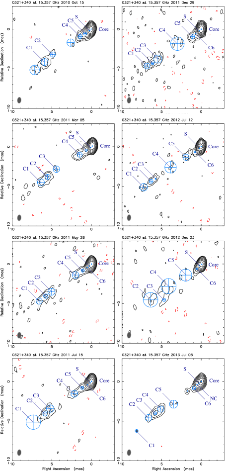
Figure 2: Eight uniformly-weighted MODELFIT maps of 1H 0323+342 from the MOJAVE observations at 15 GHz. Contour levels correspond to $-0.3$%, 0.3%, 0.6%, 1.2%, 2.4%, 4.8%, 9.6%, 19.2% and 38.4% of the highest peak flux density of 0.344 Jy beam^-1 (epoch 2011.17) for common reference. All maps are convolved with an average beam with major and minor axes of 0.77 and 0.48 mas, respectively, with the major axis at PA $=-5^{\circ}$.

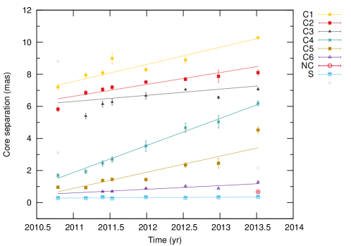
Figure 3: Temporal evolution of fitted component separation from the core. Line segments represent the best-fit linear model describing each component’s kinematical behavior. Apart from robustly-identified knots (C1–C6), open squares denote non-robust features. The new component (NC) visible in the latest epoch only, is shown as a red circle immediately after the quasi-stationary feature S.

Beyond the first mas and before the area of reduced radio emission, $\beta_{\rm app}$ shows an increasing trend. There, superluminal knots C5 and C4 travel with apparent velocities of ${\sim}4$ c and ${\sim}7$ c, respectively. Superluminal knot C4 is the fastest moving component in the relativistic flow of 1H 0323+342.

After the gap of emission, when the jet becomes visible again, the flow is characterized by slower speeds. Components C3, C2 and C1 are used to describe the elongated area of emission extending at a radial distance between 6 and 10 mas away from the core. Their speeds are superluminal, only slightly slower than in the jet area before the gap, with $\beta_{\rm app,\,C3}\simeq 1.6$, $\beta_{\rm app,\,C2}\simeq 3$, and $\beta_{\rm app,\,C1}\simeq 4$.

Ejection times of knots are derived by back-extrapolating their motion to the time of zero separation from the core and are given in the last column of Table 1. The source appears very active in this respect, showing an ejection of a new VLBI component every ${\sim}3.1$ years on average with the earliest ejection in $\sim$1994.6 and the most recent component ejections in 2009/2010.

Table 1: Kinematical parameters for all components of 1H 0323+342. Columns from left to right are: (1) component designation, (2) proper motion in mas/yr, (3) apparent velocity in units of c, (4) time of knot ejection.

ID	$\mu$	$\beta_{\rm app}$	$t_{\rm ej}$
	$({\rm mas\,yr}^{-1})$	$({\rm c})$	$({\rm yr})$
C1	$1.07\pm 0.09$	$4.38\pm 0.35$	$2003.9\pm 0.7$
C2	$0.74\pm 0.15$	$3.03\pm 0.63$	$2002.0\pm 2.1$
C3	$0.38\pm 0.26$	$1.58\pm 1.06$	$1994.6\pm 12.1$
C4	$1.69\pm 0.07$	$6.92\pm 0.29$	$2009.9\pm 0.1$
C5	$1.00\pm 0.20$	$4.12\pm 0.82$	$2010.1\pm 0.3$
C6	$0.23\pm 0.06$	$0.93\pm 0.24$	$2008.3\pm 0.9$
S	$0.02\pm 0.01$	$0.10\pm 0.05$	…

The main variable component at $15$ GHz, according to our VLBI findings, appears to be the core whereas all other VLBI jet components of 1H 0323+342 share a lower flux density level. Comparison between the F-GAMMA filled-aperture light curve at $14.6$ GHz and the VLBI total flux density of all components (see Fig. 1) indicates that VLBI flux densities account for most of the single-dish flux density, a hint that extended structure does not contribute a substancial flux density level. It in fact suggests that the total intensity flares originate in the unresolved $15$ GHz VLBI core region of the source, since the core flux density is variable and accounts for more than 70% of the observed total VLBI flux density.

5 Jet-to-counter-jet ratio

Assuming intrinsic symmetry between jet and counter-jet, the jet-to-counter-jet ratio $R$ represents the ratio of flux densities of the approaching and receding jets and is given by

$$R=\dfrac{S_{\rm Jet}}{S_{\rm cJet}}=\left(\dfrac{1+\beta\cos\theta}{1-\beta\cos\theta}\right)^{2-\alpha}=\left(\beta_{\rm app}^{2}+D^{2}\right)^{2-\alpha},$$ (1)

where $\beta$ and $\theta$ are the intrinsic speed and jet angle to the observer’s line of sight. The index ($2-\alpha$) refers to a continuous jet flow and changes to ($3-\alpha$) for a ‘blobby’ jet (Scheuer & Readhead 1979).

For the NLS1 galaxy 1H 0323+342 the total flux density of all components in the VLBA images is associated with the jet, while putative counter-jet emission from the source is not visible at the opposite direction of the core and to the North (see Fig. 2; this statement assumes, that there is no contribution from counter-jet emission to the brightest radio component). Despite the fact that there is no sign of emission from the counter-jet side, we have nonetheless tried to constrain its non-observability. First, the VLBI map with the best signal-to-noise ratio was selected, i.e. epoch 2011 March 5. Using the CLEAN algorithm (Högbom 1974) and by utilizing CLEAN windows to constrain the area where the algorithm searches for peaks, we have tried to place delta components at the opposite side of the jet in an attempts to ‘artificially create’ a fake counter-jet. Mostly positive and negative components with no significant flux (below the noise level of the map) were fitted in this area of the image – if at all – as expected. Another test was performed using the MODELFIT algorithm, this time by attempting to fit the self-calibrated (only for the phase term) visibilities with circular Gaussian components. The results were negative in this case too, with no significant components on the opposite side of the jet. Under the assumption that Doppler de-boosting is responsible for the suppression of the counter-jet one can obtain a lower limit for the jet-to-counter-jet ratio $R$. We calculate R using the MODELFIT map at epoch 2011 March 5. As an upper limit for the flux density of the counter-jet, $S_{\rm cJet}$, we take three times the rms integrated flux density, over a region with comparable size to and in the opposite side of the jet (rms $=0.38$ mJy). Being undetected, any counter-jet emission ought to be below this level. Consequently, through $R=S_{\rm Jet}/S_{\rm cJet}=S_{\rm Jet}/S_{3\sigma}$ , we estimate that $R\geq 363.5$, where $S_{\rm Jet}$ is the total integrated flux density of the fitted core and jet components.

A first estimate for the viewing angle towards the source can then be obtained through

$$\theta\leq\arccos\left(\frac{R^{\frac{1}{2-\alpha}}-1}{R^{\frac{1}{2-\alpha}}+1}\right)\hskip 5.69046pt\beta^{-1}.$$ (2)

Under the assumption that the intrinsic speed of the components of the pc-scale jet is close to the speed of light, i.e. letting $\beta\rightarrow 1$, and with a mean $\alpha=-0.04$ (Angelakis et al. 2015), we arrive at an upper limit for the viewing angle of $\theta\leq 27^{\circ}$, for $R=363.5$. If instead, we exclude the core flux density for this calculation, an even weaker constraint is obtained. Note that solving Eq. 1 for $D$, this value of $R$, combined with the highest measured apparent velocity in the jet, implies a non-physical Doppler factor ($D\in\mathbb{I}$; imaginary). To remedy this and get a real-valued Doppler factor, a much higher jet-to-counter-jet ratio is needed (${\sim}2700$), which in turn yields a viewing angle of $\theta\leq 16^{\circ}$.

Another way of constraining the viewing angle towards the source is the following. Having a measured value for $\beta_{\rm app}$ we calculate the minimum Lorentz factor in order to observe this apparent speed as

$$\gamma_{\rm min}=\sqrt{\beta_{\rm app}^{2}+1}.$$ (3)

Then using Eq. 3 under the assumption that this is the Lorentz factor characterizing the flow, the critical viewing angle is estimated through (Rees 1966)

$$\theta_{\rm crit}=\arcsin\left(\dfrac{1}{\gamma_{\rm min}}\right).$$ (4)

In this way and for $\beta_{\rm app}=6.92$, the minimum Lorentz factor is $\gamma_{\rm min}=6.99$ and correspondingly we obtain $\theta_{\rm crit}=8.2^{\circ}$. For a discussion on the use of the critical angle as a proxy for the viewing angle see Karamanavis et al. (2016).

6 The viewing angle towards 1H 0323+342

A viewing angle estimate towards 1H 0323+342 can be obtained based on our radio variability and imaging results. With regard to the obtained Doppler factor, we would first like to note, that there is, in principle, several methods for estimating Doppler factors in blazars, and NLS1 galaxies in particular. One approach is based on SED modelling, which has also been carried out for 1H 0323+342 (e.g., (Abdo et al. 2009b; Zhang et al. 2013; Paliya et al. 2014; Yao et al. 2015a; Sun et al. 2015) While this is a very important approach, the estimated parameters still come with a number of uncertainties, based on, for instance, non-simultaneity of some of the data points, assumptions about black holes mass and correspondingly the accretion disk contribution to the SED, and based on different assumptions of different authors on the dominant contribution to EC processes (like the BLR or the molecular torus, or both). Alternatively, the variability Doppler factor in the radio regime can be directly estimated from radio flux density monitoring data. We have carried out such a program over several years, and it is these data sets we have used here for directly estimating the variability Doppler factor (the value we find (Sect. 3) is consistent within the errors with estimates based on SED fitting (e.g., Yao et al. 2015a, their Tab. 6). We have performed the estimate at 15 GHz, because this is the frequency at which the VLBI data were taken.

Combining the variability Doppler factor $D_{\rm var}$ estimated in Sect. 3, based on our single-dish monitoring with the apparent jet speed $\beta_{\rm app}$ estimated in Sect. 4, we are able to estimate the variability Lorentz factor $\gamma_{\rm var}$ and the viewing angle $\theta_{\rm var}$ towards 1H 0323+342 according to (Jorstad et al. 2005, for the derivation see Onuchukwu & Ubachukwu 2013)

$$\gamma_{\rm var}=\dfrac{\beta_{\rm app}^{2}+D_{\rm var}^{2}+1}{2D_{\rm var}}~{}~{}~{}\textrm{and}$$ (5)

$$\theta_{\rm var}=\arctan\left(\dfrac{2\beta_{\rm app}}{\beta_{\rm app}^{2}+D_{\rm var}^{2}-1}\right).$$ (6)

Ideally, one aims at using the apparent jet speed of the travelling VLBI knot causing the outburst for which $D_{\rm var}$ has been obtained. However, this is not possible in the case of 1H 0323+342, given the available data sets (see also Sect. 7.1). Nevertheless, we can assume the range of obtained $D_{\rm var}$ and jet speeds in Sect. 3 and 4 as representative, average jet characteristics to obtain a range of plausible values for the Lorentz factor as well as viewing angle of the source.

Assuming a constant Doppler factor, we use Eqs. 5 and 6 and combine the observed apparent velocities of the flow with the variability Doppler factors discussed in Sect. 3. While the most stringent constraint is obtained from the combination of the lowest observed $\beta_{\rm app}=0.93$ with the highest Doppler factor, given the large scatter of observed speeds, we perform the same calculation using the lowest $D_{\rm var}\geq 3.6$ and the highest $\beta_{\rm app}=6.92$. In the former case we obtain a variability Lorentz factor $\gamma_{\rm var}\geq 2.8$ and the viewing angle $\theta_{\rm var}\leq 4.0^{\circ}$. In the latter, we have $\gamma_{\rm var}\geq 8.6$ and $\theta_{\rm var}\leq 13.0^{\circ}$. The final range of values for the viewing angle is $\theta_{\rm var}\leq 4^{\circ}$–$13^{\circ}$. Results of all calculations are summarized in Table 2.

Table 2: Physical parameters of the jet of 1H 0323+342. The left column contains the measured quantities, used in each calculation, leading to the values in the right column. The table from top to bottom contains the results with the use of VLBI data only, the critical values for the Lorentz factor (minimum value) and the viewing angle, and finally, results obtained through the combination of VLBI and single-dish data.

Measured quantities	Inferred parameters
VLBI only
$R=363.5$	$D\in\mathbb{I}$
$\beta\rightarrow 1$	$\theta\leq 27^{\circ}$
$R_{\rm req}$ = $2700$	$D\in\mathbb{R}$
$\beta\rightarrow 1$	$\theta\leq 16^{\circ}$
Critical values
$\beta_{\rm app}=6.92$	$\gamma_{\rm min}=6.99$
	$\theta_{\rm crit}=8.2^{\circ}$
VLBI and single dish
$\beta_{\rm app,min}=0.93$	$\gamma_{\rm var}\geq 2.8$
$D_{\rm var}\geq 5.2$	$\theta_{\rm var}\leq 4^{\circ}$
$\beta_{\rm app,max}=6.92$	$\gamma_{\rm var}\geq 8.6$
$D_{\rm var}\geq 3.6$	$\theta_{\rm var}\leq 13^{\circ}$

7 Discussion

7.1 On the variability of 1H 0323+342

The unresolved 15 GHz VLBI core flux density is variable and accounts for more than 70 % of the total VLBI flux density. Consequently, it is likely the region responsible for the variability and flares seen in the single-dish total flux density light curves, however, a direct connection between total flux density outbursts and pc-scale VLBI jet features cannot be established given the poor VLBI data sampling. This is particularly true for the most dramatic outburst observed around 2013.1. In addition, given the limited time baseline of the single-dish observations, we are unable to establish a one-to-one correspondence between component ejection times and total intensity flares. This becomes clear from the estimated ejection times of components reported in Table 1, none of which appears to have separated from the core within the time baseline of our single-dish radio monitoring. The only exception appears to be a new jet component (refereed to as NC) only seen to be present in the data of the last epoch ($2013.52$, see Fig. 3) with an integrated flux density of ${\sim}19$ mJy. Given the flaring activity preceding its separation from the core, this knot could be tentatively associated with the above mentioned, most dramatic outburst seen in our single-dish data around epoch ${\sim}2013.1$ (see Fig. 1).

7.2 On the viewing angle towards 1H 0323+342

A first indication that the viewing angle towards 1H 0323+342 is not exceptionally small is the remarkably straight jet. All jet components lie at a mean position angle of about 124 degrees, with minor deviations. Since the jet appears so aligned, this likely implies that the viewing angle is not too small, otherwise PA variations would be greatly enhanced and more pronounced due to relativistic aberration effects, as in the case of objects seen at very small viewing angles (${\sim}1^{\circ}$–$2^{\circ}$).

As shown in Sect. 5, the viewing angle $\theta$ towards 1H 0323+342 can be loosely constrained by using the interferometric data alone. Here, the minimum Lorentz factor estimate yields a value of $8.2^{\circ}$ from $\theta_{\rm crit}$, while the jet-to-counter-jet ratio estimate provides loose upper limits of $\theta\,\leq\,27^{\circ}$ and ultimately $\theta\,\leq\,16^{\circ}$.

The combination of VLBI kinematics and single-dish variability allows us to further constrain $\theta$ (Sect. 6). We note that the variability Doppler factors constitute only lower limits, given the fact that the emission region can be smaller than the size implied by the variability time scales obtained. Angelakis et al. (2015) presented a detailed analysis of the single-dish data sets of 1H 0323+342 between 2010.6 and 2014.2 based on a multi-frequency flare decomposition method. At 14.6 GHz, their study yielded $D_{{\rm var}}\geq 3.6$. Consequently, using $D_{{\rm var}}>3.6$ and $\beta_{\rm app}=6.92$ c we obtain a viewing angle of ${\leq}13^{\circ}$.

Additionally, in Sect. 3 we deduced a variability Doppler factor $D_{\rm var}\geq 5.2$. This, combined with the slowest apparent speed of the moving knot C6, yields another, more stringent upper limit for $\theta$ of ${\leq}4^{\circ}$. The very small apparent speed of C6 can be reconciled with such a high Doppler factor, if projection effects are at play and the jet is pointed close to the observer’s line of sight, as seen from the inferred aspect angle.

7.3 The viewing angle towards the NLS1 galaxy SBS 0846+513

Using the results presented by D’Ammando et al. (2013) (see also D’Ammando et al. 2012) we can also estimate the viewing angle towards the radio and $\gamma$-ray-loud NLS1 SBS 0846+513, using the same method presented in Sect. 6. The authors report an apparent jet speed for this source of 9.3 c. Furthermore, we estimate $D_{\rm var}$ as in Sect. 3 from the 15 GHz variability presented in Figs. 3 and 4 of D’Ammando et al. (2012) to be of the order ${\geq}6$–$7$, in agreement with a value of ${\geq}7.1$ which we obtain from the variability characteristics given in D’Ammando et al. (2013) and using an intrinsic equipartition brightness temperature limit of $5\times 10^{10}$ K. These values for $\beta_{{\rm app}}$ and $D_{\rm var}$ then provide a viewing angle estimate of ${\leq}8^{\circ}$–$9^{\circ}$ using Eq. 6.

7.4 Comparison with classical blazars

Out of the six moving features populating the jet of 1H 0323+342, five are superluminal and only one moves with a marginally subluminal velocity. The apparent velocities span a wide range between 0.93 c up to 6.92 c. Such a range of apparent speeds is often observed for the class of blazars (e.g. Lister et al. 2013).

The Lorentz factors obtained for 1H 0323+342 and SBS 0846+513 are in the observed range of blazars but at the lower end of the blazar Lorentz factor distribution and more typical for BL Lac objects (e.g. Hovatta et al. 2009; Savolainen et al. 2010).

The different methods we employ constrain the viewing angle towards 1H 0323+342 to $\theta\leq 4^{\circ}$–$13^{\circ}$, while $\theta\leq 8^{\circ}$–$9^{\circ}$ for SBS 0846+513. These numbers are larger than the average viewing angles towards blazars, of ${\sim}1^{\circ}$–$2^{\circ}$ (e.g. Hovatta et al. 2009; Savolainen et al. 2010), but given that out measurements are upper limits, the angles could still be consistent with smaller values. Whether this is a general characteristic of radio-loud, $\gamma$-ray-loud NLS1 galaxies needs to be answered by detailed studies of a larger sample of this source type.

Based on VLA observations of the kpc-scale jets of three radio-loud but non-$\gamma$-ray detected NLS1 galaxies, the finding of Richards & Lister (2015) suggest that these sources are seen at a moderate angle to the line of sight (10^∘–15^∘).

Our results confirm previous findings that radio-loud, $\gamma$-ray-loud NLS1 galaxies, as a class, share blazar-like properties. However, compared to typical GeV-blazars (e.g., Zhang et al. 2012, 2014), and references therein), most radio-loud NLS1 galaxies appear as lower brightness temperature sources, possibly seen at slightly larger viewing angles than classical blazars. These properties can then explain the typically small Doppler boosting factors and low flux densities of these sources (e.g. Fuhrmann 2010; Angelakis et al. 2015; Foschini et al. 2015; Gu et al. 2015). The application of the method presented here to a larger sample of radio-loud NLS1 galaxies will provide us with first robust measurements of the viewing angle towards this population of AGN.

8 Summary and conclusions

We have presented a VLBI study of the $\gamma$-ray- and radio-loud NLS1 galaxy 1H 0323+342, including a viewing angle measurement towards the inner jet of this source, by combining single-dish and VLBI monitoring. The salient results of our study can be summarized as follows:

1. 1H 0323+342 displays a pc-scale morphology of the core-jet type. The emission is dominated by the unresolved core which contains more than 70% of the jet’s total flux density. The jet extends straight up to about 10 mas from the bright nucleus, confirming previous results at a lower frequency. The VLBI structure at 15 GHz can be represented using six moving components and one quasi-stationary feature.

2. Five out of the six moving knots exhibit superluminal motion. The range of apparent velocities is 0.93 c up to 6.92 c. Closer to the core (${\leq}1$ mas) speeds are subluminal. Between 1 mas and 5 mas, the highest speeds of the flow are observed with components moving at about 4 c and 7 c.

3. 1H 0323+342 is active, showing flux density flares, of low to mild amplitude, but very rapid compared to the typical long-term variability of blazars. The behaviour is seen both in single-dish total flux density and on VLBI scales. Previous findings infer high brightness temperatures (above the equipartition limit) and a variability Doppler factor of 3.6, taking into account the parameters of full flaring episodes. Here we also deduce an extreme $T_{\rm B,\,var}=5.7\times 10^{12}$ K and $D_{\rm var}=5.2$, based on the most rapid variability of the highest amplitude.

4. Using different methods we ultimately constrain the viewing angle towards 1H 0323+342 to be in the range $\theta_{\rm var}\leq 4^{\circ}$–$13^{\circ}$.

5. Applying similar estimates to published results of another radio-loud NLS1 galaxy, SBS 0846+513, we estimate a viewing angle of ${\leq}8^{\circ}$–$9^{\circ}$.

Both sources are therefore seen at a small viewing angle. Taken at face value, inferred numbers are larger than the bulk of the blazar population, but still consistent with each other, given that our estimates are upper limits. Aspect angle measurements of a larger sample of radio-loud NLS1 galaxies will provide us with important new insight into orientation scenarios for NLS1 galaxies.

Appendix A MODELFIT Results

Table 3: MODELFIT results of the VLBI imaging at 15 GHz for 1H 0323+342. Columns from left to right: (1) observing epoch in fractional year, (2) integrated component flux density, (3) radial separation from the core, (4) position angle, (5) component size given as the FWHM of the major axis, (6) component identification label. C denotes the core, S the quasi-stationary component and C# the rest of the moving features. The designation ‘un’ refers to non-robustly cross-identified features.

Epoch	$S$	$r$	PA	FWHM	ID
	(Jy)	(mas)	(∘)	(mas)
2010.79	$0.193\pm 0.019$	…	…	$0.08\pm 0.01$	C
2010.79	$0.064\pm 0.006$	$0.29\pm 0.03$	$131.6\pm 6.2$	$0.16\pm 0.02$	S
2010.79	$0.019\pm 0.002$	$0.96\pm 0.08$	$127.0\pm 4.8$	$0.41\pm 0.04$	C5
2010.79	$0.011\pm 0.001$	$1.69\pm 0.11$	$123.9\pm 3.6$	$0.53\pm 0.05$	C4
2010.79	$0.002\pm 0.001$	$3.11\pm 0.19$	$123.4\pm 3.5$	$0.94\pm 0.09$	un
2010.79	$0.004\pm 0.001$	$5.82\pm 0.13$	$123.5\pm 1.3$	$0.67\pm 0.07$	C2
2010.79	$0.011\pm 0.001$	$7.21\pm 0.17$	$125.2\pm 1.4$	$0.87\pm 0.09$	C1
2010.79	$0.005\pm 0.001$	$8.81\pm 0.24$	$125.9\pm 1.6$	$1.21\pm 0.12$	C0
2011.17	$0.322\pm 0.032$	…	…	$0.10\pm 0.01$	C
2011.17	$0.048\pm 0.005$	$0.28\pm 0.02$	$131.6\pm 4.0$	$0.10\pm 0.01$	S
2011.17	$0.012\pm 0.001$	$0.93\pm 0.06$	$124.2\pm 3.8$	$0.31\pm 0.03$	C5
2011.17	$0.014\pm 0.001$	$1.94\pm 0.13$	$124.4\pm 3.8$	$0.65\pm 0.07$	C4
2011.17	$0.003\pm 0.001$	$5.39\pm 0.16$	$122.9\pm 1.7$	$0.82\pm 0.08$	C3
2011.17	$0.009\pm 0.001$	$6.85\pm 0.13$	$124.5\pm 1.1$	$0.66\pm 0.07$	C2
2011.17	$0.008\pm 0.001$	$7.95\pm 0.18$	$125.3\pm 1.3$	$0.89\pm 0.09$	C1
2011.40	$0.251\pm 0.025$	…	…	$0.10\pm 0.01$	C
2011.40	$0.048\pm 0.005$	$0.34\pm 0.02$	$135.1\pm 3.2$	$0.10\pm 0.01$	S
2011.40	$0.010\pm 0.001$	$0.68\pm 0.02$	$127.5\pm 1.6$	$0.10\pm 0.01$	C6
2011.40	$0.006\pm 0.001$	$1.38\pm 0.08$	$126.7\pm 3.4$	$0.41\pm 0.04$	C5
2011.40	$0.008\pm 0.001$	$2.45\pm 0.17$	$124.5\pm 4.0$	$0.85\pm 0.09$	C4
2011.40	$0.006\pm 0.001$	$6.15\pm 0.18$	$124.6\pm 1.7$	$0.90\pm 0.09$	C3
2011.40	$0.008\pm 0.001$	$7.06\pm 0.11$	$125.0\pm 0.9$	$0.56\pm 0.06$	C2
2011.40	$0.005\pm 0.001$	$8.09\pm 0.16$	$125.2\pm 1.1$	$0.78\pm 0.08$	C1
2011.53	$0.194\pm 0.019$	…	…	$0.10\pm 0.01$	C
2011.53	$0.053\pm 0.005$	$0.26\pm 0.02$	$133.4\pm 4.2$	$0.10\pm 0.01$	S
2011.53	$0.013\pm 0.001$	$0.70\pm 0.02$	$129.4\pm 1.6$	$0.10\pm 0.01$	C6
2011.53	$0.006\pm 0.001$	$1.45\pm 0.08$	$124.8\pm 3.1$	$0.39\pm 0.04$	C5
2011.53	$0.007\pm 0.001$	$2.69\pm 0.17$	$125.8\pm 3.6$	$0.86\pm 0.09$	C4
2011.53	$0.005\pm 0.001$	$6.27\pm 0.19$	$123.4\pm 1.7$	$0.96\pm 0.10$	C3
2011.53	$0.010\pm 0.001$	$7.19\pm 0.11$	$124.9\pm 0.9$	$0.55\pm 0.06$	C2
2011.53	$0.007\pm 0.001$	$8.99\pm 0.37$	$125.0\pm 2.3$	$1.83\pm 0.18$	C1
2011.99	$0.314\pm 0.031$	…	…	$0.10\pm 0.01$	C
2011.99	$0.021\pm 0.002$	$0.34\pm 0.02$	$129.6\pm 3.2$	$0.10\pm 0.01$	S
2011.99	$0.006\pm 0.001$	$0.89\pm 0.02$	$129.7\pm 1.2$	$0.10\pm 0.01$	C6
2011.99	$0.008\pm 0.001$	$1.44\pm 0.10$	$130.9\pm 3.9$	$0.49\pm 0.05$	C5
2011.99	$0.008\pm 0.001$	$3.53\pm 0.34$	$121.3\pm 5.5$	$1.71\pm 0.17$	C4
2011.99	$0.009\pm 0.001$	$6.66\pm 0.21$	$124.5\pm 1.8$	$1.03\pm 0.10$	C3
2011.99	$0.006\pm 0.001$	$7.52\pm 0.07$	$125.0\pm 0.6$	$0.37\pm 0.04$	C2
2011.99	$0.006\pm 0.001$	$8.29\pm 0.15$	$124.2\pm 1.0$	$0.75\pm 0.08$	C1

Epoch	S	r	PA	FWHM	ID
	(Jy)	(mas)	(∘)	(mas)
2012.53	$0.181\pm 0.018$	…	…	$0.10\pm 0.01$	C
2012.53	$0.029\pm 0.003$	$0.30\pm 0.02$	$132.8\pm 3.7$	$0.10\pm 0.01$	S
2012.53	$0.004\pm 0.001$	$1.02\pm 0.05$	$128.9\pm 2.5$	$0.23\pm 0.02$	C6
2012.53	$0.005\pm 0.001$	$2.34\pm 0.16$	$125.1\pm 3.8$	$0.78\pm 0.08$	C5
2012.53	$0.006\pm 0.001$	$4.67\pm 0.29$	$124.0\pm 3.6$	$1.46\pm 0.15$	C4
2012.53	$0.004\pm 0.001$	$7.04\pm 0.03$	$125.2\pm 0.2$	$0.15\pm 0.02$	C3
2012.53	$0.005\pm 0.001$	$7.69\pm 0.10$	$124.6\pm 0.7$	$0.50\pm 0.05$	C2
2012.53	$0.004\pm 0.001$	$8.89\pm 0.19$	$125.2\pm 1.2$	$0.96\pm 0.10$	C1
2012.98	$0.194\pm 0.019$	…	…	$0.10\pm 0.01$	C
2012.98	$0.040\pm 0.004$	$0.33\pm 0.02$	$125.5\pm 3.3$	$0.10\pm 0.01$	S
2012.98	$0.006\pm 0.001$	$0.88\pm 0.04$	$133.0\pm 2.9$	$0.22\pm 0.02$	C6
2012.98	$0.004\pm 0.001$	$2.45\pm 0.31$	$124.3\pm 7.1$	$1.53\pm 0.15$	C5
2012.98	$0.009\pm 0.001$	$5.03\pm 0.38$	$123.5\pm 4.4$	$1.92\pm 0.19$	C4
2012.98	$0.003\pm 0.001$	$6.56\pm 0.08$	$133.4\pm 0.7$	$0.41\pm 0.04$	C3
2012.98	$0.011\pm 0.001$	$7.88\pm 0.37$	$124.9\pm 2.7$	$1.85\pm 0.19$	C2
2013.52	$0.139\pm 0.014$	…	…	$0.10\pm 0.01$	C
2013.52	$0.031\pm 0.003$	$0.36\pm 0.02$	$128.5\pm 3.1$	$0.10\pm 0.01$	S
2013.52	$0.019\pm 0.002$	$0.67\pm 0.02$	$126.3\pm 1.6$	$0.10\pm 0.01$	NC
2013.52	$0.003\pm 0.001$	$1.26\pm 0.08$	$132.4\pm 3.7$	$0.41\pm 0.04$	C6
2013.52	$0.002\pm 0.001$	$2.15\pm 0.02$	$124.5\pm 0.5$	$0.10\pm 0.01$	un
2013.52	$0.003\pm 0.001$	$4.53\pm 0.21$	$129.3\pm 2.6$	$1.03\pm 0.10$	C5
2013.52	$0.008\pm 0.001$	$6.19\pm 0.16$	$124.3\pm 1.5$	$0.79\pm 0.08$	C4
2013.52	$0.008\pm 0.001$	$7.07\pm 0.08$	$124.7\pm 0.6$	$0.39\pm 0.04$	C3
2013.52	$0.004\pm 0.001$	$8.10\pm 0.17$	$124.5\pm 1.2$	$0.84\pm 0.08$	C2
2013.52	$0.002\pm 0.001$	$10.28\pm 0.08$	$127.4\pm 0.4$	$0.38\pm 0.04$	C1