Mixing of the exclusion process with small bias

Abstract.

We analyze the mixing behavior of the biased exclusion process on a path of length $n$ as the bias $\beta_{n}$ tends to $0$ as $n\to\infty$. We show that the sequence of chains has a pre-cutoff, and interpolates between the unbiased exclusion and the process with constant bias. As the bias increases, the mixing time undergoes two phase transitions: one when $\beta_{n}$ is of order $1/n$, and the other when $\beta_{n}$ is order $\log n/n$.

1. Introduction

Suppose $k$ particles are placed on vertices of the $n$-path, with no site multiply occupied. The biased exclusion process is the Markov chain $(X_{t})_{t\geq 0}$ with transitions as follows:

• choose uniformly among the $n-1$ edges of the path,

• if both vertices of the selected edge are either occupied or unoccupied, do nothing,

• if there is exactly one particle on the edge, place it on the right vertex with probability $p=(1+\beta)/2$ and on the left with probability $q=(1-\beta)/2$.

The canonical case is when $n$ is even and $k=n/2$. This defines a reversible ergodic Markov chain, which has a unique stationary distribution $\pi$. It is natural to ask about its mixing time,

$$t_{{\rm mix}}(\varepsilon)=\min\{t\geq 0\,:\,\max_{\sigma}\|{\mathbf{P}}_{\sigma}(X_{t}\in\cdot)-\pi\|_{{\rm TV}}<\varepsilon\}\,.$$

We write $t_{{\rm mix}}$ for $t_{{\rm mix}}(1/4)$. When $\beta=0$, W:MTS proved

$$\frac{1}{\pi^{2}}(1+o(1))n^{3}\log n\leq t_{{\rm mix}}(\varepsilon)\leq\frac{2}{\pi^{2}}[1+o(1)]n^{3}\log(n/\varepsilon)\,,$$

and conjectured that the lower bound is sharp. Recently, Lacoin Lacoin answered this, proving that the process has a cutoff, i.e.

$$\lim_{n\to\infty}\frac{t_{{\rm mix}}(\varepsilon)}{n^{3}\log n}\to\frac{1}{\pi^{2}}\,.$$

It is worth observing that the eigenfunction lower bound method introduced in Wilson W:MTS turns out to be widely applicable, giving sharp lower bounds for many models.

When $\beta>0$, the mixing time was first studied by BBHM, who proved $t_{{\rm mix}}=O(n^{2})$. A simpler path coupling proof was given by GPR. (This proof is repeated here as the upper bound in Theorem 9.) The purpose of this paper is to understand the mixing behavior when the bias may depend on $n$ and in particular when $\beta_{n}\to 0$ as $n\to\infty$. We show that in all cases, there is a pre-cutoff, meaning that there are universal constants $c_{1}<c_{2}$ so that

$$c_{1}\leq\frac{t_{{\rm mix}}(1-\varepsilon)}{t_{{\rm mix}}(\varepsilon)}\leq c_{2}\,.$$

We find that, depending on the rate at which $\beta\to 0$, the mixing time interpolates between the unbiased and constant bias cases.

Below summarizes our results.

We write $a_{n}\asymp b_{n}$ to mean that there exist constant $0<c_{1},c_{2}<\infty$, not depending on $\beta$, so that $c_{1}\leq a_{n}/b_{n}\leq c_{2}$.

Theorem 1.

Consider the $\beta$-biased exclusion process on $\{1,2,\ldots,n\}$ with $k$ particles. We assume that $k/n\to\rho\leq 1/2$.

1. If $n\beta\leq 1$, then

   $$t_{{\rm mix}}\asymp n^{3}\log n\,.$$ (1)

2. If $1\leq n\beta\leq\log n$, then

   $$t_{{\rm mix}}\asymp\frac{n\log n}{\beta^{2}}\,.$$ (2)

3. If $n\beta>\log n$, then

   $$t_{{\rm mix}}\asymp\frac{n^{2}}{\beta}\,.$$ (3)

We provide more precise estimates on $t_{{\rm mix}}(\varepsilon)$ in Proposition 6, Proposition 7, and Theorem 9. In particular, the lower bound in (1) follows from Proposition 6, the lower bound in (2) follows from Proposition 7, and the lower bound in (3) follows from Proposition 11. The upper bounds in (2) and (3) follow from Theorem 9, and the upper bound in (1) follows from Proposition 8.

Since the behavior of the individual particles remains diffusive in the $\beta n<1$ regime, it is not surprising that the mixing time has the same order as the unbiased process in this case. The change of the functional form of the mixing time at $\beta n=\log n$ is a more unexpected transition.

A path coupling gives useful upper bounds for $\beta\geq c/n$. When $\beta n$ is small, we use a simple coupling adapted from a coupling for (unbiased) random adjacent transpositions given in A:RWG. In the unbiased case, $k$ coupled unbiased random walks must hit zero. The bias introduced when $\beta n$ is small doesn’t overwhelm the diffusive motion, so the same idea works.

For lower bounds, when $\beta n\leq\log n$, we use Wilson’s method (introduced in W:MTS). Thus we need the eigenfunction corresponding to the second eigenvalue, which we explicitly compute. When $\beta n>\log n$, we follow the left-most particle, and show it needs at least order $n^{2}/\beta$ moves to mix.

The organization of the paper is as follows. After giving definitions in Section 2, in Section 3 we compute the eigenfunction needed for Wilson’s method, and provide the corresponding lower bounds. In particular, the lower bounds in Theorem 1 (i) and (ii) are given in Propositions 6 and 7, respectively.

We give the two upper bounds in Section 4: The upper bound in (1) is given in Proposition 8, and the other upper bounds in Theorem 1 are all immediate from Theorem 9.

We conclude with the single particle lower bound needed for Theorem 1 (iii) in Section 5.

2. Definitions

2.1. Path description

It will sometime be convenient to use a bijection of the state-space $\{0,1\}^{n}$ of the particle process to the space of nearest-neighbor paths of length $n$ which begin at $0$ and have exactly $k$ up increments and $n-k$ down increments. For a particle configuration $\sigma\in\{0,1\}^{n}$, let $h:\{0,1,\ldots,n\}\to{\mathbf{Z}}$ be defined by $h(0)=0$, and

$$h(j)-h(j-1)=(-1)^{1-\sigma(j)}\,,$$

so occupied sites correspond to increments and vacant sites correspond to decrements of the path. See Figure 1 for an illustration.

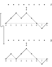
Figure 1. The correspondence between particle representation and path representation for neighboring configurations $x,y$. Node $2$ of the path is updated in configuration $x$ to obtain $y$. This corresponds to exchanging the particle at vertex $2$ with the hole at vertex $3$.

The dynamics on the path are as follows: pick among the $n-1$ interval vertices of the path. If the path is a local extremum, refresh it with a local maximum with probability $q$, and a local minimum with probability $p$. If the chosen vertex is not an extremum, do nothing. See again Figure 1 for an illustration of a transition, and Figure 2 for the possible transitions from a particular path.

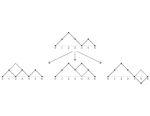
Figure 2. The possible transitions from a given configuration.

It will be convenient to move back and forth from the particle description and the path description, and we will freely do so.

3. Spectral Lower bounds

Here we set $\alpha=\sqrt{p/q}$; our assumption is always that $\alpha>1$.

Proposition 2.

Let $a(\alpha)\stackrel{{\scriptstyle def}}{{=}}(1+\alpha^{2k-n})/(1+\alpha^{-n})$. The function $\Phi$, defined for the path $h$ as

$$\Phi(h)\stackrel{{\scriptstyle def}}{{=}}\sum_{x=1}^{n-1}\Bigl{(}\alpha^{h(x)}-\alpha^{-x}a(\alpha)\Bigr{)}\sin(\pi x/n)\,,$$ (4)

is the second eigenfunction for the biased exclusion process, with eigenvalue

$$1-\frac{1-2\sqrt{pq}\cos(\pi/n)}{n-1}\,.$$

We let $\theta=q/p$; note our convention is $\theta<1$. For a path $h$ and vertex $0\leq i\leq n$, let

$$f_{h}(i)=\sum_{1\leq j\leq i}{\boldsymbol{1}}\{h(j)-h(j-1)=1\}$$

be the number of up-edges before $i$. We have $f_{h}(0)=0$ and $f_{h}(n)=k$.

Define $g^{\star}_{h}(i)=\theta^{i-f_{h}(i)}$ for $i=0,1,\ldots,n$.

Lemma 3.

Let $\tilde{h}^{(i)}$ be the path obtained by applying an update to $h$ at internal vertex $i$. Then

$${\mathbf{E}}_{h}[g^{\star}_{\tilde{h}^{(i)}}(i)]=qg^{\star}_{h}(i-1))+pg^{\star}_{h}(i+1)\,.$$ (5)

Proof.

Consider the case where $i$ is a local extremum in $h$. If the path at $i$ is refreshed to a local maximum, then $f_{\tilde{h}^{(i)}}(i)=f_{h}(i-1)+1$, while if the path is refreshed to a local minimum, then $f_{\tilde{h}^{(i)}}(i)=f_{h}(i+1)-1$. Therefore,

$${\mathbf{E}}_{h}[g^{\star}_{\tilde{h}^{(i)}}(i)]=q\theta^{i-(f_{h}(i-1)+1)}+p\theta^{i-(f_{h}(i+1)-1)}=qg^{\star}_{h}(i-1)+pg^{\star}_{h}(i+1)\,.$$

In the case where $h(i-1)<h(i)<h(i+1)$, the update at $i$ must leave the path unchanged. In this case, $f_{h}(i-1)=f_{h}(i)-1$ and $f_{h}(i+1)=f_{h}(i)+1$. Therefore,

$$qg^{\star}_{h}(i-1)+pg^{\star}_{h}(i+1)=q\theta^{i-1-(f_{h}(i)-1)}+p\theta^{i+1-(f_{h}(i)+1)}=g^{\star}_{h}(i)={\mathbf{E}}_{h}[g^{\star}_{\tilde{h}^{(i)}}]\,.$$

Finally, suppose $h(i-1)>h(i)>h(i+1)$; again, the update at $i$ does not change the path. Since $f_{h}(i-1)=f_{h}(i)=f_{h}(i+1)$ in this case,

$$qg^{\star}_{h}(i-1)+pg^{\star}_{h}(i+1)=q\theta^{(i-1)-f_{h}(i)}+p\theta^{(i+1)-f_{h}(i)}=(q\theta^{-1}+p\theta)g^{\star}_{h}(i)=g^{\star}_{h}(i)\,.$$

∎

For any constant $c$, the function $g_{h}(i)=g_{h}^{\star}(i)-c$ also satisfies

$${\mathbf{E}}_{h}[g_{\tilde{h}^{(i)}}(i)]=qg_{h}(i-1)+pg_{h}(i+1)\,.$$

Define

$$a(\theta)=\frac{1+\theta^{n/2-k}}{1+\theta^{n/2}}=\frac{1+\alpha^{2k-n}}{1+\alpha^{-n}}\,,$$

and let

$$c(n,k,\theta)=\frac{1+\theta^{n/2-k}}{1+\theta^{-n/2}}=\theta^{n/2}\Bigl{(}\frac{1+\theta^{n/2-k}}{1+\theta^{n/2}}\Bigr{)}=a(\theta)\theta^{n/2}\,.$$

Define

$$g_{h}(i)=g_{h}^{\star}(i)-c(n,k,\theta)\,.$$

Proof of Proposition 2.

Let $\phi:\{0,1,\ldots,n\}\to{\mathbf{R}}$ satisfy

$$\phi(0) =0,\quad\phi(n)=0$$

$$\lambda\phi(x) =(p\phi(x-1)+q\phi(x+1)) x=1,\ldots,n-1\,.$$

That is, $\phi$ is the eigenfunction for the $q\uparrow,p\downarrow$ random walk on $\{0,1,\ldots,n\}$ with absorbing states $0$ and $n$. A direct verification shows that

$$\phi(x)=\theta^{-x/2}\sin(\pi x/n),\quad\lambda=2\sqrt{pq}\cos(\pi/n)$$

is a solution. Note that

$$g_{h}(0)\phi(1)q+g_{h}(n)\phi(n-1)p =[1-c]\theta^{-1/2}q\sin(\pi/n)$$ (6)

$$\quad+[\theta^{n-k}-c]\theta^{-n/2}\theta^{1/2}p\sin(\pi-\pi/n)$$

$$=\sqrt{pq}\sin(\pi/n)[1+\theta^{n/2-k}-c[1+\theta^{-n/2}]]$$

$$=0\,.$$

Define

$$\Phi(h)=\sum_{x=1}^{n-1}g_{h}(x)\phi(x)\,.$$ (7)

Let $\tilde{h}$ be the configuration obtained after one step of the chain when started from $h$; as before let $\tilde{h}^{(x)}$ be the update given that internal vertex $x$ is selected for an update.

$${\mathbf{E}}_{h}[\Phi(\tilde{h})] =\sum_{x=1}^{n-1}{\mathbf{E}}_{h}[g_{\tilde{h}}(x)]\phi(x)$$

$$=\sum_{x=1}^{n-1}\Bigr{[}\Bigl{(}1-\frac{1}{n-1}\Bigr{)}g_{h}(x)+\frac{1}{n-1}{\mathbf{E}}_{h}[g_{\tilde{h}^{(x)}}]\Bigr{]}\phi(x)$$

$$=\Bigl{(}1-\frac{1}{n-1}\Bigr{)}\Phi(h)+\frac{1}{n-1}\sum_{x=1}^{n-1}[qg_{h}(x-1)+pg_{h}(x+1)]\phi(x)$$

The sum on the right equals

$$\sum_{x=1}^{n-1}g_{h}(x)[q\phi(x+1)+p\phi(x-1)]+[g_{h}(0)\phi(1)q+g_{h}(n)\phi(n-1)p]\\ =\lambda\sum_{x=1}^{n-1}g_{h}(x)\phi(x)=\lambda\Phi(h)\,,$$

by (6). Therefore,

$${\mathbf{E}}_{h}[\Phi(\tilde{h})]=\Bigl{(}1-\frac{1-\lambda}{n-1}\Bigr{)}\Phi(h)$$

Note that $\phi(x)>0$ for $x=1,\ldots,n-1$, and $g_{h}$ is increasing in $h$, so $\Phi$ is increasing. An increasing eigenfunction always corresponds to the second eigenvalue, so it must be the one with largest (non unity) eigenvalue. The second largest eigenvalue equals

$$1-\frac{1-2\sqrt{pq}\cos(\pi/n)}{n-1}\,.$$

Note that $h(x)=2f_{h}(x)-x$, so we have

$$\Phi(h) =\sum_{x=1}^{n-1}g_{h}(x)\phi(x)$$

$$=\sum_{x=1}^{n-1}\Bigl{[}\theta^{x-f_{h}(x)}-c(n,k,\theta)\Bigr{]}\theta^{-x/2}\sin(\pi x/n)$$

$$=\sum_{x=1}^{n-1}\Bigl{[}\alpha^{h(x)}-\theta^{(n-x)/2}\frac{1+\theta^{n/2-k}}{1+\theta^{n/2}}\Bigr{]}\sin(\pi x/n)$$

$$=\sum_{x=1}^{n-1}\alpha^{h(x)}\sin(\pi x/n)-\xi(n,k,\alpha)\,.$$

Let

$$\Psi(h)\stackrel{{\scriptstyle def}}{{=}}\sum_{x=1}^{n-1}\alpha^{h(x)}\sin(\pi x/n)\,.$$

Since $\xi(n,k,\alpha)$ does not depend on $h$, and the eigenfunction $\Phi$ must be orthogonal to the constants, it follows that $\xi(n,k,\alpha)=E_{\pi}(\Psi)$. Since $\sin(\pi(n-x)/n)=\sin(\pi x/n)$,

$$E_{\pi}\Psi=a(\theta)\sum_{x=1}^{n-1}\theta^{(n-x)/2}\sin(\pi x/n)=a(\theta)\sum_{x=1}^{n-1}\alpha^{-x}\sin(\pi x/n)\,.$$

∎

To apply Wilson’s Lower Bound, we need to bound $\max_{h}\Phi(h)$ from below, and $R:=|(\Phi(\tilde{h})-\Phi(h))|^{2}$ from above. Define

$$h_{0}(x)=\begin{cases}x&x\leq k\\ 2k-x&k<x\leq n\,.\end{cases}$$ (8)

Lemma 4.

For $h_{0}$ defined in (8),

$$\begin{split}\Phi(h_{0})&=\sum_{x=1}^{k}\alpha^{x}(1-\alpha^{-2x})a(\alpha)\sin(\pi x/n)\\ &\quad+\sum_{x=k+1}^{n/2}\alpha^{x}\Bigr{(}\frac{(\alpha^{2k}-1)(\alpha^{-2x}+\alpha^{-n})}{1+\alpha^{-n}}\Bigr{)}\sin(\pi x/n)\,.\end{split}$$ (9)

Proof.

Using that $\sin(\pi x/n)=\sin(\pi(n-x)/n)$, we pair together the terms at $x$ and $n-x$ in (4) so that

$$\Phi(h_{0}) =\sum_{x=1}^{k}\left(\alpha^{x}+\alpha^{2k-n+x}-a(\alpha)(\alpha^{-x}+\alpha^{x-n})\right)\sin(x\pi/n)$$

$$\quad+\sum_{x=k}^{n/2}\left(\alpha^{2k-x}+\alpha^{2k-n+x}-a(\alpha)(\alpha^{-x}+\alpha^{x-n})\right)\sin(x\pi/n)\,.$$

The first sum simplifies to

$$\sum_{x=1}^{k}\alpha^{x}(1-\alpha^{-2x})\Bigl{(}\frac{1+\alpha^{2k-n}}{1+\alpha^{-n}}\Bigr{)}\sin(\pi x/n)\,,$$

and the second to

$$\sum_{x=k+1}^{n/2}\alpha^{x}\Bigr{(}\frac{(\alpha^{2k}-1)(\alpha^{-2x}+\alpha^{-n})}{1+\alpha^{-n}}\Bigr{)}\sin(\pi x/n)\,.$$

∎

Lemma 5.

Let $h_{0}$ be as in (8), and for a path $h$, let $\tilde{h}$ be one step of the exclusion chain started from $h$. Let $\gamma=1-\lambda$ be the spectral gap. Define

$$R\stackrel{{\scriptstyle def}}{{=}}\max_{h}|\Phi(\tilde{h})-\Phi(h)|^{2}\,.$$

If $0<n\beta\leq\log n$, then

$$\log\Bigl{(}\frac{\gamma\Phi(h_{0})^{2}}{2R}\Bigr{)}\geq[1+o(1)]\log n\,.$$

Proof.

Fix $b<k$. From (9),

$$\Phi(h_{0}) \geq\frac{\sin(\pi b/n)}{2}\sum_{x=b}^{k}\alpha^{x}(1-\alpha^{-2x})$$

$$=\frac{\sin(\pi b/n)}{2}\alpha^{k}\frac{(\alpha-\alpha^{-(k-b)})(1-\alpha^{-(b+k)})}{\alpha-1}\,.$$ (10)

If $\tilde{h}$ is obtained by a single update to $h$ at $x$, the $|\tilde{h}(x)-h(x)|\leq 2$, and

$$|\alpha^{h(x)}-\alpha^{\tilde{h}(x)}|\leq 2\alpha^{k}\log(\alpha)\,.$$

Thus, if $R=\max_{h}|\Phi(\tilde{h})-\Phi(h)|^{2}$, then

$$\sqrt{R}\leq 2\alpha^{k}(\alpha-1)\,.$$ (11)

Letting $b=k/2$ so that $b/n\to\rho/2$, equations (10) and (11) show that

$$\frac{\Phi(h_{0})^{2}}{2R}\geq c_{0}\left[\frac{(\alpha-\alpha^{-k/2})(1-\alpha^{-3k/2})}{(\alpha-1)^{2}}\right]^{2}\,.$$ (12)

The spectral gap $1-\lambda=\gamma$ satisfies

$$\gamma =\frac{1-2\sqrt{pq}\cos(\pi/n)}{n-1}$$

$$=\frac{\beta^{2}/2+O(\beta^{4})+\frac{\pi^{2}}{2n^{2}}+O(n^{-4})}{n-1}\,.$$ (13)

Suppose that $n^{-1}\leq\beta\leq\frac{\log n}{n}$. Then from (12) and (13) we have

$$\log\Bigl{(}\frac{\gamma\Phi(h_{0})^{2}}{2R}\Bigr{)}\geq\log\Bigl{(}c_{1}\frac{n}{\log^{4}n}\Bigr{)}=[1+o(1)]\log n\,.$$

If $n\beta\to\zeta$, where $0\leq\zeta\leq 1$, then

$$\liminf_{n\to\infty}\frac{\gamma\Phi(h_{0})^{2}}{n2R}\geq\begin{cases}c_{0}\left[\frac{(1-e^{-\zeta\rho/2})(1-e^{-3\zeta\rho/2})}{\zeta^{2}}\right]^{2}&\zeta>0\\ c_{0}\left(\frac{3\rho^{2}}{4}\right)^{2}&\zeta=0\end{cases}\,.$$

The right-hand side is bounded below for $0\leq\zeta\leq 1$, so we conclude that

$$\log\Bigl{(}\frac{\gamma\Phi(h_{0})^{2}}{2R}\Bigr{)}\geq[1+o(1)]\log n\,.$$

∎

Proposition 6.

If $n\beta\to\zeta$ where $0\leq\zeta$, then

$$t_{{\rm mix}}(\varepsilon)\geq\frac{n^{3}}{\pi^{2}+\zeta^{2}}[1+o(1)]\Bigl{(}\log n+\log[(1-\varepsilon)/\varepsilon)]\Bigr{)}\,.$$ (14)

Proof.

From (13), the spectral gap $1-\lambda=\gamma$ satisfies

$$\gamma=\frac{\pi^{2}+\zeta^{2}}{2n^{3}}[1+o(1)]\,.$$

Using Lemma 5 in W:MTS (see also Theorem 13.5 of LPW for a discussion) yields

$$t_{{\rm mix}}(\varepsilon) \geq\frac{1}{2\log(1/\lambda)}\left[\log\left(\frac{(1-\lambda)\Phi(x)^{2}}{2R}\right)+\log((1-\varepsilon)/\varepsilon)\right]$$ (15)

$$=\frac{n^{3}}{(\pi^{2}+\zeta^{2})}[1+o(1)]\Bigl{(}\log n+\log[(1-\varepsilon)/\varepsilon]\Bigr{)}\,,$$

which yields (14). Note that this matches the lower bound in Theorem 4 of Wilson (2004) for the symmetric exclusion when $\lim_{n}\beta n=0$. ∎

Proposition 7.

If $n\beta\to\infty$ but $n\beta\leq\log n$, then

$$t_{{\rm mix}}(\varepsilon)\geq\frac{n}{\beta^{2}}[1+o(1)](\log n+\log[(1-\varepsilon)/\varepsilon])\,.$$

Proof.

This again follows from (13), (15) and Lemma 5. ∎

4. Upper Bounds

4.1. Nearly unbiased

Proposition 8.

There exists a constant $c_{1}$ such that if $n\beta\leq 1$, then

$$t_{{\rm mix}}(\varepsilon)\leq c_{1}n^{3}\log n\,.$$

Proof.

We now define a Markov chain $(\sigma_{t},\eta_{t})$ so that

• $\sigma_{t}$ and $\eta_{t}$ are labelled $k$-particle configurations,

• if the labels are erased, $(\sigma_{t})$ and $(\eta_{t})$ each are biased exclusion processes.

We say a labelled particle is coupled at time $t$ if it occupies the same vertex in both $\sigma_{t}$ and $\eta_{t}$.

We now describe a move of this chain from state $(\sigma,\eta)$: Pick an edge $e$ among the $n-1$ edges uniformly at random. We consider several cases.

• Both $\sigma$ and $\eta$ have no particles on $e$. The chain remains at $(\sigma,\eta)$.

• One of $\sigma,\eta$ contains two particles on $e$, and one of $\sigma,\eta$ contains one particle on $e$. Suppose, without loss of generality, that $\sigma$ contains one particle on $e$. Toss a $p$-coin to determine where the particle is placed in $\sigma$. If the single particle on $e$ in $\sigma$ is coupled, or has the same label as one of the particles on $e$ in $\eta$, arrange the two particles on $e$ in $\eta$ to preserve or facilitate the coupling. Otherwise, toss a fair coin to determine the placement of the two particles in $\eta$.

• Both $\sigma$ and $\eta$ have two particles on $e$. Toss a fair coin to determine the placement of the two particles on $e$ in $\sigma$. Place the particles in $\eta$ on $e$ to preserve or facilitate any couplings; if no coupling is possible, toss a fair coin to determine the particle placement on $e$.

The distance $D_{i}(t)$ between particle $i$ in $\sigma$ and particle $i$ in $\eta$ performs a delayed nearest-neighbor walk, with possible bias $\beta$ at each move (sometimes the bias is to the right, sometimes to the left). The probability it moves is at least $1/(n-1)$. We can thus couple it to a random walk $(S_{t})$ with constant upward bias $\beta$ so that $D_{i}(t)\leq S_{t}$ until $D_{i}(t)$ hits zero.

Consider the biased random walk $(S_{t})$ on ${\mathbf{Z}}$ with positive bias $\beta$, holding probability $1-\frac{1}{n-1}$, and $S_{0}=n$; if

$$\tau=\min\{t\geq 0\,:\,S_{t}=0\}\,,\quad\text{ and }\tau_{i}=\min\{t\geq 0\,:\,D_{i}(t)=0\}\,,$$

then

$${\mathbf{P}}(\tau_{i}>u)\leq{\mathbf{P}}(\tau>u)\,.$$

We have

$${\mathbf{P}}(\tau\leq t)\geq{\mathbf{P}}_{n}(S_{t}\leq 0)\\ ={\mathbf{P}}\left(Z_{t}\leq\frac{-n-t\beta/(n-1)}{\sqrt{4tpq/(n-1)}}\right)$$

where $Z_{t}=\frac{S_{t}-{\mathbf{E}}_{n}(S_{t})}{\operatorname{Var}(S_{t})}$. By the Central Limit Theorem, since $\beta n\leq 1$, there is a constant $c_{0}>0$ such that, for $n$ large enough,

$${\mathbf{P}}_{n}(S_{n^{3}}\leq 0)\geq c_{0}\,.$$

Thus by taking $c_{1}$ large enough,

$${\mathbf{P}}_{n}(\tau>c_{1}n^{3})\leq(1-c_{0})^{c_{1}}<\frac{1}{2}\,.$$

If we run $2\log_{2}n$ blocks of $c_{1}n^{3}$ moves, then we have

$${\mathbf{P}}(\tau_{i}>2c_{1}n^{3}\log_{2}n)\leq\frac{1}{n^{2}}\,.$$

Setting $\tau_{{\rm couple}}\stackrel{{\scriptstyle def}}{{=}}\min\{t\geq 0\;:\;\sigma_{t}=\eta_{t}\}$,

$${\mathbf{P}}\bigl{(}\tau_{{\rm couple}}>2c_{1}n^{3}\log_{2}n\bigr{)}\leq\sum_{i=1}^{k}{\mathbf{P}}(\tau_{i}>2c_{1}n^{3}\log_{2}n)<\frac{1}{n}\,.$$

If $d(t)=\sup_{h}\|P^{t}(h,\cdot)-\pi\|_{{\rm TV}}$, then $d(2c_{1}n^{3}\log_{2}n)\leq\frac{1}{n}$, and

$$t_{{\rm mix}}(\varepsilon)\leq 2c_{1}n^{3}\log_{2}n$$

for $n$ large enough. ∎

4.2. Path coupling

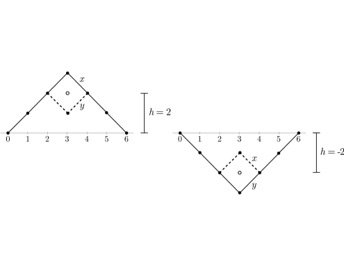
Figure 3. Neighboring configurations $x$ and $y$.

We consider configurations $x$ and $y$ to be adjacent if $y$ can be obtained from $x$ by taking a particle and moving it to an adjacent unoccupied site. In the path representation, moving a particle to the right corresponds to changing a local maximum (i.e., an “up-down”) to a local minimum (i.e. a “down-up”). Moving a particle to the left changes a local minimum to a local maximum. See Figure 1, where $v=3$.

Theorem 9.

Consider the biased exclusion process with bias $\beta=\beta_{n}=2p_{n}-1>0$ on the segment of length $n$ and with $k$ particles. Set $\alpha=\sqrt{p_{n}/(1-p_{n})}$. For $\varepsilon>0$, if $n$ is large enough, then

$$t_{{\rm mix}}(\varepsilon)\leq\frac{2n}{\beta^{2}}\left[\log(1/\varepsilon)+\log\left[\frac{\alpha(\alpha^{k}-1)(\alpha^{n-k}-1)}{(\alpha-1)^{2}}\right]\right]\,.$$

In particular, if $\beta\leq{\rm const.}<1$, then $\alpha=1+\beta+O(\beta^{2})$, so

$$t_{{\rm mix}}(\varepsilon)\leq\frac{2n}{\beta^{2}}\Bigl{[}\log(\varepsilon^{-1})+n[\beta+O(\beta^{2})]-2\log\beta+O(\beta)\Bigr{]}\,.$$

Remark 10.

Note that whenever $c_{1}(\log n)/n<\beta<c_{2}<1$ for constants $c_{1}$ and $c_{2}$, the ratio of the upper and lower bounds is bounded. Thus there is a pre cut-off for this chain in this regime.

Proof.

For $\alpha=\sqrt{p/q}>1$, define the distance between two configurations $x$ and $y$ which differ by a single transition to be

$$\ell(x,y)=\alpha^{n-k+h},$$

where $h$ is the height of the midpoint of the diamond that is removed or added. (See Figure 3.) Note that $\alpha>1$ and $h\geq-(n-k)$ guarantee that $\ell(x,y)\geq 1$, so we can use path coupling – see, e.g., Theorem 14.6 of LPW. We again let $\rho$ denote the path metric on ${\mathcal{X}}$ corresponding to $\ell$.

We couple from a pair of initial configurations $x$ and $y$ which differ at a single vertex $v$ as follows: choose the same vertex in both configurations, and propose a local maximum with probability $1-p$ and a local minimum with probability $p$. For both $x$ and $y$, if the current vertex $v$ is a local extremum, refresh it with the proposed extremum; otherwise, remain at the current state.

Let $(X_{1},Y_{1})$ be the state after one step of this coupling. There are several cases to consider.

The first case is shown in Figure 3. Let $x$ be the upper configuration, and $y$ the lower. Here the edge between $v-2$ and $v-1$ is “up”, while the edge between $v+1$ and $v+2$ is “down”, in both $x$ and $y$. If $v$ is selected, the distance decreases by $\alpha^{n-k+h}$. If either $v-1$ or $v+1$ is selected, and a local minimum is selected, then the lower configuration $y$ is changed, while the upper configuration $x$ remains unchanged. Thus the distance increases by $\alpha^{n-k+h-1}$ in that case. We conclude that

$${\mathbf{E}}_{x,y}[\rho(X_{1},Y_{1})]-\rho(x,y) =-\frac{1}{n-1}\alpha^{h+n-k}+\frac{2}{n-1}p\alpha^{h+n-k-1}$$

$$=\frac{\alpha^{h+n-k}}{n-1}\left(\frac{2p}{\alpha}-1\right)=\frac{\alpha^{h+n-k}}{n-1}\left(2\sqrt{pq}-1\right)\,.$$ (16)

In the case where $x$ and $y$ at $v-2,v-1,v,v+1,v+2$ are as in the right panel of Figure 3, we obtain

$${\mathbf{E}}_{x,y}[\rho(X_{1},Y_{1})]-\rho(x,y) =-\frac{1}{n-1}\alpha^{h+n-k}+\frac{2}{n-1}(1-p)\alpha^{h+n+1}$$

$$=\frac{\alpha^{h+n-k}}{n-1}\left(2\alpha(1-p)-1\right)=\frac{\alpha^{h+n-k}}{n-1}\left(2\sqrt{pq}-1\right)$$ (17)

(We create an additional disagreement at height $h+1$ if either $v-1$ or $v+1$ is selected and a local maximum is proposed; the top configuration can accept the proposal, while the bottom one rejects it.) Since $p>1/2$, we have $\delta\stackrel{{\scriptstyle def}}{{=}}1-2\sqrt{pq}>0$, and both (16) and (17) reduce to

$${\mathbf{E}}_{x,y}[\rho(X_{1},Y_{1})]-\rho(x,y)=-\frac{\alpha^{h+n-k}}{n-1}\delta\,.$$ (18)

Now consider the case on the left of Figure 4. We have

$${\mathbf{E}}_{x,y}[\rho(X_{1},Y_{1})]-\rho(x,y) =-\frac{1}{n-1}\alpha^{h+n-k}+\frac{1}{n-1}q\alpha^{h+n-k+1}+\frac{1}{n-1}p\alpha^{h+n-k-1}$$

$$=\frac{\alpha^{h+n-k}}{n-1}\left(q\alpha+\frac{p}{\alpha}-1\right)$$

$$=-\frac{\alpha^{h+n-k}}{n-1}\delta\,,$$

which gives again the same expected decrease as (18). (In this case, a local max proposed at $v-1$ will be accepted only by the top configuration, and a local min proposed at $v+1$ will be accepted only by the bottom configuration.) The case on the right of Figure 4 is the same.

Thus, (18) holds in all cases. That is, since $\rho(x,y)=\ell(x,y)=\alpha^{h+n-k}$,

$${\mathbf{E}}_{x,y}[\rho(X_{1},Y_{1})]=\rho(x,y)\left(1-\frac{\delta}{n-1}\right)\leq\rho(x,y)e^{-\frac{\delta}{n-1}}\,.$$

The diameter of the state-space is the distance from the configuration with $k$ “up” edges followed by $n-k$ “down” edges to the configuration with $n-k$ “down edges” followed by $k$ “up” edges. To move from the former to the latter, first flip the top-most maxima, next the subsequent two maxima, continuing down $k-1$ levels. At level $j$, there are $j$ maxima to flip. Each of the next $n-2k+1$ levels will have $k$ maxima to flip. The number of maxima in the last $k-1$ levels decrease by a unit at each depth. Thus, the distance travelled equals

$$\sum_{j=1}^{k-1}j\alpha^{n-k+k-j}+\sum_{j=k}^{n-k}k\alpha^{n-k+k-j}+\sum_{j=n-k+1}^{n-1}(n-j)\alpha^{n-k+k-j}$$

$$=\frac{\alpha(\alpha^{k}-1)(\alpha^{n-k}-1)}{(\alpha-1)^{2}}$$

Since $\delta\geq\beta^{2}/2$, Corollary 14.7 of LPW gives

$$t_{{\rm mix}}(\varepsilon)\leq\frac{2n}{\beta^{2}}\left[\log(1/\varepsilon)+\log\left[\frac{\alpha(\alpha^{k}-1)(\alpha^{n-k}-1)}{(\alpha-1)^{2}}\right]\right]\,.$$

Note that $\alpha=1+\beta+O(\beta^{2})$ as $\beta\to 0$, so

$$t_{{\rm mix}}(\varepsilon)\leq\frac{2n}{\beta^{2}}\left[\log(\varepsilon^{-1})+n[\beta+O(\beta^{2})]-2\log\beta+O(\beta)\right]\,.$$

In particular, if $\beta=\frac{1}{n}$, then $t_{{\rm mix}}(\varepsilon)=O(n^{3}\log n)$, which is the same order as the mixing time in the symmetric case.

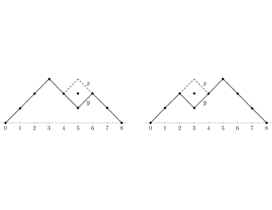
Figure 4. More neighboring configurations.

∎

5. Lower bound via a single particle

Proposition 11.

Suppose that $n\beta\to\infty$. For any $\varepsilon>0$ and $\delta>0$, if $n$ is large enough, then

$$t_{{\rm mix}}(\varepsilon)\geq\frac{(1-\delta)n^{2}}{2\beta}\,.$$

Proof.

We use the particle description here. The stationary distribution is given by

$$\pi(x)=\frac{1}{Z}\prod_{i=1}^{k}\left(\frac{p}{q}\right)^{z_{i}(x)}=\frac{1}{Z}(p/q)^{\sum_{i=1}^{k}z_{i}(x)},$$

where $(z_{1}(x),\ldots,z_{k}(x))$ are the locations of the $k$ particles in the configuration $x$, and $Z$ is a normalizing constant. To see this, if $x^{\prime}$ is obtained from $x$ by moving a particle from $j$ to $j+1$, then

$$\frac{\pi(x)P(x,x^{\prime})}{\pi(x^{\prime})P(x^{\prime},x)}=\frac{1}{(p/q)}\frac{\frac{1}{n-1}p}{\frac{1}{n-1}q}=1\,.$$

Let $L(x)$ be the location of the left-most particle of the configuration $x$, and let $R(x)$ be the location of the right-most unoccupied site of the configuration $x$.

Let

$${\mathcal{X}}_{j,\ell}=\{x\,:\,L(x)=j,\;R(x)=\ell\}\,,$$

and consider the transformation $T:{\mathcal{X}}_{j,\ell}\to{\mathcal{X}}$ which takes the particle at $j$ and moves it to $\ell$. Note that $T$ is one-to-one on ${\mathcal{X}}_{j,\ell}$.

We have

$$\pi({\mathcal{X}}_{j,\ell})\left(\frac{p}{q}\right)^{\ell-j}\leq\sum_{x\in{\mathcal{X}}_{j,\ell}}\pi(T(x))\leq 1\,,$$

so

$$\pi({\mathcal{X}}_{j,\ell})\leq\alpha^{-2(\ell-j)}\,.$$

Letting $G=\{x\,:\,L(x)\leq(1/2-b)n\}$, we have

$$\pi(G)\leq\sum_{{j\leq(1/2-b)n,\;\ell\geq n/2}}\pi({\mathcal{X}}_{j,\ell})\leq n^{2}\alpha^{-bn}\,.$$

We consider now starting from a configuration $x_{0}$ with $L(x_{0})=bn/2$.

The trajectory of the left-most particle, $(L_{t})$, can be coupled with a delayed biased nearest-neighbor walk $(S_{t})$ on ${\mathbf{Z}}$, with $S_{0}=bn/2$ and such that $L_{t}\leq S_{t}$, as long as $S_{t}>1$. The holding probability for $(S_{t})$ equals $1-\frac{1}{n-1}$. By the gambler’s ruin, the chance $S_{t}$ ever reaches $1$ is bounded above by

$$(q/p)^{bn/2}\leq e^{-\beta bn}\,.$$

Therefore.

$${\mathbf{P}}_{x_{0}}\{L_{t}>(1/2-b)n\}\leq e^{-\beta bn}+{\mathbf{P}}_{bn/2}\{S_{t}>(1/2-b)n\}\,.$$ (19)

By Chebyshev’s Inequality (recalling $S_{0}=bn/2$),

$${\mathbf{P}}\{|S_{t}-bn/2-\beta t/(n-1)|>M\}\leq\frac{\operatorname{Var}(S_{t})}{M^{2}}\leq\frac{t}{M^{2}(n-1)}\,.$$

Taking $t_{n}=\frac{(1-4b)(n-1)n/2}{\beta}$ and $M=bn/2$ shows that

$${\mathbf{P}}_{bn/2}\{S_{t_{n}}>(1/2-b)n\}\leq\frac{4(1-4b)}{b^{2}\beta n}\to 0\,,$$

as long as $\beta n\to\infty$. Combining with (19) shows that

$${\mathbf{P}}\{L_{t_{n}}>(1/2-b)n\}\leq e^{-b\beta n}+o(1)\,.$$

We conclude that as long as $\beta n\to\infty$,

$$d(t_{n})\geq{\mathbf{P}}_{x_{0}}\{X_{t_{n}}\in G\}-\pi(G)\geq 1-o(1)$$

as $n\to\infty$, whence $t_{{\rm mix}}(\varepsilon)\geq\frac{(1-4b)(n-1)n}{2\beta}$ for sufficiently large $n$.

∎