Phase transition from egalitarian to hierarchical societies driven by competition between cognitive and social constraints

Abstract

Empirical evidence suggests that social structure may have changed from hierarchical to egalitarian and back along the evolutionary line of humans. We model a society subject to competing cognitive and social navigation constraints. The theory predicts that the degree of hierarchy decreases with encephalization and increases with group size. Hence hominin groups may have been driven from a phase with hierarchical order to a phase with egalitarian structures by the encephalization during the last two million years, and back to hierarchical due to fast demographical changes during the Neolithic. The dynamics in the perceived social network shows evidence in the egalitarian phase of the observed phenomenon of Reverse Dominance. The theory also predicts for modern hunter-gatherers in mild climates a trend towards an intermediate hierarchy degree and a phase transition for harder ecological conditions. In harsher climates societies would tend to be more egalitarian if organized in small groups but more hierarchical if in large groups. The theoretical model permits organizing the available data in the cross-cultural record (Ethnographic Atlas, N=248 cultures) where the symmetry breaking transition can be clearly seen.

I Introduction

Behavioral phylogenetics makes it plausible that the common ancestor of Homo and Pan genera had a hierarchical social structure Knauft1991 ; Boehm1999 ; Boehm12 ; Dubreuil ; Dubreuilbook . Paleolithic humans with a foraging lifestyle, however, most likely had a largely egalitarian society and yet hierarchical structures became again common in the Neolithic period. Contemporary illiterate societies fill the ethological spectrum Vehrencamp1983 from egalitarian to authoritarian and despotic. This non-monotonic journey, a so called U-shaped trajectory, along the egalitarian-hierarchical spectrum during human evolution, was stressed by Knauft Knauft1991 and has defied theory despite several attempts of anthropological explanation Knauft1991 . Our approach to the study of social organization uses tools of information theory and statistical mechanics. It is inspired in previous work by Terano et al. terano2008 ; terano2009 on a different problem, the emergence of money in a barter society as a consequence of limited cognitive capacity. We model the perception by each agent of the social network of its society, taking into account cognitive constraints and social navigation demands, which define the informational constraints adequate to a probabilistic description. According to the model, whether an egalitarian-symmetric or hierarchical-broken symmetry state occurs depends on a scaling parameter which grows with cognitive capacity and decreases with group size, modulated by a Lagrange multiplier which can be interpreted as an environmental pressure. The hypothesis that social perceptions mediate motivations and hence possible behaviors (PMB hypothesis), permits making predictions about the effect of these variables in the probable forms of social organization. Since there was a massive increase in encephalic mass in the last two million years, our theory expects a phase transition towards a more egalitarian social organization to occur. As food producing and storage methods permitted the populational increase in the Neolithic, the scaling parameter decrease permitted a reversal to hierarchical structures.

Furthermore, the same model makes predictions about a totally different empirical situation, dealing with the influence of ecology on the expected hierarchy of modern human groups. The theory suggests a form of looking at the available ethnographic data ethnoatlas ; Murdock2006 and allows a new interpretation of observed patterns involving social structure, community size and environment in terms of a competition between cognitive constraints and social navigation demands and a symmetry breaking phase transition. The bifurcation suggested by the theory is seen in the ethnographic records. The empirical data can be found in the Murdock’s Ethnographic Atlas ethnoatlas , which resulted from the tour de force attempt to compile all ethnographic available knowledge that can be represented in a quantitative form.

We are studying the properties of finite size groups and so cannot take the thermodynamic limit. The changes in behavior are therefore not singular but we still find that the language of phase transitions is adequate, after all from a technical point of view the infinite size limit is a tool to simplify the mathematical treatment of very large systems.

II The theory and the model

In a group of $n$ agents, each agent of the group will have a perceived social web of interactions represented by a graph. An important distinction has to be made between the social network, that say an ethnographer might describe and the perceived social network of a particular agent. Each vertex of a graph stands for a represented agent of the group. In this representation of the social web, undirected edges joining any pair of vertices might be present or not. An edge links two represented agents if their social relation is known by the owner of the graph. Since inference depends on the available information, these graphs might differ from agent to agent. Call ${\bf S}^{i}$ the representation of the social web by agent $i$, given by a set $\{s^{i}_{jk}\}$ of variables that can take values either zero or one. The indices $i,j$ and $k$ run from $1$ to $n$ and every $s^{i}_{jk}$ is symmetric with respect to interchange of the lower indices. If $s^{i}_{jk}=1$ then agent $i$ has knowledge of the social relation, the capacity to cooperate and form coalitions or the antagonism between agents $j$ and $k$, while if $s^{i}_{jk}=0$ this relation is unknown to agent $i$. Known alliances, feuds or neutral interactions are represented by $s^{i}_{jk}=1$. The total number of memorized social relations is

$$N^{i}_{cog}=\sum_{j,k=1}^{n}s^{i}_{jk}/2$$ (1)

the number of edges in the social web representation of agent $i$. This is a cognitive contribution to the cost of a given representation ${\bf S}^{i}$.

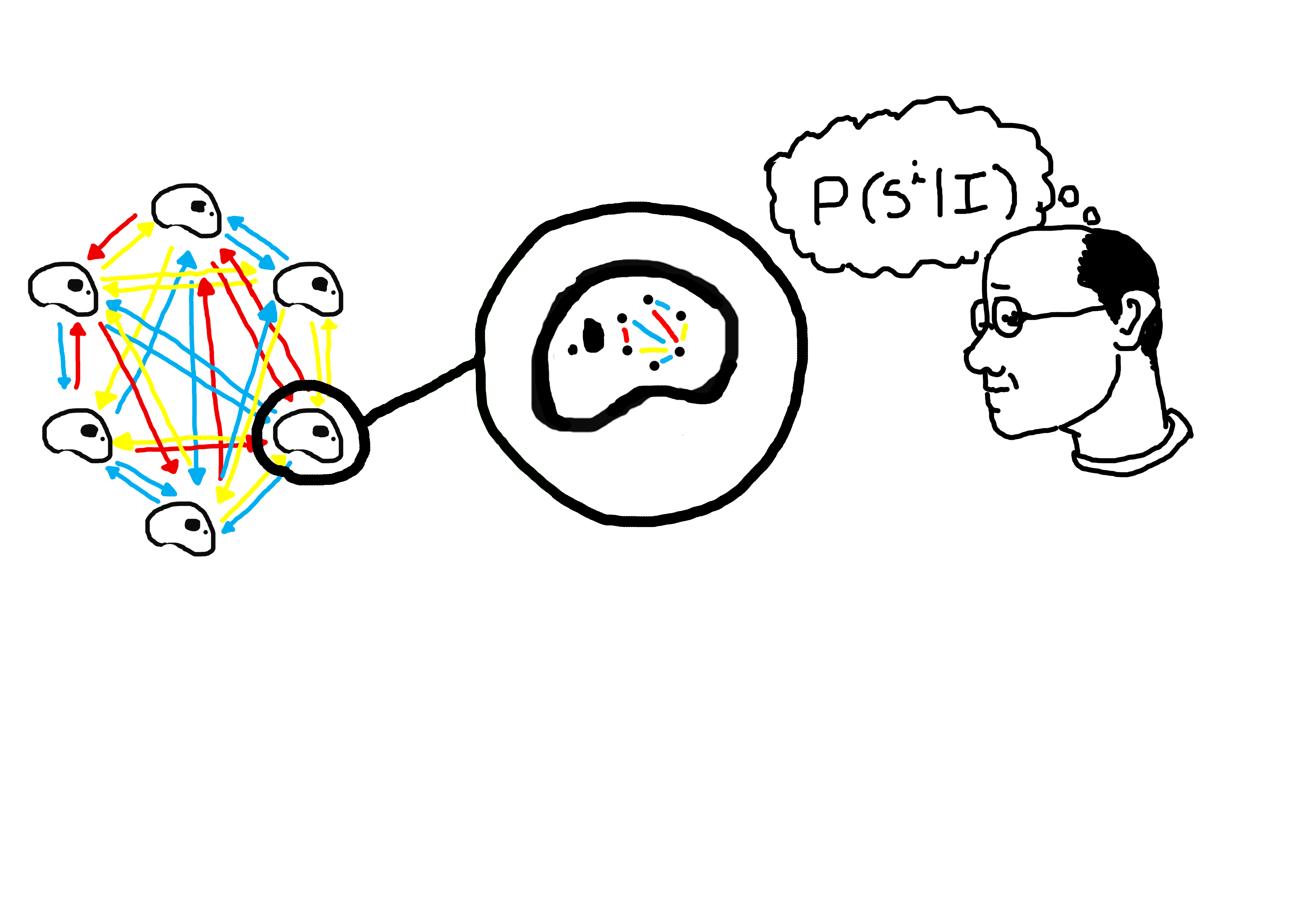
Figure 1: Each agent has a perceived social web of interactions represented by a graph. Each vertex of a graph stands for a represented agent of the group. An edge in this perceived web links two agents if their social relation is known by the owner of the graph. Using the methods of information theory entropic inference, we attribute a probability $P({\bf S}^{i}|I)$ that agent $i$ perceives a network $S^{i}$, conditional on any available information $I$.

Now consider the agent $i$’s social cost for not knowing a given social relationship, when $s^{i}_{jk}=0$. For two agents $j$ and $k$ there is either a bond or a path of bonds, joining intervening agents, connecting them so that their social relation can be estimated by agent $i$. We will assume that the representation is a connected graph, what can be accomplished by defining the distance of two unconnected vertices to be infinite. It is reasonable to assume that this lack of direct knowledge will imply in a social cost which increases with the length of the shortest path between the agents. This implements the idea that relying on heuristics to infer the relationship between them (e.g., “a friend of an enemy is an enemy”, etc.) is more amenable to errors as the number of intermediate agents grows.

Call $l^{i}_{jk}$ the social distance in the graph defined by the adjacency matrix ${\bf S}^{i}$. The $\lambda-$th power of ${\bf S}^{i}$,

$$\,{\bf M}^{i}(\lambda)=[{\bf S}^{i}]^{\lambda}$$

permits verifying whether there is a path joining two agents, and the social distance is

$$l^{i}_{jk}={\tt min}\,\lambda,\mbox{such that }{\bf M}^{i}(\lambda)_{jk}>0$$

is the length of the smallest path of bonds linking $j$ and $k$. We take the social cost of agent $i$ of having a representation ${\bf S}^{i}$ to be just the distance averaged over all pairs of agents

$$\bar{L^{i}}=\frac{2}{n(n-1)}\sum_{j,k=1}^{n}l^{i}_{jk}.$$ (2)

The joint cognitive-social cost of the representation is defined as a sum of monotonic functions of $N^{i}_{cog}$ and $\bar{L^{i}}$ and the simplest form is just

$$C_{0}({\bf S}^{i})=N_{cog}^{i}+\alpha\bar{L^{i}},$$ (3)

For high $\alpha$, optimization is obtained by decreasing $\bar{L^{i}}$ independently of $N_{e}^{i}$. For low $\alpha$ the number of edges $N^{i}_{cog}$ has to be controlled, independently of $\bar{L^{i}}$. Hence $\alpha$ is a parameter of the theory that measures the relative importance of the social and cognitive components and can be interpreted as a measure of the cognitive capacity of the agent.

We now attribute a probability $P({\bf S}^{i}|I)$ that agent $i$ perceives a network $S^{i}=\{s^{i}_{jk}\}$, conditional on any available information $I$, using the methods of information theory entropic inference. Call ${\cal C}=I\kern-3.00003ptE(C_{0})$ the expected value of $C_{0}({\bf S}^{i})$ under $P({\bf S}^{i}|I)$:

$${\cal C}=I\kern-3.00003ptE(C_{0})=\sum_{{\bf S}^{i}}C_{0}P({\bf S}^{i}|I)$$ (4)

Suppose that either ${\cal C}$ or equivalently the scale in which fluctuations of $C_{0}({\bf S}^{i})$ above its minimum are important, are known. Or possibly we just know that such knowledge would be useful, but we have no access to their specific values at present. The procedure calls for the maximization of the entropy (see e.g ACaticha2008 ) subject to the known constraints,

$$P({\bf S}^{i}|I)={\tt argmax}_{P}\left\{-\sum_{{\bf S}^{i}}P({\bf S}^{i})\log P({\bf S}^{i})-\lambda\left[\sum_{{\bf S}^{i}}P({\bf S}^{i})-1\right]-\beta\left[\sum_{{\bf S}^{i}}P({\bf S}^{i})C_{0}({\bf S}^{i})-\cal{C}\right]\right\}$$ (5)

The result is the standard Boltzmann-Gibbs probability distribution

$$P({\bf S}^{i}|I)=\frac{1}{Z}e^{-\beta C_{0}({\bf S}^{i})},$$ (6)

where $\beta$ is the Lagrange multiplier conjugated variable to ${\cal C}$ and controls the scale in which the fluctuations are important. The information content in $\beta$ is equivalent to that in ${\cal C}$. Low $\beta$ values means that ${\bf S}^{i}$ configurations of high joint cost will not be unlikely. For high $\beta$ only configurations near the ground state will be possible. We can interpret $\beta$ as an ecological pressure, possibly correlated to a measure of the effort to collect a minimum number of calories in one day. The normalization factor in equation 6, the partition function $Z$, depends on the number of agents, $\alpha$ and $\beta$: $Z=Z(n,\alpha,\beta)$.

In order to characterize the state of the system we need appropriate order parameters. In particular we want to probe whether represented agents are considered symmetrically or if distinctions are made. It is useful to introduce the degree of vertex $j$ in a graph ${\bf S}^{i}$, $d^{i}_{j}=\sum_{k}s^{i}_{jk}$, the number of edges emerging from the vertex or in the case of the represented social web, the number of memorized social relations of an agent; as well as the maximum degree and the average

$$d^{i}_{max}={\tt max}_{j}d^{i}_{j},\,\,\,\,\,\ d^{i}_{avg}=\frac{1}{n}\sum_{j=1}^{n}d^{i}_{j}.$$

Natural order parameters are the expectation values $I\kern-3.00003ptE(d_{max})$ and $I\kern-3.00003ptE(d_{avg})$ with respect to $P({\bf S}^{i}|I)$, the Boltzmann distribution in equation 6.

III Methods

Several techniques can be used to obtain estimates of the order parameters and here we present results obtained employing numerical Monte Carlo methods. We first considered isolated agents and the Monte Carlo simulation of the Boltzmann distribution (eq 6). Then we considered 2-body interactions of the $n$ agents, exchanging information about other pairs of individuals, through a mechanism that can be called gossip. The effect of gossip is to generate highly correlated perceived social webs. The advantage of Monte Carlo methods is that a simple extension of the type of dynamics permits incorporating very simply interactions like gossip.

We now run the simulation for the $n$ agents together. A parameter $g$ ($0<g<1$) measures the intensity of information exchange through gossip. Choose an agent $i$ and pair $(j,k)$, independently of anything else, uniformly at random. With probability $1-g$, a MC Metropolis update is performed on the bond of the pair $(j,k)$ . Let $\bar{s}^{i}_{jk}=1-s^{i}_{jk}$ be the complementary value of the bond variable $s^{i}_{jk}$. Also independently and uniformly at random, with probability $g$ another agent is chosen, call it $l$. Its corresponding edge $s^{l}_{jk}$ is copied to $\bar{s}^{i}_{jk}$. Let $\bar{C}_{0}$ be the joint cognitive-social cost with the bond $s^{i}_{jk}$ replaced by $\bar{s}^{i}_{jk}$. With probability $\min\left\{\exp(-\beta(\bar{C}_{0}-C_{0})),1\right\}$ let the change of $s^{i}_{jk}$ by $\bar{s}^{i}_{jk}$ be accepted. Otherwise $s^{i}_{jk}$ is kept fixed.

The step performed with probability $1-g$ simulates the update of the social web representation by independent observations, learning new relations and forgetting about previously known relations. The gossip step, done with probability $g$, simulates the exchange of information where agent $l$ tells and agent $i$ learns or forgets something about the relation of agents $j$ and $k$. Gossip can be introduced by more elaborate schemes but this is sufficient for our modelling purposes.

After all $i=1,...N$ have been considered, a MC sweep has been completed. The $\alpha$ range $4.5\leq\alpha\leq 90$ was divided uniformly into $100$ intervals; the $\beta$ range $0<\beta\leq 20$ was divided into $200$ intervals. The values of $n$ varied from 7 to 15. The number of degrees of freedom is $n\frac{n(n-1)}{2}={\cal O}(n^{3})$. We run a MC simulation for each fixed $n$ and for each pair of $\alpha$ and $\beta$. One to two million MC steps were made for thermalization, and then data about the order parameters was collected every 4 MC steps for around four million MCS. The results for the order parameters are shown in figures 2 and 3 are discussed below.

The average length of the distances in a given graph ${\bf S}^{i}$ has to be measured in each Metropolis step. It was obtained using Dijkstra’s algorithm to calculate every pair distance.

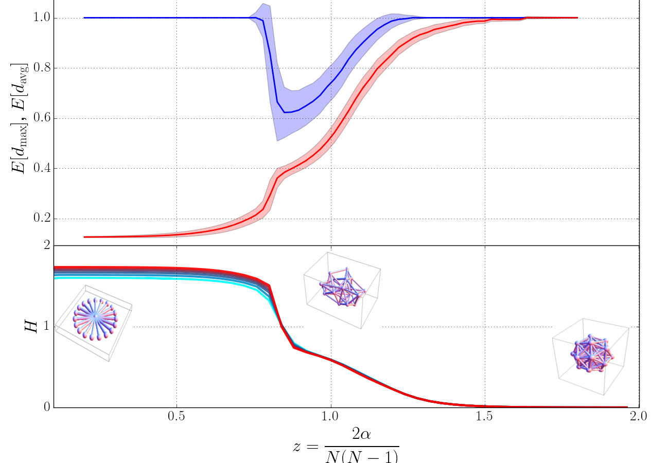
Figure 2: Top: Monte Carlo estimates of the maximum degree and the average degree ($I\kern-3.00003ptE(d_{avg})/(n-1)$ and $I\kern-3.00003ptE(d_{max})/(n-1)$) of the social web representation as a function of the specific cognitive capacity per dyadic relation $z=2\alpha/n(n-1)$ for $\beta=10$. The shaded areas are bands at $\pm 1$ std from the Monte Carlo. Bottom: $H=2(1-D)$, with $D=I\kern-3.00003ptE(d_{avg})/I\kern-3.00003ptE(d_{max})$. Roughly three regimes can be seen: for very large $z$, $H$ goes to zero (symmetric phase), all agents are equal. For very small $z$, $H$ is $\approx 2$, the broken symmetry phase, where a particular agent occupies the central position of the web. An intermediate $z$ transition region shows intermediate values of $H$. All agents are statistically but not strictly equals, some occupy, but only temporarily, in the stochastic dynamics a more central position. The different curves are for different values of $n(=10,11,...15)$ , note the almost exact colapse when plotted as a function of $z$. The insets are typical realizations of the inferred web of social interactions by an agent at that $z$ position. Bonds are only drawn if the bond variable is one.

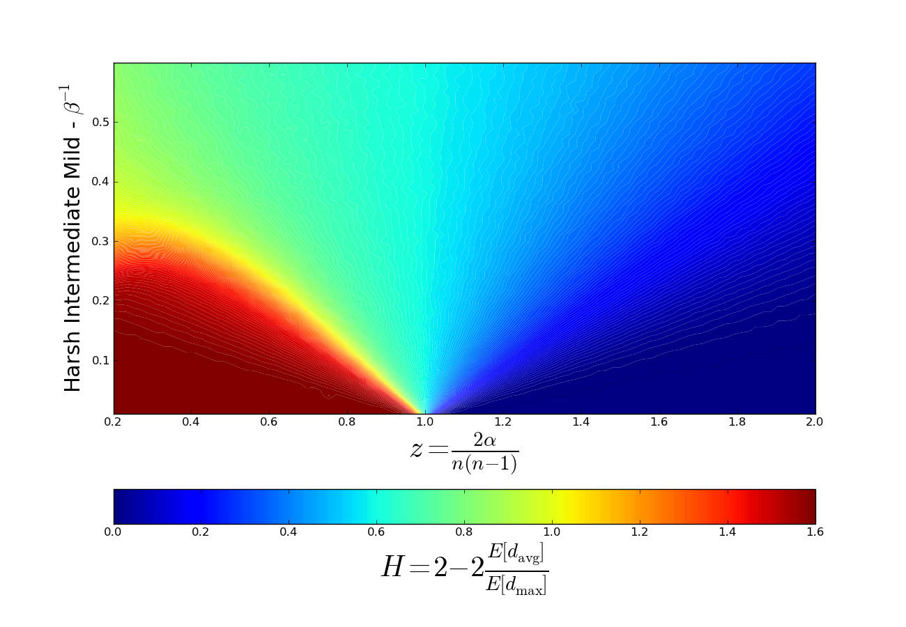
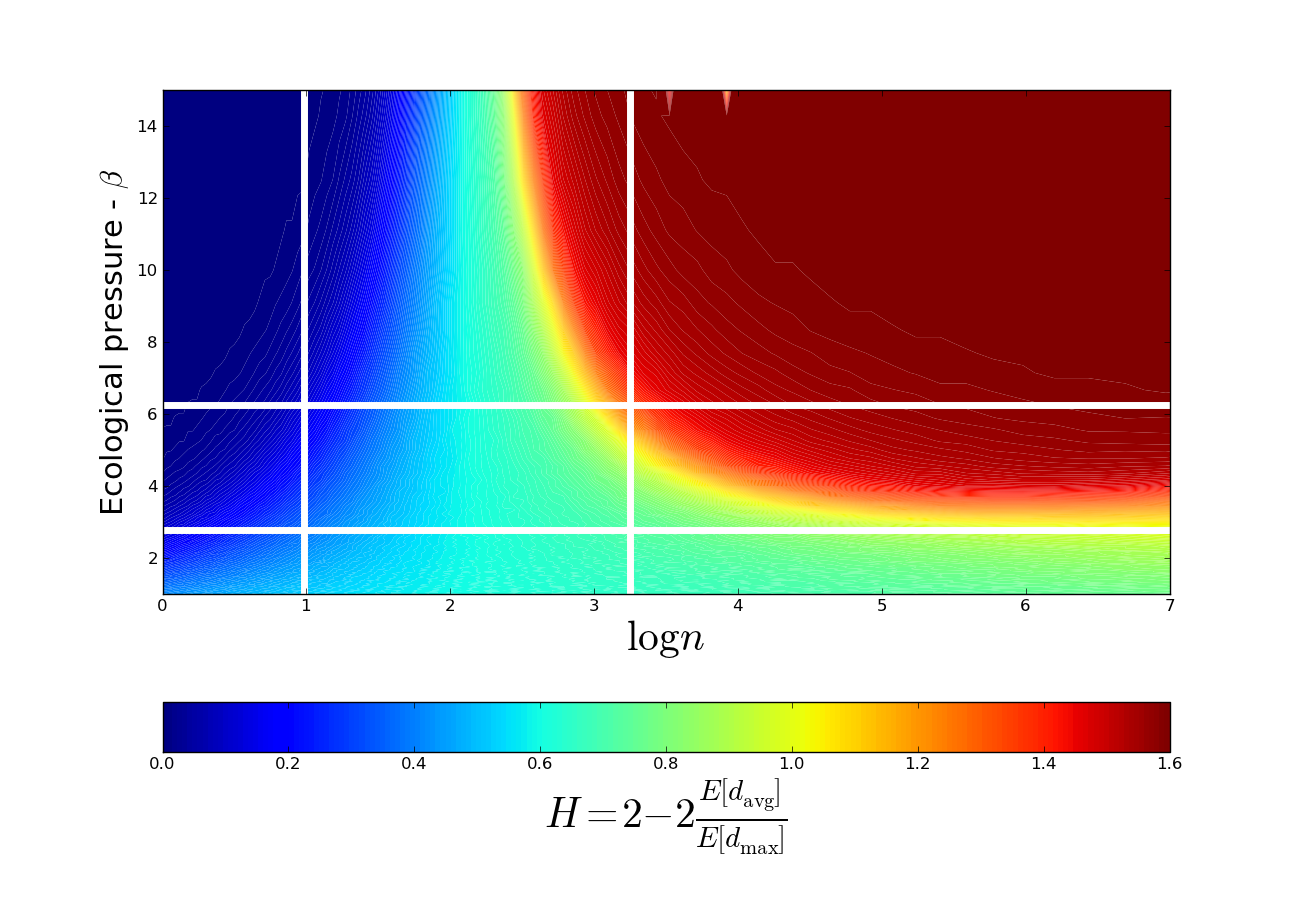
Figure 3: Left, Hierarchical-Egalitarian phase transition: phase diagram in the plane of specific cognitive capacity per dyadic relation $z=\frac{2\alpha}{n(n-1)}$ and the inverse ecological pressure $\beta^{-1}$. The color code represents a measure of the social hierarchy measure or symmetry breaking parameter $H=2-2I\kern-3.00003ptE(d_{avg})/I\kern-3.00003ptE(d_{max})$. The red region is where the symmetry is broken ($H$ near 2) and the maximum degree $I\kern-3.00003ptE(d_{max})$ is much larger than the mean $I\kern-3.00003ptE(d_{avg})$. The blue region is the unbroken symmetry phase, $H\approx 0$. Right, same but for constant $\alpha$ in the $\log n,\beta$ plane. The white lines divide the phase diagram into regions that can be used for the comparison to the Ethnographic Atlas data. The dark red region is where the symmetry is broken and the maximum degree is much larger than the mean. Dark blue is the symmetrical or egalitarian representation region.

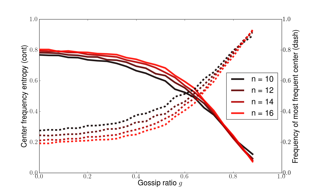
Figure 4: The effect of gossip inside the hierarchical phase. Continuous curves: The entropy (essentially a measure of the width (eq. 7)) of the distribution of central agents decreases with the increase of gossip, meaning that there is a particular agent that preferentially occupies the centers of the stars. Dashed lines: Another way of seeing the same ordering: the frequency of the most frequent central agent in their representations.

IV Results

IV.1 Joint dependence on cognition and band size

An interesting result is that, given $\beta$, to a good approximation the properties of the system do not depend separately on $\alpha$ and $n$ but on the ratio $z=\frac{2\alpha}{n(n-1)}$, which can be thought of as a measure of the effective cognitive capacity per dyadic relation on a social landscape.

We start by considering the case with no gossip $g=0$ where agents process information in a decoupled way. Larger $g$ gives similar results for the individual web representations but they are no longer independent and correlations of the webs appear. Figure 2 shows the results of Monte Carlo estimates of the order parameters, the expected values of $d_{max}$ and $d_{avg}$, respectively$I\kern-3.00003ptE(d_{avg})$ and $I\kern-3.00003ptE(d_{max})$. These are plotted as a function of the scaling variable $z=2\alpha/n(n-1)$. In the bottom of figure 2 we show the hierarchical order parameter $H=2-2D$ as a function $z$ for $\beta$ fixed, where $D=I\kern-3.00003ptE(d_{avg})/I\kern-3.00003ptE(d_{max})$. For $H=0$ the typical graph is the totally symmetric graph, while for $H=2$ the typical graph is the star. Since $n$ is finite, $H$ can’t be 2. The maximum value is $H_{max}=2(1-2/n+1/n^{2})\approx 2$. Three different regimes can be identified: low, intermediate and high $H$ regions. In figure 3 (left) we show $H$ as a heat map in the $z-\beta^{-1}$ plane. The three phases can be seen again. An intermediate fluid phase has the shape of a wedge that decreases in width as ecological pressure increases.

IV.2 Gossip and shared perception

Figure 4 shows how frequent is the most frequent central agent as a function of the level of gossip $g$. Let $P(c=j|i)$ be the probability that for the social web representation of agent $i$ the central element is $j$. The spreading of the probability distribution can be measured by the ratio of its entropy to the maximum possible value

$$s_{cf}=\frac{\bar{S}}{\log n}=\frac{-1}{n\log n}\sum_{i,j=1}^{n}P(c=j|i)\log P(c=j|i)$$ (7)

The results indicate that large correlation occurs when gossip dynamics dominates independent dynamics, starting around $g\approx 0.5$.

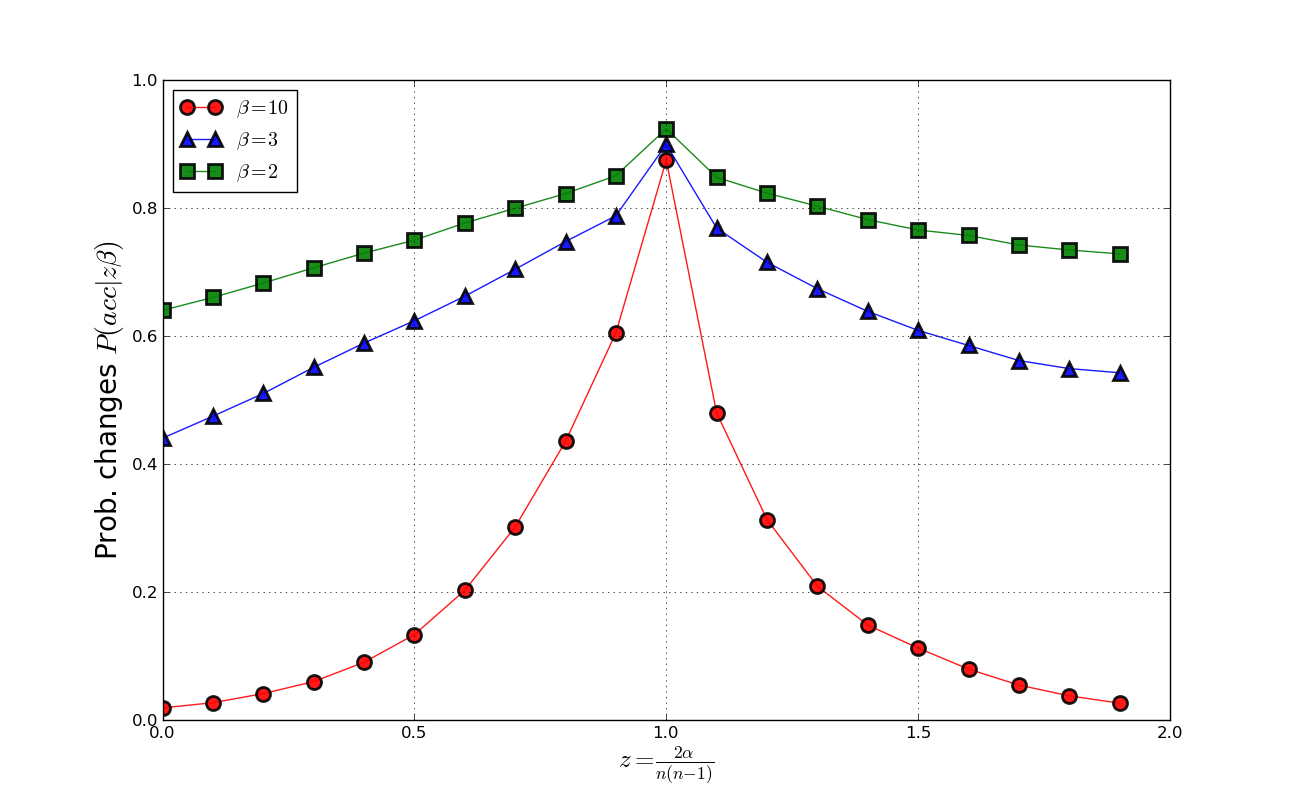
Figure 5: The probability of acceptance of changes $P(acc|z\beta)$ from the Monte Carlo simulations measures the tolerance to changes in the social web representations. As a function of $z$, for different values of $\beta$ ($\beta=2.,3.$ and $10$) For high pressure, or harsher environments, ($\beta=10$) changes that would permit upstarts to be different from other agents are not tolerated for large $z$. This is analogous to counter dominance behavior theory Boehm93 . Changes of the central agent of the star topology are unlikely to be accepted for small $z$. For milder pressures changes are more easily accepted. Tolerance is measured by the Monte Carlo acceptance probability

Again we stress the hypothesis that the likelihood of an agent in tolerating inequalities is associated to the perceived inequalities of its social web representation. The three regimes will have strong influence in the possibilities of social organization of the group. In the region where $H$ is close to zero, the interpretation is that no inequalities can be tolerated. These would represent large fluctuations on the cognitive-social cost and the combination of cognitive resources and band size given by $z$ is large enough to permit a representation web given by a full graph.

The intermediate wedge region could be interpreted as the “Big Man” society, where some inequality is possible, but is not solidified and these temporarily more central figures can be though of as “first among equals” and their position is liable to changes. Since the wedge decreases for increasing pressure, for extreme ecological pressure, a Big Man organization is not possible. Either there is a stable central figure, e.g. a chief, or symmetry among members of the band.

The lower left hand part of figure 3 (left) is where the symmetry breakdown of the web representation permits the emergence of tolerance towards inequalities. The exchange of information about the social webs leads to the choice of an almost unique and stable central agent for all agents. This would allow the creation of a society where authority is stable and social egalitarianism is lost. In figure 5 we show the probability of a change in the cognitive representation webs as a function of $z$, measured by the Monte Carlo (Metropolis) acceptance rate. Only in the intermediate Big Man fluid region a significant rate of changes is acceptable. In both hierarchical and egalitarian phases, the dynamics turns out to be very conservative and change is rare, maintaining status quo for very long times. This prediction of the theory is in accordance to what is expected from anthropology’s Reverse Dominance theory Boehm93 .

IV.3 Knauft’s U-shape

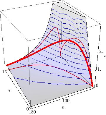
Figure 6: Schematic (inverted-) U-shape trajectory for the specific cognitive capacity $z\propto 2\alpha/n(n-1)$ as a function of time (thick curve). The higher the value of $z$, the more symmetrical or egalitarian the society will be. This is just a representation of externally caused changes in the cognitive capacity $\alpha(t)$ and the mean size of social groups $n(t)$ as a function of time. The thin lines are the shadows projected onto the respective planes. The surface is $z(\alpha,n)\propto\frac{2\alpha}{n(n-1)}$. The contours are drawn for constant $z$ values.

The fact that the phase diagram can be drawn using the combination $z=2\alpha/n(n-1)$ immediately suggests a scenario that accommodates the U-shape dynamics along the egalitarian-hierarchical spectrum. The schematic drawing in figure 6 shows the curve $z=z(\alpha(t),n(t))$ in a parametric representation using some rough measure of time as the parameter. We use a simple model of the growth of the cognitive capacity $\alpha$ in an evolutionary time scale and the fast increase in band sizes $n$ in the transition to the neolithic. For viewing purposes only we use different time scales along the trajectory so that the shape is clearly a nice inverted U, otherwise it would be very skewed, since it takes around 7 million years to go up from hierarchical to egalitarian and few thousands years to go down back to hierarchical. It starts with low $z$ around 7 Mya, in the hierarchical region of left hand side of the phase diagram of figure 3. It slowly grows, reaching a peak of $z$ in an egalitarian region due to increased encephalization. Finally it goes back to the region of low $z$ due to increase in band size, in the hierarchical phase of figure 3. Of course the specific details of such trajectory would depend on many other conditions, but this furnishes a plausible qualitative scenario for the evolution of $z$.

V Ethnographic data and theoretical predictions

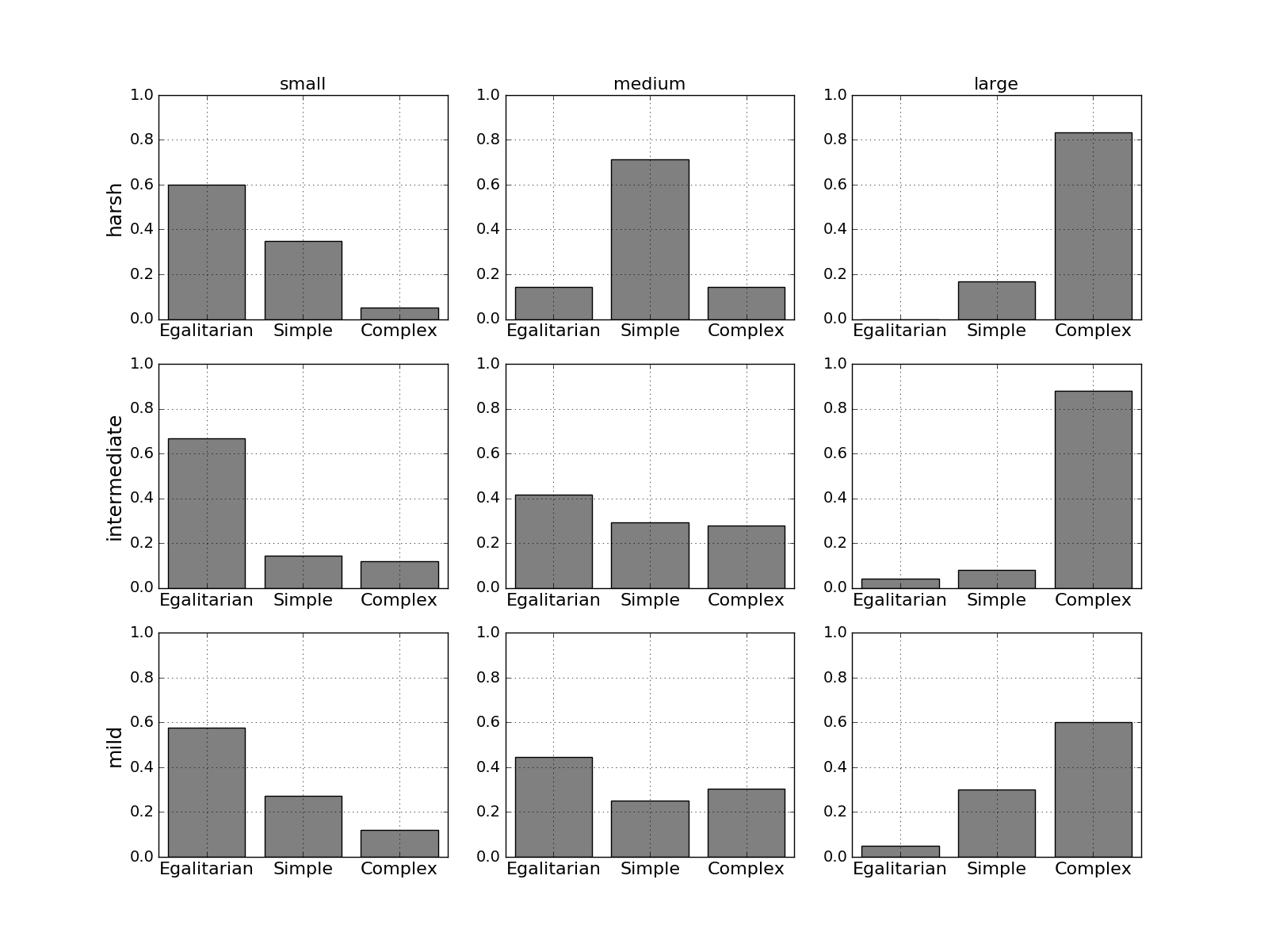
Figure 7:

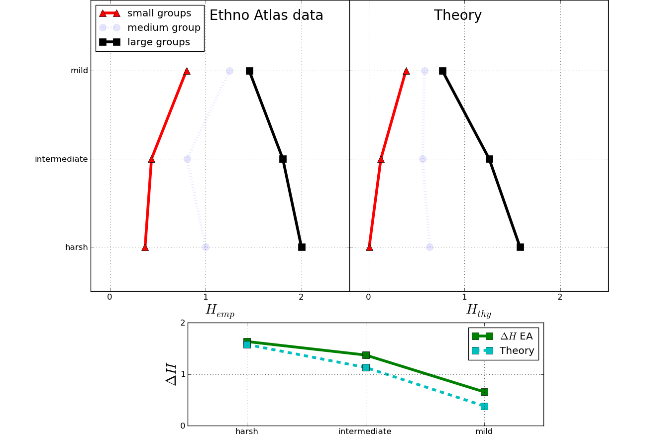
Figure 8: The bifurcation signature of the phase transition. For mild climates the expected hierarchies change little with group size. For harsh climates the expected hierarchy is larger for large groups and smaller for smaller groups. Top Left Ethnographic Atlas data. Top Right: theory. Bottom: The difference in expected hierarchy $\Delta H$ between large and small groups decreases for milder climates. Continuous line: EA data, Dashed line: theory. Harsh climates are Tundra (northern areas), Northern coniferous forest, High plateau steppe, Desert (including arctic). Mild: Temperate forest,Temperate grasslands, Mediterranean, Oases and certain restricted river valleys.

Can a signature of this competition between cognitive and social navigation constraints be seen today for modern humans? A clear theoretical prediction about the dependence of social stratification on ecological pressure $\beta$ and group size ($z=z(n)$, $\alpha$ fixed) can be confronted to data from the ethnographic record. The prediction is divided into two parts. First, for very mild climates intermediate social structures are expected, but, as climates of increasing harshness are considered, different social organizations will occur. Second, this difference depends on group size. Cultures organized in small groups will be more egalitarian, those in large groups more hierarchical.

Using Murdock’s Ethnographic Atlas (ethnoatlas ) we see in figure 8 that this prediction is indeed borne out by the data. These are not predictions about a specific group becoming more or less hierarchical as climate changes. These are predictions about the expectations we should have about hierarchical organization as different climates and group sizes are considered. Changes in a particular group would not be so easily observed, since the shift of perception of social webs will have an influence on motivations. See Wiessner2002 for a description of a system in the process of transition. How changing motivations lead to cultural changes and influence social organizations is outside the scope of the present theory.

From the Ethnographic Atlas we extracted the relevant variables: data for social stratification $h$, climate $c$ and group size $s$. Each variable range is divided into three regimes, low, intermediate and high ($0,1,2$ respectively, see SM ). The number of cultures in ethnoatlas with information on those three variables is 248. From the data we obtained the conditional probability $P(h|cs)=P(hcs)/P(cs)$. The empirical expected hierarchy value $H_{emp}=\sum_{h}hP(h|cs)$ for each possible combination of climate and size, is shown in the left panel of Figure 8. The climate variables describe the type of environment but we need a quantitative description of the climate instead of just its name. We decided that a reasonable conversion could be done by using the idea of Net Primary Production Ecology which is a measure of the amount of calories per day that can be extracted from the environment and therefore correlates negatively to the ecological pressure $\beta$.

To obtain the analogous theoretical predictions, the same is done by dividing the range of theoretical parameters into three intervals as well and calculating the same quantity from the theoretical results, see figure 3 (right). The theoretical expected value of $H_{thy}=2-2I\kern-3.00003ptE(d_{avg})/I\kern-3.00003ptE(d_{max})$ is shown in the right panel of Figure 8 .

The qualitative agreement between theory and empirical record supports that our methodology is capable of suggesting new ways of looking at the available ethnographic records, which can now come under scrutiny by the community of quantitative ethnography dealing with cross-cultural studies.

The fact that inequality rises with group size and that there are ecological factors involved, has been previously considered Carneiro ; Bingham99 ; Fletcher ; Summers2005 ; Dubreuilbook ; Keeley88 , but not how the rise is modulated by ecological pressure nor the hypothesis that this is due to the competition of cognitive and social navigation needs and therefore the influence of climatic pressure on hierarchy can be reversed by demographics. This papers are of a theoretical nature in the spirit of the social sciences. Mathematical attempts at modeling are typically absent and at most show the results of regressions between pairs of variables extracted from the ethnographic data.

VI Discussion

Our Statistical Mechanics approach, based on entropic inference through maximum entropy methods, is a methodological approach to the mathematical-physics modeling of systems that incorporates conditioning factors, in this case demographic, ecological, social and cognitive.

Our main hypothesis is that a social-cognitive cost is relevant to characterize probabilistically the perceived social webs. The introduction of the conjugated parameter $\beta$, with the same informational content of the average cost is an unavoidable theoretical consequence. It controls the size of fluctuations above the minimum possible value of the cost, prompting its interpretation as a pressure. Gossip, a metaphor for information exchange, correlates the perceived webs. The cognitive capacity and the size of the group combine into a variable $z$, the specific cognitive capacity, and the perceived social state can be described in a space of just two dimensions $(z,\beta)$. External to the model, the dynamics of encephalization and band size, determine the historical evolution of $z$ leading to a scenario for non-monotonic hierarchical change Knauft1991 . Further changes in $z$ could occur, e.g. due to technological advances which translate into more effective information processing and better social navigation. Also an effective reduction of ecological pressure, following enhanced productivity can occur. Then a more egalitarian perception of the social web will follow. The PMB hypothesis predicts that motivations and behaviors will change, but the theory does not go into the area of predicting how behaviors change, nor what institutions will emerge in order to permit such behaviors, nor the time scales of these changes. Our approach to the transition from hierarchical to egalitarian and back dispenses the issue of whether the hierarchical type of behavior lay dormant (Rodseth in Knauft1991 ) and remained present throughout the Pleistocene or whether the resurgence was due to convergent evolution (e.g. Smail2008 ). It can be turned on or off by the joint effects of cognitive resources, social demands, ecology and demography. These transitions resemble the freezing or evaporation of water by changing pressure or temperature. The possibility of being solid ice is not dormant in water when it is heated up. At least that is not a useful metaphor.

We can speculate that the time spent in the large $z$ egalitarian phase promoted conditions for the fixation of altruistic genes and the emergence of the ”do unto others” ideas since all are equal under the representation web. It is hard to imagine the fixation of altruistic behavior which arises from punishment and collaboration BoydRicherson ; BGB ; Schonmann2012 in other than the symmetric phase, but this should be amenable to model construction and analytic studies.

This simple model and the particular function we have used to represent the cognitive-social cost are far from complete. We don’t claim specific numerical validation by confrontation with empirical data, in any other way than just a qualitative one. More sophisticated forms of coalitions, other than dyadic pairing, should lead to increased richness of the phase diagram, without disrupting the rough overall picture. We have also avoided considering gender issues. Rampant sexual inequalities can exist in an egalitarian organization of males. Nevertheless, if competition between cognitive constraints and social navigation needs indeed occur, then phase transitions from egalitarian to hierarchical perception follows from general arguments. It has been argued Feinman that “in the history of the human species, there is no more significant transition than the emergence and institutionalization of inequality.” We expect that these methods, which unify the theoretical analysis of the empirical facts behind the scenario for the U-shape dynamics and the conditions that influence the transformation of perception of social organization, will stimulate the use of information theory methods in the analysis of empirical research in cross-cultural studies.

Acknowledgments: We thank Bruce Knauft for comments on a previous version of this paper and Helena L. Caticha for preparing Figure 1. This work was supported by Fapesp (2008/10830-2) and CNAIPS-USP.

Appendix A Appendix

A.1 Theory: Conditional Probabilities and order parameters

The phase diagram in the $\beta-z$ is shown right figure in panel 3. We divided the ranges of $\beta$ and $z$ into three regions each: harsh, intermediate and mild climates and small medium and large groups respectively. The phase diagram is thus divided into 9 regions. The regions are chosen essentially so that all points in the $\beta-z$ space in the harsh-large region are of the same color (blue). The same is done for the region of harsh-small (all red) and for mild-small and mild-large. The white lines show a reasonable choice of what is meant by large, intermediate and small both for $\beta$ and $n$. A reasonable choice for the values separating the three regions are $\beta^{-1}_{HI}=0.15$ and $\beta^{-1}_{IM}=0.35$. For $\beta^{-1}>\beta^{-1}_{IM}$, climate $c$ is mild. For $\beta^{-1}_{HI}<\beta^{-1}<\beta^{-1}_{IM}$, climate $c$ is intermediate, and $\beta^{-1}<\beta^{-1}_{HI}$, $c$ is harsh.

For $z=\frac{2\alpha}{n(n-1)}$ the borders are set at $z_{2}=0.6$ and $z_{1}=1.4$ For $2>z>z_{1}$, $s=1$ small. For $z_{2}>z>z_{1}$, $s=2$ intermediate. For $0<z<z_{2}$, $s=3$ large. Then we consider the order parameter $D(s,c)$

$$\bar{D}(s,c)=\frac{\int_{\beta\in c}\int_{z\in s}Ddzd\beta}{\int_{\beta\in c}\int_{z\in s}dzd\beta},$$ (8)

where $D=\frac{I\kern-2.10002ptE(d_{avg})}{I\kern-2.10002ptE(d_{max})}.$ and the theoretical hierarchical order parameter that can be compared to the data is $H_{thy}=2-2\bar{D}(s,c)$.

A.2 Data: Source

Data was obtained from ethnoatlas , the Ethnographic Atlas (EA) “a database on 1167 societies coded by George P. Murdock and published in 29 successive installments in the journal ETHNOLOGY, 1962-1980”, available for download from the site of Douglas R. White

http://eclectic.ss.uci.edu/ drwhite/worldcul/world.htm

We used the file EthnographicAtlasWCRevisedByWorldCultures.sav

The relevant variables for our study are $s$ , $h$ and $c$, which stand for size category, hierarchy category and climate category. All variables can take integer values $1$, $2$ or $3$. They are obtained by grouping the EA variables into three groups:

$\downarrow$Category, Value $\rightarrow$	1	2	3
s: group size (v31)	small	medium	large
h: social stratification (v66)	Egalitarian	Simple structure	Complex
c: Climate (v95)	Harsh	Intermediate	Mild

Table 1: EA variables and categories

		Number of cultures in	Number of cultures in	Number of cultures in
$\downarrow$Stratification	Climate	Small groups	Medium groups	Large groups
1	1	12	1	0
1	2	43	40	2
1	3	4	3	0
2	1	7	5	0
2	2	11	25	3
2	3	4	3	6
3	1	0	1	3
3	2	8	23	31
3	3	2	6	5

Table 2: Number of Cultures in the different categories in the EA.

A.3 Data: Conditional Probabilities and order parameters

This values are obtained by grouping the relevant variables of the EA according to tables 1-3SM below, into three categories. The results are presented in table 4SM below. We extract the numbers of cultures $N(s,h,c)$ with a given set of values $(s,h,c)$ and the marginal numbers $N(s,c)$ of cultures with a given pair of values of $(s,c)$ independently of $h$. These are related by $N(s,c)=\sum_{h=1,2,3}N(s,h,c)$. The conditional probabilities are

$$P(h|sc)=\frac{N(s,h,c)}{N(s,c)},$$ (9)

of a culture having a given class stratification , given its climate and group size.

Then we calculate the average hierarchy of the cultures with the same values of $n$ and $c$, that is, that belong to the same size and climate categories. We calculate the empirical average hierarchies conditional on size and climate

$$\bar{H}=I\kern-3.00003ptE(h-1|sc)=\sum_{h=1,2,3}(h-1)P(h|sc),$$ (10)

which satisfies $0\leq\bar{H}\leq 2$.

Fluctuations around the average

$$\sigma_{EA}^{2}=I\kern-3.00003ptE((h-\bar{h})^{2}|nc)=\sum_{h=1,2,3}(h-\bar{h})^{2}P(h|nc),$$ (11)

can be calculated to define error bars.

A.4 Numerical results

$\downarrow$Climate, Group size $\rightarrow$	Small	Medium	Large groups
Harsh	.37	1.	2.
Intermediate	.44	.81	1.81
Mild	.80	1.25	1.45

Table 3: The results for the empirical stratification $\bar{H}$

$\downarrow$Climate, Group size $\rightarrow$	Small	Medium	Large groups
Harsh	.01	.64	1.58
Intermediate	.13	.56	1.25
Mild	.39	.58	.77

Table 4: The results for the theoretical prediction $H_{T}$

A.5 Ethnographic data

N	Code	Description v31.	Size category
681	0	Missing data (code .)	0
118	1	Fewer than 50	1
107	2	50-99	1
104	3	100-199	2
83	4	200-399	2
60	5	400-1000	2
16	6	1,000 without any town of more than 5,000	3
36	7	Towns of 5,000-50,000 (one or more)	3
62	8	Cities of more than 50,000 (one or more)	3

Table 5: Variable v31 of the Ethnographic Atlas: Mean Size of Local Communities.

N	Code	Description v66.	Hierarchy category
182	0	Missing data (code .)	0
533	1	Absence among freemen (O.)	1
206	2	Wealth distinctions (W.)	2
39	3	Elite (based on control of land or other resources (E.)	2
228	4	Dual (hereditary aristocracy) (D.)	3
79	5	Complex (social classes) (C.)	3

Table 6: Variable v66 of the Ethnographic Atlas: Class Stratification.

N	Code	Description v95.	Climate category
869	0	Not coded	0
3	51	Desert (including arctic)	1
11	23	Tundra (northern areas)	1
21	36	Northern coniferous forest	1
8	44	High plateau steppe	1
5	65	Oases and certain restricted river valleys	1
37	52	Desert grasses and shrubs	2
16	56	Temperate woodland	2
24	74	Sub-tropical bush	2
27	78	Sub-tropical rain forest	2
64	84	Tropical grassland	2
14	87	Monsoon forest	2
113	88	Tropical rain forest	2
25	54	Temperate grasslands	3
19	46	Temperate forest (mostly mountainous)	3
11	55	Mediterranean (dry, deciduous, and evergreen forests)	3

Table 7: v95 Climate: Primary Environment. Group 1 is formed by NPP up to $350gC/m^{2}/year$ Group 2: between $350gC/m^{2}/year$ and $600gC/m^{2}/year$. Group 3: large than $600gC/m^{2}/year$.

A.6 Cultures: Size, Class Stratification , Climate

Table 8 List of all cultures with available information in all three categories

	Culture	Size(v31)	Stratification(v66)	Climate(v95)
1	!KUNG	1	1	2
2	ILA	2	2	2
3	NYORO	2	3	2
4	AMBA	2	1	2
5	KPE	1	2	2
6	FON	3	3	2
7	KISSI	2	1	2
8	BAMBARA	3	3	2
9	YATENGA	3	3	2
10	KATAB	2	1	2
11	KONSO	3	2	3
12	SOMALI	1	2	2
13	WOLOF	3	3	2
14	TEDA	1	3	3
15	BARABRA	1	2	1
16	GHEG	2	1	1
17	NEWENGLAN	3	3	2
18	DUTCH	3	3	2
19	SERBS	3	3	2
20	SYRIANS	3	2	3
21	SINDHI	3	2	2
22	KAZAK	1	3	3
23	GILYAK	1	1	1
24	YAKUT	1	2	1
25	KOREANS	3	3	2
26	LOLO	2	3	3
27	ABOR	2	2	2
28	CHENCHU	1	1	2
29	TAMIL	3	3	2
30	ANDAMANES	1	1	2
31	MERINA	3	3	2
32	GARO	2	2	2
33	LAMET	1	2	2
34	MNONGGAR	2	2	2
35	ATAYAL	2	1	2
36	SAGADA	3	2	2
37	JAVANESE	3	3	2
38	MACASSARE	2	3	2
39	ARANDA	1	1	2
40	KAPAUKU	1	2	2

	Culture	Size(v31)	Stratification(v66)	Climate(v95)
41	WANTOAT	1	1	2
42	TRUKESE	2	1	2
43	TROBRIAND	2	3	2
44	SAMOANS	1	3	2
45	TIKOPIA	2	3	2
46	NABESNA	1	1	1
47	TAREUMIUT	2	2	1
48	TWANA	1	2	1
49	NOMLAKI	2	2	3
50	TENINO	2	2	1
51	OJIBWA	1	1	1
52	HURON	2	2	1
53	HANO	2	1	2
54	CUNA	1	2	2
55	WARRAU	1	1	2
56	MUNDURUCU	1	1	2
57	SIRIONO	1	1	2
58	TUCUNA	2	1	2
59	INCA	3	3	1
60	YAHGAN	1	1	1
61	MATACO	1	1	2
62	TRUMAI	1	1	2
63	DOROBO	1	1	2
64	NAMA	2	2	2
65	LOZI	1	3	2
66	BEMBA	2	3	2
67	KUBA	2	3	2
68	CHAGGA	2	3	2
69	KIKUYU	2	2	2
70	FANG	1	2	2
71	ASHANTI	3	3	2
72	DOGON	2	2	2
73	TALLENSI	2	2	2
74	TIV	2	1	2
75	AZANDE	2	3	2
76	MASAI	1	1	2
77	TIGRINYA	3	3	2
78	SONGHAI	3	3	2
79	SIWANS	3	2	3
80	EGYPTIANS	3	3	3

	Culture	Size(v31)	Stratification(v66)	Climate(v95)
81	RIFFIANS	3	2	3
82	ROMANS	3	3	3
83	IRISH	3	3	2
84	LAPPS	1	2	1
85	HUTSUL	3	2	3
86	PATHAN	2	3	2
87	KHALKA	1	3	2
88	CHUKCHEE	1	2	1
89	YURAK	1	2	1
90	MIAO	2	1	2
91	BURUSHO	2	3	1
92	LEPCHA	2	2	3
93	BENGALI	3	3	2
94	MARIAGOND	1	2	2
95	TODA	1	1	2
96	TANALA	2	3	2
97	VEDDA	1	1	2
98	BURMESE	3	3	2
99	SEMANG	1	1	2
100	ANNAMESE	3	3	2
101	IFUGAO	2	2	2
102	SUBANUN	1	1	2
103	BALINESE	2	3	2
104	ALORESE	2	2	2
105	MURNGIN	1	1	2
106	TIWI	2	1	2
107	WOGEO	1	1	2
108	MAJURO	2	3	2
109	IFALUK	1	1	2
110	KURTATCHI	2	3	2
111	LESU	2	1	2
112	BUNLAP	1	2	2
113	LAU	1	2	2
114	PUKAPUKAN	2	1	2
115	MAORI	2	3	3
116	MARQUESAN	1	3	2
117	COPPERESK	1	1	1
118	KASKA	1	1	1
119	YUROK	1	2	3
120	TUBATULAB	1	1	2

	Culture	Size(v31)	Stratification(v66)	Climate(v95)
121	HAVASUPAI	2	1	2
122	SANPOIL	1	1	3
123	OMAHA	1	1	3
124	CREEK	2	1	3
125	NAVAHO	2	1	2
126	ZUNI	3	1	2
127	AZTEC	3	3	3
128	BARAMACAR	1	1	2
129	TAPIRAPE	2	1	2
130	JIVARO	1	1	1
131	YAGUA	1	1	2
132	AYMARA	2	2	1
133	CAYAPA	2	1	2
134	MAPUCHE	1	2	3
135	BACAIRI	1	1	2
136	NAMBICUAR	1	1	2
137	AWEIKOMA	1	1	2
138	RAMCOCAME	2	1	2
139	MBUTI	2	1	2
140	MBUNDU	2	3	2
141	VENDA	2	3	3
142	NYAKYUSA	2	1	2
143	MENDE	2	3	2
144	YORUBA	3	3	2
145	BIRIFOR	2	1	2
146	MAMBILA	2	1	3
147	MARGI	2	1	2
148	MAMVU	1	1	2
149	SHILLUK	2	3	2
150	LANGO	2	2	2
151	IRAQW	2	2	2
152	MZAB	3	3	3
153	KABYLE	2	1	2
154	TRISTAN	2	1	3
155	WALLOONS	3	3	2
156	CZECHS	3	3	2
157	HEBREWS	3	3	3
158	HAZARA	2	2	2
159	KORYAK	2	2	1
160	YUKAGHIR	1	1	1

	Culture	Size(v31)	Stratification(v66)	Climate(v95)
161	JAPANESE	3	3	2
162	MINCHINES	3	3	2
163	TIBETANS	3	3	1
164	COORG	2	3	2
165	KERALA	3	3	2
166	NICOBARES	1	1	2
167	SINHALESE	3	3	2
168	KACHIN	2	3	3
169	PURUM	1	2	2
170	CAMBODIAN	3	3	2
171	HANUNOO	2	1	2
172	DUSUN	2	2	2
173	DIERI	1	1	2
174	KARIERA	1	1	2
175	KERAKI	1	1	2
176	PONAPEANS	1	3	2
177	YAPESE	1	3	2
178	ULAWANS	2	1	2
179	NASKAPI	1	1	1
180	EYAK	1	2	1
181	ATSUGEWI	1	2	3
182	MIAMI	2	1	2
183	CHEROKEE	2	1	2
184	DELAWARE	2	1	2
185	MARICOPA	1	1	2
186	TAOS	2	1	2
187	HUICHOL	2	2	2
188	CHOCO	1	1	2
189	CARINYA	2	1	2
190	GUAHIBO	1	1	2
191	CUBEO	1	1	2
192	TUNEBO	2	1	2
193	ONA	1	1	1
194	CHOROTI	1	1	2
195	CAMAYURA	2	1	2
196	BOTOCUDO	1	1	2
197	SOTHO	2	3	3
198	YAO	2	1	2
199	YOMBE	2	3	2
200	GANDA	3	3	2

	Culture	Size(v31)	Stratification(v66)	Climate(v95)
201	BETE	2	1	2
202	NUPE	2	3	2
203	CONIAGUI	1	1	2
204	BAYA	2	1	2
205	LUO	2	2	2
206	CHEREMIS	2	2	2
207	NURI	2	2	2
208	AINU	1	1	2
209	OKINAWANS	3	3	2
210	DARD	2	3	2
211	BHIL	1	3	2
212	AKHA	2	1	2
213	PAIWAN	2	3	2
214	WIKMUNKAN	1	1	2
215	ENGA	2	1	2
216	LAKALAI	2	2	2
217	ATTAWAPIS	1	1	1
218	DIEGUENO	2	1	2
219	WASHO	1	1	3
220	PAWNEE	2	3	3
221	COCHITI	2	1	2
222	YUCATECMA	3	3	2
223	WAICA	1	1	2
224	TEHUELCHE	1	1	2
225	NGONI	2	3	2
226	WUTE	2	3	2
227	BRAZILIAN	3	3	2
228	BULGARIAN	3	3	2
229	BASSERI	2	2	2
230	KET	1	1	1
231	MINCHIA	2	2	3
232	KHASI	1	3	2
233	SIAMESE	3	2	2
234	PURARI	2	2	2
235	ONOTOA	2	2	2
236	MANUS	2	2	2
237	YUKI	1	2	3
238	NATCHEZ	2	2	2
239	JEMEZ	2	1	2
240	BLACKCARI	3	1	2
241	MAM	3	2	3
242	MISKITO	2	1	2
243	GOAJIRO	1	2	2
244	YABARANA	1	1	2
245	CHIBCHA	3	3	1
246	ALACALUF	1	1	3
247	APINAYE	1	1	2
248	TUPINAMBA	2	2	2

References

- (1) Bruce M. Knauft, Thomas S. Abler, Laura Betzig, Christopher Boehm, Robert Knox Dentan, Thomas M. Kiefer, Keith F. Otterbein, Tohn Paddock, and Lars Rodseth. Violence and sociality in human evolution [and comments and replies]. Current Anthropology, 32:391–428, 1991.
- (2) Christopher Boehm. Hierarchy in the Forest: The Evolution of Egalitarian Behavior. Harvard University Press, 1999.
- (3) Christopher Boehm. Ancestral hierarchy and conflict. Science, 336:844–847, 2012.
- (4) Benoit Dubreuil. Paleolithic public goods games: why human culture and cooperation did not evolve in one step. Biol Philos, 25:53–73, 2010.
- (5) Benoit Dubreuil. Human Evolution and the Origins of Hierarchies. Cambridge: Cambridge University Press, 2010.
- (6) SL Vehrencamp. A model for the evolution of despotic versus egalitarian societies. Animal Behaviour, 31:667–682, 1983.
- (7) Satoru Yamadera and Takao Terano. Examining the myth of money with agent-based modelling. In B. Edmonds, K. Troitzsch, and C. Hernández Iglesias, editors, Social Simulation: Technologies, Advances and New Discoveries, pages 252–263. Hershey, PA: Information Science Reference, 2008.
- (8) Masaaki Kunigami, Masato Kobayashi, Satoru Yamadera, and Takao Terano. On emergence of money in self-organizing doubly structural network model. In Takao Terano, Hajime Kita, Shingo Takahashi, and Hiroshi Deguchi, editors, Agent-Based Approaches in Economic and Social Complex Systems V, volume 6 of Springer Series on Agent Based Social Systems, pages 231–241. Springer Japan, 2009.
- (9) G. P. Murdock. Ethnographic atlas. University of Pittsburgh Press, Pittsburgh, PA, 1967.
- (10) George P Murdock and Douglas R. White. Standard cross-cultural sample: on-line edition. social dynamics and complexity. uc irvine: Social dynamics and complexity. Ethnology, http://escholarship.org/uc/item/62c5c02n, pages 329–269, 1969.
- (11) Ariel Caticha. Lectures on probability, entropy and statistical physics. arxiv:0808.0012 [physics.data-an].
- (12) C. Boehm. Egalitarian society and reverse dominance hierarchy. Current Anthropology, 34:227–254, 1993.
- (13) Polly Wiessner. The vines of complexity. Current Anthropology, 43(2):233–269, 2002.
- (14) Supplementary material.
- (15) R H Whittaker and P Stilling. Ecology: Theory and Applications. Prentice-Hall, 1996.
- (16) Robert L. Carneiro. On the relationship between size of population and complexity of social organization. Southwestern Journal Anthropology, 23:2–43, 1967.
- (17) P. Bingham. Human uniqueness: a general theory. Quarterly Review of Biology, 74:133–169, 1999.
- (18) Roland Fletcher. The Limits of Settlement Growth: A theoretical outline. Cambridge: Cambridge University Press, 2007.
- (19) Kyle Summers. The evolutionary ecology of despotism. Evolution and Human Behavior, 26(1):106–135, January 2005.
- (20) Lawrence H. Keeley. Hunter-gatherer economic complexity and “population pressure”: A cross-cultural analysis. Journal of Anthropological Archaeology, 7:373–411, 1988.
- (21) Daniel L Smail. On Deep History and the Brain. University of California Press, 2008.
- (22) R. Boyd and P. J. Richerson. The evolution of reciprocity in sizable groups. J Theor Biol, 132:337–356, 1988.
- (23) Robert Boyd, Herbert Gintis, and Samuel Bowles. Coordinated punishment of defectors sustains cooperation and can proliferate when rare. Science, 328:617–620, 2010.
- (24) Roberto H. Schonmann, Renato Vicente, and Nestor Caticha. Altruism can proliferate through population viscosity despite high random gene flow. PLoS ONE, 8(8):e72043, 08 2013.
- (25) G. M. Feinman. The emergence of inequality. In T. Douglas Price and G. M. Feinman, editors, Foundations of social inequality, pages 255–279. Plenum Press, 1995.