Universal scaling of Néel temperature, staggered magnetization density, and spinwave velocity of three-dimensional disordered and clean quantum antiferromagnets

Abstract

The Néel temperature, staggered magnetization density, as well as the spinwave velocity of a three-dimensional (3D) quantum Heisenberg model with antiferromagnetic disorder (randomness) are calculated using first principles non-perturbative quantum Monte Carlo simulations. In particular, we examine the validity of universal scaling relations that are related to these three studied physical quantities. These relations are relevant to experimental data and are firmly established for clean (regular) 3D dimerized spin-1/2 Heisenberg models. Remarkably, our numerical results show that the considered scaling relations remain true for the investigated model with the introduced disorder. In addition, while the presence of disorder may change the physical properties of regular dimerized models, hence leading to different critical theories, both the obtained data of Néel temperature and staggered magnetization density in our study are fully compatible with the expected critical behaviour for clean dimerized systems. As a result, it is persuasive to conclude that the related quantum phase transitions of the considered disordered model and its clean analogues are governed by the same critical theory, which is not always the case in general. Finally, we also find smooth scaling curves even emerging when both the data of the investigated disordered model as well as its associated clean system are taken into account concurrently. This in turn implies that, while in a restricted sense, the considered scaling relations for 3D spin-1/2 antiferromagnets are indeed universal.

I Introduction

Universality is an elegant concept and frequently appears in all fields of physics in various forms. In addition to being important in theoretical physics, the idea of universality can also serve as useful guidelines for experiments. One well-known example of the usefulness of universality is the critical exponents of second order phase transitions Nig92 ; Sac99 ; Car10 . Specifically, the numerical values of critical exponents, such as $\nu$ related to the correlation length and $\beta$ associated with the magnetization, do not in principle depend on the microscopic details of the underlying models, but are closely connected to the symmetries of the considered systems. For example, the zero temperature phase transitions of two-dimensional (2D) dimerized quantum Heisenberg models are governed by the $O(3)$ universality class Mat02 ; Wan05 ; Wen08 ; Alb08 ; Wen09 ; Jia09 ; Jia12 , which is originally resulted from the three-dimensional (3D) classical Heisenberg model Cam02 ; Pel02 . Furthermore, the spatial dimerization patterns have no impact on the critical theories of these quantum phase transitions (However, there may be anomolous corrections to scalings Wen08 ; Fri11 ; Jia12 ). Another noticeable kind (and example) of universality is the generally applicable finite-temperature and -volume expressions of several physical quantities of antiferromagnets Cha88 ; Reg88 ; Cha89 ; Neu89 ; Has90 ; Has91 ; Has93 ; Chu94 ; Wie94 ; Tro95 ; Bea96 ; San97 ; Jia08 ; Jia09.1 ; Jia11.1 . To be more precise, based on the corresponding low-energy effective field theory, the theoretical predictions of these observables, such as staggered and uniform susceptibilities, depend solely on a few parameters and have the same forms regardless of the magnitude of the spin of the systems. In conclusion, universality does play a crucial role in major areas of physics.

Recently, the experimental data of the phase diagram of TlCuCl₃ under pressure Cav01 ; Rue03 ; Rue08 have triggered many studies both theoretically and experimentally. In particular, several universal scaling relations are established for 3D quantum antiferromagnets Kul11 ; Oit12 ; Jin12 ; Kao13 ; Mer14 . Specifically, near the quantum phase transitions of clean (regular) 3D dimerized spin-1/2 Heisenberg models, the Néel temperatures $T_{N}$ scale in several universal manners with the corresponding staggered magnetization density $M_{s}$ regardless of the dimerization patterns. In addition, a quantum Monte Carlo study conducted later demonstrates that these universal scaling relations even remain valid when (certain kinds of) quenched bond disorder, i.e. antiferromagnetic bond randomness are introduced into the systems Tan15 . Notice the upper critical spatial dimension of the mentioned zero-temperature phase transitions is three. Consequently, close to the critical points one expects to observe multiplicative logarithmic corrections to $T_{N}$ and $M_{s}$ when these quantities are considered as functions of the strength of dimerization. Very recently an analytic investigation even argues that the widely believed phase diagram of 3D quantum antiferromagnets is modified dramatically due to these logarithmic corrections Har16 . The exponents related to these logarithmic corrections are determined analytically in Refs. Ken04 ; Ken12 ; Har15 ; Yan15 . Furthermore, the theoretical predictions of the numerical values of these new exponents have been verified as well Yan15 . Notice that the exponents related to the logarithmic corrections to $T_{N}$ and $M_{s}$ take the same values for three spatial dimenions. Using this result as well as the fact that the $\beta$ and $\nu$ have the same mean-field values, it is straightforward to show that close the the phase transition, as functions of their corresponding $M_{s}$, $T_{N}/c^{3/2}$ and $T_{N}/\overline{J}$ are linear in $M_{s}$ without any logarithmic corrections. Here $c$ and $\overline{J}$ are the low-energy constant spinwave velocity and the average of antiferromagnetic couplings, respectively. These connections between $T_{N}$ and the associated $M_{s}$, namely $T_{N}/c^{3/2}=AM_{s}$ and $T_{N}/\overline{J}=A_{1}M_{s}$ ($A$ and $A_{1}$ are some constants) in the vicinity of a quantum critical point are confirmed in Ref. Yan15 . In real materials, impurities are often present Vaj02 . In addition, studies of quenched disorder effects on Heisenberg-type models continue to be one of the active research topics in condensed matter physics Voj10 . Therefore one intriguing physics to explore further is that whether the logarithmic corrections, as well as the linear dependence of $T_{N}/c^{3/2}$ and $T_{N}/\overline{J}$ on their associated $M_{s}$ are valid for 3D systems with the presence of antiferromagnetic bond disorder. Since such studies of disordered models are relevant to the experimental data of TlCuCl₃, in this investigation we have carried out a large-scale quantum Monte Carlo simulations of a 3D spin-1/2 antiferromagnet with configurational disorder which is first introduced in Ref. Yao10 . Remarkably, our data indicate convincingly that for the studied disordered model, $\overline{T_{N}}/\overline{c}^{3/2}$ and $\overline{T_{N}}/\overline{J}$ do depend on their corresponding $\overline{M_{s}}$ linearly close to the associated quantum phase transition (In this study observables with a overline on them refer to the results of disorder average). Furthermore, the obtained data of $\overline{T_{N}}$ and $\overline{M_{s}}$ here can be described well by the expected critical behaviour for regular dimerized models. This suggests that the related quantum phase transition of the considered disordered system may be governed by the same critical theory as that of its clean analogues. It should be pointed out that while close to the considered quantum critical point the relations $\overline{T_{N}}/\overline{c}^{3/2}=A\overline{M_{s}}$ and $\overline{T_{N}}/\overline{J}=A_{1}\overline{M_{s}}$ hold even for the investigated model with the employed disorder, based on the results of current and previous studies, we find that the prefactor $A$ and $A_{1}$ are likely to be model-dependent. Surprisingly, when both the data of current study and that of a clean system available in Ref. Kao13 are taken into account concurrently, smooth universal curves appear. This in turn implies that, while in a restricted sense, the investigated scaling relations of 3D spin-1/2 antiferromagnets are indeed universal. Finally, although the prefactor $A$ of $T_{N}/c^{3/2}=AM_{s}$ ($\overline{T_{N}}/\overline{c}^{3/2}=A\overline{M_{s}}$) is likely not universal, we find the quantity $A/(J^{\prime}/J)_{c}^{3/2}$, where $(J^{\prime}/J)_{c}$ is the considered critical point, obtained in this study matching very well with the corresponding one in Ref. Yan15 . This indicates that with an appropriate normalization, a true universal quantity may still exist.

This paper is organized as follows. After the introduction, in section 2 we define the investigated model as well as the calculated observables. We then present a detail analysis of our numerical data in section 3. In particular, the scaling relation $T_{N}/c^{3/2}=AM_{s}$ as well as the logarithmic corrections to $T_{N}$ and $M_{s}$ are examined carefully. Finally in section 4 we conclude our study.

II Microscopic model, configurational disorder, and observables

The 3D quantum Heisenberg model with random antiferromagnetic couplings studied here is given by the Hamilton operators

$$H=\sum_{\langle ij\rangle}J_{ij}\,\vec{S}_{i}\cdot\vec{S}_{j}+\sum_{\langle i^{\prime}j^{\prime}\rangle}J^{\prime}_{i^{\prime}j^{\prime}}\,\vec{S}_{i}\cdot\vec{S}_{j},$$ (1)

where $J_{ij}$ and $J^{\prime}_{i^{\prime}j^{\prime}}$ are the antiferromagnetic couplings (bonds) connecting nearest neighbor spins $\langle ij\rangle$ and $\langle i^{\prime}j^{\prime}\rangle$, respectively, and $\vec{S}_{i}$ is the spin-1/2 operator at site $i$. The bond disorder considered in this investigation is a generalization of the configurational disorder introduced in Ref. Yao10 and is realized here as follows. First of all, a given cubical lattice is subdivided into two by two by two cubes. Secondly, the 12 bonds within a cube is classified into three sets of bonds so that each of them is made up of four bonds parallel to a particular coordinate axis. Furthermore, one of the three sets of bonds of every cube is chosen randomly and uniformly. In particular, these picked bonds are assigned the antiferromagnetic coupling strength $J^{\prime}$. Finally the remaining unchosen bonds as well as those not within any cubes have antiferromagnetic coupling strength $J$ which is set to be $1.0$ in this investigation. Figure 1 demonstrates one realization of the model with configurational disorder studied here. Notice in our study the couplings $J^{\prime}$ and $J$ satisfy $J^{\prime}>J$. Hence as the ratio of $J^{\prime}/J$ increases, the system will undergoes a quantum phase transition.

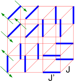
Figure 1: The model with configurational disorder studied here.

To determine the Néel temperature $\overline{T_{N}}$, the staggered magnetization density $\overline{M_{s}}$, as well as the spinwave velocity $\overline{c}$ of the considered models with the employed configurational disorder, the observables staggered structure factor $\overline{S(\pi,\pi)}$, both the spatial and temporal winding numbers squared ($\overline{\langle W_{i}^{2}\rangle}$ for $i\in\{1,2,3\}$ and $\overline{\langle W_{t}^{2}\rangle}$), spin stiffness $\overline{\rho_{s}}$, first Binder ratio $\overline{Q_{1}}$, and second Binder ratio $\overline{Q_{2}}$ are calculated in our simulations. The quantity $\overline{S(\pi,\pi)}$ takes the form

$$\overline{S(\pi,\pi)}=3\overline{\langle(m_{s}^{z})^{2}\rangle}$$ (2)

on a finite cubical lattice with linear size $L$. Here $m_{s}^{z}=\frac{1}{L^{3}}\sum_{i}(-1)^{i_{1}+i_{2}+i_{3}}S^{z}_{i}$ with $S^{z}_{i}$ being the third-component of the spin-1/2 operator $\vec{S}_{i}$ at site $i$. In addition, the spin stiffness $\overline{\rho_{s}}$ has the following expression

$$\overline{\rho_{s}}=\frac{1}{3\beta L}\sum_{i=1,2,3}\overline{\langle W_{i}^{2}\rangle},$$ (3)

where $\beta$ is the inverse temperature. Finally the observables $\overline{Q_{1}}$ and $\overline{Q_{2}}$ are defined by

$$\overline{Q_{1}}=\frac{\overline{\langle|m_{s}^{z}|\rangle}^{2}}{\overline{\langle(m_{s}^{z})^{2}\rangle}}$$ (4)

and

$$\overline{Q_{2}}=\frac{\overline{\langle(m_{s}^{z})^{2}\rangle}^{2}}{\overline{\langle(m_{s}^{z})^{4}\rangle}},$$ (5)

respectively. With these observables, the physical quantities required for our study, namely $\overline{T_{N}}$, $\overline{M_{s}}$, and $\overline{c}$, can be calculated accurately.

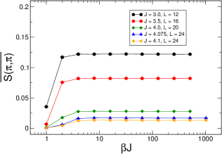
Figure 2: Convergence of the structure factors $\overline{S(\pi,\pi)}$ to their ground state values for several considered $J^{\prime}/J$ and box sizes $L$. The solid lines are added to guide the eye.

III The numerical results

To examine whether the scaling relations $\overline{T_{N}}/\overline{c}^{3/2}=A\overline{M_{s}}$ and $\overline{T_{N}}/\overline{J}=A_{1}\overline{M_{s}}$, where $A$ and $A_{1}$ are some constant, appear for the considered 3D quantum Heisenberg models with the introduced configurational disorder, we have carried out a large-scale Monte Carlo simulation using the stochastic series expansion (SSE) algorithm with very efficient loop-operator update San99 . We also use the $\beta$-doubling scheme San02 in our simulations so that $\overline{M_{s}}$ can be obtained efficiently. Here $\beta$ refers to the inverse temperature. Furthermore, each disordered configuration is generated by its own random seed in order to reduce the effect of correlation between observables determined from different configurations. Our preliminary results indicate that the critical point $(J^{\prime}/J)_{c}$ lies between 4.15 and 4.17. Hence we have focused on the data of $J^{\prime}/J\leq 4.13$. Notice in our study, $\overline{M_{s}}$ are calculated using several hundred configurations and $\overline{T_{N}}$ ($\overline{c}$) are determined with several thousand (few to several ten thousand) disorder realizations. The convergence of the considered observables to their correct values associated with the employed disorder, as well as the systematic uncertainties due to Monte Carlo sweeps within each randomness realization, number of configurations used for disorder average, and thermalization are examined by performing many trial simulations and analysis. The resulting data from these trial simulations and analysis agree quantitatively with those presented here. Notice the statistics reached for studies of clean systems typically is better than that of investigation related to disordered models. Therefore, we have additionally carried out many calculations using exactly the same parameters to estimate the uncertainties due to the statistics obtained here. In summary, the quoted errors of the calculated observables in this study are estimated with conservation so that the influence of these mentioned potential systematic uncertainties are not underestimated.

III.1 The determination of $\overline{M_{s}}$

The observable considered here for the calculations of $\overline{M_{s}}$ is $\overline{S(\pi,\pi)}$. Specifically, for a given $J^{\prime}/J$, the related $\overline{M_{s}}$ is given by the square root of the corresponding bulk $\overline{S(\pi,\pi)}$. It should be pointed out that the zero temperature, namely the ground state values of $\overline{S(\pi,\pi)}$ are needed for these calculations. Hence the $\beta$-doubling scheme is used here. The $\beta$-dependence, i.e. inverse temperature-dependence of $\overline{S(\pi,\pi)}$ for several considered $J^{\prime}/J$ and $L$ is shown in fig. 2. In addition, the $1/L$-dependence of the ground state $\overline{S(\pi,\pi)}$ for some studied $J^{\prime}/J$ is depicted in fig. 3. The largest box size reached here for calculating the staggered structure factors is $L=36$. Motivated by the theoretical predictions in Ref. Car96 , the determination of $\overline{M_{s}}$ is done by extrapolating the related finite volume staggered structure factors to the corresponding bulk results, using the following four ansatzes

$$a_{0}+a_{1}/L+a_{2}/L^{2}+a_{3}/L^{3},$$ (6)

$$b_{0}+b_{1}/L+b_{2}/L^{2},$$ (7)

$$c_{0}+c_{2}/L^{2}+c_{3}/L^{3},$$ (8)

$$d_{0}+d_{2}/L^{2}.$$ (9)

In particular, $\overline{M_{s}}$ are obtained by taking the square root of the resulting constant terms of the fits. Figure 4 shows the numerical values of $\overline{M_{s}}$ which are determined from the fits employing ansatz (7) and are used for the required analysis in this investigation. Furthermore, we also make sure that the presented results in fig. 4 are convergent with respect to the elimination of more smaller box size data in the fits, and are consistent with the stablized values obtained from applying ansatzes (6), (8), and (or) (9) to fit the data.

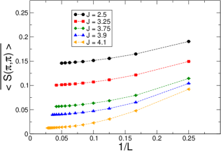
Figure 3: $1/L$-dependence of the staggered structure factors $\overline{S(\pi,\pi)}$ for several considered values of $J^{\prime}/J$. The dashed lines are added to guide the eye.

In Ref. Yan15 , the 3D dimerized double cubic quantum Heisenberg model is studied. In particular, the relation of $T_{N}/c^{3/2}=AM_{s}$ is examined in detail. Since three spatial dimensions is the upper critical dimension of the quantum phase transition considered in Ref. Yan15 , one expects to observe logarithmic corrections to $M_{s}$ and $T_{N}$ when approaching the critical point. The theoretical calculations of the critical exponents associated with these logarithmic corrections are available in Refs. Ken04 ; Ken12 ; Yan15 , and the predicted values are confirmed by a careful analysis of $M_{s}$ and $T_{N}$ conducted in Ref. Yan15 . Since disorder may change the upper critical dimension of the clean system, it will be interesting to check whether this is indeed the case for our model. The exponent related to the logarithmic correction to $M_{s}$, namely $\hat{\beta}$ has a value of $\frac{3}{11}$ for 3D clean dimerized model. Inspired by this, we have fitted our $\overline{M_{s}}$ data to an ansatz of the form

$$a|j_{c}-j|^{b}|\ln(|(j_{c}-j)/j_{c}|)|^{3/11},$$ (10)

where $j=J^{\prime}/J$ ($j_{c}=(J^{\prime}/J)_{c}$ is the critical point) and $a$ is a constant. Notice the $b$ appearing in Eq. (10) is the associated leading critical exponent which is predicted to be 0.5. Interestingly, we find that the numerical values of $b$ (in Eq. (10)) obtained from the fits have an average of 0.507(18) which is in reasonable good agreement with the predicted mean-field result $0.5$ (See figure 5 for one of such fitting results). In other words, our $\overline{M_{s}}$ data are consistent with the standard scenario for clean systems. This implies that the upper critical dimension of the clean model is not affected by the considered configurational disorder. It should be pointed out that the $\overline{M_{s}}$ data obtained here can also be fitted to the ansatz $a_{1}|j_{c}-j|^{b_{1}}$. Furthermore, the average value of $b_{1}$ determined from the corresponding good fits are 0.410(16). Finally the critical points $(J^{\prime}/J)_{c}$ obtained from the fits of these two ansatzes are given by 4.166(3) and 4.162(3) on average, respectively. Based on these results, at this stage we are not able to reach a definite answers of whether the calculated $\overline{M_{s}}$ data here receive any logarithmic corrections. Later when discussing the determination of $\overline{T_{N}}$, we will argue that our data are in favour of the scenario that logarithmic corrections do enter the $J^{\prime}/J$-dependence of the related observables.

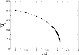
Figure 4: $\overline{M_{s}}$ as functions of the considered values of $J^{\prime}/J$. The dashed lines are added to guide the eye.

III.2 The determination of $\overline{T_{N}}$

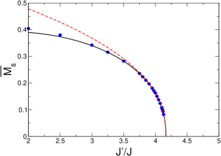
Figure 5: Fits of $\overline{M_{s}}$ to the ansatzes of Eq. (10) (solid line) and a pure power function $a_{1}|j_{c}-j|^{b_{1}}$ (dashed line). The range of $J^{\prime}/J$ and $\chi^{2}/{\text{DOF}}$ for the fit using Eq. (10) (ansatz $a_{1}|j_{c}-j|^{b_{1}}$) are $J^{\prime}/J\geq 3.75$ and 1.2 ($J^{\prime}/J\geq 3.9$ and 1.1), respectively. The leading exponent $b$ of Eq. (10) ($b_{1}$ of $a_{1}|j_{c}-j|^{b_{1}}$) determined from the fit is 0.513(6) (0.42(1)). Applying the ansatz $a_{1}|j_{c}-j|^{b_{1}}$ (Eq. (10)) to fit the data containing those of $J^{\prime}/J\leq 3.5$ ($J^{\prime}/J\leq 2.5$) leads to very poor fitting quality.

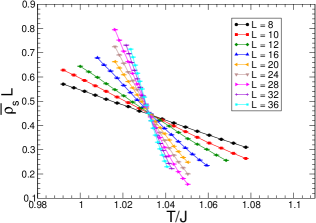
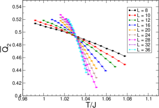
Figure 6: $\overline{\rho_{s}}L$ (top bottom) and $\overline{Q_{2}}$ (bottom panel) as functions of $T/J$ for $J^{\prime}/J=2.0$ and $L$ = 8, 10, 12, 16, 20, 24, 28, 32, 36. $J$ is 1.0 in our calculations. The solid lines are added to guide the eye.

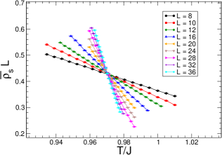
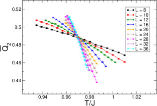
Figure 7: $\overline{\rho_{s}}L$ (top bottom) and $\overline{Q_{2}}$ (bottom panel) as functions of $T/J$ for $J^{\prime}/J=3.0$ and $L$ = 8, 10, 12, 16, 20, 24, 28, 32, 36. $J$ is 1.0 in our calculations. The solid lines are added to guide the eye.

The employed observables for calculating $\overline{T_{N}}$ are $\overline{\rho_{s}}L$, $\overline{Q_{1}}$, as well as $\overline{Q_{2}}$. Notice a constraint standard finite-size scaling ansatz of the form $(1+b_{0}L^{-\omega})(b_{1}+b_{2}tL^{1/\nu}+b_{3}(tL^{1/\nu})^{2}+...$), up to second, third, and (or) fourth order in $tL^{1/\nu}$, is adopted to fit the data. Here $b_{i}$ for $i=0,1,2,...$ are some constants and $t=\frac{T-\overline{T_{N}}}{\overline{T_{N}}}$. For some $J^{\prime}/J$, ansatz up to fifth order in $tL^{1/\nu}$ is used. The data of $\overline{\rho_{s}}L$ and $\overline{Q_{2}}$ for $J^{\prime}/J=2.0$ ($J^{\prime}/J=3.0$) are shown in fig. 6 (fig. 7). In addition, the $\overline{Q_{1}}$ data of $J^{\prime}/J=3.8$ and $J^{\prime}/J=3.95$ are presented in fig. 8. For every $J^{\prime}/J$, ansatzes of various order in $tL^{1/\nu}$ are employed to fit several sets of data (Each set of data has different range of $L$). The cited values of $\overline{T_{N}}$ in this study are estimated by averaging the corresponding results of good fits. Furthermore, the error bar of each quoted $\overline{T_{N}}$ is determined from the uncertainty of every individual $\overline{T_{N}}$ of the associated good fits. For this analysis we consider a fit with $\chi^{2}/{\text{DOF}}\lessapprox 2.0$ a good fit. In some cases, more restricted conditions on $\chi^{2}/{\text{DOF}}$ and the obtained results are imposed for consistency. The determined $\overline{T_{N}}$ from the observables $\overline{\rho_{s}}L$, $\overline{Q_{1}}$, and $\overline{Q_{2}}$ are shown in fig. 9 Tan16 . In addition to $\overline{T_{N}}$, other interesting physical quantities to study are the critical exponents $\nu$ and $\omega$ appearing in the relevant finite-size scaling ansatzes. Notice the dimensionality as well as some critical exponents are present in the conventional finite-size scaling ansatz involving $\rho_{s}$. Based on the analysis of $\overline{M_{s}}$ in previous section, while it is plausible to employ the conventional finite-size scaling ansatz of clean models for the considered finite-temperature phase transitions, one cannot rule out the possibility that when $J^{\prime}/J$ is close enough to the critcal point, the effective dimensions of the system as well as the values of the exponents in the scaling ansatz receive corrections due to the employed disorder. On the other hand, because of their definition, Binder ratios, like $\overline{Q_{1}}$ and $\overline{Q_{2}}$ calculated here, do not encounter such kind of subtlety. Indeed, the values of $\nu$ obtained from the fits related to $\overline{\rho_{s}}L$ are systematic smaller than the corresponding results associated with $\overline{Q_{1}}$ and $\overline{Q_{2}}$. Such a trend is becoming more clear as one approaches the quantum critical point $(J^{\prime}/J)_{c}$. Hence here we only summarize the results of $\nu$ obtained from fitting the data of $\overline{Q_{1}}$ and $\overline{Q_{2}}$ to their expected ansatzes Tan16.1 . The individual average $\nu$ of $J^{\prime}/J$ with $J^{\prime}/J<4.0$, obtained from the related good fits of $\overline{Q_{1}}$ ($\overline{Q_{2}}$), ranging from $0.69$ to $0.72$ (0.69 to 0.73). On the other hand, the values of $\nu$ calculated for $4.0\leq J^{\prime}/J\leq 4.12$ ($J^{\prime}/J=4.13$) lie(s) between 0.63 and 0.69 (0.60 and 0.62). We attribute this result to the fact that data of large box size are limited for $J^{\prime}/J\geq 4.0$. Such scenario is observed for clean dimerized models as well Wen08 ; Jia12 . Finally, the determination of $\omega$ with reasonable precision is hindered by the strong correlation between $\omega$ and its related prefactor $b_{0}$ in the fitting formulas.

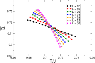
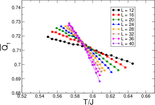
Figure 8: $\overline{Q_{1}}$ as functions of $T/J$ for $J^{\prime}/J=3.8$ (top panel) and $J^{\prime}/J=3.95$ (bottom panel). The box sizes $L$ for these two values of $J^{\prime}/J$ are $L$ = 8, 10, 12, 16, 20, 24, 28, 32, 36 (and 40 for $J^{\prime}/J=3.95$). $J$ is 1.0 in our calculations. The solid lines are added to guide the eye.

After obtaining the numerical values of $\overline{T_{N}}$, we turn to the study of whether a logarithmic correction, like the one associated with $\overline{M_{s}}$, exists for $\overline{T_{N}}$ when $\overline{T_{N}}$ is treated as a function of $J^{\prime}/J$. Similar to our earlier analysis for $\overline{M_{s}}$, we use two ansatzes, namely

$$a_{2}|j_{c}-j|^{b_{2}}$$

$$a_{3}|j_{c}-j|^{b_{3}}|\ln(|(j_{c}-j)/j_{c}|)|^{3/11}$$ (11)

to fit the data of $\overline{T_{N}}/\overline{J}$ determined from all the calculated observables $\overline{Q_{1}}$, $\overline{Q_{2}}$ and $\overline{\rho}_{s}L$. Notice the exponent $b_{3}$ of the second ansatz of Eq. (11) is predicted to take its mean-field value 0.5. Furthermore, we investigate the physical quantity $\overline{T_{N}}/\overline{J}$ instead of $\overline{T_{N}}$ is motivated by the analysis done in Yan15 . The consideration of $\overline{T_{N}}/\overline{J}$ is also natural since it is a dimensionless quantity. Interestingly, for all three data sets, we arrive at good fits ($\chi^{2}/{\text{DOF}}\leq 1.0$) using the second ansatz of Eq. (11) when data points of $\overline{T_{N}}/\overline{J}$ with $J^{\prime}/J\geq 3.75$ are included in the fits. On the other hand, the results obtained from applying the first ansatz to fit the data have much worse fitting quality. As fewer data are included in the fits, while the results related to the second ansatz remain good, the $\chi^{2}/{\text{DOF}}$ associated with the fits employing the first ansatz continue to be very large (except those of the fits using data sets close to $(J^{\prime}/J)_{c}$). Notice ocassionally fits with the first ansatz lead to good results, but not in a systematic manner. The exponent $b_{3}$ and the critical point $(J^{\prime}/J)_{c}$ obtained from all the good fits are given by 0.49(1) and 4.166(2) on the average, respectively. The calculated value of $b_{3}$, namely $b_{3}=0.49(1)$ is in reasonably good agreement with the expected mean-field result 0.5. A fit of this analysis including the logarithmic correction is shown in fig. 10. According to what have been reached so far, we conclude that our data are fully compatible with the scenario that the upper critical dimension, associated with the relevant quantum phase transition of our model, is the same as that of the corresponding clean model. In particular, the related critical exponents are in agreement with the theoretical predictions of clean systems.

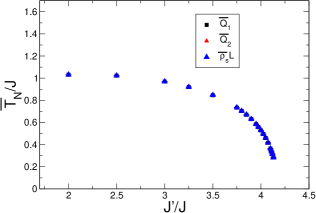
Figure 9: $\overline{T_{N}}$, obtained from $\overline{Q_{1}}$, $\overline{Q_{2}}$, and $\overline{\rho_{s}}L$, as functions of $J^{\prime}/J$.

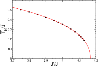
Figure 10: Fit of $\overline{T_{N}}/\overline{J}$ data (obtained from $\overline{Q_{1}}$) with $J^{\prime}/J\geq 4.0$ to their theoretical expression with a logarithmic correction $a_{3}|j_{c}-j|^{b_{3}}|\ln(|(j_{c}-j)/j_{c}|)|^{3/11}$. The $b_{3}$ obtained from the fit is given by 0.494(8).

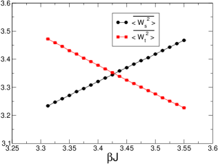
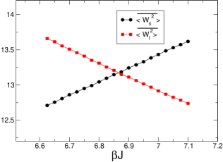
Figure 11: The spatial and temporal winding numbers squared, as functions of $\beta J$ at $J^{\prime}/J=3.0$, for $L=8$ (top panel) and $L=16$ (bottom panel). $J$ is 1.0 in our simulations.

III.3 The determination of $\overline{c}$

The values of spinwave velocity $\overline{c}$ are estimated using the idea of winding numbers squared as suggested in Refs. Jia11 ; Sen15 . Specifically, for a given $J^{\prime}/J$ and a box size $L$, one varies the inverse temperature $\beta$ so that the spatial and temporal winding numbers squared ($\overline{\langle W_{s}^{2}\rangle}=\frac{1}{3}(\overline{\langle W_{1}^{2}\rangle+\langle W_{2}^{2}\rangle+\langle W_{3}^{2}\rangle}$) and $\overline{\langle W_{t}^{2}\rangle}$) take the same values. Assuming one reaches the condition $\overline{\langle W_{s}^{2}\rangle}=\overline{\langle W_{t}^{2}\rangle}$ at an inverse temperature $\beta^{\star}$, then the spinwave velocity $\overline{c}(J^{\prime}/J,L)$ corresponding to this set of parameters $J^{\prime}/J$ and $L$ is given by $\overline{c}(J^{\prime}/J,L)=L/\beta^{\star}$. Notice with our implementaion of configurational disorder, the three spatial winding numbers squared take the same values after one carries out the disorder average. For the $J^{\prime}/J$ of smaller magnitude, the convergence of $\overline{c}$ to their infinite volume values are checked using the data of $L=8$ and $L=16$. In addition, the bulk $\overline{c}$ for large magnitude $J^{\prime}/J$ are obtained from the data of $L=12$ and $L=24$. With the statistics reached here, we find that for all the considered $J^{\prime}/J$ the corresponding bulk spinwave velocities $\overline{c}$ can be correctly given by the results at $L=16$ or $L=24$. The convergence of the spinwave wave velocities to their bulk values for $J^{\prime}/J=3.0$ and $J^{\prime}/J=3.9$ are demonstrated in figs. 11 and 12, respectively, and the bulk $\overline{c}$ we obtain are presented in fig. 13. We would like to point out that for $J^{\prime}/J\geq 4.0$, our estimated central values of $\overline{c}$ for $L=12$ and $L=24$ differ by only less than 0.34 percent and are within their corresponding error bars. Therefore the results of $\overline{c}$ shown in fig. 13 should be very reliable.

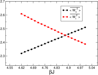
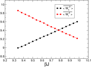
Figure 12: The spatial and temporal winding numbers squared, as functions of $\beta J$ at $J^{\prime}/J=3.9$, for $L=12$ (top panel) and $L=24$ (bottom panel). $J$ is 1.0 in our simulations.

III.4 The scaling relations $\overline{T_{N}}/\overline{c}^{3/2}=A\overline{M_{s}}$ and $\overline{T_{N}}/\overline{J}=A_{1}\overline{M_{s}}$

Having obtained $\overline{M_{s}}$, $\overline{T_{N}}$, and $\overline{c}$, we move to examine whether the scaling relations $\overline{T_{N}}/\overline{c}^{3/2}=A\overline{M_{s}}$ and $\overline{T_{N}}/\overline{J}=A_{1}\overline{M_{s}}$, which are confirmed for clean system(s), remain true for the model with the introduced configurational disorder studied here. Actually, the validity of these relations for our model is expected, since our data of $\overline{T_{N}}/\overline{J}$ and $\overline{M_{s}}$ are fullly compatible with the theoretical predictions for clean systems, and neither $\overline{c}$ nor $\overline{J}$ receives any logarithmic corrections. Indeed, the obtained results of $\overline{T_{N}}/\overline{c}^{3/2}$, when being treated as a function of $\overline{M_{s}}$, can be fitted to the ansatz of $A\overline{M_{s}}$ using the data with the corresponding $\overline{M_{s}}$ having small magnitude. Furthermore, the prefactor $A$ determined from the fits has an average $A_{\text{avg}}\sim 0.858(4)$. Two outcomes of the fits are demonstrated in fig. 14. Notice both the uncertainties of $\overline{T_{N}}/\overline{c}$ and $\overline{M_{s}}$ are taken into account in the fits. Similarly, close to the quantum phase transition, our data of $\overline{T_{N}}/\overline{J}$ and $\overline{M_{s}}$ do satisfy a linear relation as well, see fig. 15.

One may wonder whether the data of $\overline{T_{N}}/\overline{c}^{3/2}$ can be fitted to the ansatz of the form $A\overline{M_{s}}+B$ with $B$ being consistent with zero. We have applied such analyses to the data obtained close to $(J^{\prime}/J)_{c}$. In particular, we arrive at the result that the constants $B$ determined from the fits satisfy $|B|\lesssim 0.005$ and the magnitude of corresponding uncertainties are comparable with $|B|$. We consider these outcomes as a strong indication that our data of $\overline{T_{N}}/\overline{c}^{3/2}$, as a function of $\overline{M_{s}}$, can be described well by a linear function of $\overline{M_{s}}$ passing through the origin.

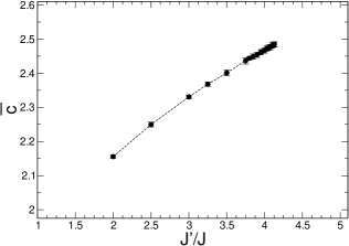
Figure 13: The estimated values of $\overline{c}$ for all the considered $J^{\prime}/J$.

IV Discussions and Conclusions

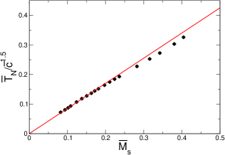
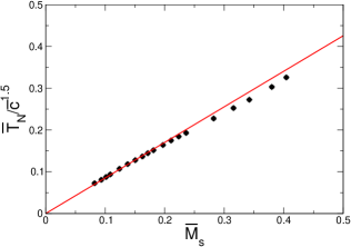
Figure 14: Fits of $\overline{T_{N}}/\overline{c}^{3/2}$ as linear functions of $\overline{M_{s}}$ passing through the origin. The $\overline{T_{N}}$ of the top and bottom panels are obtained from $\overline{Q_{1}}$ and $\overline{Q_{2}}$, respectively.

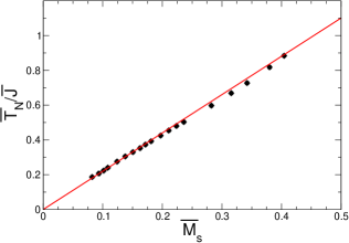
Figure 15: Fit of $\overline{T_{N}}/\overline{J}$ as a linear function of $\overline{M_{s}}$ passing through the origin. The used values of $\overline{T_{N}}$ are obtained from $\overline{Q_{1}}$. The average of the slopes for all the good fits including those resulting from $\overline{Q_{2}}$ and $\overline{\rho_{s}}L$ is given by 2.22(1).

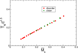
Figure 16: $\overline{T_{N}}/\overline{c}^{3/2}$ as functions of $\overline{M}$ for both the considered disordered model in this investigation and the clean model studied in Ref. Kao13 . The $\overline{T_{N}}$ used in the figure for the disordered model are determined from the observable $\overline{Q_{1}}$.

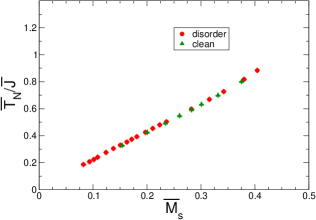
Figure 17: $\overline{T_{N}}/\overline{J}$ as functions of $\overline{M}$ for both the considered disordered model in this investigation and the clean model studied in Ref. Kao13 . The $\overline{T_{N}}$ used in the figure for the disordered model are determined from the observable $\overline{Q_{1}}$.

For clean 3D dimerized quantum Heisenberg models, it is established that the physical quantities $T_{N}/c^{3/2}$ and $T_{N}/\overline{J}$, as functions of $M_{s}$, scale linearly with $M_{s}$. Notice since three spatial dimensions is the upper critical dimensions associated with the related quantum phase transition, one expects there are logarithmic corrections to $T_{N}$ and $M_{s}$ close to the critical point. The linear scaling relations between $T_{N}$ and $M_{s}$ indicate that the exponents associated with the logarithmic corrections to $T_{N}$ and $M_{s}$ take the same values. This result is obtained theoretically in Refs. Ken04 ; Ken12 and is confirmed in Ref. Yan15 .

Motivated by these universal scaling relations between $T_{N}$ and $M_{s}$ for the clean 3D dimerized systems, here we study these relations for a 3D quantum Heisenberg model with configurational disorder. A remarkable result observed in our investigation is that close to the considered critical point, the relations $T_{N}/c^{3/2}=AM_{s}$ and $T_{N}\overline{J}=A_{1}M_{s}$ remain valid for the studied model with the introduced disorder. In addition, both the obtained data of $\overline{T_{N}}$ and $\overline{M_{s}}$ in this study do receive multiplicative logarithmic corrections and are fully compatible with the expected critical behaviour for clean dimerized models. This indicates that the related quantum phase tranistion of the studied system may be described by the same critical theory as that of its clean analogues. In Ref. Yan15 , it is found that for the clean 3D double cubic quantum Heisenberg model the numerical value of the coefficient $A$ in $T_{N}/c^{3/2}=AM_{s}$ is given by $A\sim 1.084$. For the disordered model considered here, the corresponding coefficient is given by $A\sim 0.86$, which is different from $A\sim 1.084$ associated with the double cubic model studied in Ref. Yan15 . Consequently, this coefficient $A$ is likely not universal and depends on the microscopic details of the investigated systems. Interestingly, using the data determined here and that of a clean system calculated in Ref. Kao13 , smooth universal curves associated with the studied scaling relations do show up (See figs. 16 and 17). This implies that while not being generally true, universal coefficients may still exist within models sharing some similar characters. It will be interesting to investigate, in a more quantitative manner, that under what conditions will the coefficients $A$ and $A_{1}$ of different models take the same numerical values. Finally, although based on our investigation we conclude that the coefficient $A$ is likely not universal, we find the quantity $A/(J^{\prime}/J)_{c}^{3/2}$ determined in this investigation matching very well with the corresponding result in Yan15 . Specifically, using the data available in Ref. Yan15 and here, we reach $A/(J^{\prime}/J)_{c}^{3/2}\sim 0.1019$ and $A/(J^{\prime}/J)_{c}^{3/2}\sim 0.1011$ for the double cubic model and the disordered model studied here, respectively. Notice the numerical values of $A/(J^{\prime}/J)_{c}^{3/2}$ obtained from two different models are in very good agreement with each other. While our preliminary result of $A/(J^{\prime}/J)_{c}^{3/2}$ of other dimerized model does not seem to support the scenario that the quantity $A/(J^{\prime}/J)_{c}^{3/2}$ takes a universal value, the investigation carried out in this study suggests true universal quantities may still emerge for both the clean and disordered 3D antiferromagnets (Which share some similar properties). To uncover the possible hidden universal relations of 3D antiferromagnets will be an interesting topic to conduct in the future.

V Acknowledgments

We thank A. W. Sandvik for encouragement. This study is partially supported by MOST of Taiwan.

References

- (1) Nigel Goldenfeld, Lectures On Phase Transitions And The Renormalization Group (Frontiers in Physics) (Addison-Wesley, 1992).
- (2) S. Sachdev, Quantum Phase Transitions (Cambridge University Press, Cambridge, 1999).
- (3) Lincoln D. Carr, Understanding Quantum Phase Transitions (Condensed Matter Physics) (CRC Press, 2010).
- (4) Munehisa Matsumoto, Chitoshi Yasuda, Synge Todo, and Hajime Takayama, Phys. Rev. B 65, 014407 (2002).
- (5) L. Wang, K. S. D. Beach, and A. W. Sandvik, Phys. Rev. B 73, 014431 (2006).
- (6) S. Wenzel, L. Bogacz, and W. Janke, Phys. Rev. Lett. 101, 127202 (2008).
- (7) A. F. Albuquerque, M. Troyer, J. Oitmaa, Phys. Rev. B 78, 127202 (2008).
- (8) S. Wenzel and W. Janke, Phys. Rev. B 79, 014410 (2009).
- (9) F.-J. Jiang and U. Gerber, J. Stat. Mech. P09016 (2009).
- (10) F.-J. Jiang, Phys. Rev. B 85 014414 (2012).
- (11) M. Campostrini, M. Hasenbusch, A. Pelissetto, P. Rossi, and E. Vicari, Phys. Rev. B 65, 144520 (2002).
- (12) Andrea Pelissetto and Ettore Vicari, Physics Reports 368 (2002) 549-727.
- (13) L. Fritz, R. L. Doretto, S. Wessel, S. Wenzel, S. Burdin, and M. Vojta, Phys. Rev. B 83, 174416 (2011).
- (14) S. Chakravarty, B. I. Halperin, and D. R. Nelson, Phys. Rev. Lett. 60, 1057 (1988).
- (15) J. D. Reger and A. P. Young, Phys. Rev. B 37, R5978 (1988).
- (16) S. Chakravarty, B. I. Halperin, and D. R. Nelson, Phys. Rev. B 39, 2344 (1989).
- (17) H. Neuberger and T. Ziman, Phys. Rev. B 39, 2608 (1989).
- (18) P. Hasenfratz and H. Leutwyler, Nucl. Phys. B343, 241 (1990).
- (19) P. Hasenfratz and F. Niedermayer, Phys. Lett. B268, 231 (1991).
- (20) P. Hasenfratz and F. Niedermayer, Z. Phys. B 92, 91 (1993).
- (21) A. V. Chubukov, S. Sachdev, and J. Ye, Phys. Rev. B 49, 11919 (1994).
- (22) U.-J. Wiese and H.-P. Ying, Z. Phys. B 93, 147 (1994).
- (23) M. Troyer, H. Kantani, and K. Ueda, Phys. Rev. Lett. 76, 3822 (1996).
- (24) B. B. Beard and U.-J. Wiese, Phys. Rev. Lett. 77, 5130 (1996).
- (25) A. W. Sandvik, Phys. Rev. B (1997).
- (26) F.-J. Jiang, F. Kampfer, M. Nyfeler, and U.-J. Wiese, Phys. Rev. B 78, 214406 (2008).
- (27) F.-J. Jiang, F. Kämpfer, and M. Nyfeler, Phys. Rev. B 80, 033104 (2009).
- (28) F.-J. Jiang and U.-J.Wiese, Phys. Rev. B 83, 155120 (2011).
- (29) N. Cavadini, G. Heigold, W. Henggeler, A. Furrer, H.-U. Güdel, K. Krämer, and H. Mutka, Phys. Rev. B 63, 172414 (2001).
- (30) Ch. Rüegg, N.Cavadini, A. Furrer, H.-U. Güdel, K. Krämer, H. Mutka, A. Wildes, K. Habicht, and P. Vorderwisch, Nature (London) 423, 62, (2003).
- (31) Ch. Rüegg et al., Phys. Rev. Lett. 100, 205701 (2008).
- (32) Y. Kulik, and O. P. Sushkov, Phys. Rev. B 84, 134418 (2011).
- (33) J. Oitmaa, Y. Kulik, and O. P. Sushkov, Phys. Rev. B 85, 144431 (2012).
- (34) S. Jin and A. W. Sandvik, Phys. Rev. B 85, 020409(R) (2012).
- (35) M.-T. Kao and F.-J. Jiang, Eur. Phy. J. B, (2013) 86: 419.
- (36) P. Merchant, B. Normand, K. W. Krämer, M. Boehm, D. F. McMorrow, and Ch. Rüegger, Nature physics 10, 373-379 (2014).
- (37) Deng-Ruei Tan and Fu-Jiun Jiang, Eur. Phys. J. B, (2015) 88 : 289.
- (38) Harley Scammell and Oleg Sushkov, ArXiv:1605.05460.
- (39) R. Kenna, Nucl. Phys. B 691, 292 (2004).
- (40) R. Kenna, Vol. 3, Chap. 1, in Order, Disorder and Criticality, edited by Y. Holovatch, World Scientific, Singapore, 2012.
- (41) Yan Qi Qin, Bruce Normand, Anders W. Sandvik, and Zi Yang Meng, Phys. Rev. B 92, 214401 (2015).
- (42) Harley Scammell and Oleg Sushkov, Phys. Rev. B 92, 220401 (2015).
- (43) O. P. Vajk, P. K. Mang, M. Greven, P. M. Gehring, and J. W. Lynn, Science 295, 1691 (2002).
- (44) T. Vojta, J. Low Temp. Phys. 161, 299 (2010).
- (45) Dao-Xin Yao, Jonas Gustafsson, E. W. Carlson, and Anders W. Sandvik, Physical Review B, 82, 172409 (2010).
- (46) A. W. Sandvik, Phys. Rev. B 66, R14157 (1999).
- (47) A. W. Sandvik, Phys. Rev. B 66, 024418 (2002).
- (48) J. Cardy, Scaling and Renormalization in Statistical Physics (Cambridge University Press, Cambridge, 1996).
- (49) In an early version of this manuscript, we claimed that for the close to , the corresponding values of determined from deviate slightly from those associated with the Binder ratios. With higher order ansatzes, careful investigation of deciding data range for the fits, and more statistics, now the discrepancies disappear for most of the considered . Consequently, some numerical analysis are redone and the corresponding results are updated. Conclusions remain the same.
- (50) While it is likely that the determination of by considering the observable is affected by the presence of bond disorder, the quantitative agreement among the obtained from , , and indicates that the calculated results of are reliable.
- (51) F.-J. Jiang, Phys. Rev. B 83, 024419 (2011).
- (52) A. Sen, H. Suwa, and A. W. Sandvik, Phys. Rev. B 92, 195145 (2015).