Volatiles beneath mid-ocean ridges: deep melting, channelised transport, focusing, and metasomatism

Abstract

Deep-Earth volatile cycles couple the mantle with near-surface reservoirs. Volatiles are emitted by volcanism and, in particular, from mid-ocean ridges, which are the most prolific source of basaltic volcanism. Estimates of volatile extraction from the asthenosphere beneath ridges typically rely on measurements of undegassed lavas combined with simple petrogenetic models of the mean degree of melting. Estimated volatile fluxes have large uncertainties; this is partly due to a poor understanding of how volatiles are transported by magma in the asthenosphere. Here, we assess the fate of mantle volatiles through numerical simulations of melting and melt transport at mid-ocean ridges. Our simulations are based on two-phase, magma/mantle dynamics theory coupled to an idealised thermodynamic model of mantle melting in the presence of water and carbon dioxide. We combine simulation results with catalogued observations of all ridge segments to estimate a range of likely volatile output from the global mid-ocean ridge system. We thus predict global MOR crust production of 66–73 Gt/yr (22–24 km³/yr) and global volatile output of 52–110 Mt/yr, corresponding to mantle volatile contents of 100–200 ppm. We find that volatile extraction is limited: up to half of deep, volatile-rich melt is not focused to the axis but is rather deposited along the LAB. As these distal melts crystallise and fractionate, they metasomatise the base of the lithosphere, creating rheological heterogeneity that could contribute to the seismic signature of the LAB.

1 Introduction

1.1 Deep volatile cycles

Deep-Earth volatile cycles are a result of fluxes between near-surface, shallow-mantle and deep-mantle reservoirs. These fluxes are associated with transport processes in the solid Earth that may be modified by the volatiles themselves (e.g., Hirth and Kohlstedt, 1996; Dasgupta and Hirschmann, 2010). Volatile cycles impact aspects of planetary dynamics including mantle convection and partial melting. Partial melting is the key process by which volatiles are released from the mantle to near-surface reservoirs; it influences deep and shallow phenomena including the formation of the oceanic (Hirth and Kohlstedt, 1996; Asimow et al., 2004) and continental crust (Müntener et al., 2001; Ulmer, 2001), the long-term tectonic regime of a planet (Mian and Tozer, 1990; Regenauer-Lieb, 2001) and, potentially, variations of the surface climate (Huybers and Langmuir, 2009; Crowley et al., 2015; Burley and Katz, 2015; Tolstoy, 2015; Huybers and Langmuir, 2017). The thermodynamic effect of mantle volatiles on partial melting and, in particular, that of water and carbon dioxide, is now well documented (e.g., Hirschmann et al., 1999; Asimow and Langmuir, 2003; Dasgupta et al., 2013). A key problem, however, remains almost unexplored: the dynamics of melt transport in the presence of volatiles. A theoretical framework to investigate these dynamics has recently been developed by Keller and Katz (2016).

Volatile-enriched partial melting and melt transport is relevant to all environments in which partial melting occurs; perhaps most of all to subduction zones, where melt production is primarily driven by the input of volatiles. In this manuscript, however, we focus on divergent plate margins, which are a simpler geodynamic context. The mid-ocean ridge (MOR) system is the primary avenue for volatile extraction from the mantle (Resing et al., 2004; Dasgupta and Hirschmann, 2010; Kelemen and Manning, 2015). A simple estimate of the volatile output from ridges is the product of the formation rate of oceanic crust ($\sim 24$ km³/yr or 72 Gt/yr, Crisp (1984)) and the mean volatile concentration in undegassed primary mid-ocean-ridge basalt (MORB) (e.g., Michael and Graham, 2015; Rosenthal et al., 2015). Resing et al. (2004) constrain the MOR CO₂ emission rate to a range of 22–88 Mt CO₂/yr, Dasgupta and Hirschmann (2010) produce estimates of 46–324, Cartigny et al. (2008) of 44–220, and Kelemen and Manning (2015) of 29–154 Mt CO₂/yr. Some of these include contributions from oceanic intraplate volcanism.

Such estimates are the basis for currently accepted volatile output from ridges, but bypass important considerations. For example, relating fluxes to the concentration of volatiles in the sub-ridge mantle requires constraints on the locus of partial melting in the mantle as well as on the efficiency of volatile transport with ascending melts. Also, simple budget calculations cannot constrain the fraction of volatile-rich melts that are emplaced into the oceanic lithosphere rather than focused to the ridge axis. Any such emplaced melts may influence the properties of the oceanic lithosphere and contribute to volatile release during subduction. Moreover, mean flux estimates do not allow exploration of dynamic controls such as viscosity and permeability (Braun et al., 2000; Kono et al., 2014), channelised flow (Kelemen et al., 1995), and spatial variations in mantle potential temperature and composition (Dalton et al., 2014).

1.2 Volatiles in mid-ocean ridge magmatism

Small concentrations of volatiles greatly expand the volume of mantle that produces partial melt beneath ridges by causing melting to initiate at greater depths. For typical sub-ridge potential temperatures, volatile-free melting may occur above 60–75 km, but as little as 100 ppm H₂O depresses the onset of melting to 100–120 km depth (Hirth and Kohlstedt, 1996; Hirschmann et al., 1999). Comparable amounts of CO₂ lead to an onset of melting between 150 and 300 km depth, depending on the redox state of the mantle (Dasgupta and Hirschmann, 2010). Moreover, due to the widening of the upwelling region with depth (Lachenbruch, 1976; Spiegelman and McKenzie, 1987), deepening the melting regime produces small fractions of melt at considerable lateral distance away from the axis. These distal, low-degree melts are rich in incompatible trace elements as well as in volatiles. The proportion of distal melts that are focused to the ridge axis rather than frozen into growing oceanic lithosphere or erupted at off-axis seamounts is uncertain (Galer and O’Nions, 1986; Plank and Langmuir, 1992). Furthermore, erupted MORB has long been considered a mixture of polybaric melts, the composition of which is sensitive to the shape of the melting regime (O’Hara, 1985; Plank and Langmuir, 1992; Asimow and Langmuir, 2003). Lastly, the consequences of rheological weakening by volatiles are not yet well understood (Hirth and Kohlstedt, 1996; Braun et al., 2000). Resolving the dynamic aspects of MORB petrogenesis therefore requires an improved understanding of the reactive segregation of deep, volatile-rich melts.

Such deep melting produces melt fractions much less than 1% (e.g., Plank and Langmuir, 1992; Hirth and Kohlstedt, 1996; Asimow et al., 2004; Dasgupta and Hirschmann, 2006). Evidence from short-lived radiogenic products of uranium decay (²³⁰Th, ²³¹Pa, and ²²⁶Ra) indicates that very small melt fractions segregate from their deep sources and ascend rapidly to the surface (Spiegelman and Elliott, 1993; McKenzie, 2000; Elliott and Spiegelman, 2003). This may be facilitated by high-permeability melt channels (Aharonov et al., 1995; Spiegelman et al., 2001). Keller and Katz (2016) showed that such channels may form when deep, volatile-rich melt fluxes the primary basaltic melting regime from below. Quantifying the consequences of incipient melting, channelised melt transport, and magmatic focusing on MOR volatile output is the goal of this study.

1.3 Method summary

We use two-dimensional numerical simulations of two-phase, multi-component, reactive flow in the asthenosphere to model magma genesis and transport beneath a MOR. The model is calibrated to reproduce accepted features of melting in an upwelling mantle containing H₂O and CO₂ in low concentrations. Crustal thickness is used as an observational constraint on MOR models (White et al., 2001); we generate predictions for comparison with data by computing the rate at which magma is delivered to the ridge axis. To scale our model results from individual instances to the ensemble of ridge segments that comprise the global MOR system, we use a catalogue of kinematic, chemical, and thermal parameters compiled by Gale et al. (2014) and Dalton et al. (2014). Empirical scaling laws fitted to the output of dynamic simulations are combined with this catalogued data to create estimates of crust production and volatile extraction for the global MOR system.

Section 2 introduces the computational model used to generate simulations and discusses the leading-order features and parametric controls of their output. Section 3 discusses melt focusing, crust production and volatile extraction predicted by simulations; section 4 develops estimates of global MOR volatile output; metasomatism of the oceanic lithosphere is considered in section 5. Section 6 summarises our findings and offers some conclusions.

2 Mid-ocean ridge simulations

2.1 Theory, parameters, and numerical solutions

Simulations are based on numerical solutions to a system of partial differential equations comprising statements of mass, momentum, and energy conservation for two phases (liquid and solid), and four thermochemical components. Solutions are computed on a two-dimensional domain representing half of a symmetrical spreading center. The domain extends to a depth of 200 km and a width of 300 km from the axis. Model derivation and numerical implementation are given in Keller and Katz (2016); the theory is built upon that of McKenzie (1984) and Rudge et al. (2011).

Magma and rock compositions are modelled in a four-component compositional space of DUN $+$ MORB $+$ hMORB $+$ cMORB. These chemical components represent the residue of mantle melting (dunite), the product of volatile-free decompression melting (basalt), and the products of hydrated and carbonated melting at depth (hydrated, carbonated basalt), respectively. The latter two components contain volatiles at fixed concentrations of 5 wt% H₂O in hMORB, and 20 wt% CO₂ in cMORB. Linear kinetic reaction rates are calculated with the R_DMC method (Keller and Katz, 2016, 2015), using a constant rate factor of $\mathcal{R}=3$ kg/m³/yr (corresponding to a reaction time of $\sim$1 kyr). Density is taken as constant and uniform for both phases, except in body-force terms where a density difference between melt and solid of $\Delta\rho=500$ kg/m³ drives segregation. See Appendix A for a summary of the R_DMC model for thermodynamic equilibrium and melt-rock reactions.

The viscosity of mantle rock is reduced by water and melt (Hirth and Kohlstedt, 1996; Mei et al., 2002), and volatile-bearing silicate melt is weakened by both H₂O and CO₂. Permeability depends on grain size and melt fraction according to the Kozeny-Carman relation. For details of constitutive laws see Appendix B.

Plate spreading at a half-rate $u_{0}$ is imposed along the top boundary of the model domain; the bottom and off-axis side boundaries are open to inflow and outflow of the mantle in passive response to plate spreading. Symmetry conditions are applied along the vertical boundary beneath the ridge axis. Melt extraction at the axis occurs through an imposed patch of $4\times 8$ km size where melting and freezing reactions are disallowed. For numerical convenience, a maximum solidus depth of 160 km is imposed to keep the lower boundary of the domain melt-free at all times.

Calculations are initialised with the temperature solution to the plate-cooling half-space problem. Some pre-depletion of the mantle composition is imposed in the melting region. The initial temperature is then limited point-wise by the solidus temperature such that the melt fraction is initially zero. These arrangements minimise the time required for model evolution from the initial condition to an approximately steady state (the “spin-up” time) (Katz, 2008, 2010).

Simulations at reference resolution of 1 km per grid cell have a numerical problem size of 744k degrees of freedom and are computed on 64 cores of the BRUTUS cluster at ETH Zurich, Switzerland. Numerical solutions are obtained using a parallel Newton-Krylov method leveraging the PETSc toolkit (Balay et al., 2011, 2010; Katz et al., 2007).

2.2 Reference model

The reference model simulates an intermediate-spreading ridge with $u_{0}=3$ cm/yr, a mantle potential temperature $T_{m}=1350$ ^∘C, and a mantle bulk composition $\bar{c}^{i}$ (in wt%) of 74.75 DUN, 25 MORB, 0.2 hMORB, and 0.05 cMORB. The concentrations of the latter two correspond to volatile contents of 100 wt ppm each of H₂O and CO₂. A white-noise perturbation field is low-pass filtered to a minimum wavelength of $\sim$5 km and used to add compositional heterogeneity in mantle fertility (MORB content) at a relative amplitude of $\pm$10%. The identical perturbation is used to introduce mantle heterogeneity in all simulations reported here.

Figure 1 shows a snapshot of the reference model after 10 Myr. At this stage, plate spreading and mantle upwelling have swept the full width and depth of the domain and thus dynamics have evolved well past the effects of initial conditions. The general features of the magmatic system are representative of all simulations presented here. A key feature is the coalescing network of magmatic channels focusing melt towards the ridge axis. These channels are most notable across a depth range of 50–80 km below the ridge axis and are characterised by increased melt fraction (panel (a)), magnitude of Darcy flux $|\mathbf{q}|=\phi|\mathbf{v}_{\ell}-\mathbf{v}_{s}|$ (panel (b)), and volatile concentrations (panels (c) & (d)).

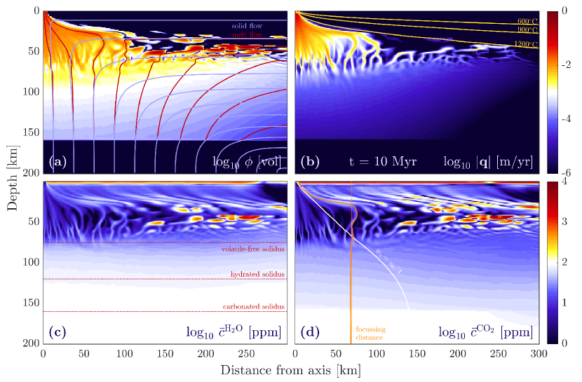
Figure 1: Output from reference simulation at 10 Myr. Panels show (a) melt fraction, with melt (red) and solid (blue) streamlines; (b) Darcy flux magnitude, with 600, 900 and 1200 ^∘C isotherms; (c) bulk water concentration, with calibrated solidus depths for volatile-free, hydrated and carbonated mantle; (d) bulk carbon dioxide concentration, with contour of primary upwelling and melt producing domain (white) and melt streamline delimiting the melt focusing domain (orange), with equilibrium focusing distance $x_{e}$ (dotted) for comparison.

The network is formed of reactive-dissolution channels as described in Keller and Katz (2016). Channelisation is driven by the corrosivity of deep, low-degree, volatile-rich melts. These melts flux the base of the volatile-free melting regime where they create a Reactive Infiltration Instability (Aharonov et al., 1995; Szymczak and Ladd, 2014). Enhanced flux of deep melt leads to dissolution of the MORB component, increased porosity and permeability, and further enhancement of melt flux. Reactive channels thus form approximately parallel to the melt flow direction.

Figure 2 shows a comparison of the Darcy flux in simulations with volatile contents of 0, 50, 100 (ref. case), and 200 ppm. The distributed flow regime in the volatile-free case of panel (a) indicates that the perturbation of the compositional field does not itself cause channelisation. However, with increasing volatile content (panels (b)–(d)) the degree of flow localisation increases. This trend reinforces the argument that the presence of volatile elements in the mantle source causes channelisation. In our calculations, as little as 50 ppm each of H₂O and CO₂ is sufficient to initiate channelling. This value is at the low end of estimates for the MORB-source mantle.

Figure 2: Darcy flux magnitude $|\mathbf{q}|$ at $t=10$ Myr for simulations with (a) no volatiles, (b) 50 ppm, (c) 100 ppm (reference), and (d) 200 ppm each H₂O and CO₂ in the mantle source. Streamlines for melt (red) and solid (blue) flow, outline of primary upwelling domain (black), and melt focusing domain (orange), with $x_{e}$ (dotted) for comparison.

2.3 Volatile extraction by melt focusing

Volatile-rich melt is produced over a broad region beneath the volatile-free melting regime. Extraction of these deep melts depends on the efficiency of melt focusing towards the ridge axis. Interpretation of observed volatile contents of MORBs therefore requires a model, whether implicit or explicit, of melt extraction from the melting regime. The canonical model of MORB petrogenesis analyses melting and melt focusing in terms of the residual mantle column (RMC) — the lateral solid outflow from the melting regime, after steady-state melt extraction (e.g., Klein and Langmuir, 1987; McKenzie and Bickle, 1988; Plank and Langmuir, 1992). Figure 3 juxtaposes this model (left-hand side) against a conceptual model derived from simulations presented here (right-hand side).

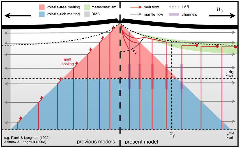
Figure 3: Summary of melt focusing beneath a MOR. Shaded areas show volatile-bearing (blue) and volatile-free (red) domains decompression melting; reactive channelling (purple); area of crystallisation and metasomatism (green). Dotted lines mark depths of first melting for volatile-bearing, $z_{\mathrm{sol}}^{\mathrm{vol}}$, volatile-free mantle, $z_{\mathrm{sol}}^{\mathrm{dry}}$; lateral melt focusing distance $x_{f}$; active focusing radius $r_{f}$. Melt (red) and solid (grey) flow paths are strongly simplified. Left hand side presents simplified standard model, compared to model presented in this study on the right hand side. The key difference is the fate of deep, volatile-rich melt.

Plank and Langmuir (1992) and Asimow and Langmuir (2003) calculate volume and composition of extracted melt using the RMC (Fig. 3, left). All melt produced within a chosen focusing distance from the ridge is assumed to arrive at the axis, a concept referred to by the authors as “melt pooling.” Volume and composition of extracted melt are calculated as a weighted sum of melts produced at various pressures and degrees of melting (Langmuir et al., 1992). Although most of the calculations in Plank and Langmuir (1992) assume perfect focusing of distal melts, they recognised that “it is especially difficult to envision efficient extraction and focusing over hundreds of kilometers;” they discuss these difficulties in some detail. Asimow and Langmuir (2003) do not consider the limits of focusing; their calculations pool melts from the entire melting regime by integrating over the full depth of the RMC.

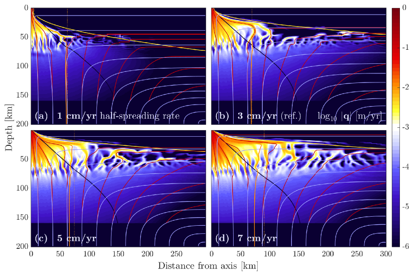
Figure S1: Darcy flux magnitude $|\mathbf{q}|$ at $t=10$ Myr for simulations with half-spreading rates of (a) 1 cm/yr, (b) 3 cm/yr (reference), (c) 5 cm/yr, and (d) 7 cm/yr. Streamlines for melt (red) and solid (blue) flow, outline of primary upwelling domain (black), and melt focusing domain (orange), with $x_{e}$ (dotted) for comparison. Faster spreading rates lead to shallower temperature structure and higher melt production reflected in increased Darcy flux. The focusing distance grows with spreading rate. Note that the primary upwelling contours consistently intersect with the proxies for melt focusing distance around the volatile-free solidus depth at $\sim$70 km.

In the present calculations, melt focusing is not an assumption but rather a consequence of model dynamics. Careful analysis of results suggests that focusing arises by two mechanisms, represented schematically on the right-hand side of Fig 3 (c.f. Suppl. Figs S1–S3). Melt ascends by vertical porous flow driven by melt buoyancy. As it approaches the thermal boundary layer along the LAB, crystallisation and increasing rock viscosity prohibit further vertical ascent. Instead, melt is diverted towards the axis, continuing as gravity-driven flow in a decompaction channel along the LAB (Sparks and Parmentier, 1991; Montési et al., 2011). We refer to this first mechanism as passive focusing. The passive focusing distance $x_{f}$ arises from balancing rates of melt supply from beneath and loss to freezing into the base of the spreading plate; it is modulated by the slope of the LAB (e.g., Katz, 2008; Hebert and Montési, 2010).

Under the second mechanism, plate spreading induces a dynamic pressure gradient that focuses melt transport toward the axis (Spiegelman and McKenzie, 1987); we refer to this as active focusing. It extends radially from the ridge to a radius $r_{f}$. Inside this radius, melt streamlines curve away from the thermal boundary on the ridge flanks, pointing down the dynamic pressure gradient towards the axis. The focusing radius scales with the compaction length,

$$\delta_{c}=\sqrt{\zeta K/\mu}\>,$$ (1)

where $K$ is the permeability, and $\eta$ and $\zeta$ the shear and compaction viscosities, assuming $\zeta\gg\eta$. In two-phase dynamics, pressure perturbations decay away from an applied forcing over a length scale of approximately the compaction length (McKenzie, 1984). Depending on assumptions about permeability, compaction viscosity and melt viscosity, and for melt fractions of 0.1–1 wt%, $\delta_{c}$ in the asthenosphere may be of order 1–100 km (see Appendix B).

Conductive heat flux to the surface causes cooling along the flanks of the melting regime. Some melt pathways will traverse these regions, where cooler temperatures cause deep fractional crystallisation. As a consequence, volatiles (and other incompatibles) become more enriched in these melts. Hence the volatile content of focused melts depends to some degree on their focusing pathways, which in turn are controlled by the two focusing mechanisms above. Previous models did not include these effects or their consequences for volatile extraction.

For parameter ranges considered here, the active focusing radius is typically smaller than the passive focusing distance. Thus $x_{f}$ marks the outer boundary of the melt focusing domain. The melt streamline in Fig. 1(d) approximately marks the path of the most distal melt still focused to the axis. We use the distance at which it intersects the base of the melting regime as a proxy for $x_{f}$. Katz (2008) proposed an independent measure of $x_{f}$ based on integrated mass fluxes; it is termed the equilibrium focusing distance $x_{e}$ (orange dotted, Fig. 1(d)). Both measures typically produce consistent estimates. $x_{f}$ correlates well with the lateral distance where the $u_{0}/3$ isopleth of solid upwelling rate intersects the volatile-free solidus depth (white line in Fig. 1(d)). At reference parameters, we find $x_{f}\approx 65$ km.

Model results suggest that the primary effects of volatiles — deeper onset of melting, a broader melting regime and reactive channelisation — do not have any significant effect on melt focusing. Thus, only volatile-rich melt produced in the central parts of the deep melting regime reaches the MOR axis. This result differs sharply from assumptions of Asimow and Langmuir (2003) and similar models. Furthermore, although volatiles cause channelisation of melt flow, this does not affect melt focusing: channels emerge in alignment with the prior direction of melt transport. The main effect of channelised melt transport is instead to increase the spatial and temporal variability of melt flux and composition.

Melt focusing that is independent of deep, volatile-rich melting limits the efficiency of volatile extraction relative to previous estimates (e.g., Asimow and Langmuir, 2003). Basalt extracted at the axis is therefore dominated by low-pressure, high-degree melt. Most of the low-degree melt produced in the distal wings of the volatile-rich melting regime, conversely, migrates towards the LAB. There it is collected into lenticular bodies with melt fraction of 5–50 wt% at 20–60 km depth (Fig. 1(a)). These liquids metasomatise the base of the lithosphere. As they crystallise and fractionate, their volatile content increases while their freezing point decreases. We discuss these effects in section 5, below.

3 Quantifying volatile extraction

3.1 Melt production and focusing

To quantify production and focusing of melt in MOR simulation results we calculate the following rates of mass transfer per unit length of MOR axis: $q_{\mathrm{base}}^{i}$, the flow rate of component mass into the base of the melting regime ($z_{\mathrm{sol}}=160$ km); $q_{\mathrm{melt}}^{i}$, the rate of component mass transfer by melting over the full melting regime; $q_{\mathrm{focus}}^{i}$, the rate of component mass delivery to the ridge axis. Their calculation is discussed in Appendix C.

The ratios $R_{\mathrm{melt}}^{i}$ and $R_{\mathrm{focus}}^{i}$ are then introduced to quantify the mean degree of melting beneath the ridge and the efficiency of melt focusing to the axis. The melt production ratio $R_{\mathrm{melt}}^{i}$ is the time-averaged melt production rate divided by the time-averaged mantle inflow rate. The melt focusing ratio $R_{\mathrm{focus}}^{i}$ is the time-averaged melt focusing rate divided by the time-averaged melt production rate. These ratios are calculated for each component and for the bulk mantle as

$$R_{\mathrm{melt}}^{i} =\dfrac{\langle q_{\mathrm{melt}}^{i}\rangle}{\langle q_{\mathrm{base}}^{i}\rangle}\>,$$ (2a)

$$R_{\mathrm{focus}}^{i} =\dfrac{\langle q_{\mathrm{focus}}^{i}\rangle}{\langle q_{\mathrm{melt}}^{i}\rangle}\>,$$ (2b)

where $\langle\cdot\rangle$ denotes a time average.

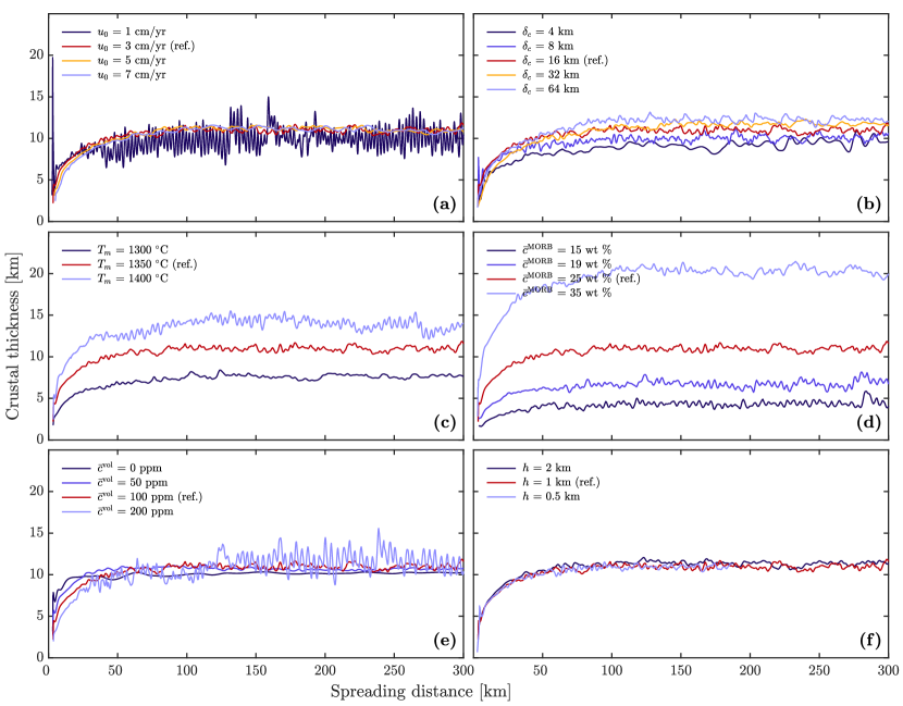
Figure S4: Time series of crustal thickness for all parameter choices. Results plotted against spreading distance. Time averages extracted over interval from 180–300 km. The resolution tests in h show that crust production in the reference case is well resolved at reference conditions.

Time-averaging is used to analyse the mean, long-term behaviour of the ridge apart from internal fluctuations. The time interval over which averages are taken corresponds to plate spreading distances between $x_{0}=180$ km and the full width of the model domain $x_{1}=W=300$ km. By that interval, plate spreading and solid upwelling have swept once through the melt regime, and visual inspection suggests that transients associated with model spin-up have disappeared (see Suppl. Figs S4–S6). Below, we discuss model output in terms of time-averaged rates $\langle q\rangle$ (and derived quantities) and their standard deviations $\sigma$ across this post-spin- up time interval.

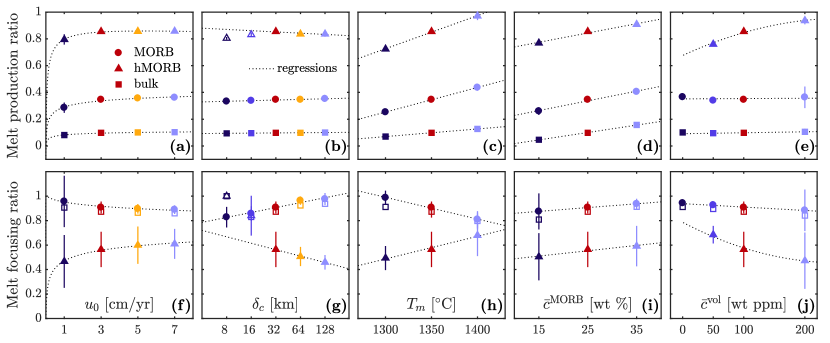
Figure 4: Magmatic ratios from (2) as a function of parameter values. Time-averaged melt production ratios for MORB (circles), hMORB (triangles), and bulk mantle (squares). Results are plotted as a function of: (a) half-spreading rate; (b) compaction length; (c) potential temperature; (d) fertility; (e) volatile content. Time-averaged melt focusing ratios for MORB (circles), and hMORB (triangles), and bulk mantle (squares). Bars indicate $\pm 2\sigma$. Dotted lines are regressions of the simulation output. Open symbols not included in regressions.

Figure 4 shows time-averaged melt production and focusing ratios plotted against model parameters including spreading rate, compaction length, mantle temperature, fertility, and volatile content. Parameter variations are applied one parameter at a time with other parameters held at reference values. Variations span a range of 1–7 cm/yr in half-spreading rate, 8–128 km in compaction length (see Appendix B), 1300–1400 ^∘C in mantle temperature, 15–35 wt% in mantle fertility (MORB content), and 0–200 ppm in volatile content (H₂O and CO₂ added as hMORB and cMORB).

The bulk melt production ratio is $\sim$10%. This is comparable to the mean degree of melting discussed by Asimow and Langmuir (2003). $R_{\mathrm{melt}}^{i}$ correlates positively with mantle temperature and fertility but is largely independent of spreading rate (at least for slow to fast spreading ridges), compaction length and volatile content. We do not observe a lowering of $R_{\mathrm{melt}}^{i}$ with the addition of volatiles, as described for the mean degree of melting by Asimow and Langmuir (2003). This difference comes from normalising $R_{\mathrm{melt}}^{i}$ by mantle inflow at a fixed depth (160 km) rather than the volatile-dependent depth of first melting used by Asimow and Langmuir (2003).

The melt production ratios for the hMORB and MORB component illustrate the difference between volatile-rich and volatile-free melt production. While the former shows degrees of melting of 0.85–0.95, the latter only reaches 0.25–0.4. The dissolution of the incompatible, water-rich component from the partially molten asthenosphere is therefore nearly complete in our models. Results for the carbonated component are similar to those for hMORB, and are therefore not shown in Fig. 4. The melts extracted at the ridge axis show no fractionation of water and carbon from their 1:1 source ratio. This is simply due to the high mean degree of melting that dominates the composition of extracted melts.

Plank and Langmuir (1992) considered focusing of distal, volatile-rich melts to be physically implausible. Here, we assess the efficiency of melt focusing and volatile extraction arising from dynamic simulations. Fig. 4(f)–(j) shows melt focusing ratios for the MORB and hMORB components. 80–100% of MORB melt is delivered to the axis, whereas only 40–70% of hydrated melt is focused. The remaining $\sim$60% of dissolved water is transported towards the LAB and thus remains in the mantle. Volatile extraction efficiency is largely independent of spreading rate in panel (f) and of mantle fertility in panel (i). However, it decreases with increasing volatile content in panel (j). The addition of volatiles enhances deep melting in the distal parts of the melting regime, yet the focusing distance is unaffected. Thus, an increasing proportion of dissolved volatiles is not focused to the axis.

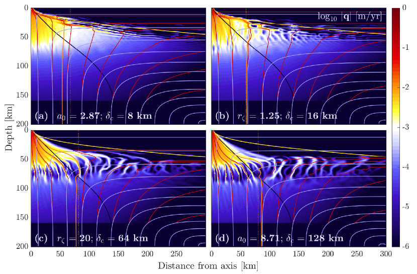
Figure S2: Darcy flux magnitude $|\mathbf{q}|$ at $t=10$ Myr for simulations with compaction lengths of (a) 8 km, (b) 16 km, (c) 64 km, and (d) 128 km. Streamlines for melt (red) and solid (blue) flow, outline of primary upwelling domain (black), and melt focusing domain (orange), with $x_{e}$ (dotted) for comparison. At small compaction length melt streamlines are dominantly vertical or along inclined plane of LAB. Melt streamlines are increasingly bent away from the thermal boundary layer with growing compaction length. Channels are more pronounced at high compaction lengths.

The striking anti-correlation between focusing of MORB and hMORB in Fig. 4(g)–(h) shows the control of melt extraction pathways on extracted melt compositions. With increasing compaction length, active focusing becomes more important relative to passive focusing. Melt streamlines curve away from the vertical toward the ridge axis at greater depth (c.f. Suppl. Fig. S2). Melt is transported away from the thermal boundary layer and hence interaction with the cooler lithosphere is minimised. Active focusing thus leads to less volatile enrichment by fractional crystallisation as compared to passive focusing. Less enrichment is also expected for other incompatible elements in the melt. Some of the compositional diversity of extracted melt may thus be attributed to different pathways of melt extraction, rather than to variations in source composition or degree of melting.

3.2 Crustal thickness

Predicted crustal thickness is an important model metric that can be compared with observations (see Appendix C). Figure 5(a)–(e) shows the time averaged crustal thickness $\langle H_{c}\rangle$ plotted against the same parameters as in Fig. 4 (full time-series of $H_{c}$ in Suppl. Fig. S4). Crustal thickness as a function of spreading rate shows the characteristic saturation towards fast spreading ridges. For comparison, MOR crustal thickness data obtained from seismics and rare-Earth-element inversions (White et al., 2001) are plotted alongside simulation results. Motivated by the variation with spreading rate, we fit the simulation output and observational data with a log-cubic functions. The results are shown as dotted and dashed lines, respectively, in panel (a). Qualitatively, the simulation results follow the same trend as the observational data. However, our reference model result of $\sim$12 km crustal thickness is considerably higher than the observed $\sim$7 km. We will return to this point below.

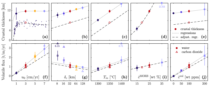
Figure 5: Time-averaged crustal thickness $\langle H_{c}\rangle$ and volatile extraction rate $\langle q^{\mathrm{vol}}_{\mathrm{focus}}\rangle$ as function of parameter values. Results for $\langle H_{c}\rangle$ (circles) are plotted as a function of: (a) half- spreading rate; (b) compaction length; (c) potential temperature; (d) fertility; (e) volatile content. Bars indicate $\pm 2\sigma$. Dots in (a) are data from White et al. (2001). (f)–(j) show $\langle q^{\mathrm{vol}}_{\mathrm{focus}}\rangle$ for H₂O (squares), and CO₂ (triangles) as function of same parameter variations. Dotted lines are regressions of the simulation output; dashed lines are adjusted regressions to fit crustal thickness data; open symbols not included in regressions.

Crustal thickness is shown to correlate with compaction length in Figure 5(b). This is a consequence of more efficient melt focussing with increasing compaction length. A log-linear regression of the simulation output shows that a doubling of compaction length leads to a $\sim$0.7 km increase in crustal thickness. Crustal thickness also increases significantly with higher potential temperature in panel (c), and mantle fertility in panel (d). A linear regression of the results with temperature and a quadratic regression with fertility show that 1 km of additional crust are produced by a $\sim$16 ^∘C increase in $T_{m}$ or by a $\sim$1.5 wt% increase in $\bar{c}^{\mathrm{MORB}}$, holding everything else constant.

Whereas these trends follow expectations from previous analyses, the absolute melt production in our models is above observational constraints. We use the regression from panel (d) to calculate the fertility reduction required to shift the fertility in the reference model down such that the misfit with observational constraints is reduced. The required shift in $\bar{c}^{\mathrm{MORB}}$ is $-6$ wt%. To check this shift, we include an additional simulation with the MORB component concentration reduced to 19 wt%. The result is shown as open circles in panels (a)–(e); as expected, the adjusted crustal thickness is $\sim$7 km. Adjusted regression curves for other parameters are shown as dashed lines.

The sensitivity of crustal thickness to mantle volatile content is relatively small: 1 km of additional crust is produced by an increase of $\sim$140 wt ppm each of H₂O and CO₂ (more than doubling the reference value). In contrast, the temporal variability of crustal thickness is highly sensitive to volatile content. It follows that variability of magma supply at the ridge axis is not necessarily diagnostic of source heterogeneity in mantle fertility or volatiles — all simulations are seeded with the identical mantle heterogeneity. Rather, the temporal variability seen here is a result of channelised melt transport and its associated intermittency in space and time.

3.3 Volatile extraction

Rates of H₂O and CO₂ extraction by focused magma at the axis are given by $q^{\mathrm{H_{2}O}}_{\mathrm{focus}}$, and $q^{\mathrm{CO_{2}}}_{\mathrm{focus}}$ (see Appendix C). For H₂O, the extraction rate is interpreted as water supplied to the oceanic crust. Most of this water will remain contained within the crust but most of the CO₂ focused to the ridge is degassed from the shallow magmatic system into the ocean–atmosphere reservoir.

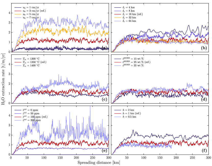
Figure S5: Time series of H₂O extraction rate for all parameter choices. Results plotted against spreading distance. Time averages extracted over interval from 180–300 km. The resolution tests in h show that water extraction in the reference case is well resolved at reference conditions.

Fig. 5(f)–(j) shows time-averaged volatile extraction rates plotted against mantle parameters (full time-series of extraction rates in Suppl. Figs S5–S6). Under most conditions, H₂O and CO₂ extraction rates are nearly identical. As discussed above, volatile dilution by shallow, high-degree melting precludes their fractionation. Furthermore we find that the instances where the behaviour of CO₂ and H₂O differ are best explained by errors associated with insufficient numerical resolution. Simulations with $\delta_{c}<32$ km have significant mass conservation errors for the incompatible components. Hence cMORB is more strongly affected while hMORB remains mostly well resolved. MORB and dunite components are not affected (see Suppl. Figs S5(f) & S6(f) for resolution test results). We therefore proceed with discussion of the hMORB component and assert that these results are a meaningful proxy for CO₂ extraction.

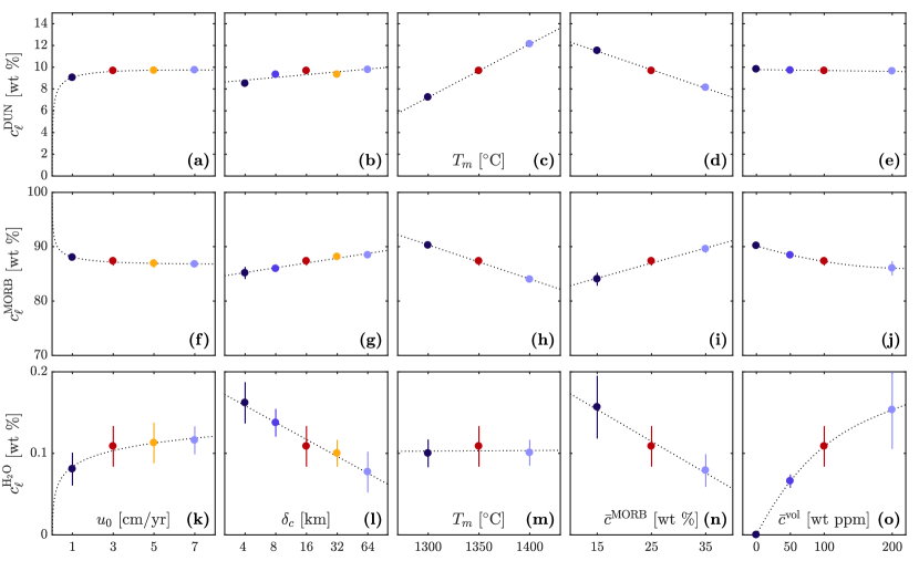
Figure S7: Component concentrations in melt focused to the ridge axis. Time averaged concentrations of dunite (a)– (e), MORB (f)–(j), and H₂O (k)– (o), with bars for $\pm 2\sigma$ variability, shown as a function of: half-spreading rate, compaction length, potential temperature, fertility, and volatile content. Dotted lines are regressions of simulation outputs.

Volatile extraction rates increase linearly with half-spreading rate in panel (f). At reference parameters the extraction rate is $\sim$1200 kg/m/yr. In the model with shifted reference fertility it is reduced to $\sim$950 kg/m/yr (open square). A linear regression through the origin and this shifted reference rate (dashed line) has an increase in volatile extraction rate of $\sim$320 kg/m/yr for every 1 cm/yr increase in $u_{0}$. This sensitivity is comparable to idealised models of MOR carbon degassing by Burley and Katz (2015). The correlation with spreading rate is the result of increased melt production, while volatile concentration in the magma remains relatively stable (c.f. time-averaged melt compositions in Suppl. Fig. S7).

The decrease of extraction rates with increasing compaction length in panel (g) is, again, associated with the shift toward more active focussing. As melt is diverted away from the sub-lithospheric crystallisation front, deep fractional crystallisation and the consequent enrichment of incompatibles is reduced. Results at small $\delta_{c}$ suggest insufficient numerical resolution. A log-linear regression of the well-resolved results at higher $\delta_{c}$ has a drop in volatile extraction rate of $\sim$110 kg/m/yr for a doubling of $\delta_{c}$. An increase in mantle temperature in panel (h) and fertility in panel (i) both lead to a moderate increase in volatile extraction, as the deepening and widening of the volatile-free melting regime allows some more distal volatile-rich melt to be focused. Linear regressions of these results show that a rate increase of 100 kg/m/yr is produced by either a temperature increase of $\sim$14 ^∘C or an additional $\sim$3.4 wt% mantle fertility.

Volatile extraction at the ridge axis is proportional to the mantle volatile content in panel (j). Regression through the origin and the data point from the adjusted fertility reference simulation shows that an additional 10 wt ppm volatiles in the mantle gives an increase of $\sim$95 kg/m/yr in ridge extraction rate. The signature of increased channelised transport at higher volatile contents is expressed by higher variability of extraction rates. The relative amplitude of these variations is up to 50%. Again, this variability is not caused by source heterogeneity or variable degrees of melting. Rather it is the signature of reactive melt transport in the asthenosphere.

4 Simulation-based estimates of global MOR volatile output

4.1 Distribution along the global MOR system

The simulations presented here can provide a novel perspective on the globally integrated MOR output. Using the regressions of simulation output in Fig. 5 we interpolate crustal thickness and volatile extraction rate to conditions found along the global MOR system. However, in reading the results, one should bear in mind the limitations of this method: each regression curve was obtained for an isolated parameter variation in a complex, non-linear system; the natural system may be characterised by significant covariation between parameters. Despite this limitation, we expect to gain insights into possible global patterns as well as globally integrated magnitudes of MOR output.

Conditions along the global MOR system are available from a catalogue of ridge segments composed by Gale et al. (2014), which gives the location, length, and spreading rate of each segment. Dalton et al. (2014) obtained estimates of potential temperature beneath segments on the basis of inversion of observed ridge depth, S-wave speed, and MORB geochemistry. We use those estimates to assign mantle temperature for each ridge segment in the Gale et al. (2014) catalogue. We shift the temperatures by -25 ^∘C to align their average temperature to our reference temperature of 1350 ^∘C. For ridge segments not included in Dalton et al. (2014), we interpolate between the nearest available constraint and 1350 ^∘C. Figure 6(a)–(b) shows half- spreading rate and mantle potential temperature plotted on the mid-point coordinates of each ridge segment in the combined catalogue.

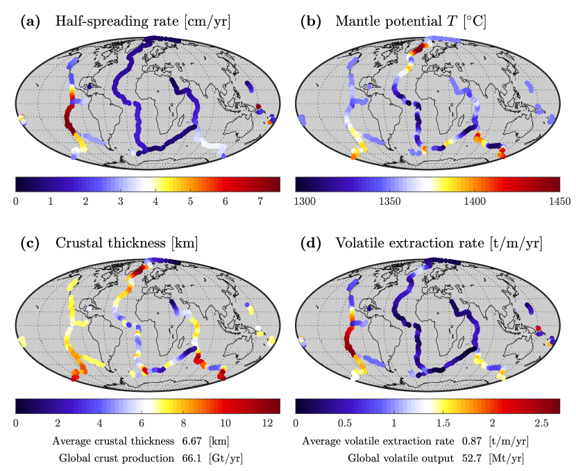
Figure 6: MOR magmatic flux estimates for global ridge system with $\bar{c}^{\mathrm{H_{2}O}}=100$ ppm: (a) Half-spreading rates taken from Gale et al. (2014); (b) Mantle potential temperature extrapolated from Dalton et al. (2014); (c) Crustal thickness, and (d) volatile extraction rate calculated from regressions of simulation outputs. Each data point represents one ridge segment in Gale et al. (2014) catalogue.

Global average values for mantle fertility, volatile content and compaction length are approximately known. Regions of increased volatile content are typically linked to nearby hotspots (e.g., Azores (Asimow et al., 2004)). Yet, emerging information about these variations along the ridge system is still sparse (Le Voyer et al., 2017). Therefore, we will investigate the range of $100\leq\bar{c}^{\mathrm{H_{2}O}}\leq 200$ ppm, along with reference values for $\delta_{c}=32$ km, $\bar{c}^{\mathrm{MORB}}=19$ wt% (the adjusted value). We can now use the adjusted regressions in Fig. 5 to compute crustal thickness and volatile extraction rate for each segment in the catalogue.

The predicted global distribution for $\bar{c}^{\mathrm{H_{2}O}}=100$ ppm, is shown in Fig. 6(c)–(d). The pattern of crustal thickness in panel (c) mostly follows the pattern of mantle temperature from Dalton et al. (2014). The thickest crust is found in regions influenced by hot-spots, most pronounced beneath Iceland. There crustal thickness exceeds 12 km. The global average crustal thickness is 6.67 km. The lowest values are found at the eastern end of the Southwest Indian Ridge, at $<2$ km. The distribution of volatile extraction rate, in contrast, shows a strong dependence on spreading rate, with only a weak influence of mantle temperature. The highest volatile extraction rates of $>2.5$ t/m/yr occur along the East Pacific Rise. The global average rate is 0.87 t/m/yr. For cool, slow-spreading ridge sections such as parts of the Mid-Atlantic and Southwest Indian Ridges, values are $<0.25$ t/m/yr.

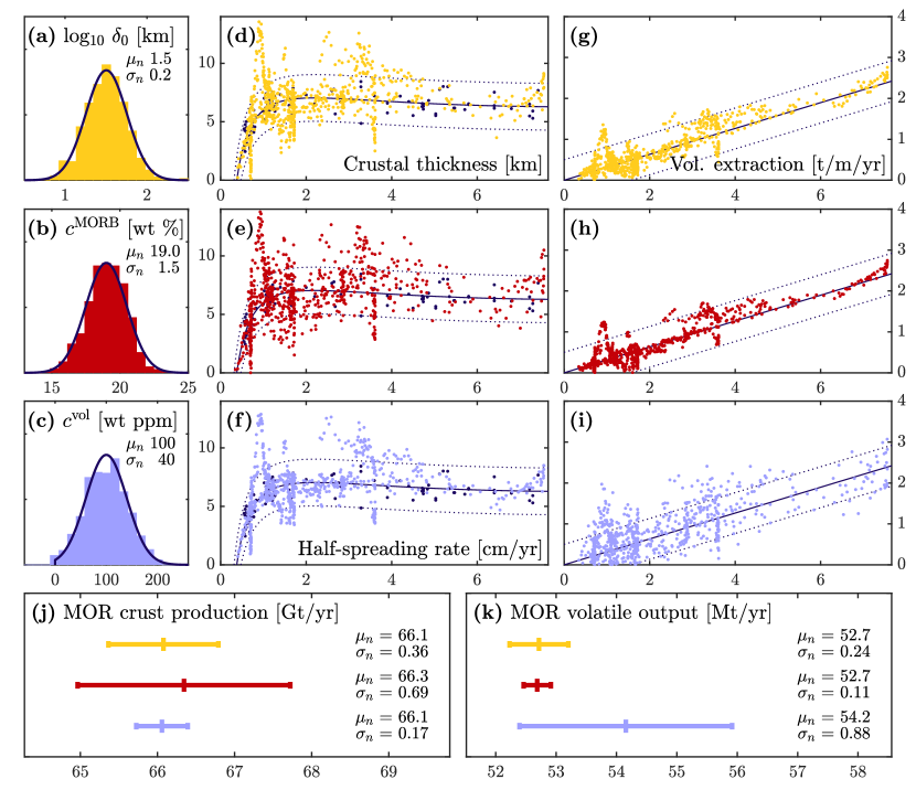
Figure 7: Globally integrated MOR magmatic flux estimates. Parameter distributions (line) and example histogram (bars) for segment-wise sampling of (a) compaction length, (b) mantle fertility, and (c), volatile content. Crustal thickness (d)–(f), and volatile extraction rate (g)-(h) calculated from fitting functions for example parameter distribution. White et al. (2001) data points for comparison (black); Lines show adjusted fitting functions for crustal thickness with best fit parameters (solid), and $\pm$ 2 km variation (dotted), and for extraction rate with best fit parameters (solid) and $\pm$ 0.5 t/m yr variation (dotted). Normal distributions fitted to population of globally integrated output from 1383 sampling instances (j)–(k). Colours denote individually sampled problem parameters.

4.2 Range of global MOR output

Globally integrated MOR output can be obtained from the distributions above. For crust production, we multiply crustal thickness by $2u_{0}\rho_{c}$ and integrate over the length of ridge segments. The resulting projection of global crust production is 66.1 Gt/yr— equivalent to 22 km³/yr. Similarly, integrating the volatile extraction rate over the length of ridge segments after Burley and Katz (2015) predicts the global MOR volatile output to be 52.7 Mt/yr of H₂O and CO₂ each for reference volatile content. Repeating the global calculation above for a mean mantle volatile content of 200 ppm gives a global volatile output of 110.2 Mt/yr. The corresponding global crust production is 73.1 Gt/yr (24 km³/yr). The average volatile concentration in (undegassed, undifferentiated) focused melt is calculated by dividing the global volatile extraction by the crust production rate. The calculated values are 0.08 and 0.15 wt% for 100 and 200 ppm H₂O and CO₂ in the mantle. According to our calculations, measured H₂O (0.13–0.77 wt%) and reconstructed CO₂ (0.066–5.75 wt%) concentrations in MORB by Cartigny et al. (2008) would map back to global mean concentrations of $>$170 ppm H₂O and $>$80 ppm CO₂; the upper limits would map to values well above 1000 ppm.

In addition to these leading-order global figures, we estimate the uncertainty of global MOR output arising from uncertainty in geographic, segment-wise variations of parameters that are not listed in the above catalogue. To this end we assume that mantle fertility, volatile content and compaction length are not constant in the upper mantle, but are distributed over a plausible range. Black curves in Figure 7 (a)–(c) show distributions of compaction length, fertility, and volatile content that are proposed to represent variation in the asthenosphere beneath the ridge system. Each distribution is centred around the reference values above. We assume compaction length has a log-normal distribution across a range of $\sim$10–100 km ($\mu_{n}\pm 2\sigma_{n}$); fertility is normally distributed with a range of $\sim$16–22 wt%; volatile content is normally distributed with a range of $\sim$20–180 wt ppm (truncated at zero).

A population of instances of global MOR output is produced by repeating the following three steps. First, one of the three parameters is randomly sampled according to its distribution to obtain a value for each ridge segment. A histogram of a sample is shown for each parameter in Fig. 7(a)–(c). Second, segment-wise crustal thickness and volatile extraction rate are computed from regressions as above. Calculated values for sampled parameter sets in panels (a)–(c) are plotted against spreading rate in panels (d)–(i). Third, instances of globally integrated MOR output are calculated by integrating over the length of ridge segments. These three steps are repeated separately for each of these three parameters until each parameter-specific population of instances is fitted by a normal distribution to a relative tolerance of $10^{-3}$.

The populations for crust production and volatile output obtained from $\gtrsim 10^{3}$ instances of statistically sampled parameter sets are shown in Fig. 7(j)–(k). The ranges of outcomes are shown as $\mu_{n}\pm 2\sigma_{n}$. Global crustal production is most sensitive to mantle fertility variations with a range of 65–68 Gt/yr. Global volatile extraction rate is most sensitive to mantle volatile content with a range of 52–56 Mt/yr. Variations in compaction length and mantle fertility have second-order effects on the range of volatile output.

These projected values of global volatile export from the mantle fall within the range of previous estimates, particularly in comparison to previous estimates of CO₂ emissions from MOR degassing (Resing et al., 2004; Cartigny et al., 2008; Dasgupta and Hirschmann, 2010; Kelemen and Manning, 2015). However, limitations of the present method should moderate our confidence in the produced estimates of MOR volatile output. The validity of the physical model and its numerical implementation is limited. For example, a more realistic rheology depending on stress and dynamically evolving grain size could have important effects on melt segregation (Turner et al., 2015); the model of mantle melting is based on simplified thermodynamics that are, at best, a crude approximation of full mantle petrogenesis; and the simulations skirt the limits of spatial resolution, introducing potentially disruptive mass conservations errors for incompatible species. Furthermore, using single-parameter regressions of simulation output neglects possible non-linear effects of parameter co-variations; polynomial degrees for regressions were chosen for convenience, not consistency with physical processes.

Nevertheless, the present method produces estimates of MOR volatile output that are consistent with dynamic simulations taking into account conservation of mass, momentum and energy. The models are calibrated to reproduce accepted features of MORB petrogenesis to leading order. Model parameters are tuned with the most recent observational constraints on the global MOR system, where available. The present estimates of global MOR volatile output are consistent with available constraints on extraction processes. Our method estimates MOR output for a range of global mean mantle properties and it quantifies the uncertainty associated with plausible regional distributions around reference conditions.

5 Deep volatiles and the LAB

From the above it is evident that not all melt produced beneath a MOR is focused to the ridge axis. Instead, a significant fraction of the deep, volatile-rich melt is transported towards the oceanic LAB. As seen in Fig. 1, this transport creates remnants of reactive channels bent away from the axis through plate motion. Over time such channels become stagnant sub-horizontal melt bodies stacked along the LAB. This feature of our results could help explain the sharp negative shear-wave velocity contrasts identified along the oceanic LAB in recent studies (Kawakatsu et al., 2009; Schmerr, 2012; Stern et al., 2015). We find that such melt lenses, which contain melt fractions of 5–25% (some up to 50%), are typically located along the 1200 ^∘C isotherm. Some of this stalling melt could be further extracted by dike propagation (e.g. Havlin et al., 2013), an effect not currently included in our models. With ongoing crystallisation, volatiles are enriched in the fractionated liquid; the oceanic LAB is metasomatised by these volatile-rich liquids. In contrast to simpler models (e.g. Plank and Langmuir, 1992; Hirth and Kohlstedt, 1996; Asimow and Langmuir, 2003), the volatile content with depth beneath the ocean floor (i.e., the RMC) does not reflect either a fractional or batch melting residue. Instead, the depth profile of volatiles is a result of complex transport processes. In particular, channelised melt transport leads to a heterogeneous distribution of volatiles along the LAB as it moves away from the ridge axis.

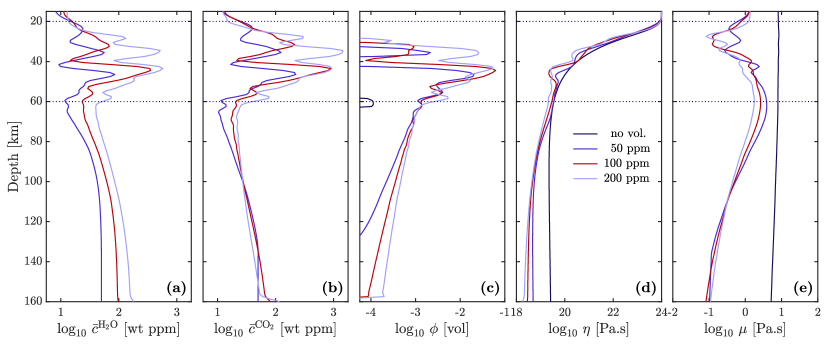
Figure 8: Averaged depth profiles of volatile and melt content, and rheology along far flank of ridge. Depth profiles obtained by horizontal averaging over interval from 200–300 km distance from axis, and triangular moving average along profile. Water and carbon dioxide bulk concentrations (a) & (b); melt fraction (c); rock viscosity (d); melt viscosity (e). Given for simulations with 0 (black), 50 (blue), 100 (red), 200 (light blue) wt ppm initial volatile content. Where no melt present, melt viscosity is found from fractional melt composition.

Figure 8 shows depth profiles produced by horizontally averaging simulation results in the interval from 180 to 300 km from the axis (6–10 Myr plate age). These profiles are then filtered with a vertical moving-average to emphasise structures larger than $\gtrsim$5 km. Figure 8 shows results from simulations with various volatile contents. Moving upwards from 160 to 60 km depth, both H₂O and CO₂ follow a trend of depletion. Above is found an enriched region from 60 to 20 km depth. The enrichment is layered and reaches concentrations up to 1000 ppm; it is stronger for CO₂ than for H₂O, which indicates fractional crystallisation of accumulated low-degree melts. This layered band of metasomatised mantle coincides with the top boundary of the partially molten domain. Below 60 km depth, melt is stable at low fractions of 0.01–0.1%. Along the thermal LAB at $\sim$60–50 km depth, melt is accumulated into decompaction layers with horizontal averages upwards of 1% melt. Some remains of crystallising melt are found to a depth of 30 km. It is conceivable that such melt layers are a source of off-axis seamount volcanism.

Volatile enrichment along the LAB has consequences for rock viscosity, as shown in Fig. 8(d). Viscosity is reduced by water; a gradual increase in viscosity above the base of the melting regime reflects volatile depletion by melt extraction. Along the band of metasomatism, however, rehydration of the solid creates layers with up to an order of magnitude reduction of viscosity. These represent a structural heterogeneity at the base of the lithosphere. Such rheological structure could help explain the sharp decrease in shear- wave speed observed along the oceanic LAB (see Olugboji et al., 2016, and references therein). Our results support the current hypothesis that these signals reflect the presence of partial melt and/or hydrated material along the LAB. Furthermore, a metasomatised oceanic lithosphere has recently been evoked as the potential source of enriched alkaline ocean island basalts (Workman et al., 2004; Pilet et al., 2011) and highly alkaline petit-spot volcanism (Hirano, 2011).

Lastly, the depth profiles of magma viscosity in Fig. 8(e) show a clear signal of lubrication by volatile enrichment. The signal is seen in deep primitive as well as in shallow fractionated melt. This viscosity variation promotes melt segregation from the mantle residue even at small melt fractions $<0.1$ wt%. An appropriate liquid viscosity model with volatile content is thus crucial for understanding the transport of volatiles in the mantle beneath mid-ocean ridges.

6 Summary and conclusions

We present dynamic models of thermochemically coupled magma/mantle dynamics with volatiles beneath a mid-ocean ridge. The presence of volatiles in low concentrations in the mantle source causes deep, low-degree, volatile-rich melting. Due to the corrosive effect of volatile-rich melt on silicates with decreasing pressure, the flux of deep melt into the volatile-free melting regime triggers reactive channelisation. We find that melt focussing to the axis is not extended by channelised flow. Rather, channelling introduces spatial and temporal heterogeneity in flux and melt composition at the ridge axis.

We investigate volatile extraction from the asthenosphere across a range of parameters including spreading rate, compaction length, mantle temperature, fertility and volatile content. Volatile extraction depends on the rate of melt delivery to the axis, as well as the concentration of volatiles therein. The efficiency of melt focusing increases with compaction length, mantle temperature and fertility. The concentration of volatiles in that melt depends on the melt extraction pathways and, in particular, whether they approach the thermal boundary layer along the LAB, where fractional crystallisation leads to volatile enrichment.

We calculate crustal thickness and volatile extraction rates for individual ridge segments in a global catalogue using regressions of simulation outputs and crustal thickness data. The resulting distribution of projected crustal thickness is mainly controlled by mantle temperature, whereas the distribution of volatile extraction rate dominantly reflects spreading rate. Global integration gives values of 66–73 Gt/yr (22–24 km³/yr) for global crust production and a global volatile output of 53–110 Mt/yr, corresponding to mantle volatile contents of 100–200 ppm. The uncertainty of these estimates relating to the uncertain distribution of mantle conditions along the global ridge system is assessed using statistical sampling from plausible distributions of compaction length, mantle fertility and volatile content. The resulting range of uncertainty for parameters distributed around reference mantle conditions is 65–68 Gt/yr for crust production and 50–55 Mt/yr for volatile output.

Finally, and in contrast to Asimow and Langmuir (2003), our models suggest that up to half of dissolved volatiles that cross into the melting regime are not focused to the axis, but are instead extracted towards the flanks of the ridge, where they metasomatise the mantle along the LAB. The resulting rheological heterogeneity caused by water-weakening of mantle rock could explain seismic signals interpreted as evidence of the oceanic LAB depth. Our results show bands of metasomatised rock at a depth range of 20–60 km at spreading ages of 6–10 Myr, consistent with LAB-related signals in seismic studies.

Acknowledgements

The research leading to these results has received funding from the European Research Council under the European Union’s Seventh Framework Programme (FP7/2007–2013)/ERC grant agreement number 279925. Hirschmann acknowledges support from NSF grant EAR1426772. The authors thank the Isaac Newton Institute for Mathematical Sciences for its hospitality during the programme Melt in the Mantle which was supported by EPSRC Grant Number EP/K032208/1. Katz is grateful for the support of the Leverhulme Trust. The authors further thank the Geophysical Fluid Dynamics group for access to the BRUTUS cluster at ETH Zurich, Switzerland. Thanks to R. White, C. Dalton, and A. Gale for making their data available.

References

Appendix A R_DMC: Equilibrium and reaction model

The following is a brief summary of the R_DMC method, which provides a model of thermodynamic equilibrium and linear kinetic reactions for multi-component compositional models of mantle petrogenesis. A detailed description of the method is found in Keller and Katz (2016). The method provides closure conditions for reaction rates $\Gamma^{i}$ needed to couple conservation equations for energy, phase and component mass in a multi-phase, multi- component reactive flow model. It consists of the following four steps:

(i) Determine partition coefficients $K^{i}$ for each effective component ($i=1,...,n$) at given $P,T$-conditions. The partition coefficients are functions of $T$ and $P$, following a simplified form of ideal solution theory (Rudge et al., 2011). Effective components are chosen to approximate the petrological processes of interest within a framework of tractable complexity. Here, we represent mantle melting with four effective components ($n=4$): dunite and mid-ocean ridge basalt as the residual and product of volatile-free mantle melting, and hydrated and carbonated basalt as the products of hydrated and carbonated silicate melting at depth.

(ii) For a given bulk composition $\bar{c}^{i}=\phi c_{\ell}^{i}+(1-\phi)c_{s}^{i}$, determine the unique melt fraction $\phi^{\mathrm{eq}}$ for which all components are in equilibrium according to $K^{i}$. We do so by combining the lever rules for each component, partitioned between the phases according to $K^{i}$, with the constraint that all component concentrations in each phase must sum to unity. Thus we formulate the implicit statement

$$\sum\limits_{i=1}^{n}\dfrac{\bar{c}^{i}}{\phi^{\mathrm{eq}}/K^{i}+(1-\phi^{\mathrm{eq}})}-\sum\limits_{i=1}^{n}\dfrac{\bar{c}^{i}}{\phi^{\mathrm{eq}}+(1-\phi^{\mathrm{eq}})K^{i}}=0\>,$$ (3)

which we solve numerically for $\phi^{\mathrm{eq}}$.

(iii) Find the equilibrium phase compositions $c_{s}^{i,\mathrm{eq}}$ (solid), $c_{\ell}^{i,\mathrm{eq}}$ (liquid) at equilibrium melt fraction $\phi^{\mathrm{eq}}$ by lever rule

$$c_{s}^{i,\mathrm{eq}} =\dfrac{\bar{c}^{i}}{\phi^{\mathrm{eq}}/K^{i}+(1-\phi^{\mathrm{eq}})},$$ (4)

$$c_{\ell}^{i,\mathrm{eq}} =\dfrac{\bar{c}^{i}}{\phi^{\mathrm{eq}}+(1-\phi^{\mathrm{eq}})K^{i}}\>.$$

(iv) Use linear kinetic constitutive laws to determine equilibration reaction rates $\Gamma^{i}$ driven by compositional disequilibria

$$\Gamma^{i}=\mathcal{R}_{\Gamma}(\phi^{\mathrm{eq}}c_{\ell}^{i,\mathrm{eq}}-\phi c_{\ell}^{i})\>.$$ (5)

The linear kinetic rate factor $\mathcal{R}_{\Gamma}=\rho_{0}/\tau_{\Gamma}$ ensures that equilibration is applied over a specified reaction time scale $\tau_{\Gamma}$, with $\rho_{0}$ the reference solid density. The net melting rate $\Gamma$ is the sum of all component rates $\Gamma^{i}$. These reaction rates drive the system toward chemical equilibrium.

Appendix B Rheology with volatiles

The viscosity of mantle rock is taken as diffusion creep of olivine with melt- and water-weakening (Hirth and Kohlstedt, 2003; Mei et al., 2002). Constitutive laws for shear and compaction viscosities $\eta,~{}\zeta$ are written in standard form as a function of lithostatic pressure $P$, temperature $T$, grain size $a_{0}$ (assumed constant and uniform), water content $C_{H}$, and melt fraction $\phi$:

$$\eta^{\mathrm{dry}} =A_{0}^{\mathrm{dry}}a_{0}^{3}\exp\left(\dfrac{E_{a}+PV_{a}}{RT}-\alpha\phi\right)\>,$$ (6a)

$$\eta^{\mathrm{wet}} =A_{0}^{\mathrm{wet}}C_{H}^{-1}a_{0}^{3}\exp\left(\dfrac{E_{a}+PV_{a}}{RT}-\alpha\phi\right)\>,$$ (6b)

$$\eta =\min(\eta^{\mathrm{dry}},\eta^{\mathrm{wet}})\>,$$ (6c)

$$\zeta =r_{\zeta}\>\eta\>\phi^{-1}.$$ (6d)

The parameter $r_{\zeta}$ represents the poorly constrained ratio of compaction to shear viscosity. $C_{H}$ is obtained by converting dynamically calculated water concentrations in the solid phase to the appropriate units (1 ppm H₂O equals 5.4 H/($10^{6}$ Si), c.f. Hirth and Kohlstedt (1996)).

The viscosity of the volatile-bearing silicate melt is taken to depend on composition: weakening with increasing concentration of H₂O and CO₂, stiffening with increasing dissolved silica. The consitutive law is log-linear:

$$\mu=\mu_{0}\prod\limits_{i=1}^{n}\lambda^{i}c_{\ell}^{i}\>.$$ (7)

Factors $\lambda^{i}$ are chosen such that melt viscosity varies between 0.01 Pa-s for a volatile-rich melt to 10 Pa-s for a volatile-poor melt. Permeability depends on grain size and melt fraction according to the Kozeny-Carman relation,

$$K=\dfrac{a_{0}^{2}}{100}\dfrac{\phi^{3}}{(1-\phi)^{2}}.$$ (8)

With the above constitutive laws the compaction length (1) depends on temperature, melt fraction and composition, which are features of the solution. However, $\delta_{c}$ can be independently varied by changing either $r_{\zeta}$ or $a_{0}$. From equation (1), with (6) and (8), we find that $\delta_{c}$ scales as $\sqrt{r_{\zeta}}$ and $a_{0}^{5/2}$. With reference values of $r_{\zeta}=5$ and $a_{0}=5$ mm, the compaction length is 32 km. This value is calculated at conditions representative of the shallow partially molten asthenosphere beneath the ridge, with $\phi=0.01$, $\eta=4\times 10^{19}$ Pa-s and $\mu=5$ Pa-s. The permeability under these conditions is $2.6\times 10^{-13}$ m². The values of $\delta_{c}=16$ and 64 km in the parameter study above arise from $r_{\zeta}$ of 1.25 and 20 respectively, and values of $\delta_{c}=8$ and 128 km are obtained from $a_{0}$ of 2.87 and 8.71 mm respectively.

Table A1 contains a list of model parameters and their reference values. Parameters not listed there are the same as in Table 1 of Keller and Katz (2016).

Table A1: Simulation parameters, definitions, and reference values

Depth of domain	$D$	km	200
Width of domain	$W$	km	300
Mantle density	$\rho_{0}$	kg/m3	3200
Crustal density	$\rho_{c}$	kg/m3	3000
Rock to melt density contrast	$\Delta\rho$	kg/m3	500
Half-spreading rate	$u_{0}$	cm/yr	3
Dry pre-exponential factor	$A_{0}^{\mathrm{dry}}$	Pa-s/m3	1.11$\times 10^{14}$
Wet pre-exponential factor	$A_{0}^{\mathrm{wet}}$	Pa-s (106 H/Si)/m3	6.67$\times 10^{15}$
Activation energy	$E_{a}$	J/mol	3.75$\times 10^{5}$
Activation volume	$V_{a}$	m3/mol	4$\times 10^{-6}$
Universal gas constant	$R$	J/mol/K	8.314
Rock viscosity melt-weakening factor	$\alpha$	Pa-s	30
Compaction to shear viscosity ratio	$r_{\zeta}$	-	5
Melt viscosity constant	$\mu_{0}$	Pa-s	1
Melt viscosity compositional factors	$\lambda^{i}$	-	[1,10,0.1,0.01]
Grain size constant	$a_{0}$	m	5$\times 10^{-3}$

Appendix C Mass transfer rates from simulation output

The following three rates of mass transfer per unit length of ridge axis are recorded to quantify melt production and focusing in simulation results. They have units of kg yr^-1m^-1.

First, $q_{\mathrm{base}}^{i}$ is the integral of component mass advected across the base of the melting regime,

$$q_{\mathrm{base}}^{i} =\int\limits_{0}^{W}2\rho_{0}(1-\phi)c_{s}^{i}w_{s}~{}\textrm{d}x~{}\mid_{z=z_{\mathrm{sol}}}\>,$$ (9)

where $W$ is the width of the domain, $w_{s}$ is the solid upwelling rate and $c_{s}^{i}$ denote the mass concentrations of chemical components ($i\in\{\text{DUN, MORB, hMORB, cMORB}\}$). The factor two accounts for the symmetrical other half of the ridge system. The total mantle inflow rate is obtained from the sum of component-wise rates, $q_{\mathrm{base}}=\sum\limits_{i=1}^{n}q_{\mathrm{base}}^{i}$.

Second, $q_{\mathrm{melt}}^{i}$ is the integral of positive component-wise melting rates across the model domain,

$$q_{\mathrm{melt}}^{i} =\int\limits_{0}^{W}\int\limits_{0}^{z_{\mathrm{sol}}}2\Gamma^{i}_{+}~{}\textrm{d}x~{}\textrm{d}y\>,$$ (10)

where

$$\Gamma^{i}_{+}=\begin{cases}\Gamma^{i}&\text{if $\Gamma^{i}>0$}\\ 0&\text{otherwise}\>\>.\end{cases}$$

The total melt production rate is obtained by summing over the components, $q_{\mathrm{melt}}=\sum\limits_{i=1}^{n}q_{\mathrm{melt}}^{i}$.

And third, $q_{\mathrm{focus}}^{i}$ is the integral of component-wise melt focused to the ridge axis,

$$q_{\mathrm{focus}}^{i} =\int_{0}^{W}2\rho_{0}\phi c_{\ell}^{i}w_{\ell}~{}\textrm{d}x~{}\mid_{z=d}\>,$$ (11)

where $d=8$ km is the depth at the base of the imposed melt extraction zone in the axis and $w_{\ell}$ is the vertical rate of melt flow. The total melt focusing rate is $q_{\mathrm{focus}}=\sum\limits_{i=1}^{n}q_{\mathrm{focus}}^{i}$.

The predicted crustal thickness is calculated from the ratio of melt focusing and plate spreading rates:

$$H_{c}=q_{\mathrm{focus}}/(2\rho_{c}u_{0})\>,$$ (12)

with the density of oceanic crust $\rho_{c}=3000$ kg/m³.

Finally, extraction rates for H₂O and CO₂ are calculated by multiplying the focusing rates of the volatile-bearing components by their constant volatile contents. Hence we have $q^{\mathrm{H_{2}O}}_{\mathrm{focus}}=0.05\times q^{\mathrm{hMORB}}_{\mathrm{focus}}$, and $q^{\mathrm{CO_{2}}}_{\mathrm{focus}}=0.20\times q^{\mathrm{cMORB}}_{\mathrm{focus}}.$

Supplementary Material to: ”Volatiles beneath mid-ocean ridges: deep melting, channelised transport, focusing, and metasomatism”

by Tobias Keller, Richard F. Katz, and Marc M. Hirschmann.

The Supplementary Material below provides the Supplementary Table S1 and seven Supplementary Figures, S1–S7, as referenced in the article.

Table S1: Parameter variations for simulation runs

Run ID	$u_{0}$	$T_{m}$	$c^{\mathrm{morb}}$	$c^{\mathrm{vol}}$	$r_{\zeta}$	$a_{0}$	$A_{p}^{morb}$	$A_{p}^{\mathrm{vol}}$	$\eta(c_{H})$	$\mu(c^{i})$	$\eta(\phi)$	$D$	$D_{\mathrm{sol}}^{\mathrm{max}}$	$h$	Comments
	cm/yr	∘C	wt %	wt ppm	1	mm	%	%	-	-	-	km	km	km	units
morb0	-	-	-	-	-	-	0	-	-	-	-	-	-	-	high pert. ampl.
morb1	3	1350	25	100	5	5	10	0	on	on	on	200	160	1	heterogeneous ref.
morb2	-	-	-	-	-	-	50	-	-	-	-	-	-	-	high pert. ampl.
morb3	1	-	-	-	-	-	-	-	-	-	-	-	-	-	slow-spreading
morb4	5	-	-	-	-	-	-	-	-	-	-	-	-	-	fast-spreading
morb25	7	-	-	-	-	-	-	-	-	-	-	-	-	-	fastest-spreading
morb5	-	1300	-	-	-	-	-	-	-	-	-	-	-	-	low pot. T
morb6	-	1400	-	-	-	-	-	-	-	-	-	-	-	-	high pot. T
morb7	-	-	15	-	-	-	-	-	-	-	-	-	-	-	low fertility
morb8	-	-	35	-	-	-	-	-	-	-	-	-	-	-	high fertility
morb9	-	-	-	0	-	-	-	-	-	-	-	-	-	-	no volatiles
morb22	-	-	-	50	-	-	-	-	-	-	-	-	-	-	low volatiles
morb10	-	-	-	200	-	-	-	-	-	-	-	-	-	-	high volatiles
morb11	-	-	-	100 (H)	-	-	-	-	-	-	-	-	-	-	water only
morb12	-	-	-	100 (C)	-	-	-	-	-	-	-	-	-	-	carbon only
morb13	-	-	-	-	1.25	-	-	-	-	-	-	-	-	-	low $r_{\zeta}$
morb14	-	-	-	-	20	-	-	-	-	-	-	-	-	-	high $r_{\zeta}$
morb15	-	-	-	-	-	2.87	-	-	-	-	-	-	-	-	small grain size
morb16	-	-	-	-	-	8.71	-	-	-	-	-	-	-	-	large grain size
morb17	-	-	-	-	-	-	-	$-$25	-	-	-	-	-	-	anti-corr. pert.
morb18	-	-	-	-	-	-	-	25	-	-	-	-	-	-	corr. pert.
morb23	-	-	-	-	-	-	0	25	-	-	-	-	-	-	only vol. pert.
morb19	-	-	-	-	-	-	-	-	off	-	-	-	-	-	no H-dep. $\eta$
morb20	-	-	-	-	-	-	-	-	-	off	-	-	-	-	no C-dep. $\mu$
morb21	-	-	-	-	-	-	-	-	-	-	off	-	-	-	no $\phi$-dep. $\eta$
morb1d	-	-	-	-	-	-	-	-	-	-	-	300	-	-	domain depth test
morb26	-	-	-	-	-	-	-	-	-	-	-	-	140	-	shallower melting
morb27	-	-	-	-	-	-	-	-	-	-	-	-	180	-	deeper melting
morb1l	-	-	-	-	-	-	-	-	-	-	-	-	-	2	low res. test
morb1h	-	-	-	-	-	-	-	-	-	-	-	-	-	0.5	high res. test
morb1s	-	-	19	-	-	-	-	-	-	-	-	-	-	-	shifted fertility

Figure S3: Darcy flux magnitude $|\mathbf{q}|$ at $t=10$ Myr for simulations with mantle potential temperatures of (a) 1300 ^∘C, and (b) 1400 ^∘C; and mantle fertilities of (c) 15 wt%, and (d) 35 wt%. Streamlines for melt (red) and solid (blue) flow, outline of primary upwelling domain (black), and melt focusing domain (orange), with $x_{e}$ (dotted) for comparison. Both increased temperature and fertility deepen the onset of volatile-free melting and therefore lower the depth of channel formation. The primary upwelling contour again intersects the focusing distance proxies around that depth. The high-temperature case shows signature of lower compaction length focusing regime.

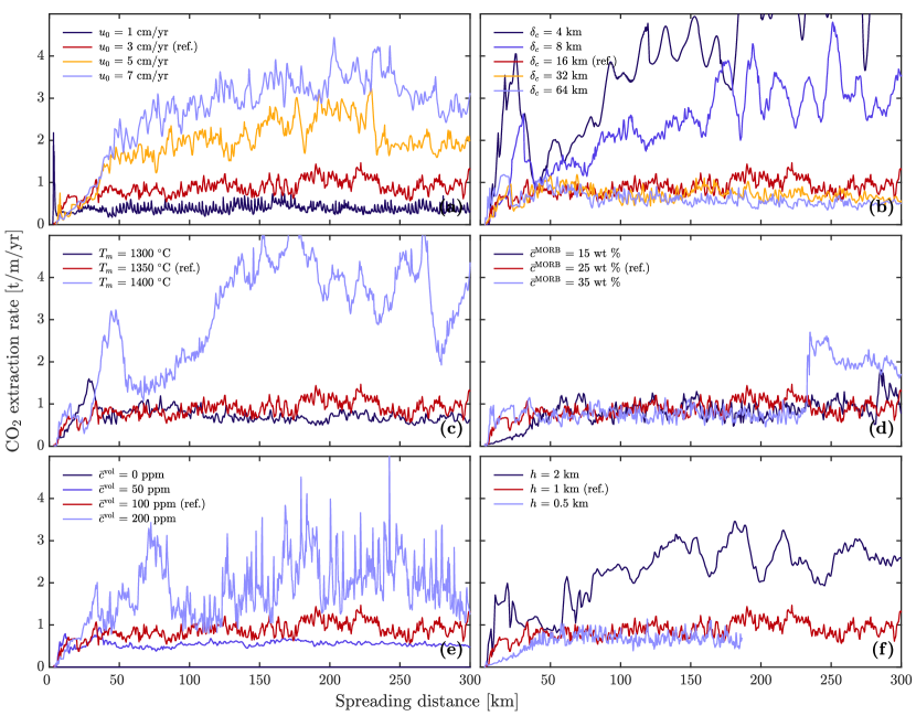
Figure S6: Time series of CO₂ extraction rate for all parameter choices. Results plotted against spreading distance. Time averages extracted over interval from 180–300 km. The resolution tests in h show that CO₂ extraction in the reference case is well resolved at reference conditions.

References

- Aharonov et al. (1995) Aharonov, E., Whitehead, J.A., Kelemen, P.B., Spiegelman, M., 1995. Channeling instability of upwelling melt in the mantle. J Geophys Res 100, 20433–20450. doi:10.1029/95JB01307.
- Asimow et al. (2004) Asimow, P.D., Dixon, J.E., Langmuir, C.H., 2004. A hydrous melting and fractionation model for mid‐ocean ridge basalts: Application to the Mid‐Atlantic Ridge near the Azores. Geochem Geophys Geosyst 5. doi:10.1029/2003GC000568.
- Asimow and Langmuir (2003) Asimow, P.D., Langmuir, C.H., 2003. The importance of water to oceanic mantle melting regimes. Nature 421, 815–820. doi:10.1038/nature01429.
- Balay et al. (2010) Balay, S., Brown, J., Buschelman, K., Eijkhout, V., Gropp, W.D., Kaushik, D., Knepley, M.G., McInnes, L.C., Smith, B.F., Zhang, H., 2010. PETSc Users Manual. Technical Report ANL-95/11 - Revision 3.4. Argonne National Laboratory.
- Balay et al. (2011) Balay, S., Brown, J., Buschelman, K., Gropp, W.D., Kaushik, D., Knepley, M.G., McInnes, L.C., Smith, B.F., Zhang, H., 2011. PETSc Web page. URL: http://www.mcs.anl.gov/petsc.
- Braun et al. (2000) Braun, M., Hirth, G., Parmentier, E.M., 2000. The effects of deep damp melting on mantle flow and melt generation beneath mid-ocean ridges. Earth Planet Sci Lett 176, 339–356. doi:10.1016/S0012-821X(00)00015-7.
- Burley and Katz (2015) Burley, J.M.A., Katz, R.F., 2015. Variations in mid-ocean ridge CO2 emissions driven by glacial cycles. Earth Planet Sci Lett 426, 246–258. doi:10.1016/j.epsl.2015.06.031.
- Cartigny et al. (2008) Cartigny, P., Pineau, F., Aubaud, C., Javoy, M., 2008. Towards a consistent mantle carbon flux estimate: Insights from volatile systematics (H 2 O/Ce, D, CO 2/Nb) in the North Atlantic mantle (14 N and 34 N). Earth Planet Sci Lett 265, 672–685. doi:10.1016/j.epsl.2007.11.011.
- Crisp (1984) Crisp, J.A., 1984. Rates of magma emplacement and volcanic output. J Volcan Geotherm Res 20, 177–211. doi:10.1016/0377-0273(84)90039-8.
- Crowley et al. (2015) Crowley, J.W., Katz, R.F., Huybers, P.J., Langmuir, C.H., Park, S.H., 2015. Glacial cycles drive variations in the production of oceanic crust. Science 347, 1237–1240. doi:10.1126/science.1261508.
- Dalton et al. (2014) Dalton, C.A., Langmuir, C.H., Gale, A., 2014. Geophysical and geochemical evidence for deep temperature variations beneath mid-ocean ridges. Science 344, 80–83. doi:10.1126/science.1249466.
- Dasgupta and Hirschmann (2006) Dasgupta, R., Hirschmann, M.M., 2006. Melting in the Earth’s deep upper mantle caused by carbon dioxide. Nature 440, 659–662. doi:10.1038/nature04612.
- Dasgupta and Hirschmann (2010) Dasgupta, R., Hirschmann, M.M., 2010. The deep carbon cycle and melting in Earth’s interior. Earth Planet Sci Lett 298, 1–13. doi:10.1016/j.epsl.2010.06.039.
- Dasgupta et al. (2013) Dasgupta, R., Mallik, A., Tsuno, K., Withers, A.C., Hirth, G., Hirschmann, M.M., 2013. Carbon-dioxide-rich silicate melt in the Earth’s upper mantle. Nature 493, 211–215. doi:10.1038/nature11731.
- Elliott and Spiegelman (2003) Elliott, T., Spiegelman, M., 2003. Melt migration in oceanic crustal production: a U-series perspective, in: R.L. Rudnick, H.H., Turekian, K. (Eds.), The Crust. Elsevier-Pergamon. volume 3 of Treatise on Geochemistry, pp. 465–510.
- Gale et al. (2014) Gale, A., Langmuir, C.H., Dalton, C.A., 2014. The global systematics of ocean ridge basalts and their origin. J Petrol 55, 1051–1082. doi:10.1093/petrology/egu017.
- Galer and O’Nions (1986) Galer, S.J.G., O’Nions, R.K., 1986. Magmagenesis and the mapping of chemical and isotopic variations in the mantle. Chem Geol 56, 45–61. doi:10.1016/0009-2541(86)90109-9.
- Havlin et al. (2013) Havlin, C., Parmentier, E.M., Hirth, G., 2013. Dike propagation driven by melt accumulation at the lithosphere–asthenosphere boundary. Earth Planet Sci Lett 376, 20–28. doi:10.1016/j.epsl.2013.06.010.
- Hebert and Montési (2010) Hebert, L.B., Montési, L.G.J., 2010. Generation of permeability barriers during melt extraction at mid-ocean ridges. Geochem Geophys Geosyst 11, Q12008. doi:10.1029/2010GC003270.
- Hirano (2011) Hirano, N., 2011. Petit-spot volcanism: A new type of volcanic zone discovered near a trench. Geochem J 45, 157–167. doi:10.2343/geochemj.1.0111.
- Hirschmann et al. (1999) Hirschmann, M.M., Asimow, P.D., Ghiorso, M.S., Stolper, E.M., 1999. Calculation of peridotite partial melting from thermodynamic models of minerals and melts. III. Controls on isobaric melt production and the effect of water on melt production. J Petrol 40, 831–851. doi:10.1093/petroj/40.5.831.
- Hirth and Kohlstedt (2003) Hirth, G., Kohlstedt, D., 2003. Rheology of the upper mantle and the mantle wedge: A view from the experimentalists, in: Eiler, J. (Ed.), Inside the Subduction Factory. Am Geophys Union. volume 138 of Geophysical Monograph, pp. 83–105.
- Hirth and Kohlstedt (1996) Hirth, G., Kohlstedt, D.L., 1996. Water in the oceanic upper mantle: implications for rheology, melt extraction and the evolution of the lithosphere. Earth Planet Sci Lett 144, 93–108. doi:10.1016/0012-821X(96)00154-9.
- Huybers and Langmuir (2009) Huybers, P., Langmuir, C., 2009. Feedback between deglaciation, volcanism, and atmospheric CO2. Earth Planet Sci Lett 286, 479–491. doi:10.1016/j.epsl.2009.07.014.
- Huybers and Langmuir (2017) Huybers, P., Langmuir, C.H., 2017. Delayed CO2 emissions from mid-ocean ridge volcanism as a possible cause of late-Pleistocene glacial cycles. Earth Planet Sci Lett 457, 238–249. doi:10.1016/j.epsl.2016.09.021.
- Katz (2008) Katz, R., 2008. Magma dynamics with the enthalpy method: Benchmark solutions and magmatic focusing at mid-ocean ridges. J Petrol 49, 2099–2121. doi:10.1093/petrology/egn058.
- Katz (2010) Katz, R., 2010. Porosity-driven convection and asymmetry beneath mid-ocean ridges. Geochem Geophys Geosyst 10. doi:10.1029/2010GC003282.
- Katz et al. (2007) Katz, R., Knepley, M., Smith, B., Spiegelman, M., Coon, E., 2007. Numerical simulation of geodynamic processes with the Portable Extensible Toolkit for Scientific Computation. Phys Earth Planet Inter 163, 52–68. doi:10.1016/j.pepi.2007.04.016.
- Kawakatsu et al. (2009) Kawakatsu, H., Kumar, P., Takei, Y., Shinohara, M., Kanazawa, T., Araki, E., Suyehiro, K., 2009. Seismic Evidence for Sharp Lithosphere-Asthenosphere Boundaries of Oceanic Plates. Science 324, 499–502. doi:10.1126/science.1169499.
- Kelemen and Manning (2015) Kelemen, P.B., Manning, C.E., 2015. Reevaluating carbon fluxes in subduction zones, what goes down, mostly comes up. Proc Natl Acad Sci doi:10.1073/pnas.1507889112.
- Kelemen et al. (1995) Kelemen, P.B., Shimizu, N., Salters, V.J.M., 1995. Extraction of mid-ocean-ridge basalt from the upwelling mantle by focused flow of melt in dunite channels. Nature 375, 747–753. doi:10.1038/375747a0.
- Keller and Katz (2015) Keller, T., Katz, R.F., 2015. R_DMC Online repository. URL: https://bitbucket.org/tokeller/r_dmc.
- Keller and Katz (2016) Keller, T., Katz, R.F., 2016. The role of volatiles in reactive melt transport in the asthenosphere. J Petrol 57, 1073–1108. doi:10.1093/petrology/egw030.
- Klein and Langmuir (1987) Klein, E.M., Langmuir, C.H., 1987. Global correlations of ocean ridge basalt chemistry with axial depth and crustal thickness. J Geophys Res 92, 8089–8115. doi:10.1029/JB092iB08p08089.
- Kono et al. (2014) Kono, Y., Kenney-Benson, C., Hummer, D., Ohfuji, H., Park, C., Shen, G., Wang, Y., Kavner, A., Manning, C.E., 2014. Ultralow viscosity of carbonate melts at high pressures. Nature Commun 5, 5091. doi:10.1038/ncomms6091.
- Lachenbruch (1976) Lachenbruch, A., 1976. Dynamics of a passive spreading center. J Geophys Res 81, 1883–1902. doi:10.1029/JB081i011p01883.
- Langmuir et al. (1992) Langmuir, C., Klein, E., Plank, T., 1992. Petrological systematics of mid-oceanic ridge basalts: constraints on melt generation beneath ocean ridges, in: Phipps Morgan, J., Blackman, D., Sinton, J. (Eds.), Mantle flow and melt generation at mid-ocean ridges. Am Geophys Union. volume 71 of Geophysical Monograph, pp. 183–280.
- Le Voyer et al. (2017) Le Voyer, M., Kelley, K.A., Cottrell, E., Hauri, E.H., 2017. Heterogeneity in mantle carbon content from CO2-undersaturated basalts. Nature Commun 8, 14062. doi:10.1038/ncomms14062.
- McKenzie (1984) McKenzie, D., 1984. The generation and compaction of partially molten rock. J Petrol 25, 713–765. doi:10.1093/petrology/25.3.713.
- McKenzie (2000) McKenzie, D., 2000. Constraints on melt generation and transport from U-series activity ratios. Chem Geol 162, 81–94. doi:10.1016/S0009-2541(99)00126-6.
- McKenzie and Bickle (1988) McKenzie, D., Bickle, M.J., 1988. The volume and composition of melt generated by extension of the lithosphere. J Petrol 29, 625–679. doi:10.1093/petrology/29.3.625.
- Mei et al. (2002) Mei, S., Bai, W., Hiraga, T., Kohlstedt, D.L., 2002. Influence of melt on the creep behavior of olivine–basalt aggregates under hydrous conditions. Earth Planet Sci Lett 201, 491–507. doi:10.1016/S0012-821X(02)00745-8.
- Mian and Tozer (1990) Mian, Z.U., Tozer, D.C., 1990. No water, no plate tectonics: convective heat transfer and the planetary surfaces of Venus and Earth. Terra Nova 2, 455–459. doi:10.1111/j.1365-3121.1990.tb00102.x.
- Michael and Graham (2015) Michael, P.J., Graham, D.W., 2015. The behavior and concentration of CO2 in the suboceanic mantle: Inferences from undegassed ocean ridge and ocean island basalts. Lithosphere 236-237, 338–351. doi:10.1016/j.lithos.2015.08.020.
- Montési et al. (2011) Montési, L.G.J., Behn, M.D., Hebert, L.B., Lin, J., Barry, J.L., 2011. Controls on melt migration and extraction at the ultraslow Southwest Indian Ridge 10∘–16∘E. J Geophys Res–Solid Earth 116. doi:10.1029/2011JB008259.
- Müntener et al. (2001) Müntener, O., Kelemen, P.B., Grove, T.L., 2001. The role of H 2 O during crystallization of primitive arc magmas under uppermost mantle conditions and genesis of igneous pyroxenites: an experimental study. Contrib mineral Petrol 141, 643–658. doi:10.1007/s004100100266.
- O’Hara (1985) O’Hara, M.J., 1985. Importance of the ‘shape’ of the melting regime during partial melting of the mantle. Nature 314, 58–62. doi:10.1038/314058a0.
- Olugboji et al. (2016) Olugboji, T.M., Park, J., Karato, S.I., Shinohara, M., 2016. Nature of the seismic lithosphere-asthenosphere boundary within normal oceanic mantle from high-resolution receiver functions. Geochem Geophys Geosyst doi:10.1002/2015GC006214.
- Pilet et al. (2011) Pilet, S., Baker, M.B., Müntener, O., Stolper, E.M., 2011. Monte Carlo Simulations of Metasomatic Enrichment in the Lithosphere and Implications for the Source of Alkaline Basalts. J Petrol 52, 1415–1442. doi:10.1093/petrology/egr007.