Next-to-Leading Order Corrections to Higgs Boson Pair Production in Gluon Fusion

Abstract:

We present a calculation of the next-to-leading order QCD corrections to the production of Higgs boson pairs in gluon fusion keeping the full dependence on the mass of the top quark. The virtual corrections, involving two-loop integrals with up to four mass scales, have been calculated numerically and we present an efficient algorithm to obtain accurate results of the virtual amplitude using numerical integrations. Taking the top quark mass into account we obtain significant differences compared to results obtained in the heavy top limit.

1 Introduction

Studying the production of Higgs boson pairs at the LHC is important to scrutinize the mechanism of electroweak symmetry breaking, because this process involves self-interactions of three Higgs bosons and a measurement of this coupling can be directly related to the potential of the Higgs field.

The dominant production mechanism for Higgs boson pairs at the LHC is gluon fusion mediated by a top-quark loop. The cross section of this process has first been calculated at leading order (LO) in Ref. [1, 2]. Approximated next-to-leading order (NLO) results have been obtained in Ref. [3] using the Born-improved Higgs Effective Field Theory (HEFT). In this approximation the NLO corrections are calculated in the heavy top limit, supplemented with a re-scaling by a factor of $B(m_{t})/B(m_{t}\rightarrow\infty)$, where B is the LO result. Using this approximation also NNLO [4, 5, 6] and resummed [7, 8] results have been calculated recently.

In contrast to single Higgs production, it is expected that the heavy top-quark approximation gives only a poor description of Higgs boson pair production since this process peaks in phase space regions where the top-quark mass is not the largest energy scale. Therefore, different methods to improve on the HEFT result emerged during the last few years. In Refs. [9, 10] the $m_{t}\rightarrow\infty$ limit has only been used to calculate the virtual corrections, whereas the full dependence on $m_{t}$ has been kept in the real radiation contribution. Another approach has been applied in Refs. [11, 12, 13], where an expansion in $1/m_{t}^{2}$ has been used to improve the prediction for the cross section. In Ref. [12], see also the presentation in Ref. [14], this expansion has also been used to improve the predictions for the NNLO contributions. These two methods for improvements on the HEFT result indicated that the top-quark mass effects should give a contribution of $\mathcal{O}(10\%)$ at NLO.

In this talk we present the NLO corrections obtained in Ref. [15], where the full dependence on the top-quark mass has been kept throughout the calculation. The two-loop integrals appearing in the virtual corrections have been calculated numerically using an interface to the program SecDec [16].

This calculation is a first step towards the construction of an automated tool for the calculation of general multi-loop amplitudes, based on the programs GoSam [17, 18] and SecDec. The progress on these developments along with details on the tools used for the calculation have been presented in the talk of S. Jones [19]. In the following, we therefore give only a brief overview of these tools and we focus on details of the numerical evaluation of the virtual amplitude and on the phenomenological results.

2 Calculation

Figure 1: Representative Feynman diagrams for the LO, virtual, and real emission contributions.

2.1 Computational Setup

Representative Feynman diagrams contributing Higgs boson pair production in gluon fusion are shown in Fig. 1. The amplitude of the underlying $2\rightarrow 2$ process

$$g(p_{1})+g(p_{2})\rightarrow h(p_{3})+h(p_{4})$$ (1)

can be decomposed into two form factors $F_{1},\,F_{2}$ as

$${\cal M}_{ab}=\delta_{ab}\epsilon_{1}^{\mu}\epsilon_{2}^{\nu}\,{\cal M}_{\mu\nu},\quad {\cal M}^{\mu\nu}=F_{1}(s,t,m_{h}^{2},m_{t}^{2},d)\;T_{1}^{\mu\nu}+F_{2}(s,t,m_{h}^{2},m_{t}^{2},d)\;T_{2}^{\mu\nu}\;,$$ (2)

where $\epsilon_{1}^{\mu},\,\epsilon_{2}^{\nu}$ are the polarization vectors of the gluons with color indices $a,\,b$, and with the Mandelstam variables $s=(p_{1}+p_{2})^{2}$, $t=(p_{3}-p_{1})^{2}$ and $u=(p_{3}-p_{2})^{2}$. The two tensor structures are

$$T_{1}^{\mu\nu}=g^{\mu\nu}-\frac{p_{1}^{\nu}\,p_{2}^{\mu}}{p_{1}\cdot p_{2}}\;,$$ (3)

$$T_{2}^{\mu\nu}=g^{\mu\nu}+\frac{m_{h}^{2}\,p_{1}^{\nu}\,p_{2}^{\mu}-2\,(p_{1}\cdot p_{3})\,p_{3}^{\nu}\,p_{2}^{\mu}-2\,(p_{2}\cdot p_{3})\,p_{3}^{\mu}\,p_{1}^{\nu}+2\,(p_{1}\cdot p_{2})\,p_{3}^{\nu}\,p_{3}^{\mu}}{p_{T}^{2}\,(p_{1}\cdot p_{2})}$$ (4)

with $p_{T}^{2}=(tu-m_{h}^{4})/s$. To calculate the virtual amplitude, we constructed a multi-loop extension of the program GoSam which, after generating the Feynman diagrams using Qgraf [20], uses Form [21, 22] to apply projectors onto the two form factors and for further processing of the expressions. To facilitate the use of reduction programs, we created an interface to Reduze [23] and matched all loop integrals to integral families, leading to expressions for $F_{1}$ and $F_{2}$ containing $\sim$10.000 integrals with up to 7 propagators and 4 inverse propagators. These expressions have been validated by comparing them to a second implementation entirely based on Qgraf and Reduze.

The reduction of the integrals to master integrals turned out to be very challenging and we therefore fixed the numeric values $m_{t}=173\,\mathrm{GeV}$ and $m_{h}=125\,\mathrm{GeV}$ during reduction, thus reducing the number of appearing mass scales by one. With this simplification, the reduction to masters has been obtained for all the planar integrals, but we didn’t achieve a full reduction for the non-planar 6 and 7 propagator integrals using the programs Reduze [23], Fire [24] or LiteRed [25]. For simplifying the numerical evaluation of these integrals, we therefore rewrote the inverse propagators in terms of scalar products, leading to non-planar 7 propagator integrals of up to rank 4.

After the partial reduction, the expressions for the amplitude contained 145 planar master integrals as well as 70 mostly unreduced non-planar tensor integrals, leading to a total of 327 integrals when including integrals that differ by a crossing. We calculated these integrals using the program SecDec, which decomposes the integrals into sectors leading to finite Feynman parameter integrals at each order in $\epsilon=(4-d)/2$, where $d$ is the dimension of space-time. We modified SecDec such that the integrands of latter integrals are written to a library, which allows us to call them directly from our code for the amplitude evaluation and we dynamically adjust the number of sampling points as discussed in the next section. For the numerical integration we use a quasi-Monte Carlo algorithm based on a rank-one lattice rule [26, 27], which for sufficiently smooth integrands obeys a scaling $\Delta\propto n^{-1}$ of the integration error with the number of sampling points.

The real emission contribution involves up to one-loop pentagon diagrams with a top-quark appearing in the loop. The corresponding amplitudes have been generated using the program GoSam and we used the dipole subtraction algorithm [28] to deal with the infrared singularities.

2.2 Numerical Evaluation of the Virtual Amplitude

After form factor decomposition and partial reduction, the virtual amplitude $\mathcal{M}_{V}$ is determined by the two form factors $F_{1}$ and $F_{2}$, which are a linear combination of 327 two-loop integrals $I_{j}$,

$$F_{i}(s,t,m_{t}^{2},m_{t}^{2},\epsilon)=\sum_{j}f_{i,j}(s,t,m_{t}^{2},m_{t}^{2},\epsilon)\cdot I_{j}(s,t,m_{t}^{2},m_{t}^{2},\epsilon),$$ (5)

with multi-variate rational functions $f_{i,j}$ as coefficients. For the numeric calculation of the integrals, it is convenient to factor out an arbitrary mass scale $M$ as well as a prefactor $c_{j}(\epsilon)$ containing the $\Gamma$-functions arising from Feynman parametrization and integration of the loop momenta. This leads to

$$I_{j}(s,t,m_{t}^{2},m_{t}^{2};\epsilon)=\left(\frac{\mu^{2}}{M^{2}}\right)^{2\epsilon}c_{j}(\epsilon)\,M^{m_{j}}\,\hat{I}_{j}\left(\frac{s}{M^{2}},\frac{t}{M^{2}},\frac{m_{t}^{2}}{M^{2}},\frac{m_{t}^{2}}{M^{2}};\epsilon\right),$$ (6)

where $\mu$ is the mass scale of dimensional regularization and the exponent $m_{j}$ is given by the mass dimension of integral $I_{j}$. After applying sector decomposition using SecDec, each loop integral $\hat{I}_{j}$ is decomposed into multiple sectors $s$, which can be expanded in $\epsilon$, leading to a Laurent series

$$\hat{I}_{j}\left(\frac{s}{M^{2}},\frac{t}{M^{2}},\frac{m_{t}^{2}}{M^{2}},\frac{m_{t}^{2}}{M^{2}};\epsilon\right)=\sum_{s}\,\sum_{e>e_{s}^{\mathrm{min}}}\,\epsilon^{e}\,\hat{I}_{j,s,e}\left(\frac{s}{M^{2}},\frac{t}{M^{2}},\frac{m_{t}^{2}}{M^{2}},\frac{m_{t}^{2}}{M^{2}}\right),$$ (7)

and the integrals $\hat{I}_{j,s,e}$ can be integrated numerically over the Feynman parameter space. Rearranging the terms of Eqs. (5)-(7), we can write the two form factors as

$$F_{i}(\epsilon)=\left(\frac{\mu^{2}}{M^{2}}\right)^{2\epsilon}\cdot\underbrace{\sum_{j,s,e}\hat{I}_{j,s,e}\cdot a_{i,j,e}(\epsilon)}_{A_{i}}$$ (8)

and expand the coefficients

$$a_{i,j,e}(\epsilon)=\epsilon^{e}M^{m_{j}}c_{j}(\epsilon)f_{i,j}(\epsilon)$$ (9)

up to $\mathcal{O}(\epsilon^{0})$, where the dependence of the form factor, integral and coefficients on $s,t,m_{t}^{2}$ and $m_{t}^{2}$ has been suppressed. This form allows us to obtain the results of the two form factors (including their poles in $\epsilon$), while computing each integral only once. Furthermore, applying a similar procedure to the calculation of the LO amplitude and mass counter terms, Eq. (8) allows us to vary the renormalization scale $\mu_{R}$ without recomputing $A_{i}$.

Sector decomposition allows us to write the amplitude in terms of finite integrals which we can calculate numerically, however, it also leads to a significant increase in the number of integrals. After decomposition and expansion in $\epsilon$, the 327 integrals $I_{j}$ are replaced by $\sim$11.000 integrals $\hat{I}_{j,s,e}$. With this large number of integrals, it is not advisable to evaluate each integral with a pre-defined accuracy or number of sampling points. Assuming that each integral gave the same contribution to the amplitude, each integral would be required with a precision of $\mathcal{O}(10^{-4})$ to obtain an amplitude result with an accuracy of 1%. However, cancellations between various integrals can spoil the accuracy of the amplitude result and a significant increase in the precision for these integrals might be required. On the other hand, one wants to avoid calculating integrals to very high accuracy if they only give a small contribution.

We therefore dynamically set the number of sampling points for each integral depending on its contribution to the error estimate of the amplitude result and depending on the time required for each integrand evaluation. For simplicity, we now consider the evaluation of only one form factor at a given power in $\epsilon$ and we write Eq. (8) as $F=\sum_{j}(a_{j}\,I_{j})$. To efficiently calculate $F$ to a given accuracy $\varepsilon_{\mathrm{rel}}=\Delta_{F}/F$, we set the number of sampling points for each integral by minimizing the total time

$$T=\sum_{j}t_{j}+\lambda\left(\Delta_{F}^{2}-\sum_{j}a_{j}^{2}\Delta_{j}^{2}\right),$$ (10)

where $t_{j}$ and $\Delta_{j}$ are the integration time and absolute error of integral $I_{j}$, and $\lambda$ is a Lagrange multiplier ensuring the accuracy constraint. After an initial run of each integral with a fixed number of sampling points, we set the number of sampling points according to Eq. (10) assuming that the error of the individual integrals $I_{j}$ scales as $\Delta_{j}\propto t_{j}^{-e}$. While we obtain a scaling with $e=1$ for most of the integrals, some of the integrals don’t fulfill the smoothness condition of the quasi-Monte Carlo method leading to worse convergence of these integrals and we therefore set $e=0.7$ globally in the program.

3 Phenomenological Results

We present results for the cross section of Higgs boson pair production at the LHC with a center of mass energy of $\sqrt{s}=14\,\mathrm{TeV}$. The masses of the Higgs boson and top quark are set to $m_{h}=125$ GeV and $m_{t}=173$ GeV, and we use the PDF4LHC15_nlo_100_pdfas [29, 30, 31, 32] parton distribution functions, along with the corresponding value for $\alpha_{s}$. The central value of the renormalization and factorization scale are set to $\mu_{R}=\mu_{F}=m_{HH}/2$ and we estimate the scale uncertainty by simultaneously varying these scales by a factor of 2.

We obtain a total cross section of

$$\sigma^{NLO}=32.90^{+14\%}_{-13\%}\,\mathrm{fb}\pm 0.3\%\,(\mathrm{stat.})\pm 0.1\%\,(\mathrm{int.}).$$

where we state the statistical error stemming from the number of evaluated phase points and the additional error due to the numerical integration of the virtual amplitude in addition to the scale uncertainty. This result is a factor of $\sim$1.6 larger than the LO result $\sigma^{LO}=19.85^{+28\%}_{-21\%}$ and 14% smaller than the result $\sigma^{\mathrm{NLO}}_{\mathrm{HEFT}}=38.32^{+18\%}_{-15\%}$ obtained in the Born-improved HEFT approximation.

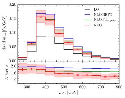
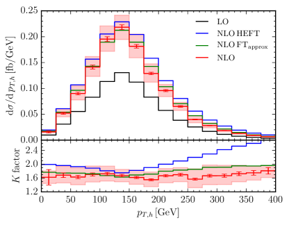
Figure 2: Differential distributions of the invariant mass $m_{hh}$ of the Higgs boson pair and transverse momentum $p_{T,h}$ of the Higgs bosons. The center of mass energy is set to $\sqrt{s}=14$ TeV and the bands result from scale variations by a factor of two around the central scale $\mu=m_{hh}/2$. We compare our predictions to the approximated NLO results using the Born-improved HEFT and taking the top-quark mass effects into account only in the real emission contributions, FT_approx.

The differential dependence of the cross section on the invariant mass $m_{hh}$ of the Higgs bosons as well as the dependence on their transverse momentum $p_{T,h}$ is shown in Fig. 2. We find good agreement of our predictions with the approximated NLO results for invariant masses below 400$\,\mathrm{GeV}$, where the HEFT is expected to be valid. However, for large invariant masses we observe that taking the top-quark mass effects into account reduces the cross section by about 20-30% compared to the HEFT result. In the $p_{T,h}$-distribution we obtain a nearly constant K factor, whereas the HEFT approximation leads to a significant increase of the NLO corrections for high transverse momenta. Compared to the HEFT results, the NLO FT_approx results, which include the top-quark mass effects in the real emission, lead to better agreement with the full NLO result. However, also this approximation fails to describe the decreasing K factor for high invariant masses.

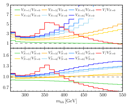
Figure 3: Comparison of the virtual contributions $V$ with the results obtained by an expansion in $1/m_{t}^{2}$. Results are shown at the amplitude level with the definitions of $V_{N}$ and $V^{\prime}_{N}$ given in Eq. (11).

Fig. 3 shows a comparison of the virtual amplitude with an expansion in $1/m_{t}^{2}$ obtained from private communication with the authors of Ref. [12]. We combine the renormalized amplitude with the $\mathbf{I}$-operator defined in Ref. [28] and define

$$V_{N}=d\sigma^{\mathrm{virt}}_{N}+d\sigma^{\mathrm{LO}}_{N}\otimes\mathbf{I}\quad\mathrm{and}\quad V^{\prime}_{N}=V_{N}\cdot\frac{d\sigma^{\mathrm{LO}}}{d\sigma^{\mathrm{LO}}_{N}}$$ (11)

where $d\sigma^{LO}_{N}$ and $d\sigma^{V}_{N}$ are the LO and virtual contribution expanded up to order $1/m_{t}^{2N}$. The figure shows that the expansion converges to the full virtual amplitude in the region well below the top-quark threshold at $m_{hh}=2m_{t}$ but we obtain large differences at higher invariant masses.

4 Conclusions

We presented a computation of the NLO corrections to Higgs boson pair production in gluon fusion, keeping the full dependence on the top-quark mass throughout the calculation. Since the results for the two-loop integrals appearing in the virtual amplitude are not known analytically, we calculate these numerically and we have shown how an accurate result for the amplitude can be obtained using this numerical approach. Using the methods presented here, we plan to develop a program for the automated generation and evaluation of multi-loop amplitudes.

Our predictions show that the effects of the top-quark mass are important and they have to be taken into account to obtain reliable predictions for Higgs boson pair production in gluon fusion. For low invariant masses of the di-Higgs system we find good agreement of the HEFT result with our predictions. However, we observe that the inclusion of the top-quark mass reduces the cross section by $\sim$30% in phase space regions where $m_{hh}$ or $p_{T,h}$ is large. For the total cross section at 14$\,\mathrm{TeV}$ we obtain a reduction of 14% compared to the result obtained the Born-improved HEFT approximation.

- [1] E. W. N. Glover and J. J. van der Bij, Higgs Boson Pair Production via Gluon Fusion, Nucl. Phys. B309 (1988) 282.
- [2] T. Plehn, M. Spira, and P. M. Zerwas, Pair production of neutral Higgs particles in gluon-gluon collisions, Nucl. Phys. B479 (1996) 46–64, [hep-ph/9603205]. [Erratum: Nucl. Phys.B531,655(1998)].
- [3] S. Dawson, S. Dittmaier, and M. Spira, Neutral Higgs boson pair production at hadron colliders: QCD corrections, Phys. Rev. D58 (1998) 115012, [hep-ph/9805244].
- [4] D. de Florian and J. Mazzitelli, Two-loop virtual corrections to Higgs pair production, Phys. Lett. B724 (2013) 306–309, [arXiv:1305.5206].
- [5] D. de Florian and J. Mazzitelli, Higgs Boson Pair Production at Next-to-Next-to-Leading Order in QCD, Phys. Rev. Lett. 111 (2013) 201801, [arXiv:1309.6594].
- [6] J. Grigo, K. Melnikov, and M. Steinhauser, Virtual corrections to Higgs boson pair production in the large top quark mass limit, Nucl. Phys. B888 (2014) 17–29, [arXiv:1408.2422].
- [7] D. Y. Shao, C. S. Li, H. T. Li, and J. Wang, Threshold resummation effects in Higgs boson pair production at the LHC, JHEP 07 (2013) 169, [arXiv:1301.1245].
- [8] D. de Florian and J. Mazzitelli, Higgs pair production at next-to-next-to-leading logarithmic accuracy at the LHC, JHEP 09 (2015) 053, [arXiv:1505.07122].
- [9] R. Frederix, S. Frixione, V. Hirschi, F. Maltoni, O. Mattelaer, P. Torrielli, E. Vryonidou, and M. Zaro, Higgs pair production at the LHC with NLO and parton-shower effects, Phys. Lett. B732 (2014) 142–149, [arXiv:1401.7340].
- [10] F. Maltoni, E. Vryonidou, and M. Zaro, Top-quark mass effects in double and triple Higgs production in gluon-gluon fusion at NLO, JHEP 11 (2014) 079, [arXiv:1408.6542].
- [11] J. Grigo, J. Hoff, K. Melnikov, and M. Steinhauser, On the Higgs boson pair production at the LHC, Nucl. Phys. B875 (2013) 1–17, [arXiv:1305.7340].
- [12] J. Grigo, J. Hoff, and M. Steinhauser, Higgs boson pair production: top quark mass effects at NLO and NNLO, Nucl. Phys. B900 (2015) 412, [arXiv:1508.00909].
- [13] G. Degrassi, P. P. Giardino, and R. Groeber, On the two-loop virtual QCD corrections to Higgs boson pair production in the Standard Model, arXiv:1603.00385.
- [14] J. Hoff, Top quark mass effects in Higgs boson pair production up to NNLO, PoS LL2016 (2016) 024, [arXiv:1606.05847].
- [15] S. Borowka, N. Greiner, G. Heinrich, S. P. Jones, M. Kerner, J. Schlenk, U. Schubert, and T. Zirke, Higgs Boson Pair Production in Gluon Fusion at Next-to-Leading Order with Full Top-Quark Mass Dependence, Phys. Rev. Lett. 117 (2016), no. 1 012001, [arXiv:1604.06447]. [Erratum: Phys. Rev. Lett. 117, 079901 (2016)].
- [16] S. Borowka, G. Heinrich, S. P. Jones, M. Kerner, J. Schlenk, and T. Zirke, SecDec-3.0: numerical evaluation of multi-scale integrals beyond one loop, Comput. Phys. Commun. 196 (2015) 470–491, [arXiv:1502.06595].
- [17] G. Cullen, N. Greiner, G. Heinrich, G. Luisoni, P. Mastrolia, et al., Automated One-Loop Calculations with GoSam, Eur.Phys.J. C72 (2012) 1889, [arXiv:1111.2034].
- [18] G. Cullen et al., GS-2.0: a tool for automated one-loop calculations within the Standard Model and beyond, Eur. Phys. J. C74 (2014), no. 8 3001, [arXiv:1404.7096].
- [19] S. P. Jones, Automation of 2-loop amplitude calculations, PoS LL2016 (2016) 069.
- [20] P. Nogueira, Automatic Feynman graph generation, J.Comput.Phys. 105 (1993) 279–289.
- [21] J. Vermaseren, New features of FORM, math-ph/0010025.
- [22] J. Kuipers, T. Ueda, J. Vermaseren, and J. Vollinga, FORM version 4.0, Comput.Phys.Commun. 184 (2013) 1453–1467, [arXiv:1203.6543].
- [23] A. von Manteuffel and C. Studerus, Reduze 2 - Distributed Feynman Integral Reduction, arXiv:1201.4330.
- [24] A. V. Smirnov, FIRE5: a C++ implementation of Feynman Integral REduction, Comput. Phys. Commun. 189 (2014) 182–191, [arXiv:1408.2372].
- [25] R. N. Lee, LiteRed 1.4: a powerful tool for reduction of multiloop integrals, J. Phys. Conf. Ser. 523 (2014) 012059, [arXiv:1310.1145].
- [26] J. Dick, F. Y. Kuo, and I. H. Sloan, High-dimensional integration: The quasi-monte carlo way, Acta Numerica 22 (2013) 133–288.
- [27] Z. Li, J. Wang, Q.-S. Yan, and X. Zhao, Efficient Numerical Evaluation of Feynman Integral, Chinese Physics C 40, No. 3 (2016) 033103, [arXiv:1508.02512].
- [28] S. Catani and M. H. Seymour, A General algorithm for calculating jet cross-sections in NLO QCD, Nucl. Phys. B485 (1997) 291–419, [hep-ph/9605323]. [Erratum: Nucl. Phys.B510,503(1998)].
- [29] J. Butterworth et al., PDF4LHC recommendations for LHC Run II, arXiv:1510.03865.
- [30] S. Dulat, T.-J. Hou, J. Gao, M. Guzzi, J. Huston, P. Nadolsky, J. Pumplin, C. Schmidt, D. Stump, and C. P. Yuan, New parton distribution functions from a global analysis of quantum chromodynamics, Phys. Rev. D93 (2016), no. 3 033006, [arXiv:1506.07443].
- [31] L. A. Harland-Lang, A. D. Martin, P. Motylinski, and R. S. Thorne, Parton distributions in the LHC era: MMHT 2014 PDFs, Eur. Phys. J. C75 (2015), no. 5 204, [arXiv:1412.3989].
- [32] NNPDF Collaboration, R. D. Ball et al., Parton distributions for the LHC Run II, JHEP 04 (2015) 040, [arXiv:1410.8849].