A geometrical look at MOSPA Estimation using Transportation Theory

Abstract

It was shown in [6] that the Wasserstein distance is equivalent to the Mean Optimal Sub-Pattern Assignment (MOSPA) measure for empirical probability density functions. A more recent paper [7], extends on it by drawing new connections between the MOSPA concept, which is getting a foothold in the multi-target tracking community, and the Wasserstein distance, a metric widely used in theoretical statistics. However, the comparison between the two concepts has been overlooked. In this letter we prove that the equivalence of Wasserstein distance with the MOSPA measure holds for general types of probability density function. This non trivial result allows us to leverage one recent finding in the computational geometry literature to show that the Minimum MOPSA (MMOSPA) estimates are the centroids of additive weighted Voronoi regions with a specific choice of the weights.

I Introduction

The mean squared error (MSE) has long been the dominant quantitative performance metric in the field of signal processing. An estimator which minimizes the MSE is referred to as a minimum MSE (MMSE) estimator. In target tracking [9], the traditional problem is posed as the finding of the MMSE estimate of the target states. Since the MMSE estimate is given by the expected value of the posterior probability density function, which intrinsically has an ordering (labeling) of the states, the MMSE estimator can be classified as a labeled estimator. In some applications the labeling of the objects is not relevant. For these problems, it is more reasonable to instead of minimizing the MSE try to minimize a measure which eschews target labeling. A measure that has received an increasing amount of attention in the later years, and which can be seen as a natural extension of the MSE to label-free estimation, is the OSPA metric [10]. The OSPA is a label-free correspondent to the squared error. The MOSPA, which is the counterpart of the MSE, was introduced in [11] where the authors also described how to calculate the MMOSPA estimates. Explicit solutions for MMOSPA estimation are only available in the scalar case [12]. In [13] and references therein, various techniques for approximating MMOSPA estimates are presented . In [7], a connection between the empirical MMOSPA estimate and the Wasserstein barycenter for point cloud was established. This result builds upon the Lemma 1 in [7] which states that the Wasserstein distance coincides with the MOSPA for empirical probability densities defined on sets with the same cardinality. The Wasserstein distance defined using empirical probability densities can be computed solving a linear programming (LP) problem [6, 14]. The LP formulation of the transportation problem, is also known as the Hitchcock-Koopmans transportation problem [15]. The results of this letter are twofold:

• We extend the result in [7, 6] for a wider class of probability measures, to draw a theoretical connection between the MOSPA measure and the more general transportation problem, known as Monge-Kantorovich transportation problem [2, 4, 5].

• This main finding, in conjunction with a recent result in computational geometry [16], allows us to provide new insights on MOSPA estimation revealing interesting geometrical structure and properties of the MMOSPA estimates.

The remainder of the paper is organized as follows. In Section II we formalize our problem. Section III contains our main theoretical contributions and also provides a geometrical interpretation of the MMOSPA and in Section IV we summarize our conclusions.

II Problem Formulation

In this section, we will present the main problem of this letter. We will first define notations used in this paper and then we will define notions of interest such as OSPA, MOSPA, MMOSPA and the Wasserstein distance.

Let us assume that there are $N$ objects of interest, which reside in the space $\mathbb{R}^{n_{x}}$ with $n_{x}$ being a positive integer. The states of all the objects are denoted by the sequence of vectors $\{\mathbf{X}_{i}\}_{i=1}^{N}\in\mathbb{R}^{n_{x}}$. The vectors $\{\mathbf{X}_{i}\}_{i=1}^{N}$ are stochastic with a joint probability measure $\mu$ defined on $\mathbb{R}^{N\times n_{x}}$. Moreover we assume that $\mu$ is absolutely continuous with respect to the Lebesque measure [1].

Define the stacked vector $\mathbf{X}$ as follows :

$$\mathbf{X}=\left[\mathbf{X}_{1}^{T}\quad\mathbf{X}_{2}^{T}\quad\ldots\quad\mathbf{X}_{N}^{T}\right]^{T}$$ (1)

For a sequence of vectors of states estimates $\{\mathbf{\hat{X}}_{i}\}_{i=1}^{N}$, let us define the stacked vector of states estimates $\mathbf{\hat{X}}$ as in equation (1).

Define $\Pi_{N}$ to be the set of permutations on the set $\{1,2,\ldots,N\}$. For a permutation $\pi\in\Pi_{N}$ and a stacked vector defined in equation (1), let us define $\pi(\mathbf{X})$ as follows:

$$\pi(\mathbf{X})=\left[\mathbf{X}_{\pi(1)}^{T}\quad\mathbf{X}_{\pi(2)}^{T}\quad\ldots\quad\mathbf{X}_{\pi(N)}^{T}\right]^{T}$$ (2)

The vector $\pi(\mathbf{X})$ permutes the single objects states in $\mathbf{X}$ according to $\pi$. Define OSPA [8] as follows :

$$d^{OSPA}(\mathbf{X},\mathbf{\hat{X}})=\min_{\pi\in\Pi_{N}}\sum_{i=1}^{N}\left(\mathbf{X}_{i}-\mathbf{\hat{X}}_{\pi(i)}\right)^{T}\left(\mathbf{X}_{i}-\mathbf{\hat{X}}_{\pi(i)}\right)$$ (3)

Let us define OSPA using the stacked notation as follows:

$$d^{OSPA}(\mathbf{X},\mathbf{\hat{X}})=\min_{\pi\in\Pi_{N}}\left(\mathbf{X}-\pi\left(\mathbf{\hat{X}}\right)\right)^{T}\left(\mathbf{X}-\pi\left(\mathbf{\hat{X}}\right)\right)$$ (4)

Let us define MOSPA and the relative MMOSPA as follows [11] :

$$MOSPA\left(\mu,\mathbf{\hat{X}}\right)=E_{\mu}\left[d^{OSPA}(\mathbf{X},\mathbf{\hat{X}})\right]$$ (5)

$$\mathbf{\hat{X}}^{MMOSPA}=\textrm{arg}\min_{\mathbf{\hat{X}}}E_{\mu}\left[d^{OSPA}(\mathbf{X},\mathbf{\hat{X}})\right]$$ (6)

Let us define the $p^{\textrm{th}}$ Wasserstein distance [2], [3] between two probability measures on some space $M$ as:

$$W_{p}(\nu_{1},\nu_{2}):=\left(\inf_{\gamma\in\Gamma(\nu_{1},\nu_{2})}\int_{M\times M}d(x,y)^{p}\,\mathrm{d}\gamma(x,y)\right)^{1/p}$$ (7)

$\Gamma(\nu_{1},\nu_{2})$ denotes the set of all joint measures on $M\times M$ with marginal measures $\nu_{1}$ and $\nu_{2}$. For this paper we use the Euclidean distance for $d$, $p=2$ and $M$ is the space $\mathbb{R}^{N\times n_{x}}$.

We are now ready to formulate the main problem of this letter. It will be shown that the following equation holds, which connects the MOSPA and the Wasserstein distance:

$$MOSPA\left(\mu,\mathbf{\hat{X}}\right)=W^{2}_{2}(\mu,\nu)$$ (8)

where $\nu$ is a discrete measure which depends on $\mathbf{\hat{X}}$ and it will be defined later.

Let us define the collection of sets $\mathbb{S}_{\pi}\left(\mathbf{\hat{X}}\right)$ for all $\pi\in\Pi_{N}$ as follows:

$$\begin{split}\mathbb{S}_{\pi}\left(\mathbf{\hat{X}}\right)=\{\mathbf{X}\in\mathbb{R}^{N\times n_{x}}:\left(\mathbf{X}-\pi\left(\mathbf{\hat{X}}\right)\right)^{T}\left(\mathbf{X}-\pi\left(\mathbf{\hat{X}}\right)\right)\\ \leq\left(\mathbf{X}-\tilde{\pi}\left(\mathbf{\hat{X}}\right)\right)^{T}\left(\mathbf{X}-\tilde{\pi}\left(\mathbf{\hat{X}}\right)\right),\forall\tilde{\pi}\in\Pi_{N}\}\end{split}$$ (9)

It follows then, that for any two different permutations $\pi$ and $\tilde{\pi}$, the set $\mathbb{S}_{\pi}\cap\mathbb{S}_{\tilde{\pi}}$ has Lebesque measure zero, hence its measure with respect to $\mu$ is also zero. Here we assume without loss of generality that $\mathbf{\hat{X}}_{i}\neq\mathbf{\hat{X}}_{j},\forall i\neq j$.

For a fixed deterministic $\mathbf{\hat{X}}$, let us define the discrete random variable (d.r.v.) $\mathbf{Y}$ as follows :

$$\mathbf{Y}=\sum_{\pi\in\Pi_{N}}\pi\left(\mathbf{\hat{X}}\right)\cdot\mathbb{I}_{\mathbb{S}_{\pi}}\left(\mathbf{X}\right)$$ (10)

From equation (10) we conclude that $\mathbf{Y}$ takes value $\pi\left(\mathbf{\hat{X}}\right)$ with probability $\mu(\mathbb{S}_{\pi})$ for all $\pi\in\Pi_{N}$. Then, the d.r.v. $\mathbf{Y}$ induces the discrete probability measure $\nu$ on $\mathbb{R}^{N\times n_{x}}$ which is defined as follows:

$$\nu(x)=\sum_{\pi\in\Pi_{N}}\mu(\mathbb{S}_{\pi})\cdot\delta\left(x-\pi\left(\mathbf{\hat{X}}\right)\right)$$ (11)

The measure $\nu$, which depends on $\mathbf{\hat{X}}$, will play the role of measure $\nu$ from equation (8).

III Main Results

In this section, we will present the main results of this letter. We will formulate and prove Theorem 1, which shows the connection between the Wasserstein distance and the MOSPA for general measures and then we will prove certain geometrical properties of the optimal MOSPA.

III-A MOSPA meets Wasserstein in the general case

In this subsection, we will formulate and prove the main theorem of the paper, in which we establish the connection between the Wasserstein distance and the MOSPA.

Theorem 1.

Given a probability measure $\mu$ defined on $\mathbb{R}^{N\times n_{x}}$, a vector $\hat{X}\in\mathbb{R}^{N\times n_{x}}$ and a probability measure $\nu$ defined in equation (11), the following holds:

$$E_{\mu}\left[d^{OSPA}(\mathbf{X},\mathbf{\hat{X}})\right]=W^{2}_{2}(\mu,\nu)$$ (12)

Proof.

We first show that

$$E_{\mu}\left[\left(\mathbf{X}-\mathbf{Y}\right)^{T}\left(\mathbf{X}-\mathbf{Y}\right)\right]=E_{\mu}\left[d^{OSPA}(\mathbf{X},\mathbf{\hat{X}})\right]$$ (13)

with $\mathbf{Y}$ defined in equation (10).

$$\begin{split}E_{\mu}&\left[\left(\mathbf{X}-\mathbf{Y}\right)^{T}\left(\mathbf{X}-\mathbf{Y}\right)\right]\\ &=\int_{\mathbb{R}^{N\times n_{x}}}\left(\mathbf{X}-\mathbf{Y}\right)^{T}\left(\mathbf{X}-\mathbf{Y}\right)d\mu\\ &=\sum_{\pi\in\Pi_{N}}\int_{\mathbb{S}_{\pi}}\left(\mathbf{X}-\mathbf{Y}\right)^{T}\left(\mathbf{X}-\mathbf{Y}\right)d\mu\\ &\stackrel{{\scriptstyle a}}{{=}}\sum_{\pi\in\Pi_{N}}\int_{\mathbb{S}_{\pi}}\left(\mathbf{X}-\sum_{\pi\in\Pi_{N}}\pi\left(\mathbf{\hat{X}}\right)\cdot\mathbb{I}_{\mathbb{S}_{\pi}}\left(\mathbf{X}\right)\right)^{T}\\ &\quad\quad\quad\quad\quad\left(\mathbf{X}-\sum_{\pi\in\Pi_{N}}\pi\left(\mathbf{\hat{X}}\right)\cdot\mathbb{I}_{\mathbb{S}_{\pi}}\left(\mathbf{X}\right)\right)d\mu\\ &\stackrel{{\scriptstyle b}}{{=}}\sum_{\pi\in\Pi_{N}}\int_{\mathbb{S}_{\pi}}\left(\mathbf{X}-\pi\left(\mathbf{\hat{X}}\right)\right)^{T}\left(\mathbf{X}-\pi\left(\mathbf{\hat{X}}\right)\right)d\mu\\ &\stackrel{{\scriptstyle c}}{{=}}E_{\mu}\left[d^{OSPA}(\mathbf{X},\mathbf{\hat{X}})\right]\end{split}$$

The equalities ($a$) and ($b$) follow from the definition of $\mathbf{Y}$ in equation (10) and the equality ($c$) follows from the definition of $\mathbb{S}_{\pi}$ in equation (9) and the definition of OSPA in equation (4). Next we show that

$$W^{2}_{2}(\mu,\nu)\leq E_{\mu}\left[\left(\mathbf{X}-\mathbf{Y}\right)^{T}\left(\mathbf{X}-\mathbf{Y}\right)\right]$$ (14)

Equation  (10) defines the probability measure $\nu$ and moreover defines a joint measure $\gamma\in\Gamma(\mu,\nu)$. Hence, from the definition of the Wasserstein distance in equation (7), equation  (14) immediately follows. We show the reverse inequality next that

$$W^{2}_{2}(\mu,\nu)\geq E_{\mu}\left[\left(\mathbf{X}-\mathbf{Y}\right)^{T}\left(\mathbf{X}-\mathbf{Y}\right)\right]$$ (15)

Choose an arbitrary joint probability measure $\gamma\in\Gamma(\mu,\nu)$. From $\gamma$ we can define the conditional probability measure $\gamma_{\nu|\mu}$ with respect to the measure $\mu$. It follows then, that $\gamma_{\nu|\mu}$ is a discrete probability measure with the same support as $\nu$. We can write the following:

$$\begin{split}&E_{\gamma}\left[\left(\mathbf{X}-\mathbf{Y}\right)^{T}\left(\mathbf{X}-\mathbf{Y}\right)\right]\\ &=\int_{\mathbb{R}^{N\times n_{x}}\times\mathbb{R}^{N\times n_{x}}}\left(\mathbf{X}-\mathbf{Y}\right)^{T}\left(\mathbf{X}-\mathbf{Y}\right)d\gamma\\ &=\int_{\mathbb{R}^{N\times n_{x}}}\int_{\mathbb{R}^{N\times n_{x}}}\left(\mathbf{X}-\mathbf{Y}\right)^{T}\left(\mathbf{X}-\mathbf{Y}\right)d\gamma_{\nu|\mu}d\mu\\ &=\sum_{\pi\in\Pi_{N}}\int_{\mathbb{S}_{\pi}}\int_{\mathbb{R}^{N\times n_{x}}}\left(\mathbf{X}-\mathbf{Y}\right)^{T}\left(\mathbf{X}-\mathbf{Y}\right)d\gamma_{\nu|\mu}d\mu\\ &\stackrel{{\scriptstyle a}}{{\geq}}\sum_{\pi\in\Pi_{N}}\int_{\mathbb{S}_{\pi}}\int_{\mathbb{R}^{N\times n_{x}}}\left(\mathbf{X}-\pi\left(\mathbf{\hat{X}}\right)\right)^{T}\left(\mathbf{X}-\pi\left(\mathbf{\hat{X}}\right)\right)d\gamma_{\nu|\mu}d\mu\\ &\stackrel{{\scriptstyle b}}{{=}}\sum_{\pi\in\Pi_{N}}\int_{\mathbb{S}_{\pi}}\left(\mathbf{X}-\pi\left(\mathbf{\hat{X}}\right)\right)^{T}\left(\mathbf{X}-\pi\left(\mathbf{\hat{X}}\right)\right)\int_{\mathbb{R}^{N\times n_{x}}}d\gamma_{\nu|\mu}d\mu\\ &=\sum_{\pi\in\Pi_{N}}\int_{\mathbb{S}_{\pi}}\left(\mathbf{X}-\pi\left(\mathbf{\hat{X}}\right)\right)^{T}\left(\mathbf{X}-\pi\left(\mathbf{\hat{X}}\right)\right)d\mu\\ &\stackrel{{\scriptstyle c}}{{=}}E_{\mu}\left[d^{OSPA}(\mathbf{X},\mathbf{\hat{X}})\right]\end{split}$$ (16)

The inequality ($a$) follows from the definition of $\mathbb{S}_{\pi}$ in equation (9), equality ($b$) follows from the fact that $\pi\left(\mathbf{\hat{X}}\right)$ is a deterministic vector for $\mathbf{X}\in\mathbb{S}_{\pi}$, which does not depend on the conditional probability measure $\gamma_{\nu|\mu}$. The equality ($c$) follows from the definition of $\mathbb{S}_{\pi}$ in equation (9) and the definition of OSPA in equation (4). From equation (16), we conclude that

$$E_{\gamma}\left[\left(\mathbf{X}-\mathbf{Y}\right)^{T}\left(\mathbf{X}-\mathbf{Y}\right)\right]\geq E_{\mu}\left[d^{OSPA}(\mathbf{X},\mathbf{\hat{X}})\right]$$ (17)

Taking the infimum over all $\gamma\in\Gamma(\mu,\nu)$, equation (15) follows. Hence, from equation (14) and equation (15), equation  (12) follows. ∎

III-B Geometry of the optimal MMOSPA

In this subsection, we will prove that the geometry of the optimal partition from Theorem 1 satisfies certain geometric properties. It was shown in Theorem (1), that:

$$E_{\mu}\left[d^{OSPA}(\mathbf{X},\mathbf{\hat{X}})\right]=W^{2}_{2}(\mu,\nu)$$ (18)

with the measure $\nu$ being a discrete probability measure, which takes values $\pi\left(\mathbf{\hat{X}}\right)$ with probability $\mu\left(\mathcal{S}_{\pi}\right)$. Theorem 2 from [16] shows that, the optimal partition of the space $\mathcal{R}^{N\times n_{x}}$ which achieves $W^{2}_{2}(\mu,\nu)$ exists, it is unique and it is given by the additive weighted Voronoi regions defined as follows:

$$\begin{split}\mathcal{C}_{i}\left(\mathcal{P},\Omega\right)=\{\mathbf{X}\in\mathcal{R}^{N\times n_{x}}:&\left(\mathbf{X}-p_{i}\right)^{T}\left(\mathbf{X}-p_{i}\right)+\omega_{i}\leq\\ &\left(\mathbf{X}-p_{j}\right)^{T}\left(\mathbf{X}-p_{j}\right)+\omega_{j},\\ &\forall j\in\{1,2,\ldots,N!\}\}\end{split}$$ (19)

where $\mathcal{P}=\{p_{1},\ldots,p_{N!}\}\subseteq\mathcal{R}^{N\times n_{x}}$ is a set of centroids and $\Omega=\{\omega_{1},\ldots,\omega_{N!}\}\subseteq\mathcal{R}$ is a set of real numbers.

Proposition 1.

$\pi\left(\mathbf{\hat{X}}\right)$ are the centroids of the additive weighted Voronoi regions $\mathcal{C}_{i}\left(\mathcal{P},\Omega\right)$, with $\omega_{i}=\omega_{j},\forall i\neq j$.

Proof.

For a given $\mathbf{\hat{X}}$, it follows from Theorem 2 in [16], that $\mathcal{C}_{i}\left(\mathcal{P},\Omega\right)$ are optimal sets. Moreover from the proof of Theorem 1, it follows that the sets $\mathcal{S}_{\pi}$ are optimal. Then it can be seen that the sets $\mathcal{S}_{\pi}$ are the same as the sets $\mathcal{C}_{i}\left(\mathcal{P},\Omega\right)$ with $\omega_{i}=\omega_{j},\forall i\neq j$. ∎

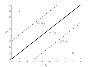
Figure 1: Voronoi diagrams for the two targets case. The circles represent the two unlabeled target state estimates.

Interestingly, the results above are a dual of the results from [11] with respect to the labeling of the target states versus target states estimates. In [11], the MMOSPA estimates were fixed while $\mu$ was folded. In this letter, the measure $\mu$ remains fixed while the MMOSPA estimates define the probability measure $\nu$, which depends on the permutations of the MMOSPA estimates themselves and on the Voronoi diagrams from Proposition 1.

Figure 1 shows an example of the Voronoi diagram for MMOSPA estimates. In this case $N=2$ and $n_{x}=1$, i.e. there are two one-dimensional targets. Moreover, let the sequence of target state estimates be the set $\{-4,3\}$. Then, for a realization of the vector $\mathbf{X}$ above the solid line in Figure 1, the target states estimates are represented by the vector $\left[-4\quad 3\right]$, while for a realization of the vector $\mathbf{X}$ below the solid line, the target states estimates are represented by the vector $\left[3\quad-4\right]$. The dotted lines show examples of additive Voronoi diagrams with different weights. For the case with three one-dimensional targets, there will be six different possible target approximations and six regions separated by hyperplanes in the three dimensional Euclidean space.

Remark 1.

The results in [16] and in general in transportation theory [2] hold for general distances than Euclidean and the geometrical properties from Proposition 1 remain still valid.

For example, in the case of a more general distance GOSPA (General OSPA):

$$d^{GOSPA}\left(\mathbf{X},\mathbf{\hat{X}}\right)=\left(\mathbf{X}-\pi\left(\mathbf{\hat{X}}\right)\right)^{T}\mathbf{Q}\left(\mathbf{X}-\pi\left(\mathbf{\hat{X}}\right)\right)$$ (20)

where $\mathbf{Q}$ is a positive definite matrix, the additively weigthed Voronoi diagrams are no longer symmetric (i.e. $\omega_{i}\neq\omega_{j})$. Lastly, if more general distances are used [16], the Voronoi diagrams will be separated by more general manifolds than hyperplanes [2].

IV Conclusion

The main result of this letter establishes the equivalence between the MOSPA measure, which is a concept widely used in target tracking community, and Wasserstein distance between one continuous measure and one discrete measure. This finding allowed us to draw a connection with a recent result in computational geometry [16], which showed that additively weigthed Voronoi diagrams can optimally solve some cases of the Monge-Kantorovich transportation problem, with one measure being discrete. More specifically, we were able to show that MMOSPA estimates are exactly equal to the centroid of these Voronoi diagrams for a particular choice of the weights. Revealing geometrical structures for the MMOSPA estimates advances our understanding of the MOSPA estimation problem drawing upon different scientific fields. In the future we are planning to extend the current results, if possible, to the more general case of MOSPA measure defined for sets with different cardinalities.

References

- [1] P. Billingsley, Probability and Measure, 4th ed. Wiley, 2012.
- [2] C. Villani, Optimal Transport: Old and New (Grundlehren der mathematischen Wissenschaften), 2009 ed. Springer, 2009.
- [3] L. Ambrosio, Lecture Notes on Optimal Transport Problems, Mathematical Aspects of Evolving Interfaces, Springer Verlag, Berlin, Lecture Notes in Mathematics (1812), 1–52, 2003.
- [4] L. Kantorovich, On a problem of Monge (In Russian), Uspekhi Math. Nauk. 3 (1948): pp 225-226. [English translation: J. Math. Sci.,133, 4 (2006), pp.1383.]
- [5] G. Monge, Memoire sur la theorie des deblais et de remblais, Histoire de l’Academie Royale des Sciences de Paris, avec les Memoires de Mathematique et de Physique pour la meme annee, (1781).
- [6] J. R. Hoffman and R. P. Mahler, “Multitarget miss distance via optimal assignment,” IEEE Transactions on Systems, Man, and Cybernetics-Part A: Systems and Humans, vol. 34, no. 3, pp. 327–336, 2004.
- [7] M. Baum, K. Peter, D. Uwe Hanebeck, “On wasserstein barycenters and mmospa estimation,” IEEE Signal Processing Letters, vol. 22, no. 10, pp. 1511–1515, 2015.
- [8] M. Baum, K. Peter, D. Uwe Hanebeck, “Polynomial-time algorithms for the exact MMOSPA estimate of a multi-object probability density represented by particles,” IEEE Transactions on Signal Processing, vol. 63, no. 10, pp. 2476–2484, 2015.
- [9] Y. Bar-Shalom, P. K. Willett, and X. Tian, “Tracking and data fusion,” 2011.
- [10] D. Schuhmacher, B.-T. Vo, and B.-N. Vo, “A consistent metric for performance evaluation of multi-object filters,” IEEE Transactions on Signal Processing, vol. 56, no. 8, pp. 3447–3457, 2008.
- [11] M. Guerriero, L. Svensson, D. Svensson, and P. Willett, “Shooting two birds with two bullets: how to find minimum mean ospa estimates,” in Information Fusion (FUSION), 2010 13th Conference on. IEEE, 2010, pp. 1–8.
- [12] D. Crouse, P. Willett, Y. Bar-Shalom, L. Svensson, “Aspects of mmospa estimation,” in Proceedings of the 50th IEEE Conference on Decision and Control, CDC-ECC 2011, Orlando, FL, 12-15 December 2011, pp. 6001–6006.
- [13] D. F. Crouse, “Advances in displaying uncertain estimates of multiple targets,” in Proceedings of SPIE - The International Society for Optical Engineering, 23 May 2013, pp. 874504-874504-31.
- [14] Y. Rubner, C. Tomasi, and L. J. Guibas, “The earth mover’s distance as a metric for image retrieval,” International journal of computer vision, vol. 40, no. 2, pp. 99–121, 2000.
- [15] S. Rao, Engineering Optimization: Theory and Practice: Fourth Edition. John Wiley and Sons, 6 2009.
- [16] D. Geiß, R. Klein, and R. Penninger, “Optimally Solving a Transportation Problem Using Voronoi Diagrams,” in Computing and Combinatorics, vol. 7434 of the series Lecture Notes in Computer Science, Springer, 2012, pp 264-274.