Quantitative measure for the spin-charge separation in two dimensional Hubbard model

Abstract

We introduce a quantitative measure of spin-charge separation, $\zeta(t)$ which is based on the difference between the fluctuations with respect to background of the spin and charge profiles at any time $t$ and is suitable for studying the non-equilibrium dynamics of excitations in strongly correlated systems. This quantity is not only a direct measure of the spin-charge separation in strongly correlated systems, but its long time behaviour can further serve as a possible order parameter for the interaction induced (Mott) insulating state. Within the numerically exact diagonzalization we calculate this quantity for the two dimensional Hubbard model away from Half filling. Our quantitative measure in chain, ladder and two-dimensional geometries gives the same order of magnitude for the quantity of spin-charge separation. Furthermore from the temporal behaviour of $\zeta(t)$ a threshold time can be identified that provides clues onto the breakdown of underlying Mott insulating phase.

I Introduction

Spin and charge are part of the identity of an electron as a fundamental particle in vacuum. But in condensed matter where a bunch of electrons come together, if the spatial dimension is restricted to one dimension (1D), these two quantum characteristics of electrons tend to behave as if they are distinct entities which is referred to as the spin-charge separation (SCS). In one dimensional conductors the spin and charge move with two different velocities that is determined by Coulomb interaction strength Tomonaga ; Luttinger ; Voit . This makes the interacting electron liquids in 1D quite different from those in three-dimensional Fermi liquids. While the excitations of three dimensional Fermi liquids are electron and hole-like quasiparticles, in the excitation spectrum of 1D liquids known as Tomonaga-Luttinger liquids there are no such quasiparticles, but instead there are collective modes that carry spin-only or charge-only Giamarchi . This remarkable phenomenon has been experimentally observed in 1D GaAs/AlGaAs heterostructures where spin and charge modes with different velocities were identified West . Characteristics of tunneling into 1D spin-charge separated systems are also observed Schofield . Also signatures of spin-charge separation have been observed in variety of systems including carbon nano-tubes McEuen . The photoemission spectra of Au chains on Si(111) surface show power-laws predicted by Tomonaga-Luttinger theory Baer ; Nagaosa . Electromagnetic response of class of organic salts Schwartz is also consistent with the picture of spin-charge separation. For insulating 1D materials where charge degrees of freedom are localized by strong Coulomb interactions, the spin degrees of freedom retain their kinetic energy and can roam about. Angular resolved photoemission data in 1D copper-oxide chain material SrCuO₂ backed by exact diagonalization calculations of 1D t-J model support the picture of spin and charge separation in 1D insulators Kim as well. This separation gives rise to large optical nonlinearity in such Mott insulators Tohyama . Theoretical understanding of the separation of spin and charge in Mott insulators is based on the work of Ogata and Shiba OgataShiba who used the exact Bethe ansatz solution of Lieb and Wu LiebWu to prove exactly that the ground state of the 1D Hubbard model in the limit of very large Coulomb repulsion factorizes into a Slater determinants of spin-less fermions and a bosonic wave function (even with respect to particle exchange) that is the ground state of a related spin chain Hamiltonian. Implications of spin-charge separation in the dielectric response of a 1D Mott insulator compound Sr₂CuO₃ were also experimentally investigated Uchida .

Therefore the low-energy part of the spectrum of excitations in 1D systems are exhausted by collective modes of charge and spin. In 1D conductors the charge mode is gapless, while in the 1D insulators the charge mode is gapped by strong Coulomb interactions. While the quasi particle excitations in three dimensional Fermi liquids are electron and hole-like, and in 1D are collective spin and charge modes, understanding the nature of excitations in two-dimensional (2D) interacting systems remains an unsettled quest. Many unusual properties of strongly correlated two-dimensional cuprate superconductors are ascribed to some form of non-Fermi liquid behaviour Anderson2DLuttinger . Anderson emphasizes that the spin-charge separation is the key to understanding the physics of high temperature cuprates AndersonPhysC . Standard approaches to non-Fermi liquid states are based on auxiliary particle methods RMPslave which build on the assumption of separate particles carrying spin and charge of the physical electron. Dynamics of a single-hole in a frustrated 2D quantum magnet supports the picture of spin-charge separation Poilblanc . Quantum Monte Carlo study of the t-J model also supports the SCS in 2D TKLee . Furthermore cluster perturbation theory study of spectral properties of 1D and 2D Hubbard model also supports the SCS in two-dimensional Hubbard model Senechal .

Since in 2D there is no exact solution akin to Leib-Wu solution of the 1D Hubbard model, although other methods based on quantum Monte carlo may also be applicable Hanke ; simone , the unbiased method of choice to study the exact dynamics of excitations in 2D system is the numerically exact diagonalization JafariED and related technique of density matrix renormalization group white ; rmpdmrg . This approach was already taken by Jagla, Hallberg, and Balseiro in 1993 Balseiro . Using very small clusters affordable in 1993, and with qualitative pictures they concluded that spin and charge do separate in 1D, while in 2D there is no sign of spin-charge separation. The 1D aspect of this work was revisited by Kollath and coworkers using time-dependent density-matrix renormalization group to study the real time dynamics of the Hubbard model in a 1D chain who confirmed the spin-charge separation beyond the low-energy theory of Tomonaga-Luttinger liquid Kollath . They applied the model to describe cold Fermi gases in a harmonic trap.

In this work we revisit this problem and introduce a direct and quantitative measure for the separation of spin and charge degrees of freedom. Our time-dependent quantity, $\zeta(t)$, is defined as the difference in the profiles of spin and charge density averaged over the entire space satisfies the following properties: (1) It is zero at $t=0$ when a test particle is added to the ground state of the system, and increases with time when we have spin-charge separation. (2) For $U=0$ limit of the Hubbard model where the ground state is a Slater determinant it remains zero at all later times $t$. (3) The $\lim_{t\to\infty}\zeta(t)$ is zero for conducting phase, and non-zero for Mott insulating phase, and therefore $\zeta(\infty)$ can serve as an Mott insulating order parameter obtained from non-equilibrium dynamics. Therefore this quantity contains information about the nature of charge localization in the Mott phase. Equipped with this quantity, we undertake exact diagonalization investigation of one and two-dimensional Hubbard model and we find quite surprisingly that within our measure, the order of magnitude of the spin-charge separation quantity in 2D is the same as the one in 1D. Our non-equilibrium study of the excitation dynamics further shows that in the Mott insulating phase, the charge carriers are localized in long time-scales, while in the short time-scales the charge density fluctuates spatially. The cross-over between these two regimes can provides clues to the breakdown of Mott insulating phase.

II Model and method

We consider the Hubbard model given by

$$\hat{H}=-\sum_{\langle i,j\rangle,\sigma}\hat{c}^{\dagger}_{i\sigma}\hat{c}_{j\sigma}++U\sum^{L}_{i=1}\hat{n}_{i\uparrow}\hat{n}_{i\downarrow},$$ (1)

where $c^{\dagger}_{i\sigma}$ creates an electron at site $i$ with spin $\sigma$, the hopping amplitude has been set as the unit for the energy, the Hubbard $U$ is the on-site interaction strength, $\hat{n}_{i\sigma}=c^{\dagger}_{i\sigma}c_{i\sigma}$ is the fermion occupation number and $L$ is the number of lattice sites. The site label $i$ can refer to any lattice.

In this work we will consider the real-time evolution of an electron added to the ground state of the above Hubbard model in 1D, ladder and 2D square lattice and various fillings. The lattice constant in this work are assumed to be the unit of length. In our simulation we start with the ground state of a system with $N=N_{\uparrow}+N_{\downarrow}$ electrons and then add a new electron at momentum $\langle k_{x}\rangle=\pi/2$. After adding the new electron the total number of electrons becomes $N+1$ which defines the filling fraction as $n=(N+1)/L$.

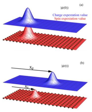
Figure 1: (Color online) Schematic representation of separation of charge (blue) and spin (red). (a) At initial time $t=0$ spin and charge are concentrated around the same region. (b) After the wave function has evolved by a large $U$ Hubbard Hamiltonian, the spin and charge densities are piled in different regions of space and propagate with different velocities. Quantities $X_{Q}$ and $X_{S}$ are ”center of mass” of the charge and spin as defined in Eq. (5).

In the two-dimensional case $k_{y}=0$, meaning that the initial wave-packet has no spatial dispersion along the $y$ direction. We calculate the ground state wave function with the standard Lanczos algorithm. Then at time $t=0$ we add an electron in the wave-packet with a non-zero kinetic energy and denote the resulting state with $|\psi(t=0)\rangle$. The kinetic energy of the added wave-packet moves it forward. At a later time $t$ the wave function evolves to $|\psi(t)\rangle$ according to standard quantum evolution formula Thijssen ,

$$|\psi(t+dt)\rangle\approx\left[1-i\hat{H}dt-\hat{H}^{2}(dt)^{2}/2\right]|\psi(t)\rangle,$$ (2)

where we have set $\hbar=1$. At every step of time-evolution we normalize the wave function to ensure the stable propagation up to longer times. We have explicitly cross-checked the results of above evolution algorithm against the brute force dynamics,

$$|\psi(t)\rangle=\sum_{n}e^{-iE_{n}t}|\psi(t=0)\rangle,$$ (3)

for small few-particle Hilbert spaces where all excited states energies $E_{n}$ are numerically accessible by exact diagonalization of the Hamiltonian matrix. Typical values of $dt$ in our natural units (where $\hbar$ and hopping amplitude are set to unity) are $10^{-4}$. We have furthermore checked that the quantum evolution given by Eq. (2) is stable with respect to variation in $dt$ across two orders of magnitude $dt=10^{-3}-10^{-5}$.

The spin and charge density operators $\hat{S}_{i}$ and $\hat{Q}_{i}$ at every lattice site can be defined as,

$$\hat{S}_{i}=(n_{i\uparrow}-n_{i\downarrow}),~{}~{}~{}~{}~{}~{}\hat{Q}_{i}=(n_{i\uparrow}+n_{i\downarrow}).$$ (4)

Notice that we have deliberately dropped the factor of $\dfrac{1}{2}$ in definition of spin density. This will be clear when we define our quantitative measure of the spin-charge separation. At any later time $t$ where the wave function has evolved to $|\psi(t)\rangle$, we can obtain the expectation values of the above operators to define $\langle{S}_{i}(t)\rangle=\langle\psi(t)|\hat{S}_{i}|\psi(t)\rangle$ and $\langle Q_{i}(t)\rangle=\langle\psi(t)|\hat{Q}_{i}|\psi(t)\rangle$. The spatial profile of $\langle S_{i}(t)\rangle$ and $\langle Q_{i}(t)\rangle$ as a function of space variable $i$ coincide at $t=0$. At later times the spatial profiles of charge and spin start to differ from each other when large enough Hubbard $U$ is used to generate the dynamics of an added electron. As pointed out by Jagla et al Balseiro the SCS can be qualitatively seen in 1D as the separation of the peaks of the spatial profiles of the above two functions. The system sizes considered in 1993 in Ref. Balseiro and the qualitative assessment lead them to conclude that within their exact diagonalization study they do not find spin-charge separation in 2D square lattice. In this work we consider much larger system sizes and furthermore define the quantity of spin-charge separation as follows:

The spatially averaged background for the spin and charge densities before adding the new electron is given by $S_{\rm bg}=0$ and $Q_{\rm bg}=N/L$. The spatial fluctuations defined by $\delta S_{i}=\langle S_{i}(t)\rangle-S_{\rm bg}$ and $\delta Q_{i}=\langle Q_{i}(t)\rangle-Q_{\rm bg}$ can be used to define,

$$X_{Q}(t)=\sum_{i=1}^{L}\delta Q_{i}(t)~{}x_{i},~{}~{}~{}X_{S}(t)=\sum_{i=1}^{L}\delta S_{i}(t)~{}x_{i},$$ (5)

which is spatial average of charge and spin densities and can be viewed as the worldline of the center of mass of charge and spin. The standard deviations from the above averages can also be defined to assign an ”error bar” (due to quantum effects) to each of the worldlines. The above quantities represent the charge and magnetic polarization of the medium. Now we are ready to define the quantity of spin-charge separation as,

$$\zeta^{2}(t)=\dfrac{1}{L}\sum^{L}_{i=1}(\delta{Q}_{i}-\delta{S}_{i})^{2},$$ (6)

which is nothing but the spatial average of the difference in the fluctuations of charge and spin density at every instant $t$ of time. At $t=0$ charge and spin have identical profiles therefore one always has $\zeta(t=0)=0$. Moreover at $U=0$ where the ground state of system is a simple slater determinant this quantity remains zero for all later times. We show that the quantity $\zeta(t)$ has a great deal of information not only on the separation of spin and charge, but also on the localization of charge in the Mott insulator and its associated time scales. Indeed the $\zeta(t)$ being some sort of fluctuation will contain – within the general fluctuation-dissipation theorem – information about the response of system to external perturbation: As we will discuss in this work, from the short time behaviour of $\zeta(t)$, one can infer information on the breakdown of a Mott insulating state in response to an strong applied voltage.

Therefore the function $\zeta(t)$: (i) Quantifies the spin-charge separation and hence provides a measure to compare the amount of separation in various settings, e.g. between one and two dimensions. (ii) This measure understands the difference between the Mott insulating and conducting phases. (iii) This measure has ideas about the non-equilibrium charge (and spin) dynamics and essential time (and hence energy) scales at which a Mott insulator behaves as an insulator. The later means that instead of applying a high enough voltage to study the breakdown of Mott insulator as has been previously done within the exact diagonalization method by Oka and collaborators Oka , we consider the evolution of quantity $\zeta$ with time. A Mott insulating behaviour sets in, only after a threshold time which can be associated via the uncertainity principle with a breakdown.

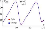
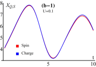
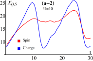
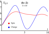
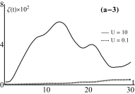
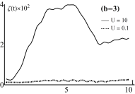
Figure 2: Worldlines of charge (blue) and spin (red), $X_{Q,S}$ defined in Eq. (5) along with the separation quantity $\zeta(t)$. (a) First column corresponds to 1D chain, and the second column (b) corresponds to a two-leg ladder. Panels (a-1) and (b-1) present the charge and spin wordlines for $U=0.1$ while (a-2) and (b-2) correspond to $U=10$. The third row represents the separation quantity for chain (a-3) and ladder (b-3) for the two values of $U=10,0.1$ as indicated in the legend. The one dimensional chain has $30$ sites and $N+1=3$ electrons and the ladder is $12\times 2$ with $N+1=5$ electrons.

III Spin and charge worldlines

In Fig. 2 we have plotted the worldlines of charge and spin as defined in Eq.(5) with blue and red lines, respectively. The left column (a) corresponds to a 1D Hubbard chain with $L=30$ sites and $N+1=3$ electrons, and the right column (b) corresponds to a $12\times 2$ two-leg ladder with $N+1=5$ electrons. Panels (a-1) and (b-1) represent the worldline of charge (blue) and spins (red) for $U=0.1$. Panels (a-2) and (b-2) present the same data for $U=10$. Panels (a-3) and (b-3) display the separation quantity $\zeta(t)$ as a function of time for the above vlaues of Hubbard $U$ as indicated in the legend. Both densities are far from half-filling. As can be seen in the first row, when the Hubbard $U=0.1$ is small, the worldlines of spin and charge in both chain and ladder geometries almost coincide. For $U=10$ in the second row the worldines of spin and charge show clear separation in both chain and ladder geometries. In both cases the charge reaches the right end before the spin. The ”returning” behaviour of the worldlines is an artifact of periodic boundary conditions for the finite sizes employed in this simulations as the charge (spin) density leaving e.g. the right end, re-enters due to periodic boundary conditions from the left side which results in effective movement of the ”center of mass” of charge (spin) to the left. In realistic situations spin and charge keep moving in the right directions and they will be asymptotically decoupled. Moreover one can see that in both chain and ladder geometries spin and charge move with different velocities, and that spin diffuses faster than charge voit93 .

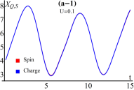
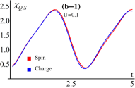
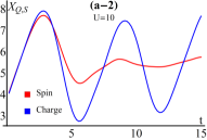
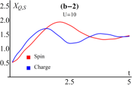
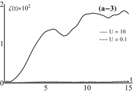
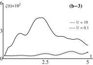
Figure 3: (Color online) Worldlines of charge (blue) and spin (red), $X_{Q,S}$ defined in Eq. (5) along with the separation quantity $\zeta(t)$. The left column (a) corresponds to $12\times 4$ lattice with $N+1=3$ electrons. The right column (b) corresponds to $4\times 4$ lattice with $N+1=7$ electrons. The blue (red) worldlines correspond to charge (spin). The first row correspons to $U=0.1$ while the second row corresponds to $U=10$. Third row represents the $\zeta(t)$ parameter for the two lattices.

Let us move to the third row of Fig. 2. Panels (a-3) and (b-3) corresponding to chain and ladder geomtries show the quantity $\zeta(t)$ as a function of time $t$ for two values of Hubbard $U$ indicated in the legend. As can be seen for $U=0.1$ this quantity is nearly zero. By increasing $U$ to $10$, this measure of spin-charge separation significantly deviates from zero. It is important to notice that the present measure of separation in chain and ladder geometry gives comparable numbers of the order of $\sim 10^{-2}$. As can be seen in both (a-3) and (b-3) cases the $U=10$ result for $\zeta$ has similar behaviours: At $t=0$ it is zero by construction. It reaches a maximum at some intermediate time scales of the order of couple of $\hbar$ (Note that the kinetic energy scale is unit of energy). Then for $t\to\infty$ it again tends to zero.

Now that we have demonstrated the how the quantity $\zeta(t)$ works in chain and ladder geometry, let us discuss how the quantity $\zeta(t)$ works in 2D geometry. Fig. 3 presents the same set of data as in Fig. 2 for two 2D square lattices. The left column (a) corresponds to $12\times 4$ lattice with $N+1=3$ electrons and the right column (b) corresponds to $4\times 4$ lattice with $N+1=7$ electrons, both of which are away from Mott phase at small values of Hubbard $U$. In both cases the charge (blue) and spin (red) worldlines are shown for $U=0.1$ (first row) and $U=10$ (second row). As can be seen qualitatively from the worldlines in both (a) and (b) lattices with different densities, the spin and charge tend to separate for strong enough correlations. There is however an important difference between panels (a-2) and (b-2) in this figure corresponding to a density of $3/48=0.0625$ and $7/16=0.4375$, respectively. If we had long range interactions, the role of interactions in low density case would be much more pronounced than the higher density limit. However, since we are dealing with the short range Hubbard interaction, the effect of Hubbard $U$ is more manifest in higher densities. That is why in panel (a-2) it takes a longer time for the spin-charge separation to show up in $\zeta(t)$, while in panel (b-2) at very initial time steps the velocities (slops of the worldlines) become different. At higher densities electric charges meet more often and the Hubbard $U$ will have more profound effect. To see this more precisely, in the third row we plot our separation parameter $\zeta(t)$. As can be seen in both figures, in the $U=10$ case this parameter turns out to be on the scale of $10^{-2}$. Therefore to the extent that spin and charge are separated in one dimension, they show very same quantitative behaviour in 2D and strong correlations causes spin and charge densities to propagate with different velocities. This also demonstrates how the quantity $\zeta(t)$ encodes the difference in the worldlines of spin and charge ”center of masses”. Note that densities considered here are quite below the half-filling and the antiferromagnetic instabilities do not concern us here.

IV Conductor versus insulator

The behavior $\lim_{t\to\infty}\zeta(t)=0$ is indeed an indicator of conducting properties: Since in the conducting phase both spin and charge diffuse and ultimately spread over the whole system giving a flat spatial distribution of spin and charge (equal to the background value), hence $\zeta(\infty)=0$ in a conducting phase. On the other hand, in a Mott insulating state, the spin keeps diffusing, while the charge ultimately freezes in space giving a $\lim_{t\to\infty}\zeta(t)\neq 0$. To this extent the long time behavior of $\zeta(t)$ – ideally the $t\to\infty$ limit, but practically a couple of $\hbar/$hopping – can serve as a possible ”order parameter” for a Mott state. Let us see how does it work in various geometreis.

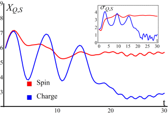
Figure 4: (Color online) The spin (red) and charge (blue) worldlines for a Mott insulator at $U=30$, on a $12\times 2$ ladder with $N+1=5$ electrons. The inset represents the the standard deviation of the charge (blue) and spin (red) density.

In Fig. 4 we plotted the worldlines of spin and charge for a $12\times 2$ ladder with $5$ electrons and $U=30$. The inset of the top panel shows the spread of the center of mass of charge and spin. The worldline of the spin shows that the spin center of mass saturates towards the center of ladder which due to periodic boundary condition means that the spin has uniformly spread all over the lattice. To see this more clearly, in the inset we have shown the standard deviation of the center of mass of charge and spin. The charge woldline on the other hand shows that the charge freezes at a different point of the lattice. At initial times steps the charge density moves along the ladder. But beyond a certain time scale the charge density starts to feel the effect of strong Hubbard $U$. This onset time is controlled by Hubbard $U$ and the density of electrons. Once the charge realizes that it lives in a Mott insulator, it freezes at some point. The inset of the top panel shows the spread of charge (blue) and spin (red) densities. As can be seen the spin has undergone a diffusion and has been delocalized all over the ladder, while the charge has been localized in some spot of the ladder. The initial three peak structures in both worldines and spread of the charge density indicate that due to periodic boundary condition the charge density has revolved three times across the ladder length.

The localization of charge and delocalization of spin density is a distinct feature of Mott insulating state which has been naturally captured in the worldlines of spin and charge densities. What our worldlines indicate further is that for the charge added to a Mott state it takes some time to ”figure out” that will live in a Mott insulating environment. Before this threshhold time, $t_{\rm tr}$ the charge density keeps moving until the charge density learns enough about the dynamics of the Mott insulating Hamiltonian after which it stops moving. By that time the spin density has already delocalized all over the lattice. This threshhold time by uncertainity principle would correspond to a threshchold energy, meaning that a Mott insulator would conduct above a certain energy scale (voltage) $V_{\rm tr}\sim\hbar/t_{\rm tr}$ that can be interpreted as the breakdown of Mott insulating phase Oka .

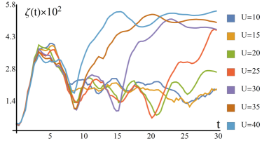
Figure 5: (Color online) The $\zeta(t)$ for $12\times 2$ ladder with a fixed $N+1=5$ electrons and variable Hubbard $U$ values indicated in the legend.

Now we are ready to demonstrate how the Mott transition shows up in our $\zeta(t)$ profiles. For this purpose in Fig. 5 we have plotted this function for the $12\times 2$ ladder with a fixed $N+1=5$ number of electrons for various values of Hubbard $U$ parameter. The early time behaviour of the $\zeta(t)$ is quite similar for all values of $U$ signalling that it is a transient behaviour. Beyond a certain time scale to the left of $t=10$ the separation quantity starts to know about the differences in Hubbard $U$. For smaller values of $U$ the $\zeta(t)$ decreases at longer times. Let us argue that this corresponds to a conducting state: The spin density already spreads and delocalizes itself irrespective of whether it is in the Mott state or conducting state. However for smaller values of $U$ corresponding to conducting state, the charge density diffuses as well, and will eventually spread uniformly over the entire ladder giving $\zeta(t\to\infty)=0$. Therefore the decreasing behaviour of $\zeta(t)$ at large $t$ is characteristic of a conducting state. In the Mott state in contrary the charge freezes at some location after a threshhold time $t_{\rm tr}$. This prevents the $\zeta$ function from diminishing. Therefore in the Mott state $\zeta$ is expected to saturate to a non-zero value. That is why for values of $U$ larger than $25$ the $\zeta$ function takes up in long times and saturates to a non-zero value.

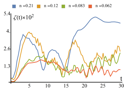
(a)

Figure 6: (Color online) Temporal profile of $\zeta(t)$ for a fixed value of $U=30$ and various values of filling fraction $n=(N+1)/L$ with $N+1=5,L=12\times 2$ $(n=0.21)$, $N+1=3,L=12\times 2$ $(n=0.12)$, $N+1=3,L=12\times 3$ $(n=0.083)$ and $N+1=3,L=12\times 4$ $(n=0.062)$.

While Fig. 5 indicates that the temporal profile of $\zeta(t)$ contains information about the charge localization in the Mott state for various values of $U$, in Fig. 6 for a fixed value of $U=30$ we present the temporal profile of $\zeta$ for different values of filling factor $n$ indicated in the figure. In this figure we have used various lattice sizes indicated in the figure. For $U=30$, only at the highest filling factor $n=0.21$ reported here we find a saturation behaviour in $\zeta(t)$ indicating a Mott insulating phase for this filling. For lower fillings, even a value of $U$ as large as $30$ is not able to give rise charge localization behaviour. For a fixed $U$ when the filling fraction is larger, the probability of two electrons to come across each other at the same site (the double occupancy) increases. Therefore at larger $n$ a given value of Hubbard $U$ does a better job at suppressing the double occupancy. That is why in this figure for lower filling fractions the $U=30$ value is not able to localize the charges and $\zeta(t)$ decreases at large $t$.

V Summary and conclusion

In this work we have introduced a quantity based on the difference in the fluctuations of the spin and charge around their center of mass whose temporal behaviour and magnitude contains information about the spin-charge separation. Within the present $\zeta(t)$ function we find that the spin and charge do separate in 2D to the extent that they do in 1D. Further we found that the long time behaviour of this function differs for conducting states and Mott insulating states. It is zero for conducting states and non-zero for Mott insulating states. It can therefore serve as an order parameter for the Mott state. Furthermore, a threshhold time scale in the behaviour of $\zeta(t)$ that separates transient non-equilibrium behaviour from the long-time equilibrated situation reveals information about the voltage at which a Mott insulating phase breaks down.

Indeed a a two-dimensional version of Luttinger lequid theory has been postulated by Anderson AndersonHall and has been used by him to explain the temperature dependence of the Hall effect in normal state of cuprate superconductors Anderson2DLuttinger . The present work on quantification of the spin-charge separation demonstrates that spin and charge excitations of the two dimensional Hubbard model are separated and therefore the ground state of the 2D Hubbard model in low-doping does not appear to be a Fermi liquid. Further research is needed to understand the properties of such a non-Fermi liquid state in two-dimension.

VI Acknowledgement

SAJ was supported by Sharif university of technology and Alexander von Humboldt foundation.

References

- (1) S. -I. Tomonaga, Prog. Theor. Phys. 5 (1950) 544.
- (2) J. M. Luttinger, J. Math. Phys. 4 (1953) 1154.
- (3) J. Voit, Rep. Prog. Phys. 58 (1995) 977.
- (4) T. Giamarchi, Quantum Physics in One Dimension Oxford Univ. Press, (2004).
- (5) O. M. Auslaender, H. Steinberg, A. Yacoby, Y. Tserkovnyak, B. I. Halperin, K. W. Baldwin, L. N. Pfeiffer, and K. W. West, Science, 308 (2005) 88.
- (6) Y. Jompol, C. J. B. Ford, J. P. Griffiths, I. Farrer, G. A. C. Jones, D. Anderson, D. A. Ritchie, T. W. Silk, and A. J. Schofield, Science, 325 (2009) 597.
- (7) P. Segovia, D. Purdie, M. Hengsberger, and Y. Baer, Nature, 402 (1999) 504.
- (8) H. Suzuura, N. Nagaosa, Phys. Rev. B 56 (1997) 3548.
- (9) A. Schwartz, M. Dressel, G. Grüner, V. Vescoli, L. Degiorgi, T. Giamarchi, Phys. Rev. B 58 (1998) 1261.
- (10) M. Bockrath, D. H. Cobden, J. Lu, A. G. Rinzler, R. E. Smalley, L. Balents, P. L. McEuen, Naturr, 397 (1998) 598.
- (11) C. Kim, A. Y. Matsuura, Z.-X. Shen, N. Motoyama, H. Eisaki, S. Uchida, T. Tohyama, and S. Maekawa, Phys. Rev. Lett. 77 (1996) 4054.
- (12) Y. Mizuno, K. Tsutsui, T. Tohyama, and S. Maekawa, Phys. Rev. B 62 (2000) R4769.
- (13) M. Ogata, H. Shiba, Phys. Rev. B 41 (1990) 2326.
- (14) E. H. Lieb, and F. Y. Wu, Phys. Rev. Lett. 20 (1968) 1445. For a expanded version of the same work see: E. H. Lieb, and F. Y. Wu, Physica A, 321 (2003) 1. For more pedagogical accounts see e.g. N. Andrei, cond-mat/9408101.
- (15) R. Neudert, M. Knupfer, M. S. Golden, J. Fink, W. Stephan, K. Penc, N. Motoyama, H. Eisaki, and S. Uchida, Phys. Rev. Lett. 81 (1998) 657.
- (16) P. W. Anderson, Phys. Rev. Lett. 64 (1990) 1893.
- (17) P. W. Anderson, Physica C, 341-348 (2000) 9.
- (18) P. A. Lee, N. Nagaosa, and X. -G. Wen, Rev. Mod. Phys. 78 (2006) 17.
- (19) A. Läuchli, D. Poilblanc, Phys. Rev. Lett. 92 (2004) 236404.
- (20) D. Senechal, D. Perez, M. Pioro-Landiere, Phys. Rev. Lett. 84 (2000) 522.
- (21) Y. C. Chen, A. Moreo, F. Ortolani, E. Dagotto, T. K. Lee, Phys. Rev. B 50 (1994) 655.
- (22) M. G. Zacher, E. Arriogoni, W. Hanke, and J. R. Schrieffer, Phys. Rev. B 57 (1998) 6370.
- (23) For a survery and comparison of important numerical methods applied to two dimensional Hubbard model on square lattice see: J. P. F. LeBlanc, A. E. Antipov, F. Becca, I. W. Bulik, G. K. -L. Chan, et al, Phys. Rev. X, 5 (2015) 041041.
- (24) S. A. Jafari, Introduction to Hubbard model and exact diagonalization, arxiv:0807.4878
- (25) S. R. White, Phys. Rev. Lett. 69 (1992) 2863.
- (26) U. Schollwöck, Rev. Mod. Phys. 77 (2005) 259.
- (27) E. A. Jagla, K. Hallberg, C. A. Balseiro, Phys. Rev. B 47 (1993) 5849.
- (28) C. Kollath, U. Schollwoeck, and W. Zwerger, Phys. Rev. Lett. 95 (2005) 176401.
- (29) J. M. Thijssen, Computational Physics, Cambridge Univ. Press, 2003.
- (30) T. Oka, R. Arita, H. Aoki, Phys. Rev. Lett. 91 (2003) 066406.
- (31) J. Voit, J. Phys. Condens. Matter, 5 (1993) 8305.
- (32) P. W. Anderson, Phys. Rev. Lett. 67 (1991) 2092.