On the optical fields propagation in realistic environments

Abstract

Evolution formulas of the density operator, the photon number distribution, and the Wigner function are derived for the problem on the optical fields propagation in realistic environments. The method of deriving these formulas is novel and the results are very useful for quantum optics and quantum statistics.

I Introduction

In quantum optics and quantum statistical mechanics, people often come across such problems: (1) when a system is immersed in a realistic environment; or (2) a signal (a quantum state) passes through a quantum channel. Among them, the decay of the radiation field inside a cavity plays an important role in many realistic problems. In general, damping of the radiation field is described by its interaction with a reservoir with a large number of degrees of freedom. However, we are interested in the evolution of the variables associated with the optical field only. This requires us to obtain all relevant properties for the optical field of interest only after tracing over the reservoir variables 1 ; 2 .

Actually, the decay of the radiation field inside a cavity is an problem on the dynamics of a open quantum system 3 ; 4 . One can use the Liouville equation (a master equation) to describe the dynamical evolution of the density matrix of the optical field. That is, the decay (or decoherence) due to the interaction between a system and its environment can be described by a Liouville (super) operator. However, the Liouville (super) operator describes a nonunitary time evolution, which cannot trivially be integrated through standard Lie-algebra techniques. Analytical solutions of the Liouville equation can be obtain upon resorting to quasiprobability representations of the density matrix 5 , or upon evaluating eigenvalues and eigenvectors (i.e. eigen density matrices) of the Liouville (super) operator 6 , or even upon using group-theoretical approach 7 , or by virtue of the thermo-entangled state representation 8 .

Followed by above works, we also pay our attention to study the optical fields propagation in realistic environment in this paper. The physical problem is abstracted into a mathematical model. Then using our technique on the quantum operators and the quantum states, we cleverly deduce some formulas for the propagated optical fields. These formulas are very useful to quantum optics and quantum statistics.

The manuscript is organized as follows. We start in Sec. II by introducing the theoretical model and abstracting two formalism. That is, we imagine the fact of the optical fields propagation in realistic environment as a fictitious beam splitter (BS) model and construct the correspondences between the optical channel formalism and the BS formalism. In Sec. III, as the section of the BS formalism, we derive the density operator of the output optical fields by using the Weyl expansion of the density operator in the characteristic function (CF) formalism. Moreover, the formula of the photon number distribution (PND) and the Wigner function (WF) for the output state are derived in detail. In Sec. IV, as the section of the optical-channel formalism, we obtian the time evolution formula of the density operator, the PND and the WF. As the application of these formulas, we use a single-photon-addition coherent state as the initial state and discuss its evolution in thermal channel in Sec.V. Our conclusions are summarized in the last section.

II Physical and mathematical model

The fact that a optical field propagation in the realistic environment (in optical-channel formalism) can be simulated as the interaction of a fictitious BS (in the BS formalism). The initial optical field $\rho\left(0\right)$ (denoted by the input quantum state $\rho_{in}$) in the main mode $a$ and the environment (also reservoir or channel, denoted by a general environment state $\rho_{b}$) in the auxiliary mode $b$ are interacted by a BS (described by the operator $B$). The output quantum state $\rho_{out}$ (i.e. the final optical field $\rho\left(\tau\right)$) can be given by making partial trace over the ancillary mode $b$,

$$\rho_{out}=\mathrm{Tr}_{b}\left[B\left(\rho_{in}\otimes\rho_{b}\right)B^{{\dagger}}\right].$$ (1)

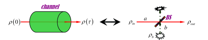
Figure 1: (Colour online) Theoretical equivalent model. Optical fields propagation in realistic environment, can be equivalent to the optical field propagation in a optical channel formalism and also can be abstracted to a fictitious beam-splitter formalism .The correspondences include $\rho\left(0\right)\Longleftrightarrow\rho_{in}$; $\rho\left(\tau\right)\Longleftrightarrow\rho_{out}$.

Our equivalent model ia shown in Fig.1. There exist the one-to-one correspondence between the optical-channel formalism and the BS formalism. In their respective formalism, we have

$$\left(\begin{array}[]{c}a\left(\tau\right)\\ b\left(\tau\right)\end{array}\right)=\left(\begin{array}[]{cc}e^{-\kappa\tau/2}&\sqrt{1-e^{-\kappa\tau}}\\ -\sqrt{1-e^{-\kappa\tau}}&e^{-\kappa\tau/2}\end{array}\right)\left(\begin{array}[]{c}a\left(0\right)\\ b\left(0\right)\end{array}\right)\Longleftrightarrow B\left(\begin{array}[]{c}a\\ b\end{array}\right)B^{{\dagger}}=\left(\begin{array}[]{cc}t&r\\ -r&t\end{array}\right)\left(\begin{array}[]{c}a\\ b\end{array}\right).$$ (2)

In optical-channel formalism, $a\left(\tau\right)$ is the attenuated light mode, $b\left(\tau\right)$ is a flunctutation mode, and $\kappa$ is a damping constant. While in the BS formalism, we defined the BS operator $B=\exp\left(\theta\left(a^{{\dagger}}b-ab^{{\dagger}}\right)\right)$ in terms of the creation (annihilation) operator $a^{{\dagger}}$ ($a$) and $b^{{\dagger}}$ ($b$) with the transmission coefficient $t=\cos\theta$ and $r=\sin\theta$. The relationship can be linked by $t=e^{-\kappa\tau/2}$, $r=\sqrt{\left(1-e^{-\kappa\tau}\right)}$, and $\rho\left(0\right)\Longleftrightarrow\rho_{in}$; $\rho\left(\tau\right)\Longleftrightarrow\rho_{out}$. It should be emphased that $t$ is the transmission coefficient of the BS and $\tau$ is the time of the optical field propagation in the channel.

As pointed in Ref.9 , the simple intuitive model is exact for dissipation in Gaussian reservoirs. Hence, we take a squeezed thermal state (a general Gaussian quantum state), i.e.

$$\rho_{b}=S\left(\lambda\right)\rho_{th}\left(\bar{n}\right)S^{{\dagger}}\left(\lambda\right),$$ (3)

as the environment. This environment can be reduced the reservoirs of vacuum ($\bar{n}=\lambda=0$), thermal ($\lambda=0$), or squeezed vacuum ($\bar{n}=0$). By the way, $S\left(\lambda\right)=\exp\left[\frac{\lambda}{2}\left(a^{\dagger 2}-a^{2}\right)\right]$ is the single-mode squeezed operator with real squeezing parameter $r$. Moreover, $\rho_{{}_{th}}\left(\bar{n}\right)=\sum_{n=0}^{\infty}\frac{\bar{n}^{n}}{\left(\bar{n}+1\right)^{n+1}}\left|n\right\rangle\left\langle n\right|$ is a thermal state with the average photon number $\bar{n}$.

III Beam splitter formalism

In this section, we shall derive the output density operator, the output photon number distribution, and the output WF in the BS formalism.

III.1 Density operator

By using the Weyl expansion of the density operator 10 ; 11 , we can express $\rho_{in}$ and $\rho_{b}$ in the CF formalism

$$\rho_{in}=\int\frac{d^{2}\alpha}{\pi}\chi_{in}\left(\alpha\right)D_{a}\left(-\alpha\right),$$ (4)

and

$$\rho_{b}=\int\frac{d^{2}\beta}{\pi}\chi_{b}\left(\beta\right)D_{b}\left(-\beta\right)$$ (5)

where $D_{a}\left(\alpha\right)=\exp\left(\alpha a^{{\dagger}}-\alpha^{\ast}a\right)$ is the displacement operator in mode $a$, and $\chi_{in}\left(\alpha\right)=$Tr$\left(\rho_{in}D_{a}\left(\alpha\right)\right)$ is the CF of $\rho_{in}$. Similarly, $D_{b}\left(\beta\right)=\exp\left(\beta b^{{\dagger}}-\beta^{\ast}b\right)$ is the displacement operator in mode $b$, and $\chi_{b}\left(\beta\right)=$Tr$\left(\rho_{b}D_{b}\left(\beta\right)\right)=\exp\left(-M\left|\beta\right|^{2}+N\beta^{2}+N\beta^{\ast}{}^{2}\right)$ is the CF of $\rho_{b}$ with $M=\left(\bar{n}+\frac{1}{2}\right)\allowbreak\cosh 2\lambda$ and $N=\allowbreak\frac{1}{2}\left(\bar{n}+\frac{1}{2}\right)\sinh 2\lambda$.

Substituting Eqs. (4) and (5) into Eq.(1) and using the BS transformation relations, we have

$$\rho_{out} = \int\frac{d^{2}\alpha}{\pi}\int\frac{d^{2}\beta}{\pi}\chi_{in}\left(\alpha\right)\chi_{b}\left(\beta\right)D_{a}\left(\left(r\beta-t\alpha\right)\right)\mathrm{Tr}_{b}\left[D_{b}\left(-\left(r\alpha+t\allowbreak\beta\right)\right)\right]$$ (6)

$$= \frac{1}{t^{2}}\int\frac{d^{2}\alpha}{\pi}\chi_{in}\left(\alpha\right)D_{a}\left(-\frac{1}{t}\alpha\right)\exp\left(-X\left|\alpha\right|^{2}+Y\alpha^{2}+Y\alpha^{\ast 2}\right).$$

with $X=Mr^{2}/t^{2}$ and $Y=Nr^{2}/t^{2}$. In the above step, we have used the relation $\mathrm{Tr}_{b}\left[D_{b}\left(-\left(r\alpha+t\allowbreak\beta\right)\right)\right]=\pi\delta^{(2)}\left(-\left(r\alpha+t\allowbreak\beta\right)\right)$ and $\delta^{(2)}\left(-\left(r\alpha+t\allowbreak\beta\right)\right)=\frac{1}{t^{2}}\delta^{(2)}\left(-\left(\frac{r}{t}\alpha+\beta\right)\right)$ 12 . Eq.(6) can also be written as

$$\rho_{out}=\int\frac{d^{2}\alpha}{\pi}\chi_{in}\left(t\alpha\right)D_{a}\left(-\alpha\right)\exp\left(-Mr^{2}\left|\alpha\right|^{2}+Nr^{2}\alpha^{2}+Nr^{2}\alpha^{\ast 2}\right).$$ (7)

Therefore, once the input CF $\chi_{in}\left(\alpha\right)$ is known, then the density operator of the output optical field can be obtained by performing the integration in Eqs. (6) or (7).

III.2 Photon number distribution

The PND is a key characteristic of every optical field. All interesting states of the field are constructed as a combination of Fock states, and different combinations have different quantum properties. Optical field propagation at different time has different character by analyzing the PND. Noticing the definition of the PND, i.e. $P_{out}\left(n\right)=\left\langle n\right|\rho_{out}\left|n\right\rangle$ and using Eq.(7), we have

$$P_{out}\left(n\right) = \frac{1}{n!}\frac{d^{2n}}{dh^{n}ds^{n}}\int\frac{d^{2}\alpha}{\pi}\chi_{in}\left(\alpha t\right)\exp\left(-\left(Mr^{2}+\frac{1}{2}\right)\left|\alpha\right|^{2}\right)$$ (8)

$$\times\exp\left(+Nr^{2}\alpha^{2}+Nr^{2}\alpha^{\ast 2}+\allowbreak h\alpha^{\ast}-s\alpha+hs\right)|_{s=h=0}$$

where we have used that $D_{a}\left(-\alpha\right)=e^{\frac{\left|\alpha\right|^{2}}{2}}e^{\alpha^{\ast}a}e^{-\alpha a^{{\dagger}}}$ and $\left\langle n\right|=\left\langle 0\right|\frac{1}{\sqrt{n!}}\frac{d^{n}}{ds^{n}}\exp\left(sa\right)|_{s=0}$ as well as $\left|n\right\rangle\frac{1}{\sqrt{n!}}\frac{d^{n}}{dh^{n}}\exp\left(ha^{{\dagger}}\right)|_{h=0}\left|0\right\rangle$. Here, we remain the differential form. Thus, once the input CF is known, then the output PND can be obtained by performing the integration in Eq. (8).

III.3 Wigner function

The WF is a well-known quantum mechanical quasi-distribution function used extensively in molecular and quantum optical computations as well as in various theoretical contexts 13 , whose negativity is a witness of the nonclassicality of a quantum state 14 . For a single-mode density operator $\rho$, the WF in the coherent state representation $\left|z\right\rangle$ can be expressed as

$$W(\varepsilon)=\frac{2e^{2\left|\varepsilon\right|^{2}}}{\pi}\int\frac{d^{2}z}{\pi}\left\langle-z\right|\rho\left|z\right\rangle\exp\left(2\varepsilon z^{\ast}-2z\varepsilon^{\ast}\right),$$ (9)

with $\varepsilon=\left(x+ip\right)/\sqrt{2}$. Thus, we have the WF

$$W_{in}(\varepsilon)=\frac{1}{\pi}\int\frac{d^{2}\alpha}{\pi}\chi_{in}\left(\alpha\right)\exp\left(-\alpha\varepsilon^{\ast}+\varepsilon\alpha^{\ast}\right),$$ (10)

for the input state $\rho_{in}$ and

$$W_{out}(\varepsilon) = \frac{1}{\pi}\frac{1}{t^{2}}\int\frac{d^{2}\alpha}{\pi}\chi_{in}\left(\alpha\right)\exp\left(-\frac{1}{t}\alpha\allowbreak\varepsilon^{\ast}+\frac{1}{t}\varepsilon\alpha^{\ast}\right)$$ (11)

$$\times\exp\left(-X\alpha\alpha^{\ast}+Y\alpha^{2}+Y\alpha^{\ast}{}^{2}\right),$$

for the output state $\rho_{out}$. Next, we try our best to find the input-output relationship of the WF.

Recalling the following identity 15 ; 16

$$\int\frac{d^{2}z}{\pi}\exp\left(\zeta\left|z\right|^{2}+\xi z+\eta z^{\ast}+fz^{2}+gz^{\ast 2}\right)$$

$$=\frac{1}{\sqrt{\zeta^{2}-4fg}}\exp\left(\frac{1}{\zeta^{2}-4fg}\left(-\zeta\xi\eta+\xi^{2}g+\eta^{2}f\right)\right),$$ (12)

we find

$$\exp\left(-X\alpha\alpha^{\ast}+Y\alpha^{2}+Y\alpha^{\ast}{}^{2}\right)$$ (13)

$$= \sqrt{\frac{1}{X^{2}-4Y^{2}}}\int\frac{d^{2}\gamma}{\pi}\exp\left(-\frac{X}{X^{2}-4Y^{2}}\left|\gamma\right|^{2}\right)$$

$$\times\exp\left(+i\alpha^{\ast}\gamma+i\alpha\gamma^{\ast}-\frac{Y}{X^{2}-4Y^{2}}\gamma^{2}-\frac{Y}{X^{2}-4Y^{2}}\gamma^{\ast 2}\right).$$

Then we change Eq.(13) into

$$W_{out}(\varepsilon) = \sqrt{\frac{1}{X^{2}-4Y^{2}}}\frac{1}{t^{2}}\int\frac{d^{2}\gamma}{\pi}W_{in}(\frac{1}{t}\varepsilon+i\gamma)$$ (14)

$$\times\exp\left(-\frac{X}{X^{2}-4Y^{2}}\left|\gamma\right|^{2}-\frac{Y}{X^{2}-4Y^{2}}\gamma^{2}-\frac{Y}{X^{2}-4Y^{2}}\gamma^{\ast 2}\right),$$

that is,

$$W_{out}(\varepsilon) = \frac{\allowbreak 2}{T}\int\frac{d^{2}\gamma}{\pi}W_{in}(\frac{1}{t}\varepsilon+i\gamma)$$ (15)

$$\times\exp\left(-\frac{2t^{2}\cosh 2\lambda}{T}\left|\gamma\right|^{2}-\frac{t^{2}\sinh 2\lambda}{T}\gamma^{2}-\frac{t^{2}\sinh 2\lambda}{T}\gamma^{\ast 2}\right),$$

with $T=r^{2}\left(2\bar{n}+1\right)$.

Replacing $z=\frac{1}{t}\varepsilon+i\gamma$, then we change Eq.(15) in another form as follows

$$W_{out}(\varepsilon) = \allowbreak\frac{2}{T}\int\frac{d^{2}z}{\pi}W_{in}(z)\exp\left(-\frac{2\cosh 2\lambda}{T}\left|zt-\varepsilon\right|^{2}\right)$$ (16)

$$\times\exp\left(\frac{\sinh 2\lambda}{T}\left(zt-\varepsilon\right)^{2}+\frac{\sinh 2\lambda}{T}\left(z^{\ast}t-\varepsilon^{\ast}\right)^{2}\right).$$

Thus the transformation formula of the input-output WF in the BS formalism have been obtained. Once the input WF is known, then the output WF can be obtained by performing the integration in Eq. (15) or (16).

IV Optical-channel formalism

Now, we come back to the realistic situation. Noticing the correspondences between the BS formalism and the optical-channel formalism, i.e., $t=e^{-\kappa\tau/2},r=\sqrt{\left(1-e^{-\kappa\tau}\right)}$, we can easily obtain the time evolution formulas of the density operator, the PND and the WF at the moment $\tau$ from Eqs.(7), (8) and (16).

IV.1 Density operator

From Eq.(7), we obtain the density operator of the optical field at any time

$$\rho\left(\tau\right) = \int\frac{d^{2}\alpha}{\pi}\chi\left(\alpha e^{-\kappa\tau/2};0\right)D_{a}\left(-\alpha\right)\exp\left(-M\left(1-e^{-\kappa\tau}\right)\left|\alpha\right|^{2}\right)$$ (17)

$$\times\exp\left(N\left(1-e^{-\kappa\tau}\right)\alpha^{2}+N\left(1-e^{-\kappa\tau}\right)\alpha^{\ast 2}\right).$$

where $\chi\left(\alpha;0\right)$ is the CF of the initial state $\rho\left(0\right)$. Hence, as long as we know the initial CF, we can obtain the density operator at any time.

IV.2 Photon number distribution

From Eq.(8), we obtain the PND of the optical field at any time

$$P\left(n;\tau\right) = \frac{1}{n!}\frac{d^{2n}}{dh^{n}ds^{n}}\int\frac{d^{2}\alpha}{\pi}\chi\left(\alpha e^{-\kappa\tau/2};0\right)\exp\left(-\left(M\left(1-e^{-\kappa\tau}\right)+\frac{1}{2}\right)\left|\alpha\right|^{2}\right)$$ (18)

$$\times\exp\left(N\left(1-e^{-\kappa\tau}\right)\alpha^{2}+N\left(1-e^{-\kappa\tau}\right)\alpha^{\ast 2}+\allowbreak h\alpha^{\ast}-s\alpha+hs\right)|_{s=h=0}.$$

One can verify the correctness of this formula in two extreme cases, i.e. $\tau\rightarrow 0$ and $\tau\rightarrow\infty$. Once the initial CF is known, then the final PND can be obtained by performing the integration in Eq. (18).

IV.3 Wigner function

Using the correspondences $W_{in}(z)\rightarrow W(z;0)$ and $W_{out}(z)\rightarrow W(\varepsilon;\tau)$, Eq.(16) can further expressed as

$$W(\varepsilon;\tau) = \allowbreak\frac{2}{T}\int\frac{d^{2}z}{\pi}W(z;0)\exp\left(-\frac{2\cosh 2\lambda}{T}\left|ze^{-\kappa\tau/2}-\varepsilon\right|^{2}\right)$$ (19)

$$\times\exp\left(\frac{\sinh 2\lambda}{T}\left(ze^{-\kappa\tau/2}-\varepsilon\right)^{2}+\frac{\sinh 2\lambda}{T}\left(z^{\ast}e^{-\kappa\tau/2}-\varepsilon^{\ast}\right)^{2}\right),$$

with $T=\left(2\bar{n}+1\right)\left(1-e^{-\kappa\tau}\right)$. This is an important result, which shows the evolution formula of the WF for the optical field through the optical channel. Thus once the initial WF is known, the WF at any time can be obtained by performing the integration in Eq. (19). In particular, when $\lambda=0$, $\bar{n}=0$, Eq.(19) is reduced to the result in Ref.17 . Moreover, when $\kappa\tau\rightarrow\infty$, $W(\varepsilon;\tau)\rightarrow W_{\rho_{b}}(\varepsilon)$, just like in Appendix A.

V Application of the evolution formulas

Actually, we have derive some general formulas in the general Gaussian reservoir (or environment) with squeezed thermal state. However, for the sake of simplicity, we discuss the time evolution of the PND and the WF by taking thermal channel (that is, we set $\lambda=0$ and $M=\bar{n}+\frac{1}{2},N=0$) and the initial single-photon-added coherent state

$$\left|\psi_{a}\right\rangle=\frac{1}{\sqrt{\Gamma}}a^{{\dagger}}\left|\varkappa\right\rangle.$$ (20)

Here $\left|\varkappa\right\rangle$ is a coherent state and $\Gamma=1+\left|\varkappa\right|^{2}$ is the normalization factor.

V.1 Photon number distribution

Using Eq.(30) and (18), we have

$$P\left(n;\tau\right) = \frac{\Lambda}{n!\Gamma}\frac{d^{2+2n}}{dh_{1}ds_{1}dh^{n}ds^{n}}\exp\left(+\allowbreak\varkappa h_{1}+\allowbreak s_{1}\varkappa^{\ast}+h_{1}s_{1}+hs\right)$$ (21)

$$\times\exp\left(\Lambda\left(\allowbreak h_{1}e^{-\kappa\tau/2}+\varkappa^{\ast}e^{-\kappa\tau/2}-s\right)\left(h-\varkappa e^{-\kappa\tau/2}-s_{1}\allowbreak e^{-\kappa\tau/2}\right)\right)|_{s=h=s_{1}=h_{1}=0},$$

with $\Lambda=\left(\allowbreak\bar{n}-\bar{n}e^{-\kappa\tau}+1\right)^{-1}$. After verification, we find that $P\left(n;0\right)\rightarrow P_{\left|\psi_{a}\right\rangle}\left(n\right)$ and $P\left(n;\infty\right)\rightarrow\bar{n}^{n}/\left(\bar{n}+1\right)^{n+1}$ as expected.

In Fig.2, we plot the PND for two different cases with (a) $\varkappa=0.5+0.5i$ $\bar{n}=0.5$ and (b) $\varkappa=1$, $\bar{n}=0.3$ at different evolution time. The blue, purple, brown and green bars are corresponding to the cases at $\kappa\tau=0$, $\kappa\tau=0.05$, $\kappa\tau=0.25$, and $\kappa\tau\rightarrow\infty$. Taking $P\left(0\right)$ as an example, as shown for the first bars in Fig.2 (a), the zero-photon component $P\left(0\right)$ is increasing with the evolution time $\kappa\tau$, where we find $P\left(0\right)=$0 at $\kappa\tau=0$, $P\left(0\right)=$0.0302572 at $\kappa\tau=0.05$, $P\left(0\right)=$0.145164 at $\kappa\tau=0.25$, and $P\left(0\right)=$0.666667 at $\kappa\tau\rightarrow\infty$.

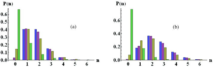
Figure 2: (Colour online) Time evolution of the photon number distribution for a single-photon-addition coherent state as the initial state through thermal channel with (a) $\varkappa=0.5+0.5i$ $\bar{n}=0.5$; (b) $\varkappa=1$, $\bar{n}=0.3$. The blue, purple, brass and green bars are corresponding to the cases $\kappa\tau=0$, $\kappa\tau=0.05$, $\kappa\tau=0.25$, and $\kappa\tau\rightarrow\infty$ (i.e. the thermal state).

V.2 Wigner function

Substituting Eq.(31) into Eq.(19), we have

$$W(\varepsilon;\tau)=\frac{2}{\pi\Gamma}\left(g_{1}\left|\varkappa\right|^{2}-2g_{2}\varkappa\varepsilon^{\ast}-2g_{2}\varkappa^{\ast}\varepsilon+4g_{3}\left|\varepsilon\right|^{2}-g_{4}\right)\exp\left(-2g\left|\varkappa e^{-\kappa\tau/2}-\varepsilon\right|^{2}\right),$$ (22)

with $g_{1}=\left(2ge^{-\kappa\tau}-1\right)^{2}g$, $g_{2}=\allowbreak 2g^{3}e^{-3\kappa\tau/2}-g^{2}e^{-\kappa\tau/2}$, $g_{3}=g^{3}e^{-\kappa\tau}$, $g_{4}=2g^{2}e^{-\kappa\tau}-g$, and $g=\left(2\bar{n}-2\bar{n}e^{-\kappa\tau}+1\right)^{-1}$. In particular, when $\kappa\tau\rightarrow 0$, we find that $W(\varepsilon;0)\rightarrow W_{\left|\psi_{a}\right\rangle}(\varepsilon)$, (see appendix B (3)); while $\kappa\tau\rightarrow\infty$, we have $W(\varepsilon;\infty)=\frac{2}{\pi}\frac{1}{2\bar{n}+1}\exp\left(-\frac{2}{2\bar{n}+1}\left|\varepsilon\right|^{2}\right)$, (see appendix A (3) with $\lambda=0$) which is just the WF of the thermal state, also the environment, as expected.

In Fig.3, we plot the WFs for the case $\varkappa=0.5+0.5i$, $\bar{n}=0.5$ at $\kappa\tau=0$, $\kappa\tau=0.05$, $\kappa\tau=0.25$, and $\kappa\tau\rightarrow\infty$. With the increase of time, the negativity of the WF gradually decreases until it disappears.

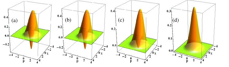
Figure 3: (Colour online) Time evolution of the Wigner function for a single-photon-addition coherent state with $\varkappa=0.5+0.5i$ as the initial state in thermal channel with $\bar{n}=0.5$. (a) $\kappa\tau=0$; (b) $\kappa\tau=0.05$; (c) $\kappa\tau=0.25$; (d) $\kappa\tau\rightarrow\infty$ (i.e. the thermal state).

VI Conclusion

In this paper, we have explored the problem on the optical fields propagation in realistic environments. For our purpose, we have abstracted it into the optical-channel formalism and the BS formalism. In the BS formalism, we derive the input-output relation of the density operator in the CF formalism, which is convenient for obtaining the formulas of the PND and the WF. Using the correspondences of these two formalisms, we easily obtain the time evolution formulas of the density operator, the PND and the WF. These formulas are very important in quantum optics and quantum statistics. As long as we know the CF or the WF of the initial optical field, we can readily find the statistical properties of the optical fields at any time. As an example, we have discussed the case of the single-photon-added coherent state propagated in thermal channel.

Appendix A: Some character of squeezed thermal state

In this appendix, we give a good expression of the density operator and then calculate the CF and WF for squeezed thermal state.

1) Density operator

Recalling the P-function of squeezed thermal state $\rho_{b}$

$$\rho_{b}=\frac{1}{\bar{n}}\int\frac{d^{2}\eta}{\pi}e^{-\frac{1}{\bar{n}}\left|\eta\right|^{2}}S\left(\lambda\right)\left|\eta\right\rangle\left\langle\eta\right|S^{{\dagger}}\left(\lambda\right).$$ (23)

and noticing the squeezing operator $S\left(\lambda\right)=\int\frac{dx}{\sqrt{e^{-\lambda}}}\left|\frac{x}{e^{-\lambda}}\right\rangle\left\langle x\right|$ with $\left|x\right\rangle=\pi^{-\frac{1}{4}}e^{-x^{2}/2+\sqrt{2}xb^{{\dagger}}-b^{{\dagger}2}/2}\left|0\right\rangle$, leading to

$$S\left(\lambda\right)\left|\eta\right\rangle=\frac{1}{\sqrt{\mu}}\exp\left(-\frac{\left|\eta\right|^{2}}{2}-\frac{\nu}{2}\eta^{2}+\frac{\eta}{\mu}b^{{\dagger}}+\frac{\nu}{2}b^{{\dagger}2}\right)\left|0\right\rangle,$$ (24)

with $\mu=\cosh\lambda$ and $\nu=\tanh\lambda$, we know

$$\rho_{b} = \frac{1}{\mu\bar{n}}\int\frac{d^{2}\eta}{\pi}\exp\left(-\frac{1}{\bar{n}}\left|\eta\right|^{2}-\left|\eta\right|^{2}-\frac{\nu}{2}\eta^{2}-\frac{\nu}{2}\eta^{\ast 2}\right)$$ (25)

$$\times\exp\left(\frac{1}{\mu}\eta b^{{\dagger}}+\frac{\nu}{2}b^{{\dagger}2}\right)\left|0\right\rangle\left\langle 0\right|\exp\left(\frac{1}{\mu}\eta^{\ast}b+\frac{\nu}{2}b^{2}\right).$$

This expression of the density operator can help us calculate its statistical properties.

2) Characteristic function

The CF of squeezed thermal state is given by $\chi_{b}\left(\beta\right)=$Tr$\left(\rho_{b}D_{b}\left(\beta\right)\right)$ with $D_{b}\left(\beta\right)=e^{\left|\beta\right|^{2}/2}e^{-\beta^{\ast}b}e^{\beta b^{{\dagger}}}$ 18 . Thus, we have

$$\chi_{b}\left(\beta\right) = \frac{1}{\mu\bar{n}}e^{\frac{\left|\beta\right|^{2}}{2}}\int\frac{d^{2}\eta}{\pi}\exp\left(-\frac{1}{\bar{n}}\left|\eta\right|^{2}-\left|\eta\right|^{2}-\frac{\nu}{2}\eta^{2}-\frac{\nu}{2}\eta^{\ast 2}\right)$$ (26)

$$\left\langle 0\right|\exp\left(\frac{1}{\mu}\eta^{\ast}b-\beta^{\ast}b+\frac{\nu}{2}b^{2}\right)\exp\left(\frac{1}{\mu}\eta b^{{\dagger}}+\beta b^{{\dagger}}+\frac{\nu}{2}b^{{\dagger}2}\right)\left|0\right\rangle$$

$$= \exp\left(-M\left|\beta\right|^{2}+N\beta^{2}+N\beta^{\ast}{}^{2}\right).$$

3) Wigner function

Using Eqs.(9) and (25), we obtain the WF of the squeezed thermal state as follows

$$W_{\rho_{b}}(\varepsilon)=\frac{2}{\pi}\frac{1}{2\bar{n}+1}\exp\left(-2\frac{\cosh 2\lambda}{2\bar{n}+1}\left|\varepsilon\right|^{2}+\frac{\sinh 2\lambda}{2\bar{n}+1}\varepsilon^{2}+\allowbreak\frac{\sinh 2\lambda}{2\bar{n}+1}(\varepsilon^{\ast})^{2}\right).$$ (27)

Appendix B: Some character of single-photon-added coherent state

In this appendix, we derive the normalization factor, the CF and the WF for the single-photon-added coherent state $\left|\psi_{a}\right\rangle=\frac{1}{\sqrt{\Gamma}}a^{{\dagger}}\left|\varkappa\right\rangle$. The density operator $\rho_{a}=\left|\psi_{a}\right\rangle\left\langle\psi_{a}\right|$ can be expressed as

$$\rho_{a}=\frac{1}{\Gamma}\exp\left(-\left|\varkappa\right|^{2}\right)\frac{d^{2}}{dh_{1}ds_{1}}\exp\left(s_{1}a^{{\dagger}}+\varkappa a^{{\dagger}}\right)\left|0\right\rangle\left\langle 0\right|\exp\left(h_{1}a+\varkappa^{\ast}a\right)|_{s_{1}=h_{1}=0},$$ (28)

1) Normalization factor

Using Tr$\left(\rho_{a}\right)=1$, we have the normalization factor

$$\Gamma = \exp\left(-\left|\varkappa\right|^{2}\right)\left\langle 0\right|\exp\left(h_{1}a+\varkappa^{\ast}a\right)\exp\left(s_{1}a^{{\dagger}}+\varkappa a^{{\dagger}}\right)\left|0\right\rangle|_{s_{1}=h_{1}=0}$$ (29)

$$= \exp\left(-\left|\varkappa\right|^{2}\right)\frac{d^{2}}{dh_{1}ds_{1}}\exp\left(\left(h_{1}+\varkappa^{\ast}\right)\left(s_{1}+\varkappa\right)\right)|_{s_{1}=h_{1}=0}$$

$$= 1+\left|\varkappa\right|^{2},$$

2) characteristic function

Substituting $D_{a}\left(\alpha\right)=e^{\frac{\left|\alpha\right|^{2}}{2}}e^{-\alpha^{\ast}a}e^{\alpha a^{{\dagger}}}$ and Eq.(28) into $\chi_{in}\left(\alpha\right)=$Tr$\left(\rho_{a}D_{a}\left(\alpha\right)\right)$, we obtain the CF as follows

$$\chi_{in}\left(\alpha\right) = \frac{1}{\Gamma}\exp\left(\frac{\left|\alpha\right|^{2}}{2}-\left|\varkappa\right|^{2}\right)\frac{d^{2}}{dh_{1}ds_{1}}\exp\left(\left(h_{1}+\varkappa^{\ast}-\alpha^{\ast}\right)\left(s_{1}+\varkappa+\alpha\right)\right)|_{s_{1}=h_{1}=0}$$ (30)

$$= \frac{1}{\Gamma}\left(\alpha\varkappa^{\ast}-\left|\alpha\right|^{2}-\varkappa\alpha^{\ast}+\left|\varkappa\right|^{2}+1\right)\exp\left(-\frac{\left|\alpha\right|^{2}}{2}+\alpha\varkappa^{\ast}-\varkappa\alpha^{\ast}\right)\allowbreak$$

3) Wigner function

Substituting Eq.(28) into Eq.(9), we obtain the WF

$$W_{\left|\psi_{a}\right\rangle}(\varepsilon) = \frac{2}{\pi\Gamma}\exp\left(2\left|\varepsilon\right|^{2}-\left|\varkappa\right|^{2}\right)\frac{d^{2}}{dh_{1}ds_{1}}\exp\left(\left(h_{1}+\varkappa^{\ast}-2\varepsilon^{\ast}\right)\left(2\varepsilon-s_{1}-\varkappa\right)\right)|_{s_{1}=h_{1}=0}$$ (31)

$$= \frac{2}{\pi\Gamma}\left(\varkappa\varkappa^{\ast}-2\varkappa\varepsilon^{\ast}-2\varepsilon\varkappa^{\ast}+\allowbreak 4\varepsilon\varepsilon^{\ast}-1\right)\exp\left(-2\left|\varkappa-\varepsilon\right|^{2}\right).$$

References

- (1) M. O. Scully and M. S. Zubairy, Quantum optics (Cambridge University Press, 1997).
- (2) H. J. Carmichael, Statistical methods in quantum Optics 1 (Springer-Verlag Berlin Heidelberg, 1999).
- (3) H. J. Carmichael, An open systems approach to quantum optics (Springer-Verlag Berlin Heidelberg, 1999).
- (4) U. Weiss, Quantum Dissipative Systems (World Scientific, Singapore, 1999).
- (5) B. Daeubler, H. Risken, and L. Schoendorff, Phys. Rev. A 48, 3955 (1993).
- (6) H. J. Briegel and B. G. Englert, Phys. Rev. A 47, 3311 (1993).
- (7) G. M. d’Ariano, Phys. Lett. A 187, 231 (1994).
- (8) H. Y. Fan and L. Y. Hu, Mod. Phys. lett. B 22, 2435 (2008).
- (9) U. Leonhardt, Phys. Rev. A 48, 3265 (1993).
- (10) G. D. Palma, A. Mari, V. Giovannetti, and A. S. Holevo, J. Math. Phys. 56, 052202 (2015).
- (11) L. Y. Hu, Z. Y. Liao, S. L. Ma, and M. S. Zubairy, Phys. Rev. A 93, 033807 (2016).
- (12) S. M. Barnett and P. M. Radmore, Methods in theoretical quantum optics (Clarendon Press, Oxford, 1997).
- (13) S. H. H. Chowdhury and S. T. Ali, J. Math. Phys. 56, 122102 (2015).
- (14) A. Kenfack, K. Zyczkowski, J. Opt. B, Quantum Semiclass. Opt. 6, 396 (2004).
- (15) R. R. Puri, Mathematical Methods of Quantum Optics (Springer-Verlag, Berlin, 2001).
- (16) N. Spagnolo, C. Vitelli, T. D. Angelis, F. Sciarrino, and F. D. Martini, Phys. Rev. A 80, 032318 2009.
- (17) L. Y. Hu and H. Y. Fan, Opt. Commun. 282, 4379 (2009).
- (18) F. Parisio, J. Math. Phys. 57, 032101 (2016).